Abstract
The Zika virus model (ZIKV) is mathematically modeled to create the perfect control strategies. The main characteristics of the model without control strategies, in particular reproduction number, are specified. Based on the basic reproduction number, if , then ZIKV satisfies the disease-free equilibrium. If , then ZIKV satisfies the endemic equilibrium. We use the maximum principle from Pontryagin’s. This describes the critical conditions for optimal control of ZIKV. Notwithstanding, due to the prevention and treatment of mosquito populations without spraying, people infected with the disease have decreased dramatically. Be that as it may, there has been no critical decline in mosquitoes contaminated with the disease. The usage of preventive treatments and insecticide procedures to mitigate the spread of the proposed virus showed a more noticeable centrality in the decrease in contaminated people and mosquitoes. The application of preventive measures including treatment and insecticides has emerged as the most ideal way to reduce the spread of ZIKV. Best of all, to decrease the spread of ZIKV is to use avoidance, treatment and bug spraying simultaneously as control methods. Moreover, for the numerical solution of such stochastic models, we apply the spectral technique. The stochastic or random phenomenons are more realistic and make the model more informative with the additive information. Throughout this paper, the additive term is assumed as additive white noise. The Legendre polynomials and applications are implemented to transform the proposed system into a nonlinear algebraic system.
1. Introduction
The signs of the Zika virus (ZIKV) outbreak initially appeared in Africa which occurred in Yap in April [1,2]. At that point, this was followed by another flare-up in French Polynesia for a time duration of six months from October 2013 to April 2014 [3], and happened in other Pacific states as well [4,5]. A few other cases of ZIKV were recorded within the South American nations. In 2015, Columbia and Brazil had the most casualties [6,7,8]. Basically, the transmission of ZIKV is vector-borne; however, in some cases, it may transmit through the process of blood transfusion and sexual or physical contact. The main reason for transmission is Aedes species mosquitoes as well as the vector of the dengue virus [9]. ZIKV has been distinguished as being able to carry transmission in a few tropical climate zones [10]. ZIKV pointers contain fever, ailment, expanded predominance of neurological sequelae and microcephaly within newborn babies to moms who have gotten ZIKV amid pregnancy [11,12]. The latest ZIKV incident in Brazil and French Polynesia may have forced the WHO to declare an International Public Health Emergency Concern in response to microcephaly clusters and other neurological chaos. In addition to the major flare-up of French Polynesia which saw 42 cases of Guillain-Barre disorder between March 2014 and May 2015 within the same locale, 10 cases of Guillain-Barre disorder with microcephaly and extreme brain injuries [11,13] were reported. ZIKV has the potential to spread on a global level; hence, it is critical to illustrate the potential for transmission of the ailment. Mathematical models may offer assistance to direct a limit called reproduction number. The reproduction number is supposed to be capable of predicting the measurement of how the infection will spread [14,15,16]. Moreover, mathematical models can offer assistance to decide the constraint called the birth number which, as a rule, offers data on how the disease will be kept up. Utilizing the application of mathematical models, numerous analysts have examined mosquito-related maladies [17,18,19]. The mathematical model can significantly improve the potential variables for spreading ZIKV. Valuable hypothetical data and ideal time control on both anticipation and treatment of this illness could be key for the World Health Organization to control this illness. An ideal control procedure has been utilized to consider numerous mosquito-related infections. To study several mosquito-related ailments, optimal time control has been utilized. Moreover, the author [20] discusses the genetic diversity in the SIR model of pathogen evolution. Moreover, Lazebnik et al. in [21] used the generic approach for the mathematical model of a multi-strain pandemic and the author [22]’s pandemic management by a spatio-temporal mathematical model.
The mathematical simulation of the proposed pandemic disease is essential because the investigation of the basic reproduction number for different parameter values gives different equilibrium behaviors. As to the best of the researcher’s knowledge, there are no stochastic phenomena models on ZIKV. In this research study, we have come up with a new model with stochastic or random effect to assess the impact of mass treatment and pesticides. The ZIKV disease is one of the most dangerous diseases in human history. Therefore, we discuss the different behaviors of ZIKV disease for the different parameter values. The system was simulated under the human classes along with vector classes because the proposed virus enters the human body through the vector body. The reason for this is to take the random information of Zika-infected agents and vectors at the total of most individuals and pesticides utilizing the progressed Pontryagin regimen.
The stochastic models were used by many authors in the literature: The single time-delayed stochastic integral equations via orthogonal functions are implemented by Seyyedeh N. Kiaee et al. [23]. The minimum superstability of stochastic ternary anti-derivations in symmetric matrix-valued are used by [24]. Similarly, the stochastic analysis of train running safety on a bridge with earthquake-induced irregularity under aftershock was studied by the author [25] and the stochastic SIRS epidemic model using the spectral technique by [26].
2. Model Formulation
The overall population may be divided among five different classes; class of susceptible, class of infected ones, treatment class, infected and susceptible classes in vector population for mathematical modeling. The new birth rate was put in place in vulnerable communities and customary passing proportion . The disposed population gets contaminated with a critical form of hepatitis C and moves to the exposed class E class at the rate of epidemic . Persons in the E class who pass from disease or injury from class E of hepatitis C and move to class with pestilence rate , and those persons recover at a rate and move to the recovered population class S. The individuals in class A, in addition to the usual disease rate , stands for the disease death rate. The persons in class C are cured at amount and switch to susceptible population class S. Those persons constituting compartment C are protected and stimulated to population Q at a rate . The population in Q inflates to the regular disease rate . Moreover, deaths at a disease-induced death rate are indicated by . Persons who are insulated and cured at a rate of b or develop greatly penetrate with HCV at a rate of .
All the notations for parameters and variables in the model Equation (1) are described here.
: Overall amount of the human population.
: The overall community of susceptible individuals.
: Overall infected individuals in the human population.
: Class of treatment in the population.
: Denotes vector population total size.
: Vector susceptible population.
: Vector infected population.
: Recruitment rate of human population.
: Recruitment rate of vector population.
: Rate of effective contact among the infected vector and susceptible humans class.
: Represents the rate of transmission rate from humans (infected) to susceptible vector.
: Contact rate ratio between susceptible and infected humans.
: Human compartment mortality rate.
: Vector compartment mortality rate.
w: Infected humans treatment rate.
: Disease-induced mortality rate.
Applying LaSalle’s invariance principle, we can make a threshold dynamic of Equation (1) using basic Reproduction number . For less than 1 results that Equation (1) has free infection disease equilibrium = (, , , , ) = ( and would be stable asymptotically. Nevertheless, for greater than 1 decide endemic equilibrium = (, , , , ) of the given system to be asymptotically stable.
Stochastic perturbation are assumed to be white noise, and Equation (1) will be deduced to the following form
represents Brownian motion and is also known as the intensity of Brownian motion. The focus of the current study is to accomplish the current method for approximate solution of stochastic SITSI model prescribed in Equation (2). Formerly this method was exhibited by D Lehotzky. He uses this technique for periodic time delay differential equations and stability analysis of such types of equations with distributed and multiple delays. Moreover, N khaji and P Zakian consider in their work the spectral stochastic finite element method for analysis of wave propagation assuming medium uncertainties. Many researchers have used Legender polynomial to approximate solutions of differential and integral equation.
The rest of the article is structured as follows: Section 3 consists of a description of LSCM along with a brief review of Legendre polynomials are given. Section 4 consists of the asymptotic stability of infection-free and endemic equilibrium. Numerical test problems are given in Section 5. In the last Section 6, conclusions are drawn and references are given at the end of this article.
3. Method Description
Before applying the Legendre spectral collocation method, we will provide an overview of Legendre polynomials, refer to [27,28]. , signifies the Legendre polynomials nth order. The function given on the interval is approximated by
indicates Legendre coefficients which are unknowns, signifies interpolating points fulfilling and denotes the nth order. The Legendre polynomial is as follows:
The stochastic model equation SITSI is given by Equation (2). In this section, we have to establish the LSCM to find the solution of the said model equation. LSCM procedure involves Legendre–Guass quadrature points along with weight function. For the current method, Legendre–Gauss–Lobatto points are considered; hence, the roots of . Where defines the th Legendre polynomial.
The aim of this study is to acquire an approximate solution for the model equation Equation (2). For this purpose let take integral on both sides of Equation (2) from 0 to t. It takes the form
where are initial conditions on the functions and , respectively. We use the linear transformation on the standard interval for the purpose to investigate the Legendre spectral collocation method, then Equation (5) becomes:
Semi-discretized spectral equations of Equation (6) are given below:
The Legendre–Gauss (LG) quadrature together with weight function refer [29,30,31,32,33,34] is given by
Moreover, the Legendre–Gauss quadrature along with stochastic weight function is given by
Using the Legendre polynomial for the approximation of , , and by using Equation (5)
Legendre coefficients of the functions , , , and are denoted by , , , and , respectively. Now make use of the above approximation Equation (9) takes the form given below:
Taking for simplicity. The system given in Equation (9) consists of number of unknowns in which nonlinear algebraic equations. Plugging the initial conditions
Equations (9) and (10) form a system of non-linear algebraic equations with unknowns where The above two systems give the value of these unknowns. Putting the values of these unknowns in Equation (8) we obtain an an approximate solution for the proposed model given in Equation (2).
4. Asymptotical Stability of Endemic Equilibrium and Infection-Free Status
Stability analysis is essential to explore the dynamical system. This section includes a discussion of the stochastic asymptotic stability of equilibrium solutions of the deterministic and stochastic systems which are given in Equation (1) and Equation (2), respectively.
A maximum of two equilibrium solutions of the Zika virus model given in Equation (1) may exist, the steady state solution without population disease namely an infection-free equilibrium and the other one is an endemic equilibrium solution.
The following equation gives the reproduction number using next generation method for the system given by Equation (1)
Theorem 1.
Proof.
Let E represents the endemic equilibrium of the system given by Equation (1), then need to persuade the subsequent system
To solve the system given in Equation (13). We will discuss two cases and .
- (a)
- (b)
- we have used the Maple-13 software for these calculations and find the following endemic equilibrium Nonetheless, in this case, .
□
Lemma 1.
The overall region is positively invariant set for stochastic system given in Equations (1).
Proof.
Since , then by system Equation (1), we obtain:
Therefore, by adopting integrating factor technique to solve Equation (15),
Thus, for the system given in Equation (1), the region is positively invariant.
Using the method from [15], the following lemma can be proved. □
Lemma 2.
The solution of system Equation (2) has following properties for each initial condition :
and similarly almost surely for each class.
Definition 1.
Individuals that are infected in humans and vector population and are termed extinctive for the system Equation (2) if and only if .
Theorem 2.
Proof.
Assume the solution of the stochastic Zika virus system given in Equation (2) be that satisfies the initial values . Further, assume that . According to It formula we got the following form
Integrate the system given in Equation (16) from 0 to t, we have
Now, discussing the following two different cases, if , then
Divide Equation (18) by , then
By taking and using Lemma 2, then Equation (19) converted to
Therefore, if , which shows
Theorem 3.
The contaminate population, therefore and exists in Equation (2), if the reproduction number greater than 1. For proof refers to [35].
5. Numerical Results
This section comprises the numerical test problems. The numerical results are obtained and discussed in the deterministic system (1) as well as the stochastic system (2). The Legendre spectral collocation method is used to find the numerical results for the given models. The results obtained are given in Figure 1, Figure 2, Figure 3, Figure 4, Figure 5, Figure 6, Figure 7, Figure 8, Figure 9 and Figure 10. Maple and Matlab software are used for associated computations on a personal computer.
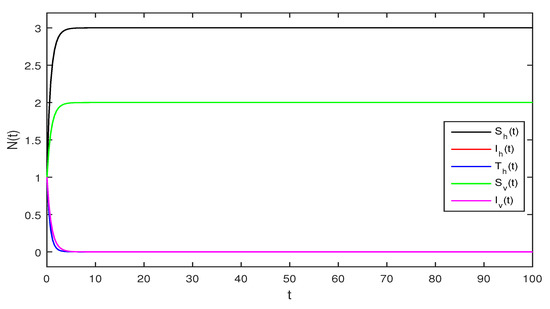
Figure 1.
Deterministic Zika virus system (1) using that is
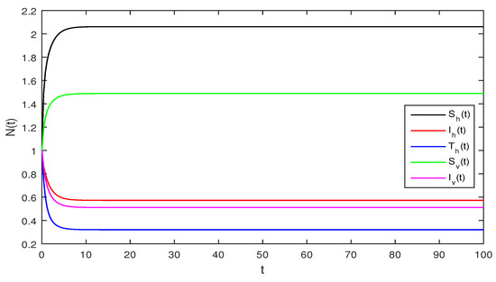
Figure 2.
Deterministic system (1), with that is
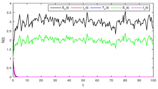
Figure 3.
Solution of stochastic system Equation (2), with where
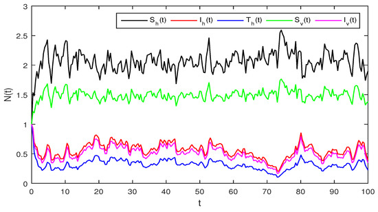
Figure 4.
Solution of stochastic system Equation (2), with where
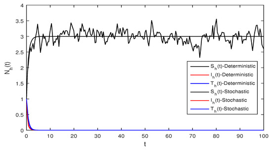
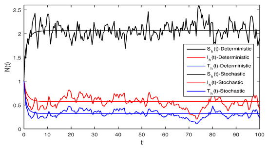
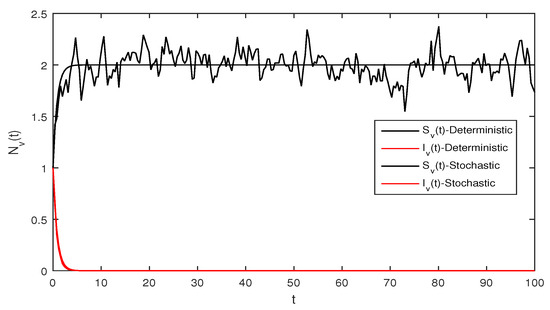
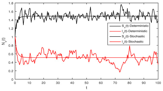
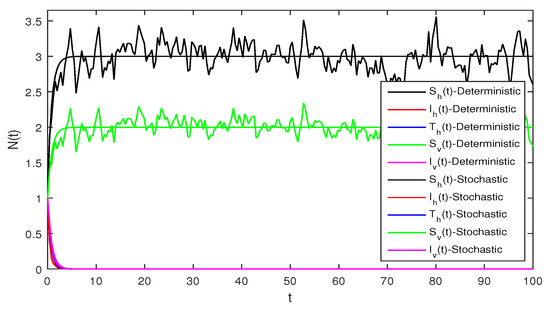
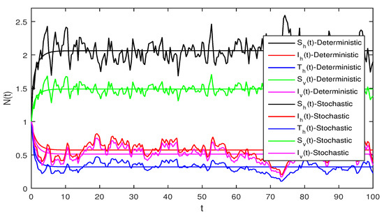
Figure 1 Appropriate parameters values were introduced readily. We assumed for deterministic system Equation (1) the values of parameters as . The computations give reproduction number by using these parameter values. By using Theorem 1 we see that the system given in Equation (1) has stable disease-free equilibrium where the susceptible human individuals are equal to and for the vector population is .
Figure 2 Although, if we take and and assuming the same parameter values as we assumed in Figure 1. The reproduction number is and again using Theorem 1 the system given in Equation (1) has a stable infectious equilibrium and all the classes are non zero which can be seen in Figure 2.
Figure 3 When we chosen parameter values for stochastic system Equation (2). The simple calculation shows the condition and . Using Theorem 2, the infected individuals for both human and vector populations of the system given in Equation (2) approach zero. This behavior can be seen in Figure 3 clearly.
Figure 4 Similarly if we choose and the remaining the same parameter values as in Figure 3, then the simple calculation shows that the deterministic system Equation (2) satisfies the condition , and then by Theorem 2, the infected individuals for human and vector populations are present in a system Equation (2), this can be performed in Figure 4.
Figure 5 This figure shows a comparison for both the stochastic and deterministic systems for humans using the following values of parameters . Using these parameter values, the simple computation shows that for the deterministic system Equation (1) , also for stochastic system Equation (2) , and
Figure 6 Deterministic and stochastic systems for humans are compared in this figure. We chose and the same parameter values as given in Figure 5. Simple computation shows that for the deterministic system Equation (1) and for stochastic system Equation (2) and
6. Conclusions
We solved the suggested model with a stochastic effect successfully using the Legendre spectral method and its characteristics. Moreover, the system has been transformed into a nonlinear equation system by using and deriving the Legendre–Gauss quadrature and Legendre polynomial with weight functions. The research covered both deterministic and stochastic systems. The different behavior of the reproduction are examined for the proposed system. We noticed that when the reproduction number is less than 1, the infected populace approaches 0, which simply implies that the system approaches status (the disease-free equilibrium). Whereas, for reproduction number greater than 0, then the system reached status (unique stable endemic equilibrium). On the other hand, intensities of noise for the stochastic system has been debated for stochastic phenomena. We have observed that the presence of the intensities solution becomes stronger as we shoot up without intensities. Moreover, we compared the solutions of systems given in Equations (1) and (2) for the validation of the proposed method as well. The strategy is comparatively great to solve the stochastic model since the dramatic consequences of ZIKV on public health since 2015 have highlighted the threat that ZIKV represents. Although the pandemic has waned since that time, the virus is still circulating, and areas with competent vectors are at risk of ZIKV re-emergence. An estimated 3.6 billion people live in at-risk areas. Several challenges still need to be addressed such as the development of specific drugs and vaccines, the need for improved epidemiological surveillance in at-risk areas, and the determination of long-term consequences of ZIKV infection, in particular, in cases of prenatal exposure.
In the future, this research work can be extended to the optimal control and fractional derivatives for such types of diseases.
Author Contributions
Methodology, F.U.K. and S.U.K.; validation, E.A.A., W.J. and E.S.M.T.E.D.; formal analysis, S.U.K.; investigation, S.U.K.; data curation, F.U.K.; writing—original draft preparation, F.U.K.; writing—review and editing, E.A.A., S.U.K., W.J. and E.S.M.T.E.D.; visualization, S.U.K.; funding acquisition, E.A.A., W.J. and E.S.M.T.E.D. All authors have read and agreed to the published version of the manuscript.
Funding
This research received no external funding.
Institutional Review Board Statement
Not applicable.
Informed Consent Statement
Not applicable.
Data Availability Statement
Not applicable.
Acknowledgments
The authors acknowledge the financial support provided by University of Tabuk, Saudi Arabia.
Conflicts of Interest
The authors declare no conflict of interest.
References
- Rajasekar, P.S.; Pitchaimani, M. Qualitative analysis of stochastically perturbed SIRS epidemic model with two viruses. J. Chaos Solitons Fractals 2019, 118, 207–221. [Google Scholar] [CrossRef]
- Zhou, Y.; Zhang, W.; Yuan, S.; Hu, H. Persistence and extinction in stochastic SIRS models with general nonlinear incidence rate. Electron. Differ. Eqnarrays 2014, 42, 1–17. [Google Scholar]
- Carletti, M. Mean-square stability of a stochastic model for bacteriophage infection with time delays. Math. Biosci. 2007, 210, 395–414. [Google Scholar] [CrossRef] [PubMed]
- Meng, X.Z.; Chen, L.S. The dynamics of a new SIR epidemic model concerning pulse vaccination strategy. Appl. Math. Comput. 2008, 197, 528–597. [Google Scholar] [CrossRef]
- Lehotzky, D.; Insperger, T.; Stepan, G. Extension of the spectral element method for stability analysis of time-periodic delay-differential equations with multiple and distributed delays. Commun. Nonlinear Sci. Numer. Simul. 2016, 35, 177–189. [Google Scholar] [CrossRef]
- Zakian, P.; Khaji, N. A stochastic spectral finite element method for wave propagation analyses with medium uncertainties. Appl. Math. 2018, 63, 84–108. [Google Scholar] [CrossRef]
- Zhang, F.P.; Li, Z.Z.; Zhang, F. Global stability of an SIR epidemic model with constant infectious period, Appl. Math. Comput. 2008, 199, 285–291. [Google Scholar]
- Pontryagin, L.S.; Boltyanskii, V.G.; Gamkrelidze, R.V.; Mishchenko, E.F.; Trirogoff, K.N. TheMathematical Theory of Optimal Processes; Interscience Publishers: New York, NY, USA, 1962. [Google Scholar]
- Khan, M.A.; Khan, Y.; Khan, T.W.; Islam, S. Dynamical system of a SEIQV epidemic model with nonlinear generalized incidence rate arising in biology. Int. J. Biomath. 2017, 7, 1750096. [Google Scholar] [CrossRef]
- Khan, M.A.; Khan, Y.; Khan, S.; Islam, S. Global stability and vaccination of an SEIVR epidemic model with saturated incidence rate. Int. J. Biomath. 2016, 9, 1650068. [Google Scholar] [CrossRef]
- Roy, M.; Holt, R.D. Effects of predation on hostpathogen dynamics in SIR models. Theor. Popul. Biol. 2008, 73, 319–331. [Google Scholar] [CrossRef]
- Zhang, T.L.; Teng, Z.D. Permanence and extinction for a nonautonomous SIRS epidemic model with time delay. Appl. Math. Model. 2009, 33, 1058–1071. [Google Scholar] [CrossRef]
- Hamer, W.H. Epidemic disease in England. Lancet 1906, 1, 733–739. [Google Scholar]
- Ross, R.A. The Prevention of Malaria; Murray: London, UK, 1911. [Google Scholar]
- Meng, X.; Chen, L.; Wu, B. A delay SIR epidemic model with pulse vaccination and incubation times. Nonlinear Anal. Real World Appl. 2010, 11, 88–98. [Google Scholar] [CrossRef]
- Zhou, J.; Yang, Y.; Zhang, T. Global stability of a discrete multigroup SIR model with nonlinear incidence rate. Math. Methods Appl. Sci. 2017, 40, 5370–5379. [Google Scholar] [CrossRef]
- Zhang, T.; Meng, X.; Zhang, T.; Song, Y. Global dynamics for a new high-dimensional SIR model with distributed delay. Appl. Math. Comput. 2012, 218, 11806–11819. [Google Scholar] [CrossRef]
- Kermack, W.O.; McKendrick, A.G. A contribution to the mathematical theory of epidemics. Proc. R. Soc. Math. Phys. Eng. Sci. 1927, 115, 700–721. [Google Scholar]
- Li, J.; Ma, Z. Qualitative analyses of SIS epidemic model with vaccination and varying total population size. Math. Comput. Model. 2002, 35, 1235–1243. [Google Scholar] [CrossRef]
- Gordo, I.; Gomes, M.G.M.; Reis, D.G.; Campos, P.R.A. Genetic diversity in the SIR model of pathogen evolution. PLoS ONE 2009, 4, e4876. [Google Scholar] [CrossRef]
- Lazebnik, T.; Bunimovich-Mendrazitsky, S. Generic approach for mathematical model of multi-strain pandemics. PLoS ONE 2022, 17, e0260683. [Google Scholar]
- Lazebnik, T.; Bunimovich-Mendrazitsky, S.; Shami, L. Pandemic management by a spatio-temporal mathematical model. Int. J. Nonlinear Sci. Numer. 2021. [Google Scholar] [CrossRef]
- Kiaee, S.N.; Khodabin, M.; Ezzati, R.; Lopes, A.M. A New Approach to Approximate Solutions of Single Time-Delayed Stochastic Integral Equations via Orthogonal Functions. Symmetry 2022, 14, 2085. [Google Scholar] [CrossRef]
- Eidinejad, Z.; Saadati, R.; O’Regan, D.; Alshammari, F.S. Minimum Superstability of Stochastic Ternary Antiderivations in Symmetric Matrix-Valued FB-Algebras and Symmetric Matrix-Valued FC-?-Algebras. Symmetry 2022, 14, 2064. [Google Scholar] [CrossRef]
- Tan, J.; Xiang, P.; Zhao, H.; Yu, J.; Ye, B.; Yang, D. Stochastic Analysis of Train Running Safety on Bridge with Earthquake-Induced Irregularity under Aftershock. Symmetry 2022, 14, 1998. [Google Scholar] [CrossRef]
- Ishtiaq, A.; Khan, S.U. Threshold of Stochastic SIRS Epidemic Model from Infectious to Susceptible Class with Saturated Incidence Rate Using Spectral Method. Symmetry 2022, 14, 1838. [Google Scholar] [CrossRef]
- Gul, N.; Khan, S.U.; Ali, I.; Khan, F.U. Transmission dynamic of stochastic hepatitis C model by spectral collocation method. Comput. Methods Biomech. Biomed. Eng. 2022, 25, 578–592. [Google Scholar] [CrossRef] [PubMed]
- Ali, A.; Khan, S.U.; Ali, I.; Khan, F.U. On dynamics of stochastic avian influenza model with asymptomatic carrier using spectral method. Math. Methods Appl. Sci. 2022, 45, 8230–8246. [Google Scholar] [CrossRef]
- Ullah, K.S.; Ishtiaq, A. Application of Legendre spectral-collocation method to delay differential and stochastic delay differential equation. AIP Adv. 2018, 8, 035301. [Google Scholar]
- Ullah, K.S.; Mushtaq, A.; Ishtiaq, A. A spectral collocation method for stochastic Volterra integro-differential equations and its error analysis. J. Adv. Differ. Equ. 2019, 1, 161. [Google Scholar]
- Ullah, K.S.; Ishtiaq, A. Numerical Analysis of Stochastic SIR Model by Legendre Spectral Collocation Method; Advances in Mechanical Engineering; SAGE Publications Sage: London, UK, 2019; Volume 11, p. 7. [Google Scholar]
- Ishtiaq, A.; Khan, S.U. Analysis of stochastic delayed SIRS model with exponential birth and saturated incidence rate. Chaos Solitons Fractals 2020, 138, 110008. [Google Scholar]
- Ullah, K.S.; Ishtiaq, A. Convergence and error analysis of a spectral collo- cation method for solving system of nonlinear Fredholm integral equations of second kind. Comput. Appl. Math. 2019, 38, 125. [Google Scholar]
- Ullah, K.S.; Ali, I. Applications of Legendre spectral collocation method for solving system of time delay differential equations. Adv.-Mechan-Ical Eng. 2020, 12, 1–13. [Google Scholar]
- Song, Y.; Miao, A.; Zhang, T.; Wang, X.; Liu, J. Extinction and persistence of a stochastic SIRS epidemic model with saturated incidence rate and transfer from infectious to susceptible. Adv. Differ. Equations 2018, 2018, 293. [Google Scholar] [CrossRef]


Publisher’s Note: MDPI stays neutral with regard to jurisdictional claims in published maps and institutional affiliations. |
© 2022 by the authors. Licensee MDPI, Basel, Switzerland. This article is an open access article distributed under the terms and conditions of the Creative Commons Attribution (CC BY) license (https://creativecommons.org/licenses/by/4.0/).