Photoacoustics Waveform Design for Optimal Signal to Noise Ratio

Abstract

Time-frequency analysis in waveform engineering can be applied to many detection and imaging systems, such as radar, sonar, and ultrasound to improve their Signal-to-Noise Ratio (SNR). Recently, photoacoustic imaging systems have attracted researchers’ attention. However, the SNR optimization problem for photoacoustic systems has not been fully addressed. In this paper, the one-dimensional SNR optimization of the photoacoustic response to an input waveform with finite duration and energy was considered. This paper applied an eigenfunction optimization approach to find the waveform for optimal SNR for various photoacoustic absorber profiles. SNR gains via the obtained optimal waveform were compared with simple square-pulse and pulsed sinusoidal waveforms in simulations. Results showed that by using the optimal waveform, SNR can be enhanced especially if the input wave duration is comparable with the absorber time profile duration. The optimal waveforms can achieve 5%–10% higher SNR than square pulses and over 100% higher SNR compared with pulsed sinusoids. The symmetry between time and frequency domains assures similar behavior when temporal durations of the input waveforms are too short or too long compared with the absorber.

1. Introduction

A photoacoustic imaging system for biomedical applications combines the advantages of the optical and acoustical imaging methods. It has the advantages of both sensitive optical absorption contrast [1] and low acoustic scattering in soft tissue [2]. Using safe non-ionizing illumination sources, the photoacoustic effect can be applied to biological tissues. The most common excitation source for photoacoustics has been pulsed electromagnetic waves, for example in the work by Kruger [3,4] and Wang [5,6,7]. In the recent decade, a pulse compression approach via matched filtering was introduced and investigated [8,9,10,11,12,13,14,15]. Different approaches have been studied to improve the SNR of photoacoustic imaging systems, such as using a contrast agent to improve the contrast of the image in photoacoustics application [16], using coherent or incoherent averaging signal processing methods to increase the SNR [13], and optimizing input waveform and receiver-filter to improve SNR [12,17,18,19]. Most recently, Truncated Correlation Photoacoustic Coherence Tomography (TC-PACT) is reported to have higher SNR than pulse compression photoacoustics [20]. The use of the echo effect is also shown to improve SNR more than simple pulsed photoacoustics [21]. Ultrasound-Photoacoustic dual-modality imaging is also used to provide better performance [22]. However, most of the studies are still based on either chirps or square pulses, or occasionally, Gaussian pulses [23] or pulse trains similar to pulsed sinusoids with a high carrier frequency [24]. The detailed methodology behind optimizing the input photoacoustic waveform is still not fully developed in the literature.

In this paper, the SNR optimization for a one-dimensional photoacoustic system and the effect of optimal input waveform selection on SNR were investigated. Additionally, the SNR obtained by the optimal waveform was compared and discussed in relation to commonly used square-pulse and pulsed sinusoid waveforms.

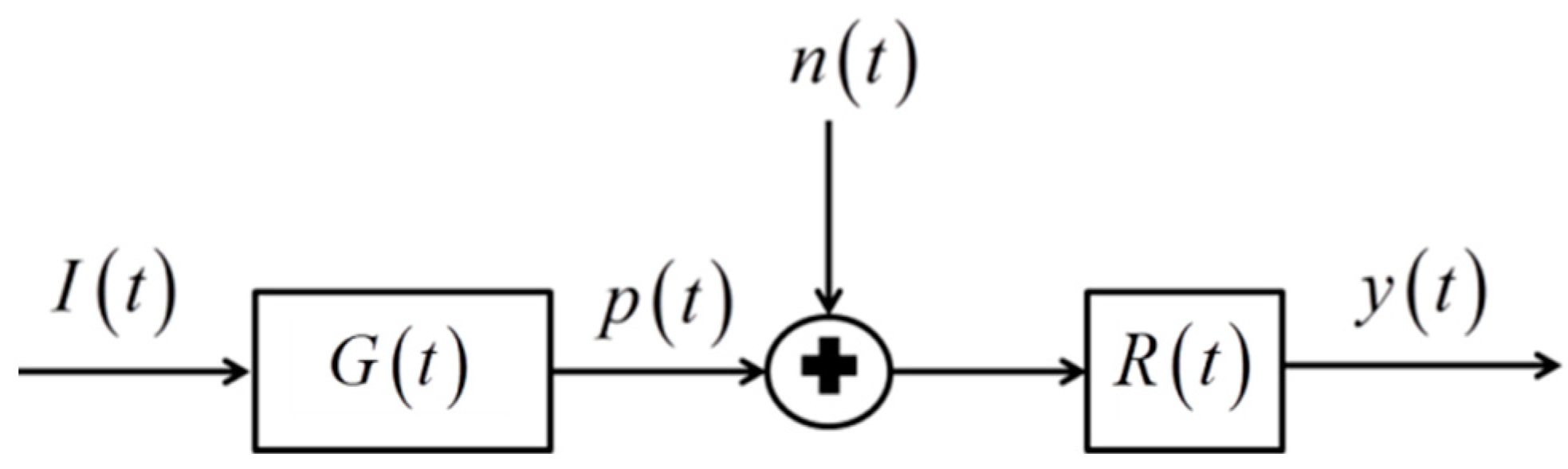
2. Mathematical Statement of the Problem

We considered a one-dimensional photoacoustic system for our analysis. For a one-dimensional photoacoustic system, the absorbing material surrounded with the scattering medium was considered to have the simple layout shown in Figure 1.

The incident laser waveform $I\left(t\right)$ is transmitted from the negative side of $z$ axis, outside of the absorber. The absorber absorbs energy from the incident laser and generates a pressure response denoted by $p\left(z,t\right)$. The pressure response is then detected by a transducer and be sent to a receiver-filter. The output of the receiver-filter $y\left(z,t\right)$ is the final photoacoustic signal.

Diebold [25] provided a concise explanation of the governing equation for the pressure that results from launching a photoacoustic wave, given by

$$\left[{\nabla }^2-\frac{1}{c_s^2}\frac{{\partial }^2}{\partial t^2}\right]p\left(\overrightarrow{r},t\right)=-\frac{\beta }{C_p}\frac{\partial H(\overrightarrow{r},t)}{\partial t}$$

(1)

where $\beta$ is the thermal expansion coefficient, $c_s$ is the speed of sound, $C_p$ is the specific heat, $H(\overrightarrow{r},t)$ is the energy per unit volume and time deposited by the optical radiation beam, and $p(\overrightarrow{r},t)$ is the pressure of the acoustic wave, a function of space and time.

In this work, it was assumed that the heating function $H(\overrightarrow{r},t)$ results from a chromophore absorber that is optically thin with an optical absorption coefficient ${\mu }_a$ that is heated by an optical pulse with a fluence of $F$. We assumed that $H(\overrightarrow{r},t)$ is a separable function of space and time so that the preceding assumptions imply that $H(\overrightarrow{r},t)={\mu }_{a}FA\left(\overrightarrow{r}\right)I\left(t\right)$. $A\left(\overrightarrow{r}\right)$ is a function of space that describes the geometry of the absorber and $I\left(t\right)$ is a function that describes the time dependence of the incident optical wave, as shown schematically in Figure 1. It has been shown [18] that in the frequency domain

$$\tilde{p}\left(z,f\right)=\tilde{G}\left(z,f\right)\tilde{I}\left(f\right)$$

(2)

where the transfer function is given by

$$\tilde{G}\left(z,f\right)=\frac{p_0}{2c_s}\{\begin{array}{c}\widehat{A}\left(-k\right)e^{-ikz}\hspace{0.17em}\hspace{0.17em}\hspace{0.17em}\hspace{0.17em}\hspace{0.17em}z>0\\ \widehat{A}\left(k\right)e^{ikz}\hspace{0.17em}\hspace{0.17em}\hspace{0.17em}\hspace{0.17em}\hspace{0.17em}\hspace{0.17em}\hspace{0.17em}\hspace{0.17em}\hspace{0.17em}z<0\end{array}$$

(3)

and $k=2\pi f/c_s$. Hence, the transfer function is, unsurprisingly, completely controlled by the shape of the absorber, $\widehat{A}\left(k\right)$. Therefore, the photoacoustic system can be modeled the same as many other detection or imaging systems, [19,26,27,28,29,30], in an input/output form as shown in Figure 2. The measurements are made at fixed points, so G and p will be functions of time only.

In Figure 2, $n\left(t\right)$ represents the noise in the system and $R\left(t\right)$ is the receiver-filter impulse response.

As shown in Figure 2, the output of the receiver-filter is given by

$$y\left(t\right)=y_s\left(t\right)+y_n\left(t\right)$$

(4)

where $y_s\left(t\right)$ is informative signal part of the pressure response, and $y_n\left(t\right)$ is the noise component. The pressure response signal can be expressed as

$$y_s\left(t\right)=I\left(t\right)\ast G\left(t\right)\ast R\left(t\right)$$

(5)

where * denotes convolution. The noise part is then given by

$$y_n\left(t\right)=R\left(t\right)\ast n\left(t\right)$$

(6)

where the noise is assumed to be stationary and ergodic and to have a double-sided power spectral density of $S_{nn}\left(f\right)=N_0/2$.

2.1. Maximizing SNR

The maximum signal-to-noise ratio (SNR) at time $t_0$ will be given by [19]

$${\left(\frac{S}{N}\right)}_{t_0}=\frac{{\left|y_s\left(t_0\right)\right|}^2}{E{\left|y_n\left(t_0\right)\right|}^2}$$

(7)

where $E{\left|y_n\left(t_0\right)\right|}^2$ is the expectation of noise power at time $t_0$.

The numerator of the SNR expression in Equation (7) can be written via frequency domain quantities as

$${\left|y_s\left(t_0\right)\right|}^2={\left|{\displaystyle \underset{-\infty }{\overset{\infty }{\int }}\tilde{I}\left(f\right)\tilde{G}\left(f\right)\tilde{R}\left(f\right)e^{2\pi if{t}_0}}df\right|}^2$$

(8)

where the tilde indicates a temporal Fourier transform of the indicated function. The denominator is

$$\begin{array}{c}E{\left|y_n\left(t_0\right)\right|}^2=E\left\{y_n\left(t_0\right)\overline{y_n\left(t_0\right)}\right\}\\ =R_{y_n{y}_n}\left(t_0\right)\\ ={\displaystyle {\int }_{-\infty }^{\infty }{\left|\tilde{R}\left(f\right)\right|}^2{S}_{nn}\left(f\right)}{e}^{2\pi if{t}_0}df\end{array}$$

(9)

Here, the bar on $\overline{y_n\left(t_0\right)}$ denotes complex conjugate, and $R_{y_n{y}_n}\left(t_0\right)$ is the autocorrelation function of $y_n\left(t\right)$. Therefore, Equation (7) for the SNR becomes

$${\left(\frac{S}{N}\right)}_{t_0}=\frac{{\left|{\displaystyle \underset{-\infty }{\overset{\infty }{\int }}\tilde{I}\left(f\right)\tilde{G}\left(f\right)\tilde{R}\left(f\right)e^{2\pi if{t}_0}}df\right|}^2}{{\displaystyle {\int }_{-\infty }^{\infty }{\left|\tilde{R}\left(f\right)\right|}^2{S}_{nn}\left(f\right)} e^{2\pi if{t}_0}df}$$

(10)

This can be written as

$${\left(\frac{S}{N}\right)}_{t_0}=\frac{{\left|{\displaystyle \underset{-\infty }{\overset{\infty }{\int }}\left[\frac{\tilde{I}\left(f\right)\tilde{G}\left(f\right)e^{2\pi if{t}_0}}{\sqrt{S_{nn}\left(f\right)}}\right]\left[\tilde{R}\left(f\right)\sqrt{S_{nn}\left(f\right)}\right]}df\right|}^2}{{\displaystyle {\int }_{-\infty }^{\infty }{\left|\tilde{R}\left(f\right)\right|}^2{S}_{nn}\left(f\right)}{e}^{2\pi if{t}_0}df}$$

(11)

Applying the Schwartz inequality [31] to the numerator gives

$$\begin{array}{c}{\left|{\displaystyle \underset{-\infty }{\overset{\infty }{\int }}\left[\frac{\tilde{I}\left(f\right)\tilde{G}\left(f\right)e^{2\pi if{t}_0}}{\sqrt{S_{nn}\left(f\right)}}\right]\left[\tilde{R}\left(f\right)\sqrt{S_{nn}\left(f\right)}\right]}df\right|}^2\\ \le {\displaystyle \underset{-\infty }{\overset{\infty }{\int }}\frac{{\left|\tilde{I}\left(f\right)\tilde{G}\left(f\right)\right|}^2}{S_{nn}\left(f\right)}}df{\displaystyle \underset{-\infty }{\overset{\infty }{\int }}{\left|\tilde{R}\left(f\right)\right|}^2{S}_{nn}\left(f\right)}df\hfill \end{array}$$

(12)

Equality follows if and only if [31]

$$\tilde{R}\left(f\right)\sqrt{S_{nn}\left(f\right)}=K\overline{\left[\frac{\tilde{I}\left(f\right)\tilde{G}\left(f\right)e^{2\pi if{t}_0}}{\sqrt{S_{nn}\left(f\right)}}\right]}$$

(13)

where K is a complex proportionality constant and assumed to be one for calculation convenience. Equivalently,

$$\tilde{R}\left(f\right)=K\frac{\overline{\tilde{I}\left(f\right)\tilde{G}\left(f\right)}}{S_{nn}\left(f\right)}{e}^{-2\pi if{t}_0}$$

(14)

where $\tilde{R}\left(f\right)$ is often referred to as Matched-Filter [32,33]. Thus, we have

$$\begin{array}{c}{\left(\frac{S}{N}\right)}_{t_0}\le \frac{{\displaystyle \underset{-\infty }{\overset{\infty }{\int }}\frac{{\left|\tilde{I}\left(f\right)\tilde{G}\left(f\right)\right|}^2}{S_{nn}\left(f\right)}}df{\displaystyle \underset{-\infty }{\overset{\infty }{\int }}{\left|\tilde{R}\left(f\right)\right|}^2{S}_{nn}\left(f\right)}df}{{\displaystyle \underset{-\infty }{\overset{\infty }{\int }}{\left|\tilde{R}\left(f\right)\right|}^2{S}_{nn}\left(f\right)}df}\\ ={\displaystyle \underset{-\infty }{\overset{\infty }{\int }}\frac{{\left|\tilde{I}\left(f\right)\tilde{G}\left(f\right)\right|}^2}{S_{nn}\left(f\right)}}df\end{array}$$

(15)

where equality follows if and only if Equation (14) holds.

Hence, the maximum possible SNR is given by Equation (15), and the general problem of interest is how can we select the input waveform so that the value of the maximum SNR is itself maximized.

2.2. Maximizing SNR under Constraints on the Input

The problem of maximizing the SNR under constraints on the input waveform energy and duration can be stated as maximizing

$$SN{R}_{\max }={\displaystyle \underset{-\infty }{\overset{\infty }{\int }}\frac{{\left|\tilde{I}\left(f\right)\tilde{G}\left(f\right)\right|}^2}{S_{nn}\left(f\right)}}df$$

(16)

under energy and duration constraints of the input written as

$$\begin{array}{l}{\displaystyle \underset{-\infty }{\overset{\infty }{\int }}{\left|\tilde{I}\left(f\right)\right|}^2}df=E,\\ I\left(t\right)=0, for all t\notin \left[-T/2, T/2\right]\end{array}$$

(17)

Here, we have assumed that there is a maximum allowable energy of the input waveform, given by E, and a maximum allowable duration of the input waveform given by T.

We can write (16) as

$$\begin{array}{c}SN{R}_{\max }={\displaystyle \underset{-\infty }{\overset{\infty }{\int }}{\left|\tilde{I}\left(f\right)\left[\frac{\tilde{G}\left(f\right)}{\sqrt{S_{nn}\left(f\right)}}\right]\right|}^2}df\\ ={\displaystyle \underset{-\infty }{\overset{\infty }{\int }}{\left|\tilde{I}\left(f\right)\tilde{B}\left(f\right)\right|}^2}df\end{array}$$

(18)

where

$$\tilde{B}\left(f\right)=\frac{\tilde{G}\left(f\right)}{\sqrt{S_{nn}\left(f\right)}}$$

(19)

Maximizing Equation (18) is equivalent to maximizing an integral of the form

$${\displaystyle \underset{-\infty }{\overset{\infty }{\int }}{\left|q\left(t\right)\right|}^2}dt={\displaystyle \underset{-\infty }{\overset{\infty }{\int }}{\left|\tilde{q}\left(f\right)\right|}^2}df={\displaystyle \underset{-\infty }{\overset{\infty }{\int }}{\left|\tilde{I}\left(f\right)\tilde{B}\left(f\right)\right|}^2}df$$

(20)

Then, using the constraint on waveform duration and rewriting the Fourier transform of the input waveform in terms of its definition, this becomes

$${\displaystyle \underset{-\infty }{\overset{\infty }{\int }}{\left|q\left(t\right)\right|}^2}dt={\displaystyle \underset{-\infty }{\overset{\infty }{\int }}\left[{\displaystyle \underset{-T/2}{\overset{T/2}{\int }}I\left(\tau \right)e^{-2\pi if\tau }}d\tau \right]\left[{\displaystyle \underset{-T/2}{\overset{T/2}{\int }}\overline{I\left(p\right)}{e}^{2\pi ifp}}dp\right]{\left|\tilde{B}\left(f\right)\right|}^2}df$$

(21)

We note that the input waveform must be real. Now define $L\left(t\right)$ as the inverse Fourier transform of ${\left|\tilde{B}\left(f\right)\right|}^2$

$$L\left(t\right)\triangleq {\displaystyle \underset{-\infty }{\overset{\infty }{\int }}{\left|\tilde{B}\left(f\right)\right|}^2}{e}^{2\pi ift}df$$

(22)

Then, by interchanging the order of the integration, Equation (21) can be written as

$${\displaystyle \underset{-\infty }{\overset{\infty }{\int }}{\left|q\left(t\right)\right|}^2}dt={\displaystyle \underset{-T/2}{\overset{T/2}{\int }}{\displaystyle \underset{-T/2}{\overset{T/2}{\int }}\overline{I\left(p\right)}I\left(\tau \right)L\left(p-\tau \right)}}d\tau dp$$

(23)

It then follows that the optimum function $\widehat{I}\left(t\right)$ that maximizes (23) is given by

$$\lambda \widehat{I}\left(p\right)={\displaystyle \underset{-T/2}{\overset{T/2}{\int }}\widehat{I}\left(\tau \right)L\left(p-\tau \right)}d\tau$$

(24)

where $\lambda$ is the maximum eigenvalue of (24). $\widehat{I}\left(t\right)$ is an eigenfunction of Equation (24) corresponding to $\lambda$ and having energy E.

From (23) and (24), it would then follow that

$$\begin{array}{c}{\displaystyle \underset{-\infty }{\overset{\infty }{\int }}{\left|q\left(t\right)\right|}^2}dt={\displaystyle \underset{-T/2}{\overset{T/2}{\int }}\overline{\widehat{I}\left(p\right)}{\displaystyle \underset{-T/2}{\overset{T/2}{\int }}\widehat{I}\left(\tau \right)L\left(p-\tau \right)}}\hspace{0.17em}d\tau \hspace{0.17em}dp\\ \hspace{0.17em}\hspace{0.17em}\hspace{0.17em}\hspace{0.17em}\hspace{0.17em}\hspace{0.17em}\hspace{0.17em}\hspace{0.17em}\hspace{0.17em}\hspace{0.17em}\hspace{0.17em}\hspace{0.17em}\hspace{0.17em}\hspace{0.17em}\hspace{0.17em}={\displaystyle \underset{-T/2}{\overset{T/2}{\int }}\overline{\widehat{I}\left(p\right)}\lambda \widehat{I}\left(p\right)}\hspace{0.17em}dp\hfill \\ \hspace{0.17em}\hspace{0.17em}\hspace{0.17em}\hspace{0.17em}\hspace{0.17em}\hspace{0.17em}\hspace{0.17em}\hspace{0.17em}\hspace{0.17em}\hspace{0.17em}\hspace{0.17em}\hspace{0.17em}\hspace{0.17em}\hspace{0.17em}\hspace{0.17em}=\lambda {\displaystyle \underset{-T/2}{\overset{T/2}{\int }}{\left|\widehat{I}\left(p\right)\right|}^2}dp\hfill \\ \hspace{0.17em}\hspace{0.17em}\hspace{0.17em}\hspace{0.17em}\hspace{0.17em}\hspace{0.17em}\hspace{0.17em}\hspace{0.17em}\hspace{0.17em}\hspace{0.17em}\hspace{0.17em}\hspace{0.17em}\hspace{0.17em}\hspace{0.17em}\hspace{0.17em}=\lambda E\hfill \end{array}$$

(25)

Hence, the maximum SNR is given by the solution to the integral eigenvalue problem given by

$${\lambda }_{\max }\widehat{I}\left(t\right)={\displaystyle \underset{-T/2}{\overset{T/2}{\int }}\widehat{I}\left(\tau \right)L\left(t-\tau \right)}d\tau$$

(26)

Equation (26) is a Fredholm integral equation of the second kind. $L\left(t\right)$ is known as the kernel of the integral. In the following subsections, we examine three different types of kernels derived from three different absorber profiles and consider the consequences.

3. Numerical Simulations

To show that Equation (26) holds true, simulations were performed with bandlimited, square, and Gaussian absorber profiles. In the following subsections, we introduce the mathematical formulations for these three absorbers. These three absorbers were chosen because (i) the bandlimited absorber can investigate the general limitation on bandlimits, either from the absorber itself or arising from instrumentation; (ii) the square absorber is space-limited and finite in space, and it can be used to investigate the effects of limitations in space; and (iii) the Gaussian absorber is neither space nor bandlimited and we can thus examine what happens when there are not hard limits in space or frequency.

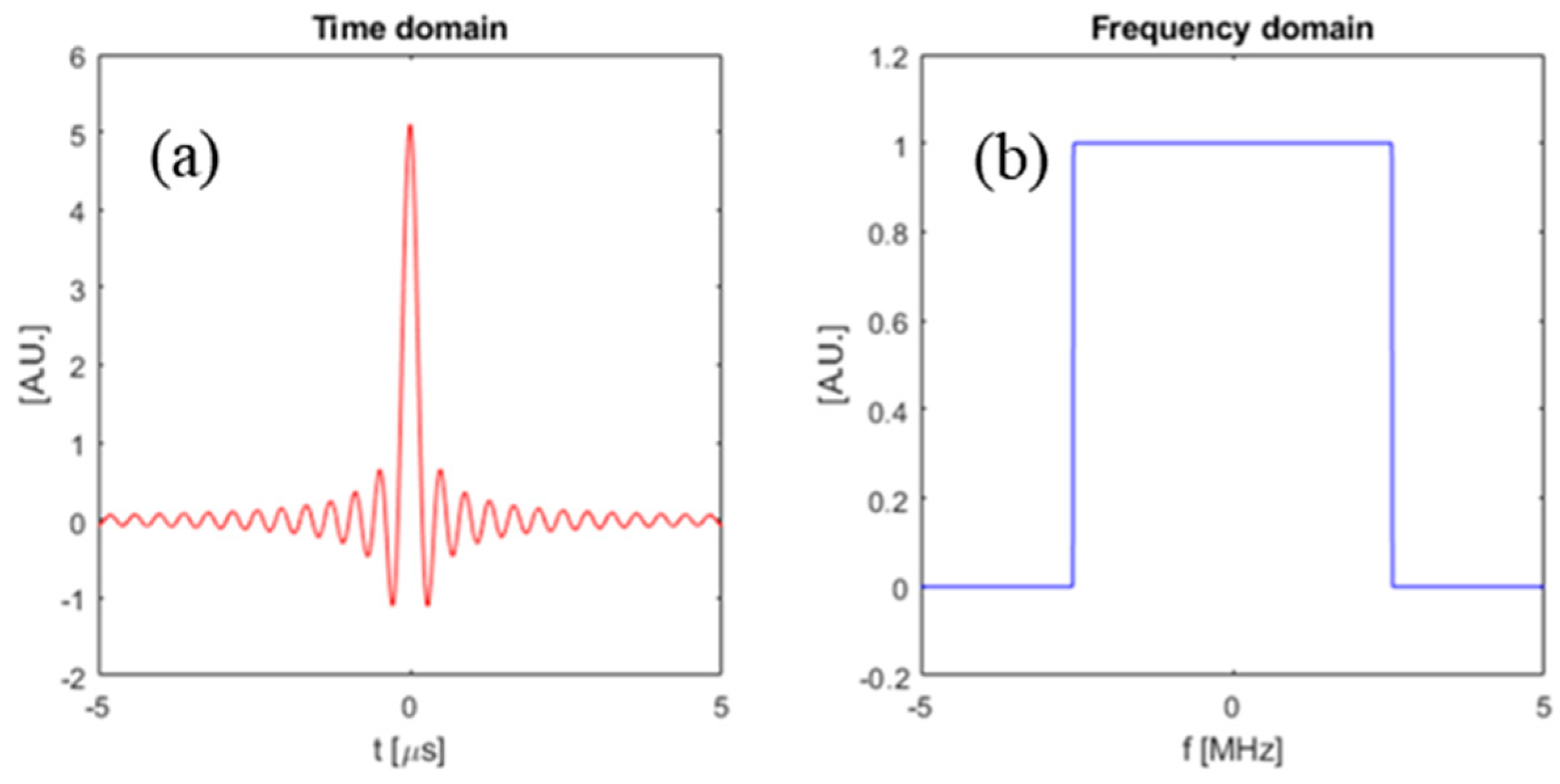
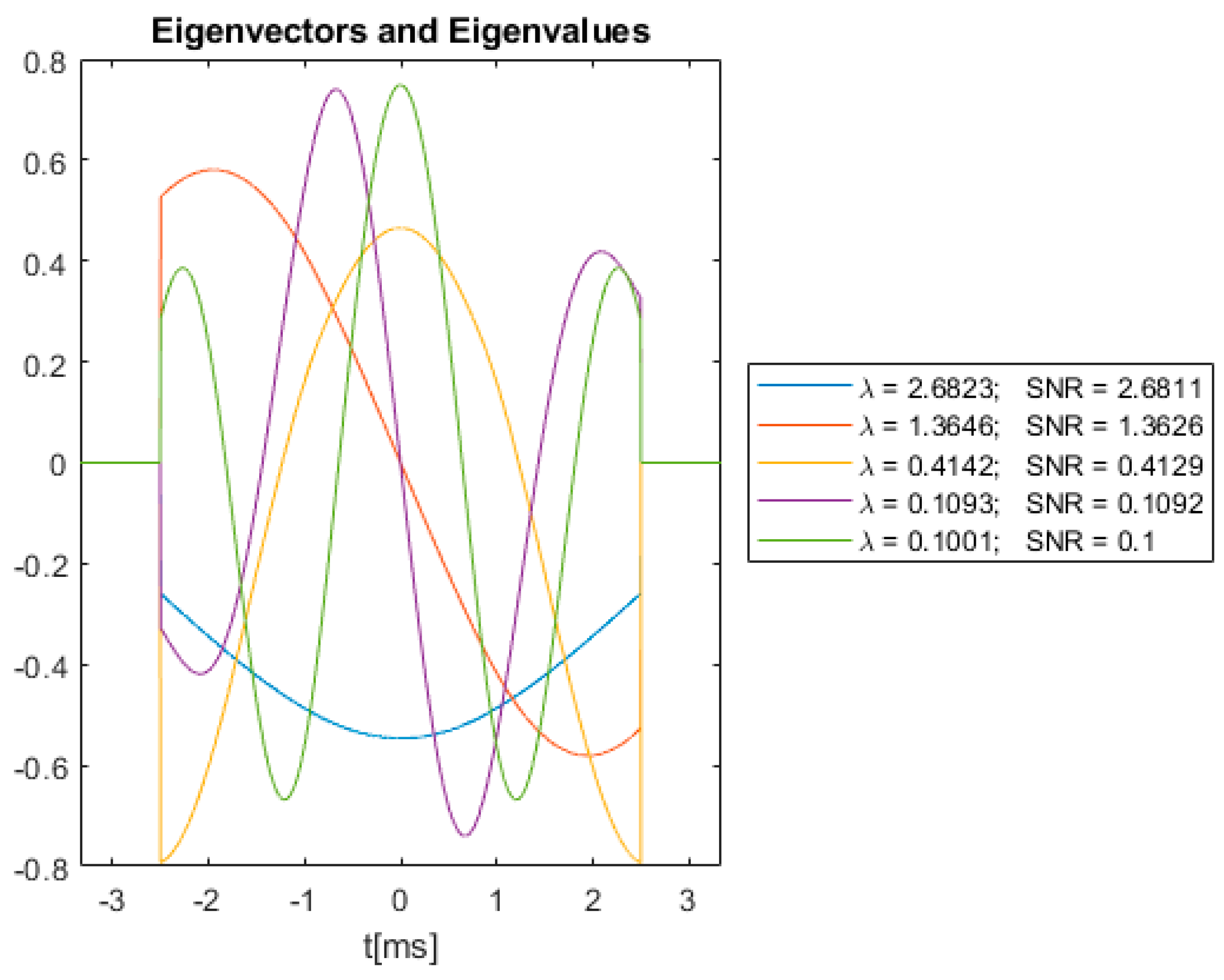
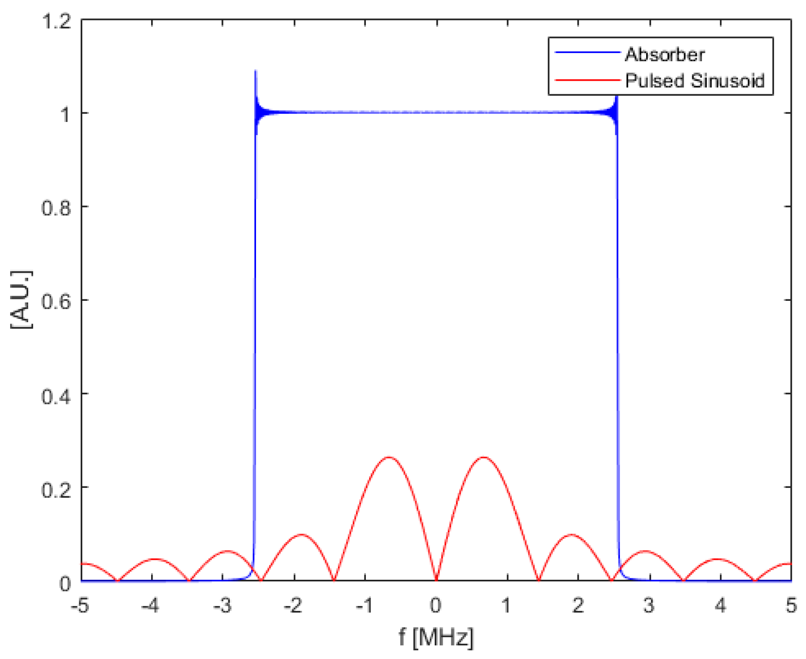
3.1. Bandlimited Absorber

A bandlimited absorber is defined as a rectangular function in frequency as

$$\tilde{G}\left(f\right)=\{\begin{array}{l}1, \left|f\right|\le {\Delta }_a\\ 0, Otherwise\end{array}$$

(27)

where ${\Delta }_a$ is the bandwidth of absorber. A plot of the bandlimited absorber with ${\Delta }_a=2.55\mathrm{MHz}$ is shown in Figure 3.

The kernel in (26) for a bandlimited absorber will be a sinc function,

$$L\left(t\right)=2{\Delta }_a\frac{\sin \left(2\pi {\Delta }_{a}t\right)}{2\pi {\Delta }_{a}t}$$

(28)

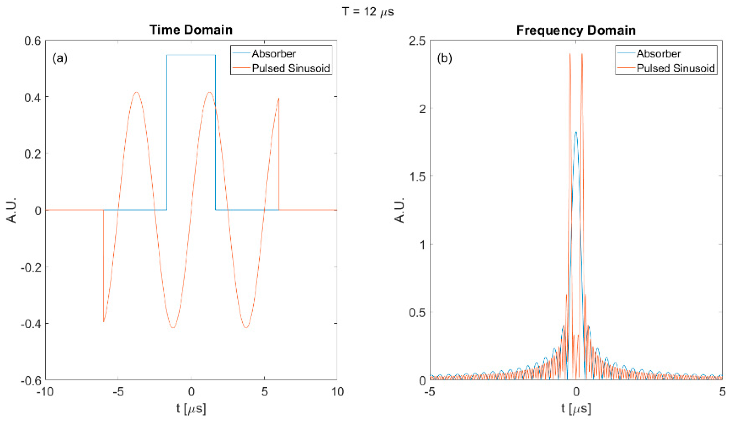
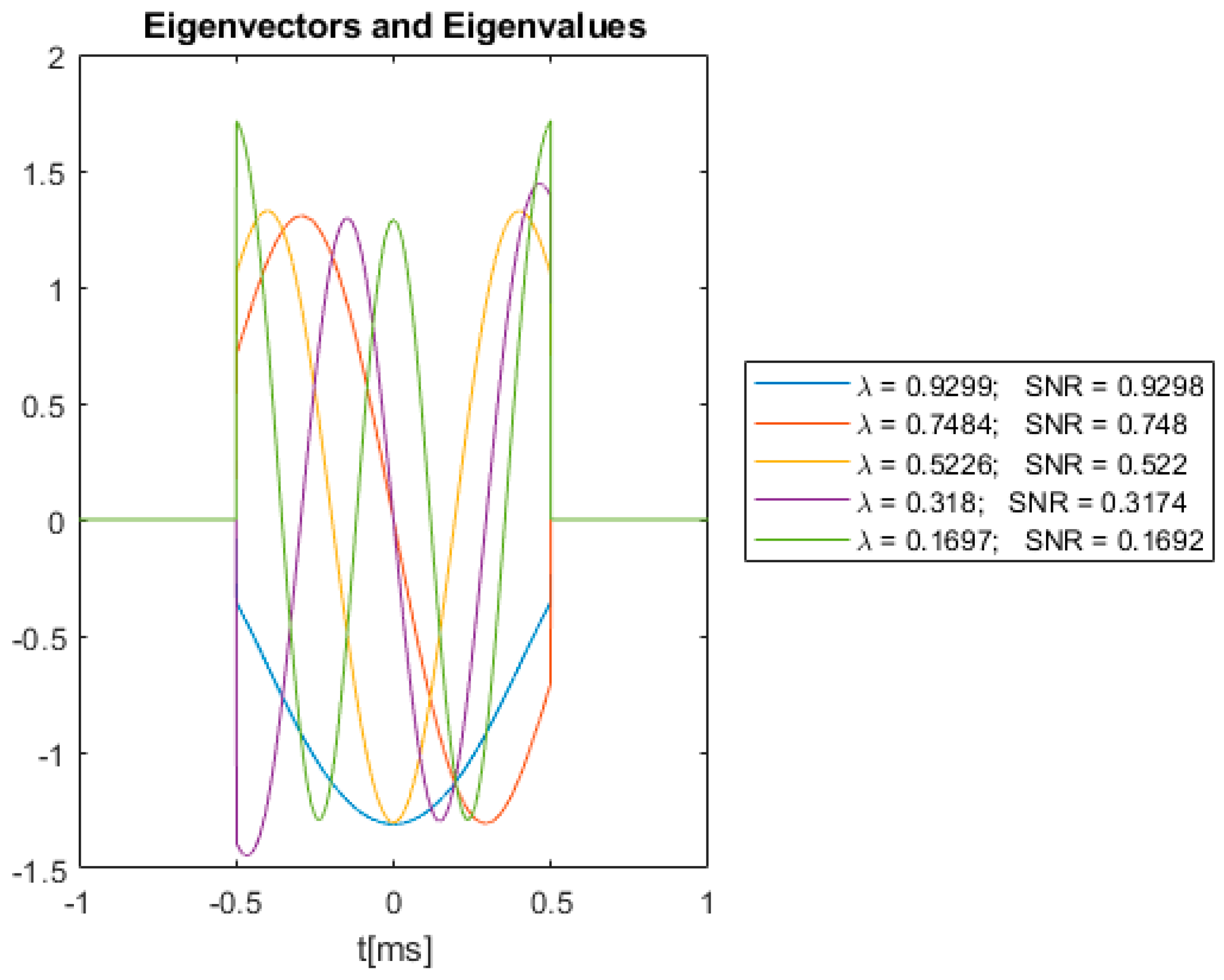
3.2. Square Absorber

A square absorber of length $l$ in space can be defined as a rectangular function in time with a converting factor for the speed of sound, $c_s$, inside the absorber. The speed of sound in human tissue can be approximated by $c_s=1500 \mathrm{m}/\mathrm{s}$ [34], and a typical absorber thickness is several millimeters [14,18,35]. A one-dimensional square absorber in space can thus be converted to an equivalent square absorber in time by using the speed of sound in the absorber.

$$G\left(t\right)=\{\begin{array}{l}\sqrt{\frac{c_s}{l}}, \left|t\right|\le \frac{l}{2c_s}\\ 0, Otherwise\end{array}$$

(29)

where $c_s$ is the speed of sound in absorber and $l$ is the thickness of absorber. The magnitude of the square absorber is normalized to $\sqrt{c_s/l}$ for calculation convenience in what follows, but can have any magnitude without affecting the validity of the results. A plot of a square absorber with $l=5$ mm and $c_s=1500 \mathrm{m}/\mathrm{s}$ is shown in Figure 4.

The kernel in (26) with a square absorber given by (29) will be a triangle function,

$$L\left(t\right)=\{\begin{array}{l}\left(1-\frac{l}{c_s}\right)\left|t\right|, \left|t\right|\le \frac{l}{c_s}\\ 0, Otherwise\end{array}$$

(30)

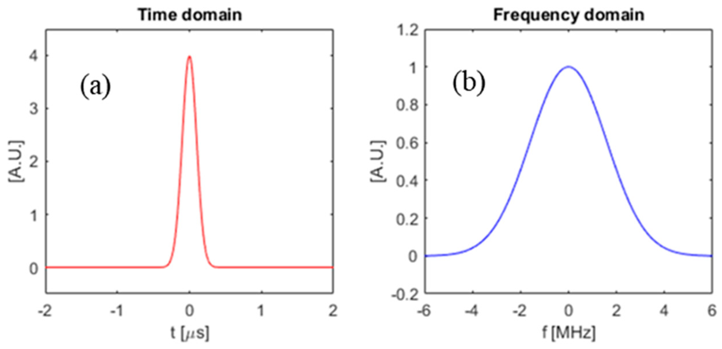
3.3. Gaussian Absorber

Now consider a more realistic absorber shape, the Gaussian absorber. If the absorber has a Gaussian shape in time with its mean at 0, then the impulse response is given by

$$G\left(t\right)=\frac{e^{-\frac{t^2}{2{\sigma }^2}}}{\sigma \sqrt{2\pi }}$$

(31)

Similar to the square absorber, which is absorbing light uniformly, the light absorption in Gaussian absorber can be considered as inhomogeneous and have a Gaussian profile along the thickness of absorber. $\sigma$ is the standard deviation that defines the width of the Gaussian absorber. A larger $\sigma$ means a thicker absorber in time or equivalently, space. Full Width Half Maximum (FWHM) of an absorber with Gaussian absorbance profile is approximately $2.355\sigma \left[\mathsf{\mu }\mathrm{s}\right]$ [36] or this can be converted to the equivalent space dimension via the speed of sound in the absorber as $2.355\sigma \cdot c_s\left[\mathsf{\mu }\mathrm{m}\right]$.

A plot of a Gaussian absorber with $\sigma =0.1 \mathsf{\mu }\mathrm{s}$ is shown in Figure 5.

The kernel in (26) will still be a Gaussian function but widened,

$$L\left(t\right)=\frac{e^{-\frac{t^2}{4{\sigma }^2}}}{2\sigma \sqrt{\pi }}$$

(32)

3.4. Optimal SNR and Eigenvalue

Simulations on SNR were performed with the three absorbers in this section. Figure 6 shows the eigenvectors obtained by solving (26) with the kernel defined in (28), for the bandlimited absorber. The bandwidth of the absorber is chosen as ${\Delta }_a=2.55 \mathrm{MHZ}$.

Figure 7 shows the eigenvectors obtained by solving (26) with the kernel defined in (30) for the square absorber.

Figure 8 shows the eigenvectors obtained by (26) with the kernel defined in (32) for the Gaussian absorber.

In Figure 6, Figure 7 and Figure 8, the eigenfunctions are scaled to have unit energy. Hence, according to (25), the SNRs will have the same value as the eigenvalues. The SNR values in the legends are obtained using Equation (10) with $I\left(t\right)$ chosen to be the eigenvectors shown in Figure 6, Figure 7 and Figure 8, receiver-filter $\tilde{R}\left(f\right)=\overline{\tilde{I}\left(f\right)\tilde{G}\left(f\right)}$ and the assumption that $S_{nn}\left(f\right)=N_0/2=1$.

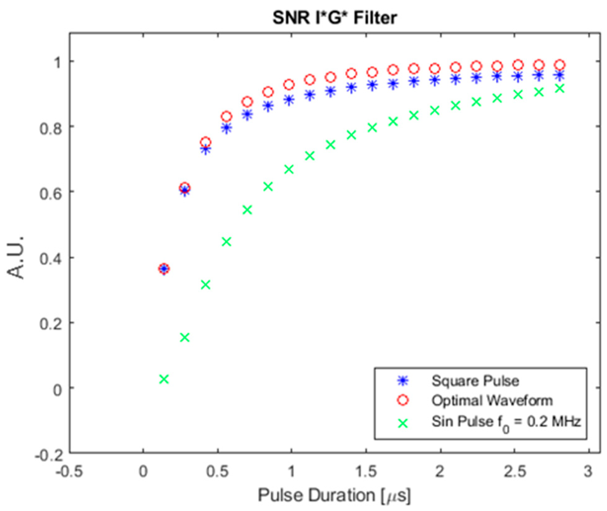
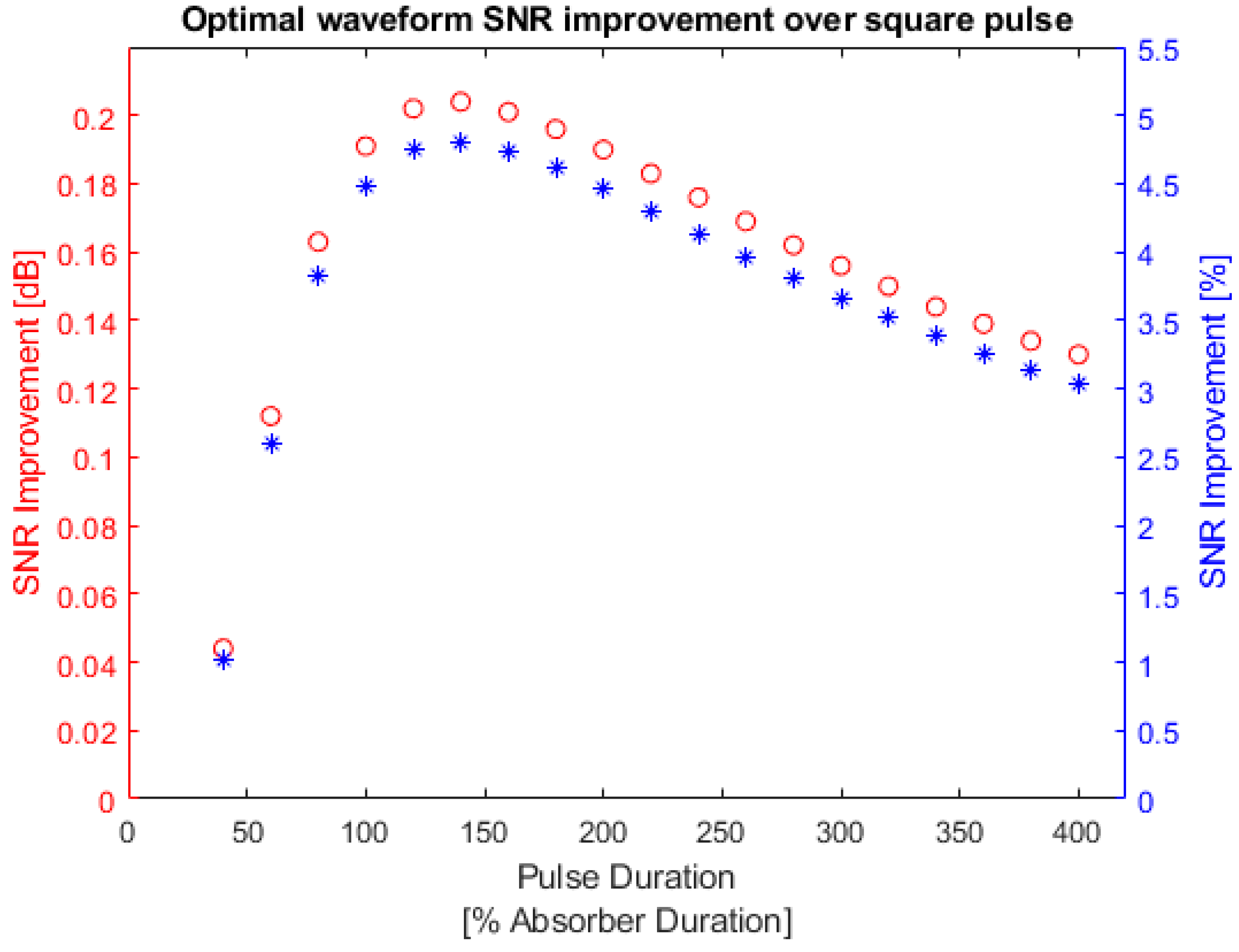
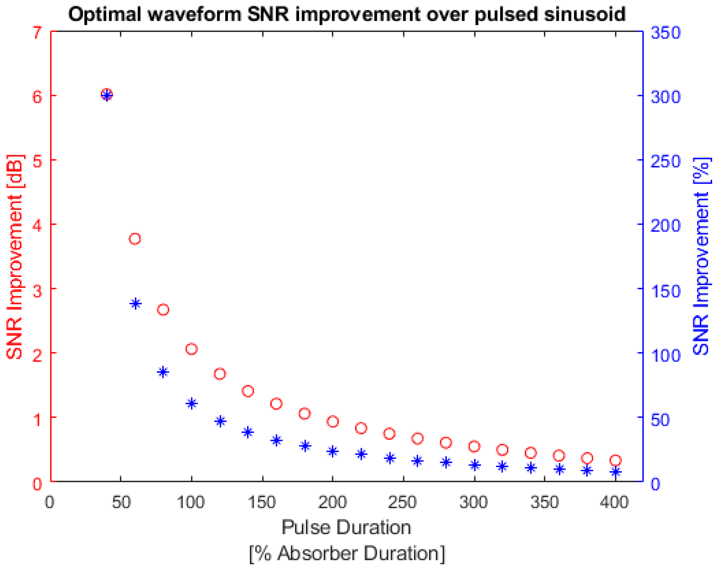
3.5. SNR Comparison between Different Input Waveforms

In this section, we compare the SNR gains that can be obtained by using the optimal waveform from the previous section as compared to some other waveforms. Specifically, we compare the SNR between three chosen input waveforms: (i) the optimal waveform obtained using the method in Section 2, (ii) a simple square pulse, and (iii) a pulsed sinusoid. The square pulse is defined as a rectangle function in time with duration T, and the pulsed sinusoid is defined as a single-frequency sine function truncated with a square window to have duration T. Figure 9 shows a square pulse with $T=10\hspace{0.17em}\mathsf{\mu }\mathrm{s}$, and also a pulsed sinusoid with $T=10\hspace{0.17em}\mathsf{\mu }\mathrm{s}$ with carrier frequency $f_0=\hspace{0.17em}0.2\mathrm{MHz}$. Figure 10 is the frequency domain plot of the input waveforms shown in Figure 9.

As shown in Figure 6, Figure 7 and Figure 8, Equation (24) can yield multiple eigenfunctions and eigenvalues. However, the optimal waveform will be the eigenfunction associated with the largest eigenvalue, which are the blue curves in Figure 6, Figure 7 and Figure 8. This will yield the highest possible SNR for the absorbers associated with Figure 6, Figure 7 and Figure 8.

SNRs obtained with different input waveforms in the simulation were calculated from Equation (10) with $I\left(t\right)$ chosen to be the eigenvectors obtained from (26) for optimal waveform, and input waveforms shown in Figure 9. All input waveforms were scaled to have unit energy. The receiver-filter in Equation (10) is $\tilde{R}\left(f\right)=\overline{\tilde{I}\left(f\right)\tilde{G}\left(f\right)}$ and we assumed $S_{nn}\left(f\right)=N_0/2=1$. In the SNR improvement figures, SNR is converted to decibels using

$${SNR|}_{dB}=10{\log }_{10}\left(SNR\right)$$

(33)

The SNR difference was calculated with

$$10{\log }_{10}\left({SNR|}_{Optimal waveform}\right)-10{\log }_{10}\left({SNR|}_{Other waveform}\right)$$

(34)

The SNR improvement in percentage was calculated from

$$\frac{{SNR|}_{Optimal waveform}-{SNR|}_{Other waveform}}{{SNR|}_{Other waveform}}\times 100\%$$

(35)

3.5.1. Bandlimited Absorber SNR

SNRs for the bandlimited absorber shown in Figure 3 with optimal, square-pulse, and pulsed sinusoid input waveforms with various input pulse durations were calculated from Equation (10) and plotted in Figure 11. The horizontal axis in Figure 11 shows the input pulse duration and the vertical axis shows SNR values before taking the logarithm.

As shown in Figure 11, the optimal waveform always provides a higher SNR than the other two waveforms, in accordance with our proposed approach. Figure 12 shows the SNR improvement by comparing the optimal waveform and the square pulse waveform. The horizontal axis is taken to be the percentage of the absorber effective duration to show the relation between SNR improvement and the input pulse relative duration, in comparison to the duration of the absorber. The effective duration of the bandlimited absorber is taken to be the main peak width defined by the 1st zero crossings of the sinc function in time, $T_{effective}=0.392\hspace{0.17em}\mu s$.

As shown in Figure 12 the SNRs of the optimal waveform were always higher than the other waveforms, especially when the pulse durations were comparable to the effective duration of the absorber (the input waveform is around 120% of the absorber effective duration). SNR values and improvements in Figure 11 and Figure 12 are shown in Appendix A 

Table A1. SNR comparison between optimal waveform and square pulse waveform with bandlimited absorber.

T (us)	SNR Optimal	SNR Pulse	SNR Improvement (%)	SNR Improvement (dB)
0.157	0.658	0.676	2.59	0.114
0.235	0.85	0.839	1.275	0.055
0.314	0.944	0.896	5.33	0.226
0.392	0.982	0.903	8.73	0.363
0.471	0.995	0.907	9.749	0.404
0.549	0.999	0.922	8.39	0.35
0.627	1	0.939	6.492	0.273
0.706	1	0.948	5.478	0.232
0.784	1	0.95	5.315	0.225
0.863	1	0.951	5.192	0.22
0.941	1	0.956	4.65	0.197
1.02	1	0.962	3.959	0.169
1.098	1	0.966	3.563	0.152
1.176	1	0.966	3.494	0.149
1.255	1	0.967	3.439	0.147
1.333	1	0.969	3.184	0.136
1.412	1	0.972	2.842	0.122
1.49	1	0.974	2.636	0.113
1.569	1	0.975	2.599	0.111

. The maximum SNR improvement over a square pulse that can be achieved by using the optimal waveform was 9.749%.

Figure 13 shows the SNR improvement that can be achieved by using the optimal waveform instead of the pulsed sinusoid waveform.

In Figure 13, the pulsed sinusoid waveform shows a very low SNR compared with the optimal waveform. This is because the pulsed sinusoid uses a 0.2 MHz carrier frequency which shifts its peak in frequency domain to be centered at 0.2 MHz. The pulsed sinusoid waveform spreads its energy in a wider frequency range outside of the absorber bandwidth, as shown in Figure 14, which contributes to the lower SNR values.

Table A2. SNR comparison between optimal waveform and pulsed sinusoid waveform with the bandlimited absorber.

T (us)	SNR Optimal	SNR Pulsed Sinusoid	SNR Improvement (%)	SNR Improvement (dB)
0.157	0.658	0.116	466.904	7.535
0.235	0.85	0.31	174.117	4.379
0.314	0.944	0.533	77.093	2.482
0.392	0.982	0.701	40.071	1.463
0.471	0.995	0.778	27.862	1.067
0.549	0.999	0.793	26.016	1.004
0.627	1	0.797	25.465	0.985
0.706	1	0.82	22.035	0.865
0.784	1	0.853	17.327	0.694
0.863	1	0.876	14.257	0.579
0.941	1	0.882	13.366	0.545
1.02	1	0.884	13.135	0.536
1.098	1	0.892	12.114	0.497
1.176	1	0.906	10.428	0.431
1.255	1	0.917	9.115	0.379
1.333	1	0.921	8.632	0.36
1.412	1	0.922	8.475	0.353
1.49	1	0.926	7.979	0.333
1.569	1	0.934	7.119	0.299

in Appendix A lists the SNR values of the optimal waveform and the pulsed sinusoid. The maximum SNR improvement can be achieved in the simulation was 466.904%. However, this large improvement was obtained when the pulse duration was extremely small so that the pulsed sinusoid could not have a complete cycle.

3.5.2. Square Absorber SNR

Figure 15 shows the SNR for a square absorber shown in Figure 4 using the three different input waveforms.

As shown in Figure 15, a similar trend was observed. The optimal waveform always provided higher SNR than the other two waveforms. However, the SNR of the pulsed sinusoid waveform was extremely low compared with the other two waveforms. This can be explained in Figure 16. Figure 16 shows the time and frequency domain plot of the square absorber and a pulsed sinusoid with 1 μs duration.

As shown in Figure 16, the square absorber in the frequency domain is a sinc function with its main peak centered at zero frequency. However, the pulsed sinusoid with carrier frequency $f_0=0.2 \mathrm{MHz}$ concentrates most of its energy outside the main peak of absorber. Hence, the absorber could not react with the input waveform and generated a relatively low SNR. The increasing–decreasing (‘wavy’) phenomenon for the SNR of the pulsed sinusoid waveform in Figure 15 is also caused by the frequency domain profile of the input waveform. A detailed explanation is provided in Appendix B.

Similar to Figure 12, Figure 17 shows the SNR improvement by comparing the optimal waveform with the square pulse waveform. The left y-axis is the SNR improvement in decibels and the right y-axis is SNR improvement in percentages.

Similar to the bandlimited absorber, the optimal waveform for a square absorber showed a larger improvement when the pulse duration was comparable to the absorber effective duration. However, the largest improvement was observed when the pulse duration was around 250% of the absorber effective duration instead of 120% as was observed for the bandlimited absorber. This may be due to the fact that the square absorber has a clear definition of duration as shown in Figure 4, while the bandlimited absorber is a sinc function in time and has many sidelobes outside the defined effective duration.

Appendix A 

Table A3. SNR comparison between optimal waveform and square pulse waveform with the square absorber.

T (us)	SNR Optimal	SNR Pulse	SNR Improvement (%)	SNR Improvement (dB)
1.333	1.156	1.156	0.033	0.001
2	1.604	1.6	0.246	0.011
2.667	1.968	1.956	0.622	0.027
3.333	2.251	2.222	1.278	0.055
4	2.46	2.407	2.194	0.094
4.667	2.618	2.54	3.079	0.132
5.333	2.737	2.639	3.739	0.159
6	2.83	2.716	4.196	0.178
6.667	2.905	2.778	4.567	0.194
7.333	2.963	2.828	4.754	0.202
8	3.011	2.87	4.896	0.208
8.667	3.049	2.906	4.927	0.209
9.333	3.083	2.936	4.999	0.212
10	3.109	2.963	4.945	0.21
10.667	3.133	2.986	4.922	0.209
11.333	3.152	3.006	4.833	0.205
12	3.172	3.025	4.865	0.206
12.667	3.182	3.041	4.655	0.198
13.333	3.196	3.055	4.596	0.195

lists the SNR values between the optimal waveform and square-pulse waveform for a square absorber. From Table A3, the maximum improvement that could be achieved by using the optimal waveform instead of a square pulse was 4.999%.

Figure 18 shows the SNR improvement that can be achieved by using the optimal waveform instead of the pulsed sinusoid waveform for a square absorber.

Similar to the bandlimited absorber, SNR of the pulsed sinusoid is worse than a simple square pulse because the carrier frequency shifts its energy concentration outside of the absorber frequency spectrum so the absorber cannot react. Appendix A,

Table A4. SNR comparison between optimal waveform and pulsed sinusoid waveform with the square absorber.

T (us)	SNR Optimal	SNR Pulsed Sinusoid	SNR Improvement (%)	SNR Improvement (dB)
1.333	1.16	0.107	977.237	10.323
2	1.6	0.243	560.914	8.201
2.667	1.97	0.432	355.3	6.583
3.333	2.25	0.668	237.134	5.278
4	2.46	0.912	169.635	4.308
4.667	2.62	1.082	142.043	3.839
5.333	2.74	1.08	153.568	4.041
6	2.83	0.881	221.326	5.069
6.667	2.91	0.636	356.915	6.598
7.333	2.96	0.523	466.711	7.534
8	3.01	0.561	437.138	7.301
8.667	3.05	0.675	351.491	6.546
9.333	3.08	0.79	290.506	5.916
10	3.11	0.838	270.845	5.692
10.667	3.13	0.786	298.454	6.004
11.333	3.15	0.665	374.279	6.76
12	3.17	0.563	463.317	7.508
12.667	3.18	0.544	485.44	7.675
13.333	3.2	0.598	434.502	7.279

lists the SNR values for optimal waveform and the pulsed sinusoid waveform along with the improvement in both dB and percentage. The SNR improvement with any pulse duration is extremely large because the pulsed sinusoid concentrates its energy outside of the absorber bandwidth. The maximum SNR improvement is 977.237% which occurs at the shortest pulse duration.

3.5.3. Gaussian Absorber

Figure 19 shows the SNR for a Gaussian absorber using the three different input waveforms.

As shown in Figure 19, the optimal waveform always provided a higher SNR than the other two waveforms, especially when the pulse duration was comparable to the absorber duration, which was taken to be 0.7 μs for this Gaussian absorber. Figure 20 shows the SNR improvement in decibels and percentages against the pulse relative duration.

The same trend as before is also observed in Figure 20. The optimal waveform of the Gaussian absorber showed large improvements when the pulse duration was comparable to the absorber effective duration. Appendix A,

Table A5. SNR comparison between the optimal waveform and square pulse waveform with the Gaussian absorber.

T (us)	SNR Optimal	SNR Pulse	SNR Improvement (%)	SNR Improvement (dB)
0.28	0.612	0.606	1.021	0.044
0.42	0.751	0.732	2.606	0.112
0.56	0.829	0.798	3.832	0.163
0.7	0.876	0.839	4.487	0.191
0.84	0.907	0.866	4.755	0.202
0.98	0.927	0.885	4.806	0.204
1.12	0.942	0.899	4.74	0.201
1.26	0.952	0.91	4.615	0.196
1.4	0.96	0.919	4.46	0.19
1.54	0.967	0.927	4.295	0.183
1.68	0.971	0.933	4.128	0.176
1.82	0.975	0.938	3.964	0.169
1.96	0.978	0.942	3.807	0.162
2.1	0.981	0.946	3.657	0.156
2.24	0.983	0.95	3.516	0.15
2.38	0.985	0.953	3.383	0.144
2.52	0.986	0.955	3.258	0.139
2.66	0.988	0.958	3.14	0.134
2.8	0.989	0.96	3.03	0.13

lists the SNR values and improvements in detail. From Table A5, the largest improvement was observed to be 4.806%.

Larger improvements were also obtained when comparing SNR values between optimal waveforms and the pulsed sinusoid waveforms, as shown in Figure 21.

The values of points in Figure 21 are listed in

Table A6. SNR comparison between the optimal waveform and pulsed sinusoid waveform with the Gaussian absorber.

T (us)	SNR Optimal	SNR Pulsed Sinusoid	SNR Improvement (%)	SNR Improvement (dB)
0.28	1.16	0.153	299.306	6.013
0.42	1.6	0.315	138.36	3.772
0.56	1.97	0.448	85.065	2.673
0.7	2.25	0.545	60.775	2.062
0.84	2.46	0.616	47.148	1.678
0.98	2.62	0.67	38.404	1.411
1.12	2.74	0.712	32.273	1.215
1.26	2.83	0.746	27.7	1.062
1.4	2.91	0.774	24.133	0.939
1.54	2.96	0.797	21.254	0.837
1.68	3.01	0.817	18.866	0.751
1.82	3.05	0.835	16.844	0.676
1.96	3.08	0.85	15.1	0.611
2.1	3.11	0.864	13.574	0.553
2.24	3.13	0.876	12.219	0.501
2.38	3.15	0.887	11.009	0.454
2.52	3.17	0.897	9.916	0.411
2.66	3.18	0.907	8.922	0.371
2.8	3.2	0.915	8.012	0.335

in Appendix A. Table A6 shows that the SNR improvements could be very large (maximum improvement achieved 299.306%) when using the optimal waveform instead of pulsed sinusoid. This is also due to the fact that the pulsed sinusoid distributes its energy outside of the absorber bandwidth. Hence, the absorber could not react with the energy of the pulsed sinusoid and generated low SNR.

In the previous simulations, three different absorbers were tested with three types of input waveforms, demonstrating the improvements of SNR that can be achieved for various absorbers with various input waveforms.

4. Conclusions

The simulation results showed that the SNR of a photoacoustic system is highly related to both the input waveform and the absorber frequency spectrum. The pulsed sinusoid waveform generally generated the worst SNR (the SNR improvement values in Table A2, Table A4 and Table A6 are considerably large) because all the three absorbers concentrated their energy at around the origin in their frequency spectrum, and the pulsed sinusoid spectrum reached its peak value at the chosen carrier frequency. Hence, the simple square pulse waveform will generally provide a higher SNR than the pulsed sinusoid. However, the simple square pulse is not the best choice.

The optimal waveform SNR was less than 10% higher than the SNR generated with simple square pulse because the two waveforms had some extent of similarities in shape. They both concentrate their energy near the origin in frequency domain where the absorber frequency spectrum peaks. However, this result is true only for the three absorbers modeled in this paper. If an absorber has a frequency concentration away from the origin, the result will be different.

The optimal waveforms obtained in this paper can provide the optimal SNR in a photoacoustic imaging system with prior knowledge of the absorber profile. The optimal waveforms were shown to be the eigenfunctions associated with the largest eigenvalues obtained from Equation (26), and the resulting SNR was λ_maxE, where E is the energy of the input waveform. In the simulations, all input waveforms were normalized to have unit energy. Hence, the maximum SNR in the simulations was λ_max. The simulation results showed that the optimal waveform always provides higher SNR than the other two inputs, in particular when the pulse duration is comparable to the absorber effective duration.

The simulation results also showed that long-duration input pulses provided higher SNRs than the input waveforms with short durations. When the input waveform is too short, it spreads its energy in a wider frequency spectrum which covers a frequency range where the absorber does not have frequency content and thus cannot react to the input. Thus, short-duration waveforms waste their energy by spreading it into frequency bands where the absorber cannot react. This results in a lower SNR for waveforms with normalized energy. However, there is no point of using an extremely long-input waveform. When the input waveform is ‘long enough’, its frequency spectrum is highly concentrated near zero frequency where the absorber frequency spectrum peaks. However, if the duration of the input waveform further increases, the input waveform frequency spectrum will appear as a Dirac-delta function in frequency to the absorber frequency spectrum. Hence, SNR does not increase any further.

The simulations compared SNR differences between the optimal waveforms and two other commonly used waveforms. In pulse photoacoustic imaging, the commonly used input pulse duration ranges from hundreds of nano-seconds to several microseconds [37,38,39], which typically lies in the absorber effective duration region. Results showed that optimal waveforms could provide better SNR, especially when the pulse duration was comparable to the effective duration of the absorber, as shown in Figure 12, Figure 17, and Figure 20. This behavior is due to the fact that when the input waveforms are extremely short compared with the absorber effective duration, the input waveform behaves as a temporal Dirac-delta function to the absorber. When the input waveforms are extremely long compared with the absorber effective duration, the absorber behaves as a frequency Dirac-delta function to the input waveforms. In both extremes, the input waveform shapes have minor effects on SNR, that is, when the relative durations of input waveforms and absorbers differ too much. However, when the input waveform and absorber have comparable time scales, then the SNR of the system can be improved by using the optimal waveform, where a structured method to find the optimal waveform was demonstrated in this paper.

References

1. Suzuki, K.; Yamashita, Y.; Ohta, K.; Kaneko, M.; Yoshida, M.; Chance, B. Quantitative measurement of optical parameters in normal breasts using time-resolved spectroscopy: In vivo results of 30 Japanese women. J. Biomed. Opt. 1996, 1, 330. [Google Scholar] [CrossRef] [PubMed]
2. Wells, P.N.T. Ultrasonic imaging of the human body. Rep. Prog. Phys. 1999, 62, 671–722. [Google Scholar] [CrossRef] [Green Version]
3. Kruger, R.A.; Reinecke, D.R.; Kruger, G.A. Thermoacoustic computed tomography–technical considerations. Med. Phys. 1999, 26, 1832–1837. [Google Scholar] [CrossRef] [PubMed]
4. Kruger, R.A.; Kopecky, K.K.; Aisen, A.M.; Reinecke, D.R.; Kruger, G.A.; Kiser, W.L. Thermoacoustic CT with Radio Waves: A Medical Imaging Paradigm. Radiology 1999, 211, 275–278. [Google Scholar] [CrossRef] [PubMed]
5. Ku, G.; Wang, L.V. Scanning thermoacoustic tomography in biological tissue. Med. Phys. 2000, 27, 1195–1202. [Google Scholar] [CrossRef] [PubMed]
6. Xu, M.; Wang, L.V. Time-domain reconstruction for thermoacoustic tomography in a spherical geometry. IEEE Trans. Med. Imaging 2002, 21, 814–822. [Google Scholar] [PubMed] [Green Version]
7. Xu, M.; Xu, Y.; Wang, L.V. Time-domain reconstruction algorithms and numerical simulations for thermoacoustic tomography in various geometries. IEEE Trans. Biomed. Eng. 2003, 50, 1086–1099. [Google Scholar] [PubMed] [Green Version]
8. Telenkov, S.A.; Mandelis, A. Photothermoacoustic imaging of biological tissues: Maximum depth characterization comparison of time and frequency-domain measurements. J. Biomed. Opt. 2009, 14, 044025. [Google Scholar] [CrossRef] [PubMed]
9. Telenkov, S.; Mandelis, A. Signal-to-noise analysis of biomedical photoacoustic measurements in time and frequency domains. Rev. Sci. Instrum. 2010, 81, 124901. [Google Scholar] [CrossRef]
10. Lashkari, B.; Mandelis, A. Photoacoustic radar imaging signal-to-noise ratio, contrast, and resolution enhancement using nonlinear chirp modulation. Opt. Lett. 2010, 35, 1623–1625. [Google Scholar] [CrossRef] [PubMed]
11. Lashkari, B.; Mandelis, A. Comparison between pulsed laser and frequency-domain photoacoustic modalities: Signal-to-noise ratio, contrast, resolution, and maximum depth detectivity. Rev. Sci. Instrum. 2011, 82, 094903. [Google Scholar] [CrossRef] [PubMed]
12. Lashkari, B.; Mandelis, A. Linear frequency modulation photoacoustic radar: Optimal bandwidth and signal-to-noise ratio for frequency-domain imaging of turbid media. J. Acoust. Soc. Am. 2011, 130, 1313–1324. [Google Scholar] [CrossRef] [Green Version]
13. Telenkov, S.A.; Alwi, R.; Mandelis, A. Photoacoustic correlation signal-to-noise ratio enhancement by coherent averaging and optical waveform optimization. Rev. Sci. Instrum. 2013, 84, 104907. [Google Scholar] [CrossRef] [PubMed] [Green Version]
14. Lashkari, B.; Mandelis, A. Features of the Frequency- and Time-Domain Photoacoustic Modalities. Int. J. Thermophys. 2013, 34, 1398–1404. [Google Scholar] [CrossRef]
15. Baddour, N.; Mandelis, A. The Effect of Acoustic Impedance on Subsurface Absorber Geometry Reconstruction using 1D Frequency-Domain Photoacoustics. Photoacoustics 2015, 3, 132–142. [Google Scholar] [CrossRef] [PubMed] [Green Version]
16. Alwi, R.; Telenkov, S.; Mandelis, A.; Leshuk, T.; Gu, F.; Oladepo, S.; Michaelian, K. Silica-coated super paramagnetic iron oxide nanoparticles (SPION) as biocompatible contrast agent in biomedical photoacoustics. Biomed. Opt. Express 2012, 3, 2500–2509. [Google Scholar] [CrossRef] [PubMed] [Green Version]
17. Wang, X.; Bauer, D.R.; Vollin, J.L.; Manzi, D.G.; Witte, R.S.; Xin, H. Impact of Microwave Pulses on Thermoacoustic Imaging Applications. IEEE Antennas Wirel. Propag. Lett. 2012, 11, 1634–1637. [Google Scholar] [CrossRef]
18. Sun, Z.; Baddour, N.; Mandelis, A. Waveform engineering analysis of photoacoustic radar chirp parameters for spatial resolution and SNR optimization. Photoacoustics 2019, 14, 49–66. [Google Scholar] [CrossRef]
19. Bell, M.R. Information theory and radar waveform design. IEEE Trans. Inf. Theory 1993, 39, 1578–1597. [Google Scholar] [CrossRef] [Green Version]
20. Jangjoo, A.; Lashkari, B.; Sivagurunathan, K.; Mandelis, A.; Baezzat, M.R. Truncated correlation photoacoustic coherence tomography: An axial resolution enhancement imaging modality. Photoacoustics 2021, 23, 100277. [Google Scholar] [CrossRef]
21. Zhao, W.; Yu, H.; Wen, Y.; Li, P.; Wang, X.; Wang, F.; Yang, Y.; Liu, L.; Li, W.J. Improving photoacoustic-imaging axial positioning accuracy and signal-to-noise ratio using acoustic echo effect. Sens. Actuators Phys. 2021, 329, 112788. [Google Scholar] [CrossRef]
22. Zhang, Y.; Wang, L. Adaptive dual-speed ultrasound and photoacoustic computed tomography. Photoacoustics 2022, 27, 100380. [Google Scholar] [CrossRef] [PubMed]
23. Kukačka, J.; Metz, S.; Dehner, C.; Muckenhuber, A.; Paul-Yuan, K.; Karlas, A.; Fallenberg, E.M.; Rummeny, E.; Jüstel, D.; Ntziachristos, V. Image processing improvements afford second-generation handheld optoacoustic imaging of breast cancer patients. Photoacoustics 2022, 26, 100343. [Google Scholar] [CrossRef] [PubMed]
24. Cebrecos, A.; García-Garrigós, J.J.; Descals, A.; Jiménez, N.; Benlloch, J.M.; Camarena, F. Beamforming for large-area scan and improved SNR in array-based photoacoustic microscopy. Ultrasonics 2021, 111, 106317. [Google Scholar] [CrossRef] [PubMed]
25. Gerald, J. Diebold Photoacoustic Monopole Radiation. In Photoacoustic Imaging and Spectroscopy; Optical Science and Engineering; CRC Press: Boca Raton, FL, USA, 2009; pp. 3–17. ISBN 978-1-4200-5991-5. [Google Scholar]
26. Klauder, J.R.; Price, A.C.; Darlington, S.; Albersheim, W.J. The Theory and Design of Chirp Radars. Bell Syst. Tech. J. 1960, 39, 745–808. [Google Scholar] [CrossRef]
27. Mamou, J.; Ketterling, J.A.; Silverman, R.H. High-frequency Pulse-compression Ultrasound Imaging with an Annular Array. In Acoustical Imaging; Akiyama, I., Ed.; Springer Netherlands: Dordrecht, The Netherlands, 2009; pp. 81–86. [Google Scholar]
28. Qin, Y.; Wang, Z.; Ingram, P.; Li, Q.; Witte, R.S. Optimizing Frequency and Pulse Shape for Ultrasound Current Source Density Imaginag. IEEE Trans. Ultrason. Ferroelectr. Freq. Control 2012, 59, 2149–2155. [Google Scholar] [PubMed] [Green Version]
29. Hague, D.A.; Buck, J.R. The Generalized Sinusoidal Frequency-Modulated Waveform for Active Sonar. IEEE J. Ocean. Eng. 2017, 42, 109–123. [Google Scholar]
30. Wang, Y.; Yang, J. Continuous Transmission Frequency Modulation Detection under Variable Sonar-Target Speed Conditions. Sensors 2013, 13, 3549–3567. [Google Scholar] [CrossRef]
31. Hassani, S. Mathematical Physics: A Modern Introduction to Its Foundations; Springer Science & Business Media: Berlin, Germany, 2013; ISBN 978-3-319-01195-0. [Google Scholar]
32. Islam, M.S.; Chong, U. Noise reduction of continuous wave radar and pulse radar using matched filter and wavelets. EURASIP J. Image Video Process. 2014, 2014, 43. [Google Scholar] [CrossRef] [Green Version]
33. Zhao, Z.; Zhao, A.; Hui, J.; Hou, B.; Sotudeh, R.; Niu, F. A Frequency-Domain Adaptive Matched Filter for Active Sonar Detection. Sensors 2017, 17, 1565. [Google Scholar] [CrossRef] [Green Version]
34. Hill, C.R.; Bamber, J.C.; Haar, G. Physical Principles of Medical Ultrassonics, 2nd ed.; John Wiley & Sons: Chichester, UK, 2004; ISBN 978-0-470-09396-2. [Google Scholar]
35. Telenkov, S.; Mandelis, A.; Lashkari, B.; Forcht, M. Frequency-domain photothermoacoustics: Alternative imaging modality of biological tissues. J. Appl. Phys. 2009, 105, 102029. [Google Scholar] [CrossRef]
36. Moh, T.T. Algebra; Series on University Mathematics; Version 5; World Scientific: Singapore, 1992; ISBN 978-981-02-1195-0. [Google Scholar]
37. Lou, C.; Nie, L.; Xu, D. Effect of excitation pulse width on thermoacoustic signal characteristics and the corresponding algorithm for optimization of imaging resolution. J. Appl. Phys. 2011, 110, 083101. [Google Scholar] [CrossRef]
38. Liu, S.; Zhao, Z.; Zhu, X.; Wang, Z.-L.; Song, J.; Wang, B.; Gong, Y.-B.; Nie, Z.-P.; Liu, Q.H. Analysis of Short Pulse Impacting on Microwave Induced Thermo-Acoustic Tomography. Prog. Electromagn. Res. C 2016, 61, 37–46. [Google Scholar] [CrossRef]
39. Qin, T.; Wang, X.; Meng, H.; Qin, Y.; Wan, G.; Witte, R.S.; Xin, H. Performance improvement for thermoacoustic imaging using compressive sensing. In Proceedings of the 2014 IEEE Antennas and Propagation Society International Symposium (APSURSI), Memphis, TN, USA, 6–11 July 2014; pp. 1919–1920. [Google Scholar]
Figure 1. Model of photoacoustic absorber and surroundings.
Symmetry 14 02233 g001
Figure 2. Block diagram of the imaging system model.
Symmetry 14 02233 g002
Figure 3. Bandlimited absorber profile, (a) time domain, (b) frequency domain.
Symmetry 14 02233 g003
Figure 4. Square absorber. (a) Time domain; (b) frequency domain.
Symmetry 14 02233 g004
Figure 5. Gaussian absorber. (a) time domain; (b) frequency domain.
Symmetry 14 02233 g005
Figure 6. Bandlimited absorber eigenvectors, eigenvalues and associated SNRs.
Symmetry 14 02233 g006
Figure 7. Square absorber eigenvectors, eigenvalues and associated SNRs.
Symmetry 14 02233 g007
Figure 8. Gaussian absorber eigenvectors, eigenvalues and associated SNRs.
Symmetry 14 02233 g008
Figure 9. Time domain plot of input waveforms. (a) Square-pulse input waveform; (b) pulsed sinusoid input waveform.
Symmetry 14 02233 g009
Figure 10. Frequency domain plot of input waveforms. (a) Square-pulse input waveform; (b) pulsed Sinusoid input waveform.
Symmetry 14 02233 g010
Figure 11. SNR of bandlimited absorber for various input waveforms.
Symmetry 14 02233 g011
Figure 12. Bandlimited absorber optimal waveform SNR improvement over square pulse. Red: optimal waveform SNR Improvement in dB; blue: optimal waveform SNR improvement in percentage. The left y-axis is the SNR improvement in decibels and the right y-axis is the SNR improvement in percentages.
Symmetry 14 02233 g012
Figure 13. Bandlimited absorber optimal waveform SNR improvement over pulsed sinusoid. Red: optimal waveform SNR improvement in dB; blue: optimal waveform SNR improvement in percentage. The left y-axis is the SNR improvement in decibels and the right y-axis is the SNR improvement in percentages.
Symmetry 14 02233 g013
Figure 14. Frequency domain plot of bandlimited absorber (blue) and pulsed sinusoid (red) with duration of 1 micro second.
Symmetry 14 02233 g014
Figure 15. SNR of square absorber with the optimal, square pulse, and pulsed sinusoid.
Symmetry 14 02233 g015
Figure 16. Plot of square absorber and pulsed sinusoid of 1 micro-second duration; (a) time domain and (b) frequency domain.
Symmetry 14 02233 g016
Figure 17. Square absorber optimal waveform SNR improvement over square pulse. Red: optimal waveform SNR improvement in dB; blue: optimal waveform SNR improvement in percentage. Left y-axis is SNR improvement in decibels and the right y-axis is SNR improvement in percentages.
Symmetry 14 02233 g017
Figure 18. Square absorber optimal waveform SNR improvement over pulsed sinusoid. Red: optimal waveform SNR improvement in dB; blue: optimal waveform SNR improvement in percentage. The left y-axis is the SNR improvement in decibels and the right y-axis is the SNR improvement in percentages.
Symmetry 14 02233 g018
Figure 19. SNR of the Gaussian absorber with the optimal, square pulse, and pulsed sinusoid.
Symmetry 14 02233 g019
Figure 20. Gaussian absorber optimal waveform SNR improvement over square pulse. Red: optimal waveform SNR improvement in dB; blue: optimal waveform SNR improvement in percentage. The left y-axis is the SNR improvement in decibels and the right y-axis is the SNR improvement in percentages.
Symmetry 14 02233 g020
Figure 21. Gaussian absorber optimal waveform SNR improvement over pulsed sinusoid. Red: optimal waveform SNR improvement in dB; blue: optimal waveform SNR improvement in percentage. The left y-axis is the SNR improvement in decibels and the right y-axis is the SNR improvement in percentages.
Symmetry 14 02233 g021
Publisher’s Note: MDPI stays neutral with regard to jurisdictional claims in published maps and institutional affiliations.