Reciprocity and Representations for Wave Fields in 3D Inhomogeneous Parity-Time Symmetric Materials

Abstract

Inspired by recent developments in wave propagation and scattering experiments with parity-time ($\mathcal{PT}$) symmetric materials, we discuss reciprocity and representation theorems for 3D inhomogeneous $\mathcal{PT}$-symmetric materials and indicate some applications. We start with a unified matrix-vector wave equation which accounts for acoustic, quantum-mechanical, electromagnetic, elastodynamic, poroelastodynamic, piezoelectric and seismoelectric waves. Based on the symmetry properties of the operator matrix in this equation, we derive unified reciprocity theorems for wave fields in 3D arbitrary inhomogeneous media and 3D inhomogeneous media with $\mathcal{PT}$-symmetry. These theorems form the basis for deriving unified wave field representations and relations between reflection and transmission responses in such media. Among the potential applications are interferometric Green’s matrix retrieval and Marchenko-type Green’s matrix retrieval in $\mathcal{PT}$-symmetric materials.

1. Introduction

A parity-time ($\mathcal{PT}$) symmetric system is a physical system that is invariant under the combined reversal of the space and time coordinates. Having its roots in quantum physics [1], the principle of $\mathcal{PT}$-symmetry has recently found many applications in classical wave propagation and scattering problems in photonic structures [2,3,4], phononic crystals [5,6,7] and acoustic metamaterials [8,9,10]. Motivations for designing $\mathcal{PT}$-symmetric materials are the exotic properties that can be achieved, such as unidirectional optical wave propagation [11], negative refraction [10] and acoustic cloaking [8,9].

Reversal of the time coordinate of a dissipative (passive) material results in an effectual (active) material and vice versa [12,13,14]. Hence, a $\mathcal{PT}$-symmetric medium is constructed from materials with loss and gain, balanced with respect to the origin of the spatial coordinate system. Natural materials are dissipative, but in specific situations waves may gain energy during propagation. For example, in photonics this occurs through two-wave mixing using the nonlinear photorefractive effect [2,15], whereas in phononic structures waves may gain energy through the acoustoelectric effect of piezoelectric semiconductors [5,16]. Another possibility is to construct $\mathcal{PT}$-symmetric materials by virtualising the effectual (active) part of such a medium. References [17,18,19,20] propose to construct virtual acoustic $\mathcal{PT}$-symmetric materials by connecting physical passive systems with numerical active systems via the principle of immersive wave experimentation [21,22,23].

The aim of this paper is to present a theoretical framework for analysing reflection and transmission responses of 3D inhomogeneous $\mathcal{PT}$-symmetric materials. This may find applications in forward modelling, inverse source problems, inverse scattering problems, (holographic) imaging, time-reversal acoustics and Green’s function retrieval from passive or active measurements in such materials. To this end, we derive reciprocity and representation theorems for wave fields in 3D inhomogeneous $\mathcal{PT}$-symmetric materials, embedded between two identical homogeneous lossless half-spaces. In general, a wave-field reciprocity theorem interrelates two states (sources, medium parameters and wave fields) in one-and-the-same spatial domain [24,25,26,27]. We review two unified reciprocity theorems [28] for wave fields in 3D arbitrary inhomogeneous media (one of the convolution type and one of the correlation type) and derive two new reciprocity theorems for 3D inhomogeneous media with $\mathcal{PT}$-symmetry. As the basis for these four reciprocity theorems we use a unified matrix-vector wave equation, which covers acoustic, quantum-mechanical, electromagnetic, elastodynamic, poroelastodynamic, piezoelectric and seismoelectric waves. Next, we derive wave field representations. In general, a wave field representation is obtained by replacing one of the states in a reciprocity theorem by a Green’s state [29,30,31,32]. Among other results, we obtain a unified representation for interferometric Green’s matrix retrieval in a 3D $\mathcal{PT}$-symmetric medium. Following an approach similar to reference [33], we also use the four reciprocity theorems to derive a number of relations between reflection and transmission responses for arbitrary inhomogeneous media and for $\mathcal{PT}$-symmetric media. One of the results is a generalisation of a unitarity relation for 1D scalar fields in a stratified $\mathcal{PT}$-symmetric medium [6,8] to unified wave fields in a 3D inhomogeneous $\mathcal{PT}$-symmetric medium. Finally, we discuss the Marchenko method. In general, the Marchenko method provides a way to retrieve Green’s response between a point at the surface and a point inside the medium from the reflection response at the surface [34,35,36]. One of the underlying assumptions is that the medium is lossless. We show that this assumption can be circumvented when the medium is $\mathcal{PT}$-symmetric and the reflection response is available at two sides of the medium. We illustrate the Marchenko method for a layered medium with $\mathcal{PT}$-symmetry with a numerical example.

2. Unified Matrix-Vector Wave Equation

As the starting point for our derivations. we consider the following unified matrix-vector wave equation [28,37,38,39,40,41]

$$\begin{array}{c}\hfill {\partial }_3\mathbf{q}-\mathcal{A}\mathbf{q}=\mathbf{d},\end{array}$$

(1)

where $\mathbf{q}(\mathbf{x},\omega )$ is a $N\times 1$ wave-field vector, which is a function of space ($\mathbf{x}$) and angular frequency ($\omega$), with the space coordinate vector defined as $\mathbf{x}=(x_1,x_2,x_3)$ (throughout this paper we assume that the $x_3$-axis is pointing downward). Similarly, $\mathbf{d}(\mathbf{x},\omega )$ is a $N\times 1$ space- and frequency-dependent source vector. Operator ${\partial }_3$ stands for the partial differential operator $\partial /\partial x_3$. Finally, $\mathcal{A}(\mathbf{x},\omega ,{\partial }_{\alpha })$ is a $N\times N$ operator matrix, containing space- and frequency-dependent medium parameters (or, for quantum-mechanical waves, the potential) and operators ${\partial }_{\alpha }$ (standing for the partial differential operator $\partial /\partial x_{\alpha }$, with Greek subscript $\alpha$ taking the values 1 and 2). For the moment we consider an arbitrary inhomogeneous medium (or potential). The specifics for a $\mathcal{PT}$-symmetric medium are discussed later.

We partition $\mathbf{q}$, $\mathbf{d}$ and $\mathcal{A}$ as follows

$$\begin{array}{c}\hfill \mathbf{q}=\left(\begin{array}{c}{\mathbf{q}}_1\\ {\mathbf{q}}_2\end{array}\right),\mathbf{d}=\left(\begin{array}{c}{\mathbf{d}}_1\\ {\mathbf{d}}_2\end{array}\right),\mathcal{A}=\left(\begin{array}{cc}{\mathcal{A}}_{11}& {\mathcal{A}}_{12}\\ {\mathcal{A}}_{21}& {\mathcal{A}}_{22}\end{array}\right),\end{array}$$

(2)

where sub-vectors ${\mathbf{q}}_1$, ${\mathbf{q}}_2$, ${\mathbf{d}}_1$ and ${\mathbf{d}}_2$ are $N/2\times 1$ vectors and where sub-matrices ${\mathcal{A}}_{11}$, ${\mathcal{A}}_{12}$, ${\mathcal{A}}_{21}$ and ${\mathcal{A}}_{22}$ are $N/2\times N/2$ operator matrices. Table 1 gives an overview of the wave-field sub-vectors ${\mathbf{q}}_1$ and ${\mathbf{q}}_2$ for different wave phenomena. These sub-vectors are organized such that the power-flux density j in the $x_3$-direction (or, for quantum-mechanical waves, the probability current density j) follows from

$$\begin{array}{c}\hfill j=\frac{1}{4}({\mathbf{q}}_1^{†}{\mathbf{q}}_2+{\mathbf{q}}_2^{†}{\mathbf{q}}_1),\end{array}$$

(3)

where superscript † denotes transposition and complex conjugation. The source sub-vectors and operator sub-matrices for all wave phenomena of Table 1 are reviewed or derived in reference [28], in most cases for anisotropic media.

Table 1. (After reference [28]). Wave-field sub-vectors ${\mathbf{q}}_1(\mathbf{x},\omega )$ and ${\mathbf{q}}_2(\mathbf{x},\omega )$ for different wave phenomena. For details see Appendix A.1.

	N	${\mathit{q}}_1$	${\mathit{q}}_2$
Acoustic	2	p	$v_3$
Quantum-mechanical	2	$\psi$	$\frac{2\hslash }{mi}{\partial }_3\psi$
Electromagnetic	4	${\mathbf{E}}_0=\left(\begin{array}{c}{E}_1\\ E_2\end{array}\right)$	${\mathbf{H}}_0=\left(\begin{array}{c}{H}_2\\ -H_1\end{array}\right)$
Elastodynamic	6	$\mathbf{v}=\left(\begin{array}{c}{v}_1\\ v_2\\ v_3\end{array}\right)$	$-{\mathbf{\tau }}_3=-\left(\begin{array}{c}{\tau }_{13}\\ {\tau }_{23}\\ {\tau }_{33}\end{array}\right)$
Poroelastodynamic	8	$\left(\begin{array}{c}{\mathbf{v}}^s\\ \varphi (v_3^f-v_3^s)\end{array}\right)$	$\left(\begin{array}{c}-{\mathbf{\tau }}_3^b\\ p^f\end{array}\right)$
Piezoelectric	10	$\left(\begin{array}{c}\mathbf{v}\\ {\mathbf{H}}_0\end{array}\right)$	$\left(\begin{array}{c}-{\mathbf{\tau }}_3\\ {\mathbf{E}}_0\end{array}\right)$
Seismoelectric	12	$\left(\begin{array}{c}{\mathbf{v}}^s\\ \varphi (v_3^f-v_3^s)\\ {\mathbf{H}}_0\end{array}\right)$	$\left(\begin{array}{c}-{\mathbf{\tau }}_3^b\\ p^f\\ {\mathbf{E}}_0\end{array}\right)$

As an example, here we specify the $N/2\times N/2$ operator sub-matrices for electromagnetic waves (for which $N=4$) in an inhomogeneous, isotropic medium (other examples are given in Appendix A). They are defined as [42,43]

$$\begin{array}{ccc}\hfill {\mathcal{A}}_{12}& =& \left(\begin{array}{cc}i\omega \mu -\frac{1}{i\omega }{\partial }_1\frac{1}{\mathcal{E}}{\partial }_1& -\frac{1}{i\omega }{\partial }_1\frac{1}{\mathcal{E}}{\partial }_2\\ -\frac{1}{i\omega }{\partial }_2\frac{1}{\mathcal{E}}{\partial }_1& i\omega \mu -\frac{1}{i\omega }{\partial }_2\frac{1}{\mathcal{E}}{\partial }_2\end{array}\right),\hfill \end{array}$$

(4)

$$\begin{array}{ccc}\hfill {\mathcal{A}}_{21}& =& \left(\begin{array}{cc}i\omega \mathcal{E}-\frac{1}{i\omega }{\partial }_2\frac{1}{\mu }{\partial }_2& \frac{1}{i\omega }{\partial }_2\frac{1}{\mu }{\partial }_1\\ \frac{1}{i\omega }{\partial }_1\frac{1}{\mu }{\partial }_2& i\omega \mathcal{E}-\frac{1}{i\omega }{\partial }_1\frac{1}{\mu }{\partial }_1\end{array}\right),\hfill \end{array}$$

(5)

with

$$\begin{array}{c}\hfill \mathcal{E}=\epsilon +\frac{i\sigma }{\omega },\end{array}$$

(6)

where i is the imaginary unit, and ${\mathcal{A}}_{11}={\mathcal{A}}_{22}=\mathbf{O}$, where $\mathbf{O}$ is a zero matrix (here it is a $N/2\times N/2$ matrix, but at other places in this paper it is a $N\times N$ matrix; the size of this matrix is always clear from its context). Operator sub-matrices ${\mathcal{A}}_{12}$ and ${\mathcal{A}}_{21}$ contain the medium parameters $\epsilon (\mathbf{x},\omega )$ (permittivity), $\mu (\mathbf{x},\omega )$ (permeability) and $\sigma (\mathbf{x},\omega )$ (conductivity), and differential operators ${\partial }_{\alpha }$. The notation in the right-hand sides of Equations (4) and (5) should be understood in the sense that differential operators act on all factors to the right of it. Hence, operator ${\partial }_1\frac{1}{\mathcal{E}}{\partial }_1$, applied via Equation (1) to the magnetic field component $H_2$, stands for ${\partial }_1\left(\frac{1}{\mathcal{E}}{\partial }_1{H}_2\right)$, etc. When the medium is dissipative, the medium parameters are frequency-dependent and complex-valued, with (for positive $\omega$) $\Im \left(\epsilon \right)>0$, $\Im \left(\mu \right)>0$, $\Re \left(\sigma \right)>0$ and hence $\Im \left(\mathcal{E}\right)>0$ (where ℜ stands for the real part and ℑ for the imaginary part). On the other hand, when the medium is effectual, we have (for positive $\omega$) $\Im \left(\epsilon \right)<0$, $\Im \left(\mu \right)<0$, $\Re \left(\sigma \right)<0$ and hence $\Im \left(\mathcal{E}\right)<0$. When a medium is dissipative, its adjoint is effectual, and vice versa. Adjoint medium parameters will be indicated by an overbar. In particular, $\overline{\epsilon }={\epsilon }^{*}$, $\overline{\mu }={\mu }^{*}$, $\overline{\sigma }=-{\sigma }^{*}$ and hence $\overline{\mathcal{E}}={\mathcal{E}}^{*}$, where superscript * denotes complex conjugation. More generally, for the wave phenomena of Table 1, adjoint medium parameters are defined as the complex conjugate of the original parameters, except when a parameter is explicitly associated to dissipation (like $\sigma$), in which case the adjoint medium parameter is defined as minus the complex conjugate of the original parameter (next to the conductivity $\sigma$, this applies to the fluid viscosity $\eta$ in porous media and to Onsager’s coupling coefficient L for seismoelectric waves, hence, $\overline{\eta }=-{\eta }^{*}$ and $\overline{L}=-L^{*}$).

Operator matrix $\mathcal{A}$ in Equations (1) and (2) obeys, for all wave phenomena of Table 1, the following symmetry properties

$$\begin{array}{ccc}\hfill {\mathcal{A}}^t\mathbf{N}& =& -\mathbf{N}\mathcal{A},\hfill \end{array}$$

(7)

$$\begin{array}{ccc}\hfill {\mathcal{A}}^{†}\mathbf{K}& =& -\mathbf{K}\overline{\mathcal{A}},\hfill \end{array}$$

(8)

$$\begin{array}{ccc}\hfill {\mathcal{A}}^{*}\mathbf{J}& =& \mathbf{J}\overline{\mathcal{A}},\hfill \end{array}$$

(9)

with

$$\begin{array}{c}\hfill \mathbf{N}=\left(\begin{array}{cc}\mathbf{O}& \mathbf{I}\\ -\mathbf{I}& \mathbf{O}\end{array}\right),\mathbf{K}=\left(\begin{array}{cc}\mathbf{O}& \mathbf{I}\\ \mathbf{I}& \mathbf{O}\end{array}\right),\mathbf{J}=\left(\begin{array}{cc}\mathbf{I}& \mathbf{O}\\ \mathbf{O}& -\mathbf{I}\end{array}\right),\end{array}$$

(10)

where $\mathbf{I}$ is an identity matrix (here it is a $N/2\times N/2$ matrix, but at other places it is a $N\times N$ matrix). Superscript t in Equation (7) denotes transposition. In particular, it involves matrix transposition and transposition of the operators within the matrix. It should be noted that ${\partial }_{\alpha }^t=-{\partial }_{\alpha }$ for $\alpha =1,2$. Moreover, the transpose of a product of operators is equal to the product of the transposed operators in reverse order, for example ${\left({\partial }_1\frac{1}{\mathcal{E}}{\partial }_2\right)}^t={\partial }_2^t\frac{1}{\mathcal{E}}{\partial }_1^t={\partial }_2\frac{1}{\mathcal{E}}{\partial }_1$. Superscript † in Equation (8) denotes transposition and complex conjugation. Similar as superscript t, it applies to the matrix and to the operators within the matrix. The overbar in Equations (8) and (9) means that the medium parameters (or potential) in the operator matrix are replaced by their adjoints. Note that symmetry relations (7)–(9) do not rely on $\mathcal{PT}$-symmetry.

Next, we consider $\mathcal{PT}$-symmetric materials. For all wave phenomena of Table 1 (except for seismoelectric waves, which will be treated separately), we call a medium $\mathcal{PT}$-symmetric when each parameter $m(\mathbf{x},\omega )$ obeys the symmetry relation

$$\begin{array}{c}\hfill m(-\mathbf{x},\omega )=\overline{m}(\mathbf{x},\omega ).\end{array}$$

(11)

The overbar denotes again the adjoint parameter which, as discussed above, is the complex conjugate (and in some cases minus the complex conjugate) of the original parameter. Since complex conjugation in the frequency domain corresponds to time-reversal in the time domain, Equation (11) quantifies symmetry in space and time. With this relation, we find for all wave phenomena of Table 1 (except for seismoelectric waves) the following additional symmetry property of operator matrix $\mathcal{A}$

$$\begin{array}{c}\hfill \mathcal{A}(-\mathbf{x},\omega ,-{\partial }_{\alpha })=-{\mathcal{A}}^{*}(\mathbf{x},\omega ,{\partial }_{\alpha }).\end{array}$$

(12)

For seismoelectric waves we define for Onsager’s coupling factor L the $\mathcal{PT}$-symmetry relation $L(-\mathbf{x},\omega )=L^{*}(\mathbf{x},\omega )$. This is different from Equation (11), since we defined the adjoint of L earlier as $\overline{L}=-L^{*}$. Nevertheless, with this deviating $\mathcal{PT}$-symmetry relation for L (and all other parameters obeying Equation (11)), symmetry relation (12) appears to hold also for the operator matrix $\mathcal{A}$ for seismoelectric waves, defined in reference [28].

We obtain an auxiliary wave equation by replacing $\mathbf{x}$ by $-\mathbf{x}$, ${\partial }_{\alpha }$ by $-{\partial }_{\alpha }$ and ${\partial }_3$ by $-{\partial }_3$ in Equation (1) and using symmetry relation (12). This gives

$$\begin{array}{c}\hfill -{\partial }_3\mathbf{q}(-\mathbf{x},\omega )+{\mathcal{A}}^{*}(\mathbf{x},\omega ,{\partial }_{\alpha })\mathbf{q}(-\mathbf{x},\omega )=\mathbf{d}(-\mathbf{x},\omega ).\end{array}$$

(13)

In the following, we drop the arguments $\omega$ and ${\partial }_{\alpha }$ for notational convenience.

3. Four Reciprocity Theorems

We review two unified reciprocity theorems for arbitrary inhomogeneous media and we derive two new reciprocity theorems for $\mathcal{PT}$-symmetric media. Consider a spatial domain $\mathbb{D}$ with its center at the origin $\mathcal{O}$, enclosed by two infinite horizontal boundaries $\partial {\mathbb{D}}_{-}$ and $\partial {\mathbb{D}}_{+}$ at depth levels $x_3=-x_{3,1}$ and $x_3=x_{3,1}$, respectively, with outward pointing normal vectors $(0,0,n_3=-1)$ and $(0,0,n_3=+1)$, respectively, see Figure 1. We define $\partial \mathbb{D}$ as the union of the two boundaries; hence, $\partial \mathbb{D}=\partial {\mathbb{D}}_{-}\cup \partial {\mathbb{D}}_{+}$. In this configuration, we consider two independent wave states, where each state is characterised by a wave-field vector $\mathbf{q}$, a source vector $\mathbf{d}$ and an operator matrix $\mathcal{A}$. We will distinguish the two states with subscripts A and B. Both states obey wave Equation (1); when the medium in $\mathbb{D}$ is $\mathcal{PT}$-symmetric, they also obey wave Equation (13). We derive reciprocity theorems, which formulate relations between the wave states A and B [24,25,26,27,44,45,46,47]. For the configuration of Figure 1 we follow the approach of references [28,48,49].

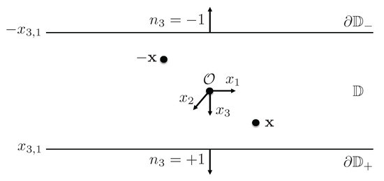
Figure 1. Configuration for the reciprocity theorems.

Consider the quantity ${\partial }_3\left\{{\mathbf{q}}_A^t\left(\mathbf{x}\right)\mathbf{N}{\mathbf{q}}_B\left(\mathbf{x}\right)\right\}$. Applying the product rule for differentiation gives

$$\begin{array}{c}\hfill {\partial }_3\left\{{\mathbf{q}}_A^t\left(\mathbf{x}\right)\mathbf{N}{\mathbf{q}}_B\left(\mathbf{x}\right)\right\}=\left\{{\partial }_3{\mathbf{q}}_A^t\left(\mathbf{x}\right)\right\}\mathbf{N}{\mathbf{q}}_B\left(\mathbf{x}\right)+{\mathbf{q}}_A^t\left(\mathbf{x}\right)\mathbf{N}\left\{{\partial }_3{\mathbf{q}}_B\left(\mathbf{x}\right)\right\}.\end{array}$$

(14)

Integrating both sides over domain $\mathbb{D}$, using the theorem of Gauss on the left-hand side and wave Equation (1) on the right-hand side yields

$$\begin{array}{c}\hfill {\int }_{\partial \mathbb{D}}{\mathbf{q}}_A^t\left(\mathbf{x}\right)\mathbf{N}{\mathbf{q}}_B\left(\mathbf{x}\right)n_3{\mathrm{d}}^2{\mathbf{x}}_{\mathrm{H}}={\int }_{\mathbb{D}}\left[{\{{\mathcal{A}}_A\left(\mathbf{x}\right){\mathbf{q}}_A\left(\mathbf{x}\right)+{\mathbf{d}}_A\left(\mathbf{x}\right)\}}^t\mathbf{N}{\mathbf{q}}_B\left(\mathbf{x}\right)+{\mathbf{q}}_A^t\left(\mathbf{x}\right)\mathbf{N}\{{\mathcal{A}}_B\left(\mathbf{x}\right){\mathbf{q}}_B\left(\mathbf{x}\right)+{\mathbf{d}}_B\left(\mathbf{x}\right)\}\right]{\mathrm{d}}^3\mathbf{x}.\end{array}$$

(15)

Here, ${\mathbf{x}}_{\mathrm{H}}$ is the horizontal coordinate vector $(x_1,x_2)$. Using symmetry relation (7) on the right-hand side and reordering the terms gives

$$\begin{array}{c}\hfill {\int }_{\partial \mathbb{D}}{\mathbf{q}}_A^t\left(\mathbf{x}\right)\mathbf{N}{\mathbf{q}}_B\left(\mathbf{x}\right)n_3{\mathrm{d}}^2{\mathbf{x}}_{\mathrm{H}}={\int }_{\mathbb{D}}\left[{\mathbf{q}}_A^t\left(\mathbf{x}\right)\mathbf{N}\{{\mathcal{A}}_B\left(\mathbf{x}\right)-{\mathcal{A}}_A\left(\mathbf{x}\right)\}{\mathbf{q}}_B\left(\mathbf{x}\right)+{\mathbf{d}}_A^t\left(\mathbf{x}\right)\mathbf{N}{\mathbf{q}}_B\left(\mathbf{x}\right)+{\mathbf{q}}_A^t\left(\mathbf{x}\right)\mathbf{N}{\mathbf{d}}_B\left(\mathbf{x}\right)\right]{\mathrm{d}}^3\mathbf{x}.\end{array}$$

(16)

This is a unified reciprocity theorem of the convolution type (since terms such as ${\mathbf{q}}_A^t\left(\mathbf{x}\right)\mathbf{N}{\mathbf{q}}_B\left(\mathbf{x}\right)$ in the frequency domain correspond to convolutions in the time domain). It does not rely on $\mathcal{PT}$-symmetry.

Next, consider the quantity ${\partial }_3\left\{{\mathbf{q}}_A^{†}(-\mathbf{x})\mathbf{N}{\mathbf{q}}_B\left(\mathbf{x}\right)\right\}$. Following a similar procedure as above, but this time using auxiliary wave Equation (13), we obtain

$$\begin{array}{c}\hfill {\int }_{\partial \mathbb{D}}{\mathbf{q}}_A^{†}(-\mathbf{x})\mathbf{N}{\mathbf{q}}_B\left(\mathbf{x}\right)n_3{\mathrm{d}}^2{\mathbf{x}}_{\mathrm{H}}={\int }_{\mathbb{D}}\left[{\mathbf{q}}_A^{†}(-\mathbf{x})\mathbf{N}\{{\mathcal{A}}_B\left(\mathbf{x}\right)-{\mathcal{A}}_A\left(\mathbf{x}\right)\}{\mathbf{q}}_B\left(\mathbf{x}\right)-{\mathbf{d}}_A^{†}(-\mathbf{x})\mathbf{N}{\mathbf{q}}_B\left(\mathbf{x}\right)+{\mathbf{q}}_A^{†}(-\mathbf{x})\mathbf{N}{\mathbf{d}}_B\left(\mathbf{x}\right)\right]{\mathrm{d}}^3\mathbf{x}.\end{array}$$

(17)

This is a unified reciprocity theorem of the correlation type (since terms such as ${\mathbf{q}}_A^{†}(-\mathbf{x})\mathbf{N}{\mathbf{q}}_B\left(\mathbf{x}\right)$ in the frequency domain correspond to correlations in the time domain). Since we used wave Equation (13) for its derivation, it only holds for $\mathcal{PT}$-symmetric media. Note that the integration boundary on the left-hand side is defined as $\partial \mathbb{D}=\partial {\mathbb{D}}_{-}\cup \partial {\mathbb{D}}_{+}$. For the integration along $\partial {\mathbb{D}}_{-}$, the fields ${\mathbf{q}}_A(-\mathbf{x})$ and ${\mathbf{q}}_B\left(\mathbf{x}\right)$ are evaluated at $\partial {\mathbb{D}}_{+}$ and $\partial {\mathbb{D}}_{-}$, respectively. Similarly, for the integration along $\partial {\mathbb{D}}_{+}$, the fields ${\mathbf{q}}_A(-\mathbf{x})$ and ${\mathbf{q}}_B\left(\mathbf{x}\right)$ are evaluated at $\partial {\mathbb{D}}_{-}$ and $\partial {\mathbb{D}}_{+}$, respectively.

Next, consider the quantity ${\partial }_3\left\{{\mathbf{q}}_A^{†}\left(\mathbf{x}\right)\mathbf{K}{\mathbf{q}}_B\left(\mathbf{x}\right)\right\}$. A similar procedure as above, using wave Equation (1) and symmetry relation (), yields

$$\begin{array}{c}\hfill {\int }_{\partial \mathbb{D}}{\mathbf{q}}_A^{†}\left(\mathbf{x}\right)\mathbf{K}{\mathbf{q}}_B\left(\mathbf{x}\right)n_3{\mathrm{d}}^2{\mathbf{x}}_{\mathrm{H}}={\int }_{\mathbb{D}}\left[{\mathbf{q}}_A^{†}\left(\mathbf{x}\right)\mathbf{K}\{{\mathcal{A}}_B\left(\mathbf{x}\right)-{\overline{\mathcal{A}}}_A\left(\mathbf{x}\right)\}{\mathbf{q}}_B\left(\mathbf{x}\right)+{\mathbf{d}}_A^{†}\left(\mathbf{x}\right)\mathbf{K}{\mathbf{q}}_B\left(\mathbf{x}\right)+{\mathbf{q}}_A^{†}\left(\mathbf{x}\right)\mathbf{K}{\mathbf{d}}_B\left(\mathbf{x}\right)\right]{\mathrm{d}}^3\mathbf{x}.\end{array}$$

(18)

This is a unified reciprocity theorem of the correlation type which does not rely on $\mathcal{PT}$-symmetry.

Finally, consider the quantity ${\partial }_3\left\{{\mathbf{q}}_A^t(-\mathbf{x})\mathbf{K}{\mathbf{q}}_B\left(\mathbf{x}\right)\right\}$. Following the same procedure, using auxiliary wave Equation (13) and symmetry relation (8), yields

$$\begin{array}{c}\hfill {\int }_{\partial \mathbb{D}}{\mathbf{q}}_A^t(-\mathbf{x})\mathbf{K}{\mathbf{q}}_B\left(\mathbf{x}\right)n_3{\mathrm{d}}^2{\mathbf{x}}_{\mathrm{H}}={\int }_{\mathbb{D}}\left[{\mathbf{q}}_A^t(-\mathbf{x})\mathbf{K}\{{\mathcal{A}}_B\left(\mathbf{x}\right)-{\overline{\mathcal{A}}}_A\left(\mathbf{x}\right)\}{\mathbf{q}}_B\left(\mathbf{x}\right)-{\mathbf{d}}_A^t(-\mathbf{x})\mathbf{K}{\mathbf{q}}_B\left(\mathbf{x}\right)+{\mathbf{q}}_A^t(-\mathbf{x})\mathbf{K}{\mathbf{d}}_B\left(\mathbf{x}\right)\right]{\mathrm{d}}^3\mathbf{x}.\end{array}$$

(19)

This is a unified reciprocity theorem of the convolution type which only holds for $\mathcal{PT}$-symmetric media.

Equations (16) and (18) were already known [28,48,49]; they hold for arbitrary inhomogeneous media. Equations (17) and (19) are new; they hold for inhomogeneous media media with $\mathcal{PT}$ symmetry. We will use these reciprocity theorems as a basis to derive unified wave field representations (Section 5), relations between reflection and transmission responses (Section 6), and a Marchenko scheme (Section 7). Before we come to this, we first analyze the boundary integrals in the four reciprocity theorems.

4. Analysis of the Boundary Integrals

From here onward we consider the situation in which the medium (or potential) at and outside $\partial \mathbb{D}$ is homogeneous, lossless, and identical in both half-spaces and in both states. For the analysis of the boundary integrals we define a $N\times 1$ wave-field vector $\mathbf{p}$, according to

$$\begin{array}{c}\hfill \mathbf{p}=\left(\begin{array}{c}{\mathbf{p}}^{+}\\ {\mathbf{p}}^{-}\end{array}\right),\end{array}$$

(20)

where ${\mathbf{p}}^{+}$ and ${\mathbf{p}}^{-}$ are $N/2\times 1$ vectors containing flux-normalised downgoing and upgoing wave fields, respectively (for a comprehensive discussion on flux-normalised versus field-normalised decomposition, see reference [50]). At the boundary $\partial \mathbb{D}$ we relate the wave-field vector $\mathbf{q}$ to $\mathbf{p}$ in states A and B via

$$\begin{array}{ccc}\hfill {\mathbf{q}}_A\left(\mathbf{x}\right)& =& \mathcal{L}\left(\mathbf{x}\right){\mathbf{p}}_A\left(\mathbf{x}\right),\hfill \end{array}$$

(21)

$$\begin{array}{ccc}\hfill {\mathbf{q}}_B\left(\mathbf{x}\right)& =& \mathcal{L}\left(\mathbf{x}\right){\mathbf{p}}_B\left(\mathbf{x}\right),\hfill \end{array}$$

(22)

for $x_3=\pm x_{3,1}$, where $\mathcal{L}\left(\mathbf{x}\right)$ is a $N\times N$ operator matrix, which composes the wave-field vectors ${\mathbf{q}}_{A,B}$ from their downgoing and upgoing constituents ${\mathbf{p}}_{A,B}^{+}$ and ${\mathbf{p}}_{A,B}^{-}$. Note that $\mathcal{L}$ in Equations (21) and (22) is without subscript A or B, since the medium parameters (or potentials) at $\partial \mathbb{D}$ in both states are identical. Explicit expressions for the spatial Fourier transform of $\mathcal{L}$ are given in Appendix A for acoustic, quantum-mechanical, electromagnetic and elastodynamic waves. Substituting Equations (21) and (22) in the boundary integrals of reciprocity theorems (16)–(19), we derive in Appendix B, using specific symmetry properties of $\mathcal{L}$,

$$\begin{array}{ccc}\hfill {\int }_{\partial \mathbb{D}}{\mathbf{q}}_A^t\left(\mathbf{x}\right)\mathbf{N}{\mathbf{q}}_B\left(\mathbf{x}\right)n_3{\mathrm{d}}^2{\mathbf{x}}_{\mathrm{H}}& =& -{\int }_{\partial \mathbb{D}}{\mathbf{p}}_A^t\left(\mathbf{x}\right)\mathbf{N}{\mathbf{p}}_B\left(\mathbf{x}\right)n_3{\mathrm{d}}^2{\mathbf{x}}_{\mathrm{H}},\hfill \end{array}$$

(23)

$$\begin{array}{ccc}\hfill {\int }_{\partial \mathbb{D}}{\mathbf{q}}_A^{†}(-\mathbf{x})\mathbf{N}{\mathbf{q}}_B\left(\mathbf{x}\right)n_3{\mathrm{d}}^2{\mathbf{x}}_{\mathrm{H}}& \approx & -{\int }_{\partial \mathbb{D}}{\mathbf{p}}_A^{†}(-\mathbf{x})\mathbf{N}{\mathbf{p}}_B\left(\mathbf{x}\right)n_3{\mathrm{d}}^2{\mathbf{x}}_{\mathrm{H}},\hfill \end{array}$$

(24)

$$\begin{array}{ccc}\hfill {\int }_{\partial \mathbb{D}}{\mathbf{q}}_A^{†}\left(\mathbf{x}\right)\mathbf{K}{\mathbf{q}}_B\left(\mathbf{x}\right)n_3{\mathrm{d}}^2{\mathbf{x}}_{\mathrm{H}}& \approx & {\int }_{\partial \mathbb{D}}{\mathbf{p}}_A^{†}\left(\mathbf{x}\right)\mathbf{J}{\mathbf{p}}_B\left(\mathbf{x}\right)n_3{\mathrm{d}}^2{\mathbf{x}}_{\mathrm{H}},\hfill \end{array}$$

(25)

$$\begin{array}{ccc}\hfill {\int }_{\partial \mathbb{D}}{\mathbf{q}}_A^t(-\mathbf{x})\mathbf{K}{\mathbf{q}}_B\left(\mathbf{x}\right)n_3{\mathrm{d}}^2{\mathbf{x}}_{\mathrm{H}}& =& {\int }_{\partial \mathbb{D}}{\mathbf{p}}_A^t(-\mathbf{x})\mathbf{J}{\mathbf{p}}_B\left(\mathbf{x}\right)n_3{\mathrm{d}}^2{\mathbf{x}}_{\mathrm{H}}.\hfill \end{array}$$

(26)

Equations (23) and (25) were already known [51]; Equations (24) and (26) are new. The approximation signs in equations (24) and (25) denote that evanescent waves are ignored at $\partial \mathbb{D}$. In the following, we replace ≈ by = when the only approximation is the negligence of evanescent waves.

Using Equations (10) and (20), we can rewrite the right-hand sides of Equations (23)–(26) explicitly in terms of downgoing and upgoing waves at $\partial \mathbb{D}$, according to

$$\begin{array}{ccc}\hfill {\int }_{\partial \mathbb{D}}{\mathbf{q}}_A^t\left(\mathbf{x}\right)\mathbf{N}{\mathbf{q}}_B\left(\mathbf{x}\right)n_3{\mathrm{d}}^2{\mathbf{x}}_{\mathrm{H}}& =& -{\int }_{\partial \mathbb{D}}\left({\left\{{\mathbf{p}}_A^{+}\left(\mathbf{x}\right)\right\}}^t{\mathbf{p}}_B^{-}\left(\mathbf{x}\right)-{\left\{{\mathbf{p}}_A^{-}\left(\mathbf{x}\right)\right\}}^t{\mathbf{p}}_B^{+}\left(\mathbf{x}\right)\right)n_3{\mathrm{d}}^2{\mathbf{x}}_{\mathrm{H}},\hfill \end{array}$$

(27)

$$\begin{array}{ccc}\hfill {\int }_{\partial \mathbb{D}}{\mathbf{q}}_A^{†}(-\mathbf{x})\mathbf{N}{\mathbf{q}}_B\left(\mathbf{x}\right)n_3{\mathrm{d}}^2{\mathbf{x}}_{\mathrm{H}}& =& -{\int }_{\partial \mathbb{D}}\left({\left\{{\mathbf{p}}_A^{+}(-\mathbf{x})\right\}}^{†}{\mathbf{p}}_B^{-}\left(\mathbf{x}\right)-{\left\{{\mathbf{p}}_A^{-}(-\mathbf{x})\right\}}^{†}{\mathbf{p}}_B^{+}\left(\mathbf{x}\right)\right)n_3{\mathrm{d}}^2{\mathbf{x}}_{\mathrm{H}},\hfill \end{array}$$

(28)

$$\begin{array}{ccc}\hfill {\int }_{\partial \mathbb{D}}{\mathbf{q}}_A^{†}\left(\mathbf{x}\right)\mathbf{K}{\mathbf{q}}_B\left(\mathbf{x}\right)n_3{\mathrm{d}}^2{\mathbf{x}}_{\mathrm{H}}& =& {\int }_{\partial \mathbb{D}}\left({\left\{{\mathbf{p}}_A^{+}\left(\mathbf{x}\right)\right\}}^{†}{\mathbf{p}}_B^{+}\left(\mathbf{x}\right)-{\left\{{\mathbf{p}}_A^{-}\left(\mathbf{x}\right)\right\}}^{†}{\mathbf{p}}_B^{-}\left(\mathbf{x}\right)\right)n_3{\mathrm{d}}^2{\mathbf{x}}_{\mathrm{H}},\hfill \end{array}$$

(29)

$$\begin{array}{ccc}\hfill {\int }_{\partial \mathbb{D}}{\mathbf{q}}_A^t(-\mathbf{x})\mathbf{K}{\mathbf{q}}_B\left(\mathbf{x}\right)n_3{\mathrm{d}}^2{\mathbf{x}}_{\mathrm{H}}& =& {\int }_{\partial \mathbb{D}}\left({\left\{{\mathbf{p}}_A^{+}(-\mathbf{x})\right\}}^t{\mathbf{p}}_B^{+}\left(\mathbf{x}\right)-{\left\{{\mathbf{p}}_A^{-}(-\mathbf{x})\right\}}^t{\mathbf{p}}_B^{-}\left(\mathbf{x}\right)\right)n_3{\mathrm{d}}^2{\mathbf{x}}_{\mathrm{H}}.\hfill \end{array}$$

(30)

These equations will be used in Section 6 for the derivation of relations between reflection and transmission responses. Here we consider a special case. Let us assume that the medium outside $\mathbb{D}$ is source free and that the wave fields in both states are responses to sources in $\mathbb{D}$. This implies that at $\partial \mathbb{D}$ all waves are outward propagating, i.e., at $\partial {\mathbb{D}}_{-}$ there are only upgoing waves and at $\partial {\mathbb{D}}_{+}$ only downgoing waves. Hence, ${\mathbf{p}}_A^{+}\left(\mathbf{x}\right)={\mathbf{p}}_B^{+}\left(\mathbf{x}\right)={\mathbf{p}}_A^{-}(-\mathbf{x})={\mathbf{p}}_B^{-}(-\mathbf{x})=\mathbf{0}$ for $\mathbf{x}$ at $\partial {\mathbb{D}}_{-}$ and ${\mathbf{p}}_A^{+}(-\mathbf{x})={\mathbf{p}}_B^{+}(-\mathbf{x})={\mathbf{p}}_A^{-}\left(\mathbf{x}\right)={\mathbf{p}}_B^{-}\left(\mathbf{x}\right)=\mathbf{0}$ for $\mathbf{x}$ at $\partial {\mathbb{D}}_{+}$ (here $\mathbf{0}$ is a $N/2\times 1$ zero vector). Using this in Equations (30) and (27) yields

$$\begin{array}{ccc}\hfill {\int }_{\partial \mathbb{D}}{\mathbf{q}}_A^t\left(\mathbf{x}\right)\mathbf{N}{\mathbf{q}}_B\left(\mathbf{x}\right)n_3{\mathrm{d}}^2{\mathbf{x}}_{\mathrm{H}}& =& 0,\hfill \end{array}$$

(31)

$$\begin{array}{ccc}\hfill {\int }_{\partial \mathbb{D}}{\mathbf{q}}_A^t(-\mathbf{x})\mathbf{K}{\mathbf{q}}_B\left(\mathbf{x}\right)n_3{\mathrm{d}}^2{\mathbf{x}}_{\mathrm{H}}& =& 0.\hfill \end{array}$$

(32)

Equation (31) is a compact form of the well-known Sommerfeld radiation condition; Equation (32) is a new radiation condition.

5. Wave Field Representations

We use the reciprocity theorems derived in Section 3 as the basis for deriving wave field representations. In Section 5.1 we discuss the unified Green’s matrix and its symmetry properties. In Section 5.2 we derive a wave field representation by choosing Green’s state for state A. In Section 5.3 we derive representations for back-propagation and for Green’s matrix retrieval, also known as interferometry. We consider arbitrary inhomogeneous media and media with $\mathcal{PT}$-symmetry in $\mathbb{D}$, embedded between two identical homogeneous lossless half-spaces.

5.1. Green’s Matrix and Its Symmetry Properties

We introduce the $N\times N$ Green’s matrix $\mathbf{G}(\mathbf{x},{\mathbf{x}}_A)$ for an arbitrary inhomogeneous medium in $\mathbb{D}$ as the solution of

$$\begin{array}{c}\hfill {\partial }_3\mathbf{G}-\mathcal{A}\mathbf{G}=\mathbf{I}\delta (\mathbf{x}-{\mathbf{x}}_A),\end{array}$$

(33)

where $\delta \left(\mathbf{x}\right)$ is a Dirac delta distribution, and ${\mathbf{x}}_A=(x_{1,A},x_{2,A},x_{3,A})$ defines the position of a unit point source. We further demand that the time-domain Green’s matrix $\mathbf{G}(\mathbf{x},{\mathbf{x}}_A,t)$ is causal, hence $\mathbf{G}(\mathbf{x},{\mathbf{x}}_A,t<0)=\mathbf{O}$. Similar to operator matrix $\mathcal{A}$, Green’s matrix is partitioned as

$$\begin{array}{c}\hfill \mathbf{G}(\mathbf{x},{\mathbf{x}}_A)=\left(\begin{array}{cc}{\mathbf{G}}_{11}& {\mathbf{G}}_{12}\\ {\mathbf{G}}_{21}& {\mathbf{G}}_{22}\end{array}\right)(\mathbf{x},{\mathbf{x}}_A).\end{array}$$

(34)

We derive a symmetry property of Green’s matrix. We replace ${\mathbf{q}}_A$ and ${\mathbf{q}}_B$ in reciprocity theorem (16) by Green’s matrices $\mathbf{G}(\mathbf{x},{\mathbf{x}}_A)$ and $\mathbf{G}(\mathbf{x},{\mathbf{x}}_B)$, respectively. Similarly, we replace the source vectors ${\mathbf{d}}_A$ and ${\mathbf{d}}_B$ by $\mathbf{I}\delta (\mathbf{x}-{\mathbf{x}}_A)$ and $\mathbf{I}\delta (\mathbf{x}-{\mathbf{x}}_B)$, respectively, with ${\mathbf{x}}_A$ and ${\mathbf{x}}_B$ denoting the source positions, both in $\mathbb{D}$. Both Green’s matrices are defined in the same medium; hence, ${\mathcal{A}}_A={\mathcal{A}}_B=\mathcal{A}$. This implies that the first term under the integral on the right-hand side of Equation (16) vanishes. Since the medium outside $\mathbb{D}$ is homogeneous, Green’s matrices at $\partial \mathbb{D}$ are outward propagating. This implies that the integral on the left-hand side of Equation (16) also vanishes, see Equation (31). From the remaining integral, we thus obtain the following symmetry property of Green’s matrix

$$\begin{array}{c}\hfill {\mathbf{G}}^t({\mathbf{x}}_B,{\mathbf{x}}_A)\mathbf{N}=-\mathbf{N}\mathbf{G}({\mathbf{x}}_A,{\mathbf{x}}_B).\end{array}$$

(35)

This is the well-known source-receiver reciprocity relation, which holds for arbitrary inhomogeneous media in $\mathbb{D}$. It is illustrated in Figure 2a. Next, we define $\overline{\mathbf{G}}(\mathbf{x},{\mathbf{x}}_A)$ as the outward propagating Green’s matrix of the adjoint medium, obeying the following wave equation

$$\begin{array}{c}\hfill {\partial }_3\overline{\mathbf{G}}-\overline{\mathcal{A}}\overline{\mathbf{G}}=\mathbf{I}\delta (\mathbf{x}-{\mathbf{x}}_A).\end{array}$$

(36)

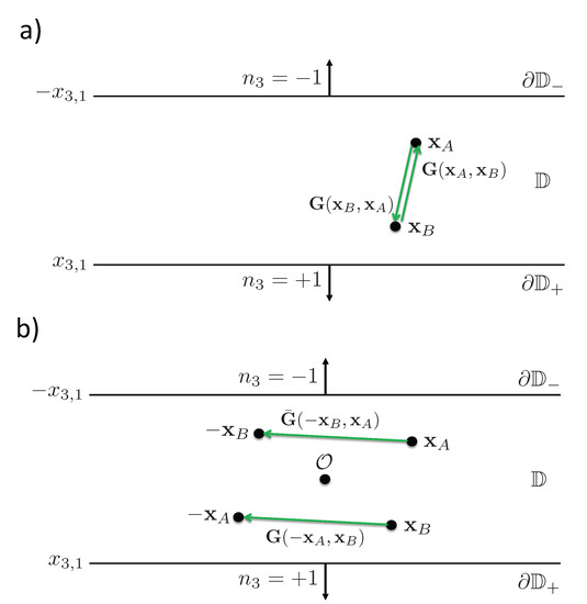
Figure 2. (a) Source-receiver reciprocity for an arbitrary inhomogeneous medium in $\mathbb{D}$ (Equations (35) and (40)). (b) Additional source-receiver reciprocity for a medium with $\mathcal{PT}$-symmetry in $\mathbb{D}$ (Equations (41) and (42)). The rays in these and subsequent figures represent full multi-component responses (direct waves, (multiply-)scattered waves, converted waves etc.) between the source and receiver points.

We will combine $\mathbf{G}(\mathbf{x},{\mathbf{x}}_A)$ and the complex conjugate of $\overline{\mathbf{G}}(\mathbf{x},{\mathbf{x}}_A)$ to form a so-called homogeneous Green’s matrix, i.e., a Green’s matrix obeying a wave equation without a source term on the right-hand side. To this end, we first pre-and post-multiply all terms in Equation (36) by $\mathbf{J}$, use Equation (6) and $\mathbf{J}\mathbf{J}=\mathbf{I}$ and subsequently take the complex conjugate of all terms. This yields

$$\begin{array}{c}\hfill {\partial }_3\mathbf{J}{\overline{\mathbf{G}}}^{*}\mathbf{J}-\mathcal{A}\mathbf{J}{\overline{\mathbf{G}}}^{*}\mathbf{J}=\mathbf{I}\delta (\mathbf{x}-{\mathbf{x}}_A).\end{array}$$

(37)

Subtracting all terms of this equation from the corresponding terms in Equation (33) yields

$$\begin{array}{c}\hfill {\partial }_3{\mathbf{G}}_{\mathrm{h}}-\mathcal{A}{\mathbf{G}}_{\mathrm{h}}=\mathbf{O}\end{array}$$

(38)

with the homogeneous Green’s matrix ${\mathbf{G}}_{\mathrm{h}}(\mathbf{x},{\mathbf{x}}_A)$ defined as

$$\begin{array}{c}\hfill {\mathbf{G}}_{\mathrm{h}}(\mathbf{x},{\mathbf{x}}_A)=\mathbf{G}(\mathbf{x},{\mathbf{x}}_A)-\mathbf{J}{\overline{\mathbf{G}}}^{*}(\mathbf{x},{\mathbf{x}}_A)\mathbf{J}.\end{array}$$

(39)

Using symmetry relation (35), $\mathbf{J}\mathbf{N}=-\mathbf{N}\mathbf{J}$ and ${\mathbf{J}}^t=\mathbf{J}$, we find the following reciprocity relation for the homogeneous Green’s matrix

$$\begin{array}{c}\hfill {\mathbf{G}}_{\mathrm{h}}^t({\mathbf{x}}_B,{\mathbf{x}}_A)\mathbf{N}=-\mathbf{N}{\mathbf{G}}_{\mathrm{h}}({\mathbf{x}}_A,{\mathbf{x}}_B).\end{array}$$

(40)

Next, we derive symmetry properties of Green’s matrix and the homogeneous Green’s matrix for $\mathcal{PT}$-symmetric media in $\mathbb{D}$. We replace ${\mathbf{q}}_A$ and ${\mathbf{q}}_B$ in reciprocity theorem (19) by Green’s matrices $\overline{\mathbf{G}}(\mathbf{x},{\mathbf{x}}_A)$ and $\mathbf{G}(\mathbf{x},{\mathbf{x}}_B)$, respectively. Since ${\mathcal{A}}_A=\overline{\mathcal{A}}$ (see Equation (36)) and ${\mathcal{A}}_B=\mathcal{A}$ (as before) we have ${\overline{\mathcal{A}}}_A={\mathcal{A}}_B$, hence, the first term under the integral on the right-hand side of Equation (19) vanishes. Since the medium outside $\mathbb{D}$ is homogeneous, the integral on the left-hand side of Equation (19) also vanishes, see Equation (32). From the remaining integral, we thus obtain the following symmetry property of Green’s matrix

$$\begin{array}{c}\hfill {\overline{\mathbf{G}}}^t(-{\mathbf{x}}_B,{\mathbf{x}}_A)\mathbf{K}=\mathbf{K}\mathbf{G}(-{\mathbf{x}}_A,{\mathbf{x}}_B).\end{array}$$

(41)

This is an additional source-receiver reciprocity relation, which only holds for media with $\mathcal{PT}$-symmetry. It is illustrated in Figure 2b. Using symmetry relation (41), $\mathbf{J}\mathbf{K}=-\mathbf{K}\mathbf{J}$ and ${\mathbf{J}}^t=\mathbf{J}$, we find the following reciprocity relation for the homogeneous Green’s matrix in $\mathcal{PT}$-symmetric media

$$\begin{array}{c}\hfill {\overline{\mathbf{G}}}_{\mathrm{h}}^t(-{\mathbf{x}}_B,{\mathbf{x}}_A)\mathbf{K}=\mathbf{K}{\mathbf{G}}_{\mathrm{h}}(-{\mathbf{x}}_A,{\mathbf{x}}_B).\end{array}$$

(42)

5.2. Wave Field Representation

We derive a general wave field representation from the reciprocity theorem of the convolution type for arbitrary inhomogeneous media (Equation (16)). For state A we choose Green’s state; hence, we replace ${\mathbf{q}}_A$ and ${\mathbf{d}}_A$ by Green’s matrix $\mathbf{G}(\mathbf{x},{\mathbf{x}}_A)$ and unit source matrix $\mathbf{I}\delta (\mathbf{x}-{\mathbf{x}}_A)$, with ${\mathbf{x}}_A$ in $\mathbb{D}$; we leave operator ${\mathcal{A}}_A$ as is. For state B we choose the actual wave state. To this end we drop the subscripts B from ${\mathbf{q}}_B$, ${\mathbf{d}}_B$ and ${\mathcal{A}}_B$. We thus obtain from Equation (16)

$$\begin{array}{c}\hfill \mathbf{N}\mathbf{q}\left({\mathbf{x}}_A\right)=-{\int }_{\mathbb{D}}{\mathbf{G}}^t(\mathbf{x},{\mathbf{x}}_A)\mathbf{N}\mathbf{d}\left(\mathbf{x}\right){\mathrm{d}}^3\mathbf{x}+{\int }_{\partial \mathbb{D}}{\mathbf{G}}^t(\mathbf{x},{\mathbf{x}}_A)\mathbf{N}\mathbf{q}\left(\mathbf{x}\right)n_3{\mathrm{d}}^2{\mathbf{x}}_{\mathrm{H}}-{\int }_{\mathbb{D}}{\mathbf{G}}^t(\mathbf{x},{\mathbf{x}}_A)\mathbf{N}\{\mathcal{A}-{\mathcal{A}}_A\}\mathbf{q}\left(\mathbf{x}\right){\mathrm{d}}^3\mathbf{x}.\end{array}$$

(43)

Using the symmetry property of Green’s matrix, formulated by Equation (35), we obtain

$$\begin{array}{c}\hfill \mathbf{q}\left({\mathbf{x}}_A\right)={\int }_{\mathbb{D}}\mathbf{G}({\mathbf{x}}_A,\mathbf{x})\mathbf{d}\left(\mathbf{x}\right){\mathrm{d}}^3\mathbf{x}-{\int }_{\partial \mathbb{D}}\mathbf{G}({\mathbf{x}}_A,\mathbf{x})\mathbf{q}\left(\mathbf{x}\right)n_3{\mathrm{d}}^2{\mathbf{x}}_{\mathrm{H}}+{\int }_{\mathbb{D}}\mathbf{G}({\mathbf{x}}_A,\mathbf{x})\{\mathcal{A}-{\mathcal{A}}_A\}\mathbf{q}\left(\mathbf{x}\right){\mathrm{d}}^3\mathbf{x}.\end{array}$$

(44)

This is the unified wave field representation of the convolution type, which does not rely on $\mathcal{PT}$-symmetry. The left-hand side is the wave field vector $\mathbf{q}\left({\mathbf{x}}_A\right)$ at a specific position ${\mathbf{x}}_A$. It is expressed in terms of a volume integral containing the source distribution $\mathbf{d}\left(\mathbf{x}\right)$ in $\mathbb{D}$, a unified Kirchhoff–Helmholtz boundary integral and an integral containing the contrast operator $\mathcal{A}-{\mathcal{A}}_A$ in $\mathbb{D}$. It finds applications in forward modelling [48,49,52], of which a further discussion is beyond the scope of this paper.

5.3. Back-Propagation and Interferometric Green’s Matrix Retrieval

We derive representations for back-propagation and for interferometric Green’s matrix retrieval from the reciprocity theorem of the correlation type for arbitrary inhomogeneous media (Equation (18)). We replace the wave-field vectors ${\mathbf{q}}_A$ and ${\mathbf{q}}_B$ by Green’s matrices $\overline{\mathbf{G}}(\mathbf{x},{\mathbf{x}}_A)$ and $\mathbf{G}(\mathbf{x},{\mathbf{x}}_B)$, respectively. Accordingly, the source vectors ${\mathbf{d}}_A$ and ${\mathbf{d}}_B$ are replaced by source matrices $\mathbf{I}\delta (\mathbf{x}-{\mathbf{x}}_A)$ and $\mathbf{I}\delta (\mathbf{x}-{\mathbf{x}}_B)$, with ${\mathbf{x}}_A$ and ${\mathbf{x}}_B$ both in $\mathbb{D}$. For the operator matrices we choose ${\mathcal{A}}_A=\overline{\mathcal{A}}$ (since Green’s matrix in state A is defined in the adjoint medium) and ${\mathcal{A}}_B=\mathcal{A}$. These choices imply that the first term under the integral on the right-hand side of Equation (18) vanishes. From the remaining terms in this equation we obtain

$$\begin{array}{c}\hfill \mathbf{K}\mathbf{G}({\mathbf{x}}_A,{\mathbf{x}}_B)+{\overline{\mathbf{G}}}^{†}({\mathbf{x}}_B,{\mathbf{x}}_A)\mathbf{K}={\int }_{\partial \mathbb{D}}{\overline{\mathbf{G}}}^{†}(\mathbf{x},{\mathbf{x}}_A)\mathbf{K}\mathbf{G}(\mathbf{x},{\mathbf{x}}_B)n_3{\mathrm{d}}^2{\mathbf{x}}_{\mathrm{H}}.\end{array}$$

(45)

Using $\mathbf{K}=-\mathbf{N}\mathbf{J}$, the symmetry property of Green’s matrix formulated by Equation (35) and $\mathbf{N}=-\mathbf{K}\mathbf{J}$, we rewrite the second term on the left-hand side as $-\mathbf{K}\mathbf{J}{\overline{\mathbf{G}}}^{*}({\mathbf{x}}_A,{\mathbf{x}}_B)\mathbf{J}$. Pre-multiplying both sides of the resulting equation by ${\mathbf{K}}^{-1}$ and using ${\mathbf{K}}^{-1}=\mathbf{K}$, we thus obtain

$$\begin{array}{c}\hfill {\mathbf{G}}_{\mathrm{h}}({\mathbf{x}}_A,{\mathbf{x}}_B)={\int }_{\partial \mathbb{D}}\mathbf{K}{\overline{\mathbf{G}}}^{†}(\mathbf{x},{\mathbf{x}}_A)\mathbf{K}\mathbf{G}(\mathbf{x},{\mathbf{x}}_B)n_3{\mathrm{d}}^2{\mathbf{x}}_{\mathrm{H}},\end{array}$$

(46)

with the homogeneous Green’s matrix ${\mathbf{G}}_{\mathrm{h}}({\mathbf{x}}_A,{\mathbf{x}}_B)$ defined in Equation (39). Equation (46) is a unified form of the classical homogeneous Green’s function representation [53,54]; it does not rely on $\mathcal{PT}$-symmetry. Equation (46) is illustrated in Figure 3a. We can interpret $\mathbf{G}(\mathbf{x},{\mathbf{x}}_B)$ as the response to a source at ${\mathbf{x}}_B$ inside $\mathbb{D}$, observed by receivers at $\mathbf{x}$ at the boundary $\partial \mathbb{D}$, which consists of two planar boundaries $\partial {\mathbb{D}}_{-}$ and $\partial {\mathbb{D}}_{+}$. Green’s matrix ${\overline{\mathbf{G}}}^{†}(\mathbf{x},{\mathbf{x}}_A)$ propagates this response back from $\mathbf{x}$ at the boundary to ${\mathbf{x}}_A$ inside $\mathbb{D}$. The result is the homogeneous Green’s matrix between ${\mathbf{x}}_B$ and ${\mathbf{x}}_A$ (the red arrow in Figure 3a). When these two points coincide, then ${\mathbf{G}}_{\mathrm{h}}({\mathbf{x}}_B,{\mathbf{x}}_B)$ can be interpreted as an image of the source at ${\mathbf{x}}_B$, obtained from observations at $\partial \mathbb{D}$. Equation (46) finds applications in (generalized forms of) inverse source problems [46,55], inverse scattering [12,54,56,57], (holographic) imaging [53,58,59,60,61,62], time-reversal acoustics [63] and interferometric Green’s matrix retrieval from passive measurements [64,65,66]. To explain the latter type of application, we transpose both sides of Equation (46), use Equations (35) and (40), $\mathbf{K}={\mathbf{K}}^t$, ${\mathbf{N}}^{-1}=-\mathbf{N}$ and $\mathbf{N}\mathbf{K}=-\mathbf{K}\mathbf{N}$, to obtain

$$\begin{array}{c}\hfill {\mathbf{G}}_{\mathrm{h}}({\mathbf{x}}_B,{\mathbf{x}}_A)=-{\int }_{\partial \mathbb{D}}\mathbf{G}({\mathbf{x}}_B,\mathbf{x})\mathbf{K}{\overline{\mathbf{G}}}^{†}({\mathbf{x}}_A,\mathbf{x})\mathbf{K}{n}_3{\mathrm{d}}^2{\mathbf{x}}_{\mathrm{H}}.\end{array}$$

(47)

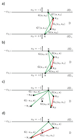
Figure 3. (a) Back propagation in an arbitrary inhomogeneous medium in $\mathbb{D}$ (Equation (46)). (b) Interferometric Green’s matrix retrieval in an arbitrary inhomogeneous medium in $\mathbb{D}$ (Equation (47)). (c) Green’s matrix retrieval in a medium with $\mathcal{PT}$-symmetry in $\mathbb{D}$ (Equation (50)). The integral is single-sided, but four receivers are required in the medium and its adjoint. (d) As in (c), but requiring two receivers only in one-and-the-same lossless medium (Equation (51)).

When the medium is lossless, $\overline{\mathbf{G}}({\mathbf{x}}_A,\mathbf{x})$ and $\mathbf{G}({\mathbf{x}}_B,\mathbf{x})$ can be interpreted as responses to sources at $\mathbf{x}$ at the boundary $\partial \mathbb{D}$, observed by receivers at ${\mathbf{x}}_A$ and ${\mathbf{x}}_B$ inside $\mathbb{D}$ (Figure 3b). The right-hand side of Equation (47) can be seen as (the Fourier transform of) the cross-correlation of these responses, integrated along the boundary $\partial \mathbb{D}$. The left-hand side is the retrieved homogeneous Green’s matrix between ${\mathbf{x}}_A$ and ${\mathbf{x}}_B$. Hence, the receiver at ${\mathbf{x}}_A$ (on the right-hand side of this equation) is turned into a virtual source at ${\mathbf{x}}_A$ (on the left-hand side). When the sources at $\partial \mathbb{D}$ are uncorrelated noise sources, the right-hand side of Equation (47) can be turned into a direct cross-correlation of the noise responses at ${\mathbf{x}}_A$ and ${\mathbf{x}}_B$, without needing an integral along the sources (similar as in references [64,65,66,67,68]; a further discussion of Green’s matrix retrieval from ambient noise is beyond the scope of this paper).

Note that in Equations (46) and (47), the integration boundary $\partial \mathbb{D}$ consists of two boundaries, which together enclose ${\mathbf{x}}_A$ and ${\mathbf{x}}_B$. Hence, depending on the application, one needs either receivers (Equation (46)) or sources (Equation (47)) on both boundaries $\partial {\mathbb{D}}_{-}$ and $\partial {\mathbb{D}}_{+}$. In many practical situations, a medium is accessible from one side only, meaning that the integral can only be evaluated along a single boundary. For media with $\mathcal{PT}$-symmetry, the integral along the two-sided boundary $\partial \mathbb{D}$ can be turned into an integral along only one of the boundaries $\partial {\mathbb{D}}_{-}$ or $\partial {\mathbb{D}}_{+}$. We illustrate this for Equation (47). Using that $n_3=\pm 1$ at $\partial {\mathbb{D}}_{\pm }$, Equation (47) can be rewritten as

$$\begin{array}{c}\hfill {\mathbf{G}}_{\mathrm{h}}({\mathbf{x}}_B,{\mathbf{x}}_A)={\int }_{\partial {\mathbb{D}}_{-}}\mathbf{G}({\mathbf{x}}_B,\mathbf{x})\mathbf{K}{\overline{\mathbf{G}}}^{†}({\mathbf{x}}_A,\mathbf{x})\mathbf{K}{\mathrm{d}}^2{\mathbf{x}}_{\mathrm{H}}-{\int }_{\partial {\mathbb{D}}_{+}}\mathbf{G}({\mathbf{x}}_B,\mathbf{x})\mathbf{K}{\overline{\mathbf{G}}}^{†}({\mathbf{x}}_A,\mathbf{x})\mathbf{K}{\mathrm{d}}^2{\mathbf{x}}_{\mathrm{H}}.\end{array}$$

(48)

For a $\mathcal{PT}$-symmetric medium we can use symmetry relations (35) and (41). Together with the aforementioned properties of $\mathbf{K}$ and $\mathbf{N}$ and $\mathbf{K}\mathbf{N}=-\mathbf{J}$, we thus rewrite the integral along $\partial {\mathbb{D}}_{+}$ as

$$\begin{array}{ccc}\hfill {\int }_{\partial {\mathbb{D}}_{+}}\mathbf{G}({\mathbf{x}}_B,\mathbf{x})\mathbf{K}{\overline{\mathbf{G}}}^{†}({\mathbf{x}}_A,\mathbf{x})\mathbf{K}{\mathrm{d}}^2{\mathbf{x}}_{\mathrm{H}}& =& -{\int }_{\partial {\mathbb{D}}_{+}}\mathbf{J}\overline{\mathbf{G}}(-{\mathbf{x}}_B,-\mathbf{x})\mathbf{K}{\mathbf{G}}^{†}(-{\mathbf{x}}_A,-\mathbf{x})\mathbf{N}{\mathrm{d}}^2{\mathbf{x}}_{\mathrm{H}}\hfill \\ & =& {\int }_{\partial {\mathbb{D}}_{-}}\mathbf{J}\overline{\mathbf{G}}(-{\mathbf{x}}_B,\mathbf{x})\mathbf{K}{\mathbf{G}}^{†}(-{\mathbf{x}}_A,\mathbf{x})\mathbf{N}{\mathrm{d}}^2{\mathbf{x}}_{\mathrm{H}}.\hfill \end{array}$$

(49)

With this, Equation (48) is turned into a single-sided integral, according to

$$\begin{array}{c}\hfill {\mathbf{G}}_{\mathrm{h}}({\mathbf{x}}_B,{\mathbf{x}}_A)={\int }_{\partial {\mathbb{D}}_{-}}\left(\mathbf{G}({\mathbf{x}}_B,\mathbf{x})\mathbf{K}{\overline{\mathbf{G}}}^{†}({\mathbf{x}}_A,\mathbf{x})\mathbf{K}-\mathbf{J}\overline{\mathbf{G}}(-{\mathbf{x}}_B,\mathbf{x})\mathbf{K}{\mathbf{G}}^{†}(-{\mathbf{x}}_A,\mathbf{x})\mathbf{N}\right){\mathrm{d}}^2{\mathbf{x}}_{\mathrm{H}}.\end{array}$$

(50)

The evaluation of this integral requires observations at four positions in the $\mathcal{PT}$-symmetric medium and its adjoint (Figure 3c). For the special case that ${\mathbf{x}}_B=-{\mathbf{x}}_A$ and the medium is lossless, we obtain

$$\begin{array}{c}\hfill {\mathbf{G}}_{\mathrm{h}}(-{\mathbf{x}}_A,{\mathbf{x}}_A)={\int }_{\partial {\mathbb{D}}_{-}}\left(\mathbf{G}(-{\mathbf{x}}_A,\mathbf{x})\mathbf{K}{\mathbf{G}}^{†}({\mathbf{x}}_A,\mathbf{x})\mathbf{K}-\mathbf{J}\mathbf{G}({\mathbf{x}}_A,\mathbf{x})\mathbf{K}{\mathbf{G}}^{†}(-{\mathbf{x}}_A,\mathbf{x})\mathbf{N}\right){\mathrm{d}}^2{\mathbf{x}}_{\mathrm{H}}.\end{array}$$

(51)

This integral can be evaluated when observations at only two positions are available (Figure 3d).

6. Relations between Reflection and Transmission Responses

In reference [33] we presented a systematic analysis of the relations between reflection and transmission responses of arbitrary inhomogeneous media. Here we extend this analysis for $\mathcal{PT}$-symmetric media.

Consider the configuration of Figure 1, with $\mathbb{D}$ embedded between two identical homogeneous lossless half-spaces. Sources may be present outside $\partial \mathbb{D}$, but we assume there are no sources in $\mathbb{D}$. When the medium in state A is the same as that in state B, we find for this situation from reciprocity theorems (16) and (17)

$$\begin{array}{c}\hfill {\int }_{\partial \mathbb{D}}{\mathbf{q}}_A^t\left(\mathbf{x}\right)\mathbf{N}{\mathbf{q}}_B\left(\mathbf{x}\right)n_3{\mathrm{d}}^2{\mathbf{x}}_{\mathrm{H}}=0\end{array}$$

(52)

and, assuming $\mathcal{PT}$-symmetry,

$$\begin{array}{c}\hfill {\int }_{\partial \mathbb{D}}{\mathbf{q}}_A^{†}(-\mathbf{x})\mathbf{N}{\mathbf{q}}_B\left(\mathbf{x}\right)n_3{\mathrm{d}}^2{\mathbf{x}}_{\mathrm{H}}=0,\end{array}$$

(53)

respectively. On the other hand, when the medium in state A is the adjoint of that in state B, we find from reciprocity theorems (18) and (19)

$$\begin{array}{c}\hfill {\int }_{\partial \mathbb{D}}{\mathbf{q}}_A^{†}\left(\mathbf{x}\right)\mathbf{K}{\mathbf{q}}_B\left(\mathbf{x}\right)n_3{\mathrm{d}}^2{\mathbf{x}}_{\mathrm{H}}=0\end{array}$$

(54)

and, assuming $\mathcal{PT}$-symmetry,

$$\begin{array}{c}\hfill {\int }_{\partial \mathbb{D}}{\mathbf{q}}_A^t(-\mathbf{x})\mathbf{K}{\mathbf{q}}_B\left(\mathbf{x}\right)n_3{\mathrm{d}}^2{\mathbf{x}}_{\mathrm{H}}=0,\end{array}$$

(55)

respectively. Using this for the left-hand sides of Equations (27)–(30), we find that the right-hand sides of those equations are also equal to zero. Dividing $\partial \mathbb{D}$ again into $\partial {\mathbb{D}}_{-}$ and $\partial {\mathbb{D}}_{+}$, with $n_3=-1$ and $n_3=+1$, respectively, we thus obtain

$$\begin{array}{ccc}\hfill {\int }_{\partial {\mathbb{D}}_{-}}\left({\left\{{\mathbf{p}}_A^{+}\left(\mathbf{x}\right)\right\}}^t{\mathbf{p}}_B^{-}\left(\mathbf{x}\right)-{\left\{{\mathbf{p}}_A^{-}\left(\mathbf{x}\right)\right\}}^t{\mathbf{p}}_B^{+}\left(\mathbf{x}\right)\right){\mathrm{d}}^2{\mathbf{x}}_{\mathrm{H}}& =& {\int }_{\partial {\mathbb{D}}_{+}}\left({\left\{{\mathbf{p}}_A^{+}\left(\mathbf{x}\right)\right\}}^t{\mathbf{p}}_B^{-}\left(\mathbf{x}\right)-{\left\{{\mathbf{p}}_A^{-}\left(\mathbf{x}\right)\right\}}^t{\mathbf{p}}_B^{+}\left(\mathbf{x}\right)\right){\mathrm{d}}^2{\mathbf{x}}_{\mathrm{H}},\hfill \end{array}$$

(56)

$$\begin{array}{ccc}\hfill {\int }_{\partial {\mathbb{D}}_{-}}\left({\left\{{\mathbf{p}}_A^{+}(-\mathbf{x})\right\}}^{†}{\mathbf{p}}_B^{-}\left(\mathbf{x}\right)-{\left\{{\mathbf{p}}_A^{-}(-\mathbf{x})\right\}}^{†}{\mathbf{p}}_B^{+}\left(\mathbf{x}\right)\right){\mathrm{d}}^2{\mathbf{x}}_{\mathrm{H}}& =& {\int }_{\partial {\mathbb{D}}_{+}}\left({\left\{{\mathbf{p}}_A^{+}(-\mathbf{x})\right\}}^{†}{\mathbf{p}}_B^{-}\left(\mathbf{x}\right)-{\left\{{\mathbf{p}}_A^{-}(-\mathbf{x})\right\}}^{†}{\mathbf{p}}_B^{+}\left(\mathbf{x}\right)\right){\mathrm{d}}^2{\mathbf{x}}_{\mathrm{H}},\hfill \end{array}$$

(57)

$$\begin{array}{ccc}\hfill {\int }_{\partial {\mathbb{D}}_{-}}\left({\left\{{\mathbf{p}}_A^{+}\left(\mathbf{x}\right)\right\}}^{†}{\mathbf{p}}_B^{+}\left(\mathbf{x}\right)-{\left\{{\mathbf{p}}_A^{-}\left(\mathbf{x}\right)\right\}}^{†}{\mathbf{p}}_B^{-}\left(\mathbf{x}\right)\right){\mathrm{d}}^2{\mathbf{x}}_{\mathrm{H}}& =& {\int }_{\partial {\mathbb{D}}_{+}}\left({\left\{{\mathbf{p}}_A^{+}\left(\mathbf{x}\right)\right\}}^{†}{\mathbf{p}}_B^{+}\left(\mathbf{x}\right)-{\left\{{\mathbf{p}}_A^{-}\left(\mathbf{x}\right)\right\}}^{†}{\mathbf{p}}_B^{-}\left(\mathbf{x}\right)\right){\mathrm{d}}^2{\mathbf{x}}_{\mathrm{H}},\hfill \end{array}$$

(58)

$$\begin{array}{ccc}\hfill {\int }_{\partial {\mathbb{D}}_{-}}\left({\left\{{\mathbf{p}}_A^{+}(-\mathbf{x})\right\}}^t{\mathbf{p}}_B^{+}\left(\mathbf{x}\right)-{\left\{{\mathbf{p}}_A^{-}(-\mathbf{x})\right\}}^t{\mathbf{p}}_B^{-}\left(\mathbf{x}\right)\right){\mathrm{d}}^2{\mathbf{x}}_{\mathrm{H}}& =& {\int }_{\partial {\mathbb{D}}_{+}}\left({\left\{{\mathbf{p}}_A^{+}(-\mathbf{x})\right\}}^t{\mathbf{p}}_B^{+}\left(\mathbf{x}\right)-{\left\{{\mathbf{p}}_A^{-}(-\mathbf{x})\right\}}^t{\mathbf{p}}_B^{-}\left(\mathbf{x}\right)\right){\mathrm{d}}^2{\mathbf{x}}_{\mathrm{H}}.\hfill \end{array}$$

(59)

Equations (56) and (58) hold for arbitrary inhomogeneous media in $\mathbb{D}$, whereas $\mathcal{PT}$-symmetry is assumed for Equations (57) and (59). Equations (56) and (57) hold when the medium in state A is the same as that in state B, whereas the underlying assumption for Equations (58) and (59) is that the medium in state A is the adjoint of that in state B.

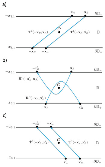
Next, we define the states to which these reciprocity theorems will be applied. For state $A1$ (Figure 4a) we choose a unit source for flux-normalized downgoing waves at ${\mathbf{x}}_A$, just above $\partial {\mathbb{D}}_{-}$. The downgoing field ${\mathbf{p}}_A^{+}$ at $\partial {\mathbb{D}}_{-}$, i.e., just below the source, is $\mathbf{I}\delta ({\mathbf{x}}_{\mathrm{H}}-{\mathbf{x}}_{\mathrm{H},A})$, where ${\mathbf{x}}_{\mathrm{H},A}$ denotes the horizontal coordinates of ${\mathbf{x}}_A$. The upgoing field ${\mathbf{p}}_A^{-}$ at $\partial {\mathbb{D}}_{-}$ is the reflection response ${\mathbf{R}}^{\cup }(\mathbf{x},{\mathbf{x}}_A)$ (the symbol ${\mathbf{R}}^{\cup }$ standing for “reflection from above”) and the downgoing field ${\mathbf{p}}_A^{+}$ at $\partial {\mathbb{D}}_{+}$ is the transmission response ${\mathbf{T}}^{\downarrow }(\mathbf{x},{\mathbf{x}}_A)$. At $\partial {\mathbb{D}}_{+}$ there is no upgoing field. The fields in state $A1$ are summarized in the upper-left part of Table 2. For state $A2$ (Figure 4b) we choose a unit source for flux-normalized upgoing waves at ${\mathbf{x}}_A^{\prime }$, just below $\partial {\mathbb{D}}_{+}$. The upgoing field ${\mathbf{p}}_A^{-}$ at $\partial {\mathbb{D}}_{+}$, i.e., just above the source, is $\mathbf{I}\delta ({\mathbf{x}}_{\mathrm{H}}-{\mathbf{x}}_{\mathrm{H},A}^{\prime })$, where ${\mathbf{x}}_{\mathrm{H},A}^{\prime }$ denotes the horizontal coordinates of ${\mathbf{x}}_A^{\prime }$. The downgoing field ${\mathbf{p}}_A^{+}$ at $\partial {\mathbb{D}}_{+}$ is the reflection response ${\mathbf{R}}^{\cap }(\mathbf{x},{\mathbf{x}}_A^{\prime })$ (the symbol ${\mathbf{R}}^{\cap }$ standing for “reflection from below”) and the upgoing field ${\mathbf{p}}_A^{-}$ at $\partial {\mathbb{D}}_{-}$ is the transmission response ${\mathbf{T}}^{\uparrow }(\mathbf{x},{\mathbf{x}}_A^{\prime })$. At $\partial {\mathbb{D}}_{-}$ there is no downgoing field. The fields in state $A2$ are summarized in the lower-left part of Table 2. States $B1$ and $B2$ are defined in the same way, except that all subscripts A are replaced by subscripts B (see the upper-right and lower-right parts of Table 2).

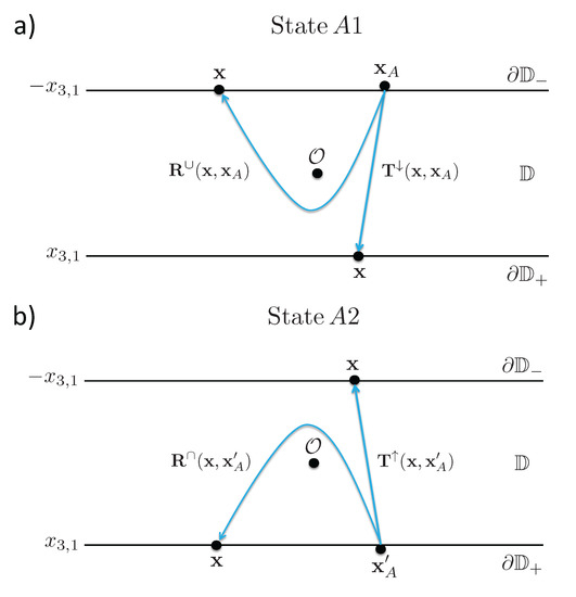
Figure 4. States for the derivation of relations between reflection and transmission responses from reciprocity theorems (56)–(59). (a) State $A1$: the source at ${\mathbf{x}}_A$ is situated just above $\partial {\mathbb{D}}_{-}$. The responses at $\partial {\mathbb{D}}_{-}$ and $\partial {\mathbb{D}}_{+}$ are the reflection response ${\mathbf{R}}^{\cup }(\mathbf{x},{\mathbf{x}}_A)$ and the transmission response ${\mathbf{T}}^{\downarrow }(\mathbf{x},{\mathbf{x}}_A)$. (b) State $A2$: the source at ${\mathbf{x}}_A^{\prime }$ is situated just below $\partial {\mathbb{D}}_{+}$. The responses at $\partial {\mathbb{D}}_{+}$ and $\partial {\mathbb{D}}_{-}$ are the reflection response ${\mathbf{R}}^{\cap }(\mathbf{x},{\mathbf{x}}_A^{\prime })$ and the transmission response ${\mathbf{T}}^{\uparrow }(\mathbf{x},{\mathbf{x}}_A^{\prime })$.

Table 2. States for the derivation of relations between reflection and transmission responses from reciprocity theorems (56)–(59).

State $\mathit{A}1$	${\mathit{p}}_{\mathit{A}}^{+}\left(\mathit{x}\right)$	${\mathit{p}}_{\mathit{A}}^{-}\left(\mathit{x}\right)$	State $\mathit{B}1$	${\mathit{p}}_{\mathit{B}}^{+}\left(\mathit{x}\right)$	${\mathit{p}}_{\mathit{B}}^{-}\left(\mathit{x}\right)$
$\mathbf{x}$ at $\partial {\mathbb{D}}_{-}$	$\mathbf{I}\delta ({\mathbf{x}}_{\mathrm{H}}-{\mathbf{x}}_{\mathrm{H},A})$	${\mathbf{R}}^{\cup }(\mathbf{x},{\mathbf{x}}_A)$	$\mathbf{x}$ at $\partial {\mathbb{D}}_{-}$	$\mathbf{I}\delta ({\mathbf{x}}_{\mathrm{H}}-{\mathbf{x}}_{\mathrm{H},B})$	${\mathbf{R}}^{\cup }(\mathbf{x},{\mathbf{x}}_B)$
$\mathbf{x}$ at $\partial {\mathbb{D}}_{+}$	${\mathbf{T}}^{\downarrow }(\mathbf{x},{\mathbf{x}}_A)$	$\mathbf{O}$	$\mathbf{x}$ at $\partial {\mathbb{D}}_{+}$	${\mathbf{T}}^{\downarrow }(\mathbf{x},{\mathbf{x}}_B)$	$\mathbf{O}$
State $A2$	${\mathbf{p}}_A^{+}\left(\mathbf{x}\right)$	${\mathbf{p}}_A^{-}\left(\mathbf{x}\right)$	State $B2$	${\mathbf{p}}_B^{+}\left(\mathbf{x}\right)$	${\mathbf{p}}_B^{-}\left(\mathbf{x}\right)$
$\mathbf{x}$ at $\partial {\mathbb{D}}_{-}$	$\mathbf{O}$	${\mathbf{T}}^{\uparrow }(\mathbf{x},{\mathbf{x}}_A^{\prime })$	$\mathbf{x}$ at $\partial {\mathbb{D}}_{-}$	$\mathbf{O}$	${\mathbf{T}}^{\uparrow }(\mathbf{x},{\mathbf{x}}_B^{\prime })$
$\mathbf{x}$ at $\partial {\mathbb{D}}_{+}$	${\mathbf{R}}^{\cap }(\mathbf{x},{\mathbf{x}}_A^{\prime })$	$\mathbf{I}\delta ({\mathbf{x}}_{\mathrm{H}}-{\mathbf{x}}_{\mathrm{H},A}^{\prime })$	$\mathbf{x}$ at $\partial {\mathbb{D}}_{+}$	${\mathbf{R}}^{\cap }(\mathbf{x},{\mathbf{x}}_B^{\prime })$	$\mathbf{I}\delta ({\mathbf{x}}_{\mathrm{H}}-{\mathbf{x}}_{\mathrm{H},B}^{\prime })$

In the following derivations, keep in mind that ${\mathbf{x}}_A$ and ${\mathbf{x}}_B$ are both just above $\partial {\mathbb{D}}_{-}$, whereas ${\mathbf{x}}_A^{\prime }$ and ${\mathbf{x}}_B^{\prime }$ are both just below $\partial {\mathbb{D}}_{+}$. Consequently, $-{\mathbf{x}}_A$ and $-{\mathbf{x}}_B$ are both just below $\partial {\mathbb{D}}_{+}$, whereas $-{\mathbf{x}}_A^{\prime }$ and $-{\mathbf{x}}_B^{\prime }$ are both just above $\partial {\mathbb{D}}_{-}$. Finally, when variable $\mathbf{x}$ is at $\partial {\mathbb{D}}_{-}$, then $-\mathbf{x}$ is at $\partial {\mathbb{D}}_{+}$ and vice versa.

We substitute combinations of A and B states into the reciprocity theorems (56)–(59). We start with substitutions in reciprocity theorem (56). Substituting states $A1$ and $B1$ yields

$$\begin{array}{c}\hfill {\mathbf{R}}^{\cup }({\mathbf{x}}_A,{\mathbf{x}}_B)={\left\{{\mathbf{R}}^{\cup }({\mathbf{x}}_B,{\mathbf{x}}_A)\right\}}^t.\end{array}$$

(60)

States $A1$ and $B2$ substituted into Equation (56) yields

$$\begin{array}{c}\hfill {\mathbf{T}}^{\uparrow }({\mathbf{x}}_A,{\mathbf{x}}_B^{\prime })={\left\{{\mathbf{T}}^{\downarrow }({\mathbf{x}}_B^{\prime },{\mathbf{x}}_A)\right\}}^t.\end{array}$$

(61)

Substitution of states $A2$ and $B1$ yields a redundant relation which is not given here. Finally, substitution of states $A2$ and $B2$ into Equation (56) yields

$$\begin{array}{c}\hfill {\mathbf{R}}^{\cap }({\mathbf{x}}_A^{\prime },{\mathbf{x}}_B^{\prime })={\left\{{\mathbf{R}}^{\cap }({\mathbf{x}}_B^{\prime },{\mathbf{x}}_A^{\prime })\right\}}^t.\end{array}$$

(62)

Equations (60)–(62) are the source-receiver reciprocity relations for flux-normalised reflection and transmission responses of an arbitrary inhomogeneous medium [33].

Next, we use reciprocity theorem (59) to derive additional source-receiver reciprocity relations for these responses in a medium with $\mathcal{PT}$-symmetry. Substituting state $A1$ (in the adjoint medium) and state $B1$ (in the original medium) yields

$$\begin{array}{c}\hfill {\mathbf{T}}^{\downarrow }(-{\mathbf{x}}_A,{\mathbf{x}}_B)={\left\{{\overline{\mathbf{T}}}^{\downarrow }(-{\mathbf{x}}_B,{\mathbf{x}}_A)\right\}}^t.\end{array}$$

(63)

State $A1$ (in the adjoint medium) and state $B2$ substituted into Equation (59) yields

$$\begin{array}{c}\hfill {\mathbf{R}}^{\cap }(-{\mathbf{x}}_A,{\mathbf{x}}_B^{\prime })={\left\{{\overline{\mathbf{R}}}^{\cup }(-{\mathbf{x}}_B^{\prime },{\mathbf{x}}_A)\right\}}^t.\end{array}$$

(64)

We skip the redundant relation which is obtained by substituting states $A2$ and state $B1$. Finally, substitution of state $A2$ (in the adjoint medium) and state $B2$ into Equation (59) yields

$$\begin{array}{c}\hfill {\mathbf{T}}^{\uparrow }(-{\mathbf{x}}_A^{\prime },{\mathbf{x}}_B^{\prime })={\left\{{\overline{\mathbf{T}}}^{\uparrow }(-{\mathbf{x}}_B^{\prime },{\mathbf{x}}_A^{\prime })\right\}}^t.\end{array}$$

(65)

Equations (63)–(65) are illustrated in Figure 5.

Figure 5. Additional source-receiver reciprocity of transmission and reflection responses for a medium with $\mathcal{PT}$-symmetry. (a) Equation (63). (b) Equation (64). (c) Equation (65).

Next, we derive two relations using reciprocity theorem (58). Substitution of state $A1$ (in the adjoint medium) and state $B1$ yields

$$\begin{array}{ccc}& & {\int }_{\partial {\mathbb{D}}_{+}}{\left\{{\overline{\mathbf{T}}}^{\downarrow }(\mathbf{x},{\mathbf{x}}_A)\right\}}^{†}{\mathbf{T}}^{\downarrow }(\mathbf{x},{\mathbf{x}}_B){\mathrm{d}}^2{\mathbf{x}}_{\mathrm{H}}=\mathbf{I}\delta ({\mathbf{x}}_{\mathrm{H},A}-{\mathbf{x}}_{\mathrm{H},B})-{\int }_{\partial {\mathbb{D}}_{-}}{\left\{{\overline{\mathbf{R}}}^{\cup }(\mathbf{x},{\mathbf{x}}_A)\right\}}^{†}{\mathbf{R}}^{\cup }(\mathbf{x},{\mathbf{x}}_B){\mathrm{d}}^2{\mathbf{x}}_{\mathrm{H}}.\hfill \end{array}$$

(66)

This relation is a generalisation to an arbitrary inhomogeneous medium of the 1D energy conservation relation $|T^{\downarrow }{|}^2=1-{\left|R^{\cup }\right|}^2$ for a lossless layered medium. In its general form it can be used to derive properties of the transmission response from the reflection response measured at $\partial {\mathbb{D}}_{-}$. Substituting state $A1$ (in the adjoint medium) and state $B2$ into Equation (58) yields

$$\begin{array}{ccc}& & {\int }_{\partial {\mathbb{D}}_{-}}{\left\{{\overline{\mathbf{R}}}^{\cup }(\mathbf{x},{\mathbf{x}}_A)\right\}}^{†}{\mathbf{T}}^{\uparrow }(\mathbf{x},{\mathbf{x}}_B^{\prime }){\mathrm{d}}^2{\mathbf{x}}_{\mathrm{H}}=-{\int }_{\partial {\mathbb{D}}_{+}}{\left\{{\overline{\mathbf{T}}}^{\downarrow }(\mathbf{x},{\mathbf{x}}_A)\right\}}^{†}{\mathbf{R}}^{\cap }(\mathbf{x},{\mathbf{x}}_B^{\prime }){\mathrm{d}}^2{\mathbf{x}}_{\mathrm{H}}.\hfill \end{array}$$

(67)

This expression relates reflection and transmission responses of an arbitrary inhomogeneous medium. Substitution of other combinations of the states in Table 2 into Equation (58) yields relations similar to Equations (66) and (67), which are not explicitly give here.

Finally, we derive two more relations for media with $\mathcal{PT}$-symmetry, using reciprocity theorem (57). Substitution of states $A1$ and $B1$ yields the following relation between reflection and transmission responses

$$\begin{array}{ccc}& & {\int }_{\partial {\mathbb{D}}_{-}}{\left\{{\mathbf{T}}^{\downarrow }(-\mathbf{x},{\mathbf{x}}_A)\right\}}^{†}{\mathbf{R}}^{\cup }(\mathbf{x},{\mathbf{x}}_B){\mathrm{d}}^2{\mathbf{x}}_{\mathrm{H}}=-{\int }_{\partial {\mathbb{D}}_{+}}{\left\{{\mathbf{R}}^{\cup }(-\mathbf{x},{\mathbf{x}}_A)\right\}}^{†}{\mathbf{T}}^{\downarrow }(\mathbf{x},{\mathbf{x}}_B){\mathrm{d}}^2{\mathbf{x}}_{\mathrm{H}},\hfill \end{array}$$

(68)

whereas substitution of states $A1$ and $B2$ gives

$$\begin{array}{ccc}& & {\int }_{\partial {\mathbb{D}}_{-}}{\left\{{\mathbf{T}}^{\downarrow }(-\mathbf{x},{\mathbf{x}}_A)\right\}}^{†}{\mathbf{T}}^{\uparrow }(\mathbf{x},{\mathbf{x}}_B^{\prime }){\mathrm{d}}^2{\mathbf{x}}_{\mathrm{H}}=\mathbf{I}\delta (-{\mathbf{x}}_{\mathrm{H},A}-{\mathbf{x}}_{\mathrm{H},B}^{\prime })-{\int }_{\partial {\mathbb{D}}_{+}}{\left\{{\mathbf{R}}^{\cup }(-\mathbf{x},{\mathbf{x}}_A)\right\}}^{†}{\mathbf{R}}^{\cap }(\mathbf{x},{\mathbf{x}}_B^{\prime }){\mathrm{d}}^2{\mathbf{x}}_{\mathrm{H}}.\hfill \end{array}$$

(69)

The latter expression is a generalisation to an inhomogeneous $\mathcal{PT}$-symmetric medium of the 1D unitarity relation $|T^{\downarrow }{|}^2=1-R^{\cup *}{R}^{\cap }$ for a layered $\mathcal{PT}$-symmetric medium [3,8]. Substitution of other combinations of states into Equation (57) gives similar relations, which will not be discussed.

7. Marchenko Method for $\mathcal{PT}$ Media with Double-Sided Access

Building on work by Marchenko [69], geophysicists recently developed a methodology to retrieve the wave field inside a 3D inhomogeneous medium from reflection measurements at its boundary [34,70,71,72,73,74,75,76]. Underlying this methodology are representations for Green’s functions in terms of the reflection response and focusing functions [35,36]. Here we review these representations, modify them for $\mathcal{PT}$-symmetric media, discuss a modified Marchenko method and illustrate it with a simple numerical example.

We define a focal point ${\mathbf{x}}_F=(x_{1,F},x_{2,F},x_{3,F})$, with $x_{3,F}$ somewhere between $-x_{3,1}$ and $x_{3,1}$. We will apply the reciprocity theorems (56) and (58) to a modified domain, enclosed by $\partial {\mathbb{D}}_{-}$ and $\partial {\mathbb{D}}_F$, with the latter boundary chosen at $x_{3,F}$ (hence, we replace $\partial {\mathbb{D}}_{+}$ by $\partial {\mathbb{D}}_F$ in these reciprocity theorems, see Appendix B for further details). For state A (Figure 6a) we choose again a unit source for flux-normalized downgoing waves at ${\mathbf{x}}_A$, just above $\partial {\mathbb{D}}_{-}$. The downgoing field ${\mathbf{p}}_A^{+}$ at $\partial {\mathbb{D}}_{-}$, i.e., just below the source, is $\mathbf{I}\delta ({\mathbf{x}}_{\mathrm{H}}-{\mathbf{x}}_{\mathrm{H},A})$ and the upgoing field ${\mathbf{p}}_A^{-}$ at $\partial {\mathbb{D}}_{-}$ is the reflection response ${\mathbf{R}}^{\cup }(\mathbf{x},{\mathbf{x}}_A)$. The response at $\partial {\mathbb{D}}_F$ consists of the downgoing and upgoing parts of Green’s matrix, i.e., ${\mathbf{G}}^{+}(\mathbf{x},{\mathbf{x}}_A)$ and ${\mathbf{G}}^{-}(\mathbf{x},{\mathbf{x}}_A)$, respectively. The fields in state A are summarized in the left part of Table 3. For state B (Figure 6b) we choose a flux-normalized focusing matrix ${\mathbf{f}}_1(\mathbf{x},{\mathbf{x}}_F)$ defined in a medium which is reflection-free below the focusing depth level $\partial {\mathbb{D}}_F$. At $\partial {\mathbb{D}}_{-}$ this focusing matrix consists of downgoing and upgoing parts ${\mathbf{f}}_1^{+}(\mathbf{x},{\mathbf{x}}_F)$ and ${\mathbf{f}}_1^{-}(\mathbf{x},{\mathbf{x}}_F)$, respectively. It is defined such that it focuses at $\partial {\mathbb{D}}_F$, hence ${\mathbf{f}}_1^{+}(\mathbf{x},{\mathbf{x}}_F)=\mathbf{I}\delta ({\mathbf{x}}_{\mathrm{H}}-{\mathbf{x}}_{\mathrm{H},F})$ for $\mathbf{x}$ at $\partial {\mathbb{D}}_F$, where ${\mathbf{x}}_{\mathrm{H},F}$ denotes the horizontal coordinates of ${\mathbf{x}}_F$. Since the medium below $\partial {\mathbb{D}}_F$ is reflection-free for the focusing matrix, we have ${\mathbf{f}}_1^{-}(\mathbf{x},{\mathbf{x}}_F)=\mathbf{O}$ for $\mathbf{x}$ at $\partial {\mathbb{D}}_F$. The fields in state B are summarized in the right part of Table 3.

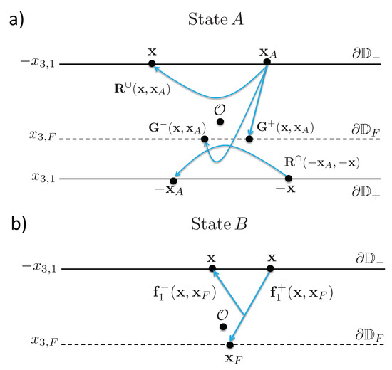
Figure 6. States for the derivation of Marchenko-type representations. (a) State A: the source at ${\mathbf{x}}_A$ is situated just above $\partial {\mathbb{D}}_{-}$. The response at $\partial {\mathbb{D}}_{-}$ is the reflection response ${\mathbf{R}}^{\cup }(\mathbf{x},{\mathbf{x}}_A)$ and the response at the focal depth level $\partial {\mathbb{D}}_F$ consists of the downgoing and upgoing Green’s matrices ${\mathbf{G}}^{+}(\mathbf{x},{\mathbf{x}}_A)$ and ${\mathbf{G}}^{-}(\mathbf{x},{\mathbf{x}}_A)$, respectively. (b) State B: the focal point ${\mathbf{x}}_F$ is situated at $\partial {\mathbb{D}}_F$. At $\partial {\mathbb{D}}_{-}$ the focusing matrix consists of downgoing and upgoing parts ${\mathbf{f}}_1^{+}(\mathbf{x},{\mathbf{x}}_F)$ and ${\mathbf{f}}_1^{-}(\mathbf{x},{\mathbf{x}}_F)$, respectively. The medium below $\partial {\mathbb{D}}_F$ is reflection-free for this state.

Table 3. States for the derivation of Marchenko-type representations.

State A	${\mathit{p}}_{\mathit{A}}^{+}\left(\mathit{x}\right)$	${\mathit{p}}_{\mathit{A}}^{-}\left(\mathit{x}\right)$	State B	${\mathit{p}}_{\mathit{B}}^{+}\left(\mathit{x}\right)$	${\mathit{p}}_{\mathit{B}}^{-}\left(\mathit{x}\right)$
$\mathbf{x}$ at $\partial {\mathbb{D}}_{-}$	$\mathbf{I}\delta ({\mathbf{x}}_{\mathrm{H}}-{\mathbf{x}}_{\mathrm{H},A})$	${\mathbf{R}}^{\cup }(\mathbf{x},{\mathbf{x}}_A)$	$\mathbf{x}$ at $\partial {\mathbb{D}}_{-}$	${\mathbf{f}}_1^{+}(\mathbf{x},{\mathbf{x}}_F)$	${\mathbf{f}}_1^{-}(\mathbf{x},{\mathbf{x}}_F)$
$\mathbf{x}$ at $\partial {\mathbb{D}}_F$	${\mathbf{G}}^{+}(\mathbf{x},{\mathbf{x}}_A)$	${\mathbf{G}}^{-}(\mathbf{x},{\mathbf{x}}_A)$	$\mathbf{x}$ at $\partial {\mathbb{D}}_F$	$\mathbf{I}\delta ({\mathbf{x}}_{\mathrm{H}}-{\mathbf{x}}_{\mathrm{H},F})$	O

Substituting states A and B into Equation (56) (with $\partial {\mathbb{D}}_{+}$ replaced by $\partial {\mathbb{D}}_F$) yields

$$\begin{array}{ccc}& & {\left\{{\mathbf{G}}^{-}({\mathbf{x}}_F,{\mathbf{x}}_A)\right\}}^t+{\mathbf{f}}_1^{-}({\mathbf{x}}_A,{\mathbf{x}}_F)={\int }_{\partial {\mathbb{D}}_{-}}{\left\{{\mathbf{R}}^{\cup }(\mathbf{x},{\mathbf{x}}_A)\right\}}^t{\mathbf{f}}_1^{+}(\mathbf{x},{\mathbf{x}}_F){\mathrm{d}}^2{\mathbf{x}}_{\mathrm{H}}.\hfill \end{array}$$

(70)

Substitution of state A (in the adjoint medium) and state B into Equation (58) yields

$$\begin{array}{ccc}& & -{\left\{{\overline{\mathbf{G}}}^{+}({\mathbf{x}}_F,{\mathbf{x}}_A)\right\}}^{†}+{\mathbf{f}}_1^{+}({\mathbf{x}}_A,{\mathbf{x}}_F)={\int }_{\partial {\mathbb{D}}_{-}}{\left\{{\overline{\mathbf{R}}}^{\cup }(\mathbf{x},{\mathbf{x}}_A)\right\}}^{†}{\mathbf{f}}_1^{-}(\mathbf{x},{\mathbf{x}}_F){\mathrm{d}}^2{\mathbf{x}}_{\mathrm{H}}.\hfill \end{array}$$

(71)

In most papers on the Marchenko method, the medium is assumed lossless. In that case the adjoint medium is the same as the actual medium, meaning that the bars in Equation (71) can be omitted; hence, one-and-the-same reflection response ${\mathbf{R}}^{\cup }(\mathbf{x},{\mathbf{x}}_A)$ appears in Equations (70) and (71). Slob [77] extended the Marchenko method for dissipative media, using (scalar versions of) Equations (70) and (71), including the bars. His method requires the reflection response ${\mathbf{R}}^{\cup }(\mathbf{x},{\mathbf{x}}_A)$ in the actual (dissipative) medium and ${\overline{\mathbf{R}}}^{\cup }(\mathbf{x},{\mathbf{x}}_A)$ in the adjoint (effectual) medium. The former is obtained from measurements, the latter has to be obtained in a different way. Slob [77] proposes to measure the reflection response ${\mathbf{R}}^{\cap }$ from below (next to the reflection response ${\mathbf{R}}^{\cup }$ from above), and the transmission responses ${\mathbf{T}}^{\downarrow }$ and ${\mathbf{T}}^{\uparrow }$. Having these responses, ${\overline{\mathbf{R}}}^{\cup }$ can be obtained by solving Equations (66) and (67). Cui et al. [78] applied this method successfully to acoustic responses of a dissipative medium.

For $\mathcal{PT}$-symmetric media, ${\overline{\mathbf{R}}}^{\cup }$ at $\partial {\mathbb{D}}_{-}$ can be obtained directly from ${\mathbf{R}}^{\cap }$ at $\partial {\mathbb{D}}_{+}$ (Figure 6a), using Equation (64). Substituting this into Equation (71) (and Equation (60) into Equation (70)) yields

$$\begin{array}{ccc}& & {\left\{{\mathbf{G}}^{-}({\mathbf{x}}_F,{\mathbf{x}}_A)\right\}}^t+{\mathbf{f}}_1^{-}({\mathbf{x}}_A,{\mathbf{x}}_F)={\int }_{\partial {\mathbb{D}}_{-}}{\mathbf{R}}^{\cup }({\mathbf{x}}_A,\mathbf{x}){\mathbf{f}}_1^{+}(\mathbf{x},{\mathbf{x}}_F){\mathrm{d}}^2{\mathbf{x}}_{\mathrm{H}}\hfill \end{array}$$

(72)

and

$$\begin{array}{ccc}& & -{\left\{{\overline{\mathbf{G}}}^{+}({\mathbf{x}}_F,{\mathbf{x}}_A)\right\}}^{†}+{\mathbf{f}}_1^{+}({\mathbf{x}}_A,{\mathbf{x}}_F)={\int }_{\partial {\mathbb{D}}_{-}}{\left\{{\mathbf{R}}^{\cap }(-{\mathbf{x}}_A,-\mathbf{x})\right\}}^{*}{\mathbf{f}}_1^{-}(\mathbf{x},{\mathbf{x}}_F){\mathrm{d}}^2{\mathbf{x}}_{\mathrm{H}}.\hfill \end{array}$$

(73)

Equations (72) and (73) form the basis for the Marchenko method in a $\mathcal{PT}$-symmetric medium. The approach is similar to that for lossy media [77], except that here we have replaced ${\overline{\mathbf{R}}}^{\cup }$ by ${\mathbf{R}}^{\cap }$. Starting with an estimate of the direct arrival of the focusing matrix, ${\mathbf{f}}_{1,\mathrm{d}}^{+}$, the Marchenko method leads to the retrieval of ${\mathbf{G}}^{-}$ and ${\overline{\mathbf{G}}}^{+}$, the latter in the adjoint medium. To retrieve ${\mathbf{G}}^{+}$ in the actual medium, we need a second set of equations. To this end, we replace all quantities in Equations (72) and (73) by quantities in the adjoint medium (which implies that ${\overline{\mathbf{G}}}^{+}$ is replaced by ${\mathbf{G}}^{+}$). Using Equations (60) and (64) this yields

$$\begin{array}{ccc}& & {\left\{{\overline{\mathbf{G}}}^{-}({\mathbf{x}}_F,{\mathbf{x}}_A)\right\}}^t+{\overline{\mathbf{f}}}_1^{-}({\mathbf{x}}_A,{\mathbf{x}}_F)={\int }_{\partial {\mathbb{D}}_{-}}{\mathbf{R}}^{\cap }(-{\mathbf{x}}_A,-\mathbf{x}){\overline{\mathbf{f}}}_1^{+}(\mathbf{x},{\mathbf{x}}_F){\mathrm{d}}^2{\mathbf{x}}_{\mathrm{H}}\hfill \end{array}$$

(74)

and

$$\begin{array}{ccc}& & -{\left\{{\mathbf{G}}^{+}({\mathbf{x}}_F,{\mathbf{x}}_A)\right\}}^{†}+{\overline{\mathbf{f}}}_1^{+}({\mathbf{x}}_A,{\mathbf{x}}_F)={\int }_{\partial {\mathbb{D}}_{-}}{\left\{{\mathbf{R}}^{\cup }({\mathbf{x}}_A,\mathbf{x})\right\}}^{*}{\overline{\mathbf{f}}}_1^{-}(\mathbf{x},{\mathbf{x}}_F){\mathrm{d}}^2{\mathbf{x}}_{\mathrm{H}}.\hfill \end{array}$$

(75)

Starting with an estimate of ${\overline{\mathbf{f}}}_{1,\mathrm{d}}^{+}$, the Marchenko method leads to the retrieval of ${\overline{\mathbf{G}}}^{-}$ and ${\mathbf{G}}^{+}$.

We illustrate this with a numerical example for electromagnetic waves in a horizontally layered $\mathcal{PT}$-symmetric medium. Figure 7a shows the relative permittivity ${\epsilon }_{\mathrm{r}}\left(x_3\right)=\epsilon \left(x_3\right)/{\epsilon }_0$ (with ${\epsilon }_0$ the permittivity of vacuum) and Figure 7b the conductivity $\sigma \left(x_3\right)$. Both functions are chosen real-valued and frequency-independent. Note that ${\epsilon }_{\mathrm{r}}\left(x_3\right)$ is symmetric and $\sigma \left(x_3\right)$ is asymmetric. Hence, for $\mathcal{E}$ defined in Equation (6) we have $\mathcal{E}(-x_3,\omega )={\mathcal{E}}^{*}(x_3,\omega )=\overline{\mathcal{E}}(x_3,\omega )$, meaning that Equation (11) is satisfied. The relative permeability ${\mu }_{\mathrm{r}}\left(x_3\right)$ is set to ${\mu }_{\mathrm{r}}=1$.

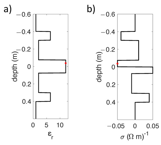
Figure 7. Parameters of a horizontally layered $\mathcal{PT}$-symmetric medium. The red stars indicate the focal depth $x_{3,F}$.

We define the spatial Fourier transform of a space- and frequency-dependent function $u(\mathbf{x},\omega )$ along the horizontal coordinate vector ${\mathbf{x}}_{\mathrm{H}}$ as

$$\begin{array}{ccc}& & \tilde{u}(\mathbf{s},x_3,\omega )={\int }_{{\mathbb{R}}^2}exp\{-i\omega \mathbf{s}·{\mathbf{x}}_{\mathrm{H}}\}u({\mathbf{x}}_{\mathrm{H}},x_3,\omega ){\mathrm{d}}^2{\mathbf{x}}_{\mathrm{H}},\hfill \end{array}$$

(76)

with $\mathbf{s}=(s_1,s_2)$, where $s_1$ and $s_2$ are horizontal slownesses and $\mathbb{R}$ is the set of real numbers. Moreover, we define the inverse Fourier transform from frequency $\omega$ to intercept time $\tau$ as [79]

$$\begin{array}{c}\hfill u(\mathbf{s},x_3,\tau )=\frac{1}{\pi }\Re {\int }_0^{\infty }\tilde{u}(\mathbf{s},x_3,\omega )exp\{-i\omega \tau \}\mathrm{d}\omega .\end{array}$$

(77)

Applying these transforms to Equations (72)–(75) for ${\mathbf{x}}_F=(0,0,x_{3,F})$ and ${\mathbf{x}}_A=({\mathbf{x}}_{\mathrm{H},A},-x_{3,1})$ with variable ${\mathbf{x}}_{\mathrm{H},A}$, yields

$$\begin{array}{ccc}\hfill {\left\{{\mathbf{G}}^{-}(-\mathbf{s},x_{3,F},-x_{3,1},\tau )\right\}}^t+{\mathbf{f}}_1^{-}(\mathbf{s},-x_{3,1},x_{3,F},\tau )& =& {\int }_0^{\infty }{\mathbf{R}}^{\cup }(\mathbf{s},-x_{3,1},{\tau }^{\prime }){\mathbf{f}}_1^{+}(\mathbf{s},-x_{3,1},x_{3,F},\tau -{\tau }^{\prime })\mathrm{d}{\tau }^{\prime },\hfill \end{array}$$

(78)

$$\begin{array}{ccc}\hfill -{\left\{{\overline{\mathbf{G}}}^{+}(\mathbf{s},x_{3,F},-x_{3,1},-\tau )\right\}}^t+{\mathbf{f}}_1^{+}(\mathbf{s},-x_{3,1},x_{3,F},\tau )& =& {\int }_0^{\infty }{\mathbf{R}}^{\cap }(\mathbf{s},x_{3,1},{\tau }^{\prime }){\mathbf{f}}_1^{-}(\mathbf{s},-x_{3,1},x_{3,F},\tau +{\tau }^{\prime })\mathrm{d}{\tau }^{\prime },\hfill \end{array}$$

(79)

$$\begin{array}{ccc}\hfill {\left\{{\overline{\mathbf{G}}}^{-}(-\mathbf{s},x_{3,F},-x_{3,1},\tau )\right\}}^t+{\overline{\mathbf{f}}}_1^{-}(\mathbf{s},-x_{3,1},x_{3,F},\tau )& =& {\int }_0^{\infty }{\mathbf{R}}^{\cap }(-\mathbf{s},x_{3,1},{\tau }^{\prime }){\overline{\mathbf{f}}}_1^{+}(\mathbf{s},-x_{3,1},x_{3,F},\tau -{\tau }^{\prime })\mathrm{d}{\tau }^{\prime },\hfill \end{array}$$

(80)

$$\begin{array}{ccc}\hfill -{\left\{{\mathbf{G}}^{+}(\mathbf{s},x_{3,F},-x_{3,1},-\tau )\right\}}^t+{\overline{\mathbf{f}}}_1^{+}(\mathbf{s},-x_{3,1},x_{3,F},\tau )& =& {\int }_0^{\infty }{\mathbf{R}}^{\cup }(-\mathbf{s},-x_{3,1},{\tau }^{\prime }){\overline{\mathbf{f}}}_1^{-}(\mathbf{s},-x_{3,1},x_{3,F},\tau +{\tau }^{\prime })\mathrm{d}{\tau }^{\prime }.\hfill \end{array}$$

(81)

Taking the horizontal slowness $s_2$ equal to 0, the transverse-electric (TE) mode decouples from the transverse-magnetic (TM) mode. Consequently, the matrices in Equations (78)–(81) diagonalize. We continue with the upper-left elements of these matrices, which correspond to the up/down decomposed TE-mode. We use the reflectivity method [80] to model the response of the medium. Figure 8a shows the scalar reflection response from above, $R^{\cup }(s_1,-x_{3,1},\tau )$, for $-x_{3,1}=-0.6$ m, as a function of intercept time $\tau$ and incidence angle $\theta$. The latter is related to the horizontal slowness $s_1$ via $\frac{sin\theta }{c}=s_1$, with c the propagation velocity at $-x_{3,1}=-0.6$ m (which is equal to the velocity of light in vacuum, since ${\epsilon }_{\mathrm{r}}={\mu }_{\mathrm{r}}=1$ at $-x_{3,1}=-0.6$ m). Similarly, Figure 8b shows the scalar reflection response from below, $R^{\cap }(s_1,x_{3,1},\tau )$, for $x_{3,1}=0.6$ m. Both responses have been convolved with a symmetric source function with a central frequency of 2 GHz. Our aim is to use the Marchenko method to find the downgoing and upgoing parts of Green’s function, $G^{+}(s_1,x_{3,F},-x_{3,1},\tau )$ and $G^{-}(s_1,x_{3,F},-x_{3,1},\tau )$, between $-x_{3,1}=-0.6$ m and an arbitrary focal depth $x_{3,F}$ inside the medium, from the reflection responses $R^{\cup }$ and $R^{\cap }$. We discuss the main steps; for details on the Marchenko method, see the references at the beginning of this section. For this example we choose the focal depth as $x_{3,F}=-3.75$ cm (indicated by the red stars in Figure 7). We apply a time window to suppress Green’s functions from Equations (78)–(), which leaves equations for the focusing functions $f_1^{+}$, $f_1^{-}$, ${\overline{f}}_1^{+}$ and ${\overline{f}}_1^{-}$. We model the direct arrival $f_{1,\mathrm{d}}^{+}$ in the medium of Figure 7. Using this direct arrival as an initial estimate of $f_1^{+}$, the windowed versions of Equations (78) and (79) are iteratively solved for $f_1^{+}$ and $f_1^{-}$. Once these are found, the original versions of Equations (78) and (79) (i.e., without the time window) yield estimates of $G^{-}$ and ${\overline{G}}^{+}$. Next, we model the direct arrival ${\overline{f}}_{1,\mathrm{d}}^{+}$ in the adjoint of the medium of Figure 7 and use windowed versions of Equations (80) and (81) to solve for ${\overline{f}}_1^{+}$ and ${\overline{f}}_1^{-}$ and, subsequently, retrieve estimates of ${\overline{G}}^{-}$ and $G^{+}$. The results $G^{+}$ and $G^{-}$ are shown by the red-dashed lines in Figure 9a,b, respectively. The first arrival in $G^{+}$ comes from ${\overline{f}}_{1,\mathrm{d}}^{+}$; all other (multiply reflected) arrivals in $G^{+}$ and $G^{-}$ have been retrieved from $R^{\cup }$ and $R^{\cap }$. The results are overlain on the directly modelled versions of $G^{+}$ and $G^{-}$, obtained with the reflectivity method (black solid lines). Note that the match is excellent.

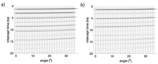
Figure 8. (a) Reflection response from above, $R^{\cup }(s_1,-x_{3,1},\tau )$, for $-x_{3,1}=-0.6$ m. (b) Reflection response from below, $R^{\cap }(s_1,x_{3,1},\tau )$, for $x_{3,1}=0.6$ m.

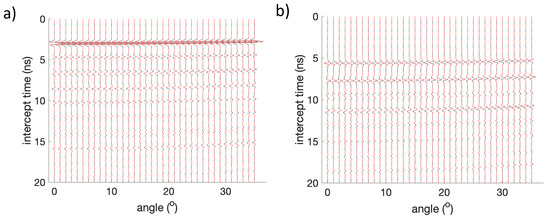
Figure 9. (a) Green’s function $G^{+}(s_1,x_{3,F},-x_{3,1},\tau )$. (b) Green’s function $G^{-}(s_1,x_{3,F},-x_{3,1},\tau )$. The red dashed lines are Green’s functions retrieved with the Marchenko method from $R^{\cup }$ and $R^{\cap }$; the black solid lines are the directly modelled Green’s functions.

8. Discussion and Conclusions

Starting with a unified matrix-vector wave equation for acoustic, quantum-mechanical, electromagnetic, elastodynamic, poroelastodynamic, piezoelectric and seismoelectric waves, we established symmetry properties of the operator matrix appearing in this equation for the situation of 3D arbitrary inhomogeneous media and for 3D inhomogeneous media with $\mathcal{PT}$-symmetry. For the latter situation we obtained an auxiliary matrix-vector wave equation. Exploiting the symmetry properties, we derived four unified reciprocity theorems, two for arbitrary inhomogeneous media and two for inhomogeneous media with $\mathcal{PT}$-symmetry. We used these reciprocity theorems to derive general wave field representations and relations between reflection and transmission responses, for 3D arbitrary inhomogeneous media and for 3D inhomogeneous media with $\mathcal{PT}$-symmetry, embedded between two homogeneous lossless half-spaces. These relations have potential applications in forward and inverse problems in such media, including interferometric Green’s matrix retrieval from passive or active measurements. Finally, we modified the Marchenko method for retrieving Green’s matrices from reflection measurements for 3D inhomogeneous media with $\mathcal{PT}$-symmetry.

Given the current broad interest in applications of wave propagation and scattering in photonic structures, phononic crystals and acoustic metamaterials with $\mathcal{PT}$-symmetry, we hope that our unified formulation for different wave types and our generalisation for 3D inhomogeneous media with $\mathcal{PT}$-symmetry, will contribute to further developments in this interesting field of research.

Appendix A.1. The Wave Vector and Operator Matrix for Different Wave Phenomena

For acoustic waves in an inhomogeneous fluid, p and $v_3$ in Table 1 are the acoustic pressure and the vertical component of the particle velocity, respectively. The $2\times 2$ operator matrix $\mathcal{A}\left(\mathbf{x}\right)$ is defined as [42,81,82,83,84]

$$\begin{array}{ccc}\hfill \mathcal{A}\left(\mathbf{x}\right)& =& \left(\begin{array}{cc}0& i\omega \rho \\ i\omega \kappa -\frac{1}{i\omega }{\partial }_{\alpha }\frac{1}{\rho }{\partial }_{\alpha }& 0\end{array}\right),\hfill \end{array}$$

(A1)

where $\kappa \left(\mathbf{x}\right)$ is the compressibility and $\rho \left(\mathbf{x}\right)$ the mass density. Einstein’s summation convention applies to repeated subscripts.

For quantum-mechanical waves in an inhomogeneous potential, $\psi$ and m in Table 1 are the wave function and the mass of a particle, respectively, and $\hslash =h/2\pi$, with h Planck’s constant. The $2\times 2$ matrix is [28,85,86]

$$\begin{array}{ccc}\hfill \mathcal{A}\left(\mathbf{x}\right)& =& \left(\begin{array}{cc}0& \frac{mi}{2\hslash }\\ 4i\left(\omega -\frac{V}{\hslash }\right)-\frac{2\hslash }{mi}{\partial }_{\alpha }{\partial }_{\alpha }& 0\end{array}\right),\hfill \end{array}$$

(A2)

where $V\left(\mathbf{x}\right)$ is the potential.

For electromagnetic waves in an inhomogeneous, isotropic medium, $E_{\alpha }$ and $H_{\alpha }$ ($\alpha =1,2$) in Table 1 are the horizontal components of the electric and magnetic field strength, respectively. The $2\times 2$ sub-matrices of operator matrix $\mathcal{A}\left(\mathbf{x}\right)$ are given by Equations (4) and (5).

For elastodynamic waves in an inhomogeneous, isotropic solid, $v_k$ and ${\tau }_{k3}$ ($k=1,2,3$) in Table 1 are the particle velocity and traction components, respectively. The $3\times 3$ sub-matrices are [40,42,52]

$$\begin{array}{ccc}\hfill {\mathcal{A}}_{11}\left(\mathbf{x}\right)& =& \left(\begin{array}{ccc}0& 0& -{\partial }_1\\ 0& 0& -{\partial }_2\\ -\frac{\lambda }{\lambda +2\mu }{\partial }_1& -\frac{\lambda }{\lambda +2\mu }{\partial }_2& 0\end{array}\right),\hfill \end{array}$$

(A3)

$$\begin{array}{ccc}\hfill {\mathcal{A}}_{12}\left(\mathbf{x}\right)& =& \left(\begin{array}{ccc}\frac{i\omega }{\mu }& 0& 0\\ 0& \frac{i\omega }{\mu }& 0\\ 0& 0& \frac{i\omega }{\lambda +2\mu }\end{array}\right),\hfill \end{array}$$

(A4)

$$\begin{array}{ccc}\hfill {\mathcal{A}}_{21}\left(\mathbf{x}\right)& =& \left(\begin{array}{ccc}i\omega \rho -\frac{1}{i\omega }\left({\partial }_1{\nu }_1{\partial }_1+{\partial }_2\mu {\partial }_2\right)& -\frac{1}{i\omega }\left({\partial }_2\mu {\partial }_1+{\partial }_1{\nu }_2{\partial }_2\right)& 0\\ -\frac{1}{i\omega }\left({\partial }_2{\nu }_2{\partial }_1+{\partial }_1\mu {\partial }_2\right)& i\omega \rho -\frac{1}{i\omega }\left({\partial }_1\mu {\partial }_1+{\partial }_2{\nu }_1{\partial }_2\right)& 0\\ 0& 0& i\omega \rho \end{array}\right),\hfill \end{array}$$

(A5)

$$\begin{array}{ccc}\hfill {\mathcal{A}}_{22}\left(\mathbf{x}\right)& =& -{\mathcal{A}}_{11}^t\left(\mathbf{x}\right),\hfill \end{array}$$

(A6)

with

$$\begin{array}{c}\hfill {\nu }_1=4\mu \left(\frac{\lambda +\mu }{\lambda +2\mu }\right),{\nu }_2=2\mu \left(\frac{\lambda }{\lambda +2\mu }\right),\end{array}$$

(A7)

where $\lambda \left(\mathbf{x}\right)$ and $\mu \left(\mathbf{x}\right)$ are the Lamé parameters and $\rho \left(\mathbf{x}\right)$ the mass density.

The wave field quantities for the other wave phenomena in Table 1 are the same quantities as above, with superscripts b, f and s denoting that they are averaged in the bulk, fluid or solid, respectively; $\varphi$ denotes porosity. For the sub-matrices for these phenomena we refer to the Appendices in reference [28].

Appendix A.2. Fourier Transform of the Operator Matrix

Consider any depth $x_3$ where the medium is laterally invariant. Applying the spatial Fourier transform of Equation (76) to the operator matrix of Equation (A1) yields

$$\begin{array}{c}\hfill \tilde{\mathbf{A}}(\mathbf{s},x_3)=\left(\begin{array}{cc}0& i\omega \rho \\ i\omega \left(\kappa -\frac{1}{\rho }{s}_{\alpha }{s}_{\alpha }\right)& 0\end{array}\right),\end{array}$$

(A8)

with $\kappa \left(x_3\right)$ and $\rho \left(x_3\right)$ being the laterally invariant compressibility and mass density at $x_3$. Note that ${\partial }_{\alpha }$ has been replaced by $i\omega s_{\alpha }$. The operators for other wave phenomena are transformed in a similar way. The symmetry properties of Equations (7)–(9) transform to

$$\begin{array}{ccc}\hfill {\tilde{\mathbf{A}}}^t(-\mathbf{s},x_3)\mathbf{N}& =& -\mathbf{N}\tilde{\mathbf{A}}(\mathbf{s},x_3),\hfill \end{array}$$

(A9)

$$\begin{array}{ccc}\hfill {\tilde{\mathbf{A}}}^{†}(\mathbf{s},x_3)\mathbf{K}& =& -\mathbf{K}\widetilde{\overline{\mathbf{A}}}(\mathbf{s},x_3),\hfill \end{array}$$

(A10)

$$\begin{array}{ccc}\hfill {\tilde{\mathbf{A}}}^{*}(-\mathbf{s},x_3)\mathbf{J}& =& \mathbf{J}\widetilde{\overline{\mathbf{A}}}(\mathbf{s},x_3).\hfill \end{array}$$

(A11)

In Equations (A1) and (A1), $\widetilde{\overline{\mathbf{A}}}(\mathbf{s},x_3)$ is defined in the adjoint medium.

Appendix A.3. Decomposition of the Transformed Operator Matrix

We define the eigenvalue decomposition of the transformed operator matrix at $x_3$ as

$$\begin{array}{ccc}\hfill \tilde{\mathbf{A}}(\mathbf{s},x_3)& =& \tilde{\mathbf{L}}(\mathbf{s},x_3)\tilde{\Lambda }(\mathbf{s},x_3){\tilde{\mathbf{L}}}^{-1}(\mathbf{s},x_3),\hfill \end{array}$$

(A12)

in which the matrices $\tilde{\mathbf{L}}(\mathbf{s},x_3)$ and $\tilde{\Lambda }(\mathbf{s},x_3)$ are partitioned as follows

$$\begin{array}{c}\hfill \tilde{\mathbf{L}}(\mathbf{s},x_3)=\left(\begin{array}{cc}{\tilde{\mathbf{L}}}_1^{+}& {\tilde{\mathbf{L}}}_1^{-}\\ {\tilde{\mathbf{L}}}_2^{+}& {\tilde{\mathbf{L}}}_2^{-}\end{array}\right),\tilde{\Lambda }(\mathbf{s},x_3)=\left(\begin{array}{cc}{\tilde{\Lambda }}^{+}& \mathbf{O}\\ \mathbf{O}& {\tilde{\Lambda }}^{-}\end{array}\right).\end{array}$$

(A13)

For acoustic waves we have

$$\begin{array}{c}\hfill \tilde{\mathbf{L}}(\mathbf{s},x_3)=\frac{1}{\sqrt{2}}\left(\begin{array}{cc}\sqrt{\rho /s_3}& \sqrt{\rho /s_3}\\ \sqrt{s_3/\rho }& -\sqrt{s_3/\rho }\end{array}\right),\tilde{\Lambda }(\mathbf{s},x_3)=\left(\begin{array}{cc}i\omega s_3& 0\\ 0& -i\omega s_3\end{array}\right),\end{array}$$

(A14)

where $s_3(\mathbf{s},x_3)$ is the vertical slowness at $x_3$, defined as

$$\begin{array}{c}\hfill s_3(\mathbf{s},x_3)=\sqrt{\frac{1}{c^2\left(x_3\right)}-s_{\alpha }{s}_{\alpha }},c\left(x_3\right)=1/\sqrt{\rho \left(x_3\right)\kappa \left(x_3\right)}.\end{array}$$

(A15)

When the medium is dissipative (with, for positive $\omega$, $\Im \left(\kappa \right)>0$ and $\Im \left(\rho \right)>0$), we have $\Im \left(s_3\right)>0$, see Figure A1a. On the other hand, when the medium is effectual (with, for positive $\omega$, $\Im \left(\kappa \right)<0$ and $\Im \left(\rho \right)<0$), we have $\Im \left(s_3\right)<0$, see Figure A1b. Since the parameters of the adjoint medium are defined as $\overline{\kappa }={\kappa }^{*}$ and $\overline{\rho }={\rho }^{*}$, the vertical slowness ${\overline{s}}_3$ of the adjoint medium is given by ${\overline{s}}_3(\mathbf{s},x_3)=s_3^{*}(\mathbf{s},x_3)$.

Figure A1. Slowness $s_3(\mathbf{s},x_3)$ (for any depth $x_3$ where the medium is laterally invariant) in the complex plane for a dissipative (a) and an effectual (b) medium at $x_3$.

Figure A1. Slowness $s_3(\mathbf{s},x_3)$ (for any depth $x_3$ where the medium is laterally invariant) in the complex plane for a dissipative (a) and an effectual (b) medium at $x_3$.

For quantum mechanical waves we have

$$\begin{array}{c}\hfill \tilde{\mathbf{L}}(\mathbf{s},x_3)=\frac{1}{\sqrt{2}}\left(\begin{array}{cc}\sqrt{\frac{m}{2\hslash \omega s_3}}& \sqrt{\frac{m}{2\hslash \omega s_3}}\\ \sqrt{\frac{2\hslash \omega s_3}{m}}& -\sqrt{\frac{2\hslash \omega s_3}{m}}\end{array}\right),\end{array}$$

(A16)

and $\tilde{\Lambda }(\mathbf{s},x_3)$ and $s_3(\mathbf{s},x_3)$ defined as in Equations (A14) and (A15), but with $c\left(x_3\right)$ defined as

$$\begin{array}{c}\hfill c\left(x_3\right)=\sqrt{\frac{\hslash \omega }{2m\left(1-\frac{V\left(x_3\right)}{\hslash \omega }\right)}}.\end{array}$$

(A17)

For electromagnetic waves, the sub-matrices are given by [42]

$$\begin{array}{ccc}\hfill {\tilde{\mathbf{L}}}_1^{\pm }(\mathbf{s},x_3)& =& \frac{1}{\sqrt{2}}\left(\begin{array}{cc}\frac{\sqrt{\mu s_3}}{s_0}& -\frac{s_1{s}_2}{s_0\sqrt{\mathcal{E}{s}_3}}\\ 0& \frac{s_0}{\sqrt{\mathcal{E}{s}_3}}\end{array}\right),{\tilde{\mathbf{L}}}_2^{\pm }(\mathbf{s},x_3)=\pm \frac{1}{\sqrt{2}}\left(\begin{array}{cc}\frac{s_0}{\sqrt{\mu s_3}}& 0\\ \frac{s_1{s}_2}{s_0\sqrt{\mu s_3}}& \frac{\sqrt{\mathcal{E}{s}_3}}{s_0}\end{array}\right),\hfill \end{array}$$

(A18)

$$\begin{array}{ccc}\hfill {\tilde{\Lambda }}^{\pm }(\mathbf{s},x_3)& =& \pm i\omega \left(\begin{array}{cc}{s}_3& 0\\ 0& s_3\end{array}\right),s_0(\mathbf{s},x_3)=\sqrt{\frac{1}{c^2\left(x_3\right)}-s_2^2},\hfill \end{array}$$

(A19)

and $s_3(\mathbf{s},x_3)$ defined as in Equation (A15), but with $c\left(x_3\right)$ defined as $c\left(x_3\right)=1/\sqrt{\mathcal{E}\left(x_3\right)\mu \left(x_3\right)}$.

For elastodynamic waves the sub-matrices of $\tilde{\mathbf{L}}$ and $\tilde{\Lambda }$ are

$$\begin{array}{ccc}& & {\tilde{\mathbf{L}}}_1^{\pm }(\mathbf{s},x_3)=\frac{1}{{\left(2\rho \right)}^{1/2}}\left(\begin{array}{ccc}\frac{s_1}{{\left(s_3^P\right)}^{1/2}}& -\frac{s_1{\left(s_3^S\right)}^{1/2}}{s_r}& -\frac{s_2}{c_S{s}_r{\left(s_3^S\right)}^{1/2}}\\ \frac{s_2}{{\left(s_3^P\right)}^{1/2}}& -\frac{s_2{\left(s_3^S\right)}^{1/2}}{s_r}& \frac{s_1}{c_S{s}_r{\left(s_3^S\right)}^{1/2}}\\ \pm {\left(s_3^P\right)}^{1/2}& \pm \frac{s_r}{{\left(s_3^S\right)}^{1/2}}& 0\end{array}\right),\hfill \end{array}$$

(A20)

$$\begin{array}{ccc}& & {\tilde{\mathbf{L}}}_2^{\pm }(\mathbf{s},x_3)={\left(\frac{\rho }{2}\right)}^{1/2}{c}_S^2\left(\begin{array}{ccc}\pm 2s_1{\left(s_3^P\right)}^{1/2}& \mp \frac{s_1(c_S^{-2}-2s_r^2)}{s_r{\left(s_3^S\right)}^{1/2}}& \mp \frac{s_2{\left(s_3^S\right)}^{1/2}}{c_S{s}_r}\\ \pm 2s_2{\left(s_3^P\right)}^{1/2}& \mp \frac{s_2(c_S^{-2}-2s_r^2)}{s_r{\left(s_3^S\right)}^{1/2}}& \pm \frac{s_1{\left(s_3^S\right)}^{1/2}}{c_S{s}_r}\\ \frac{(c_S^{-2}-2s_r^2)}{{\left(s_3^P\right)}^{1/2}}& 2s_r{\left(s_3^S\right)}^{1/2}& 0\end{array}\right),\hfill \end{array}$$

(A21)

$$\begin{array}{ccc}& & {\tilde{\Lambda }}^{\pm }(\mathbf{s},x_3)=\pm i\omega \left(\begin{array}{ccc}{s}_3^P& 0& 0\\ 0& s_3^S& 0\\ 0& 0& s_3^S\end{array}\right),\hfill \end{array}$$

(A22)

with $s_r=\sqrt{s_1^2+s_2^2}$ and the vertical slownesses $s_3^P$ and $s_3^S$ defined as

$$\begin{array}{c}\hfill s_3^{P,S}(\mathbf{s},x_3)=\sqrt{\frac{1}{c_{P,S}^2\left(x_3\right)}-s_{\alpha }{s}_{\alpha }},\end{array}$$

(A23)

where $c_P\left(x_3\right)$ and $c_S\left(x_3\right)$ are the P- and S-wave velocities, defined as

$c_P\left(x_3\right)=\sqrt{(\lambda \left(x_3\right)+2\mu \left(x_3\right))/\rho \left(x_3\right)}$ and $c_S\left(x_3\right)=\sqrt{\mu \left(x_3\right)/\rho \left(x_3\right)}$, respectively.

For all cases, matrix $\tilde{\mathbf{L}}(\mathbf{s},x_3)$ obeys the following symmetry relations

$$\begin{array}{ccc}\hfill {\tilde{\mathbf{L}}}^t(-\mathbf{s},x_3)\mathbf{N}\tilde{\mathbf{L}}(\mathbf{s},x_3)& =& -\mathbf{N},\hfill \end{array}$$

(A24)

$$\begin{array}{ccc}\hfill {\tilde{\mathbf{L}}}^t(\mathbf{s},x_3)\mathbf{K}\tilde{\mathbf{L}}(\mathbf{s},x_3)& =& \mathbf{J}.\hfill \end{array}$$

(A25)

Using ${\overline{s}}_3(\mathbf{s},x_3)=s_3^{*}(\mathbf{s},x_3)$ etc., we have in addition

$$\begin{array}{ccc}\hfill {\widetilde{\overline{\mathbf{L}}}}^{†}(-\mathbf{s},x_3)\mathbf{N}\tilde{\mathbf{L}}(\mathbf{s},x_3)& =& -\mathbf{N},\hfill \end{array}$$

(A26)

$$\begin{array}{ccc}\hfill {\widetilde{\overline{\mathbf{L}}}}^{†}(\mathbf{s},x_3)\mathbf{K}\tilde{\mathbf{L}}(\mathbf{s},x_3)& =& \mathbf{J}.\hfill \end{array}$$

(A27)

Here $\widetilde{\overline{\mathbf{L}}}(\mathbf{s},x_3)$ is defined in the adjoint medium. Finally, when the medium is lossless at $x_3$, we have $s_3(\mathbf{s},x_3)=s_3^{*}(\mathbf{s},x_3)$ for propagating (i.e., non-evanescent) waves, hence

$$\begin{array}{ccc}\hfill {\tilde{\mathbf{L}}}^{†}(-\mathbf{s},x_3)\mathbf{N}\tilde{\mathbf{L}}(\mathbf{s},x_3)& =& -\mathbf{N},(\mathrm{for} \mathrm{propagating} \mathrm{waves}),\hfill \end{array}$$

(A28)

$$\begin{array}{ccc}\hfill {\tilde{\mathbf{L}}}^{†}(\mathbf{s},x_3)\mathbf{K}\tilde{\mathbf{L}}(\mathbf{s},x_3)& =& \mathbf{J},(\mathrm{for} \mathrm{propagating} \mathrm{waves}).\hfill \end{array}$$

(A29)

Appendix B.4. Boundaries without Losses

Here we present the details behind the analysis of the boundary integrals in Section 4. At and outside the boundary $\partial \mathbb{D}$ the medium is homogeneous, lossless, and identical in both half-spaces and in both states. The boundary integral in Equation (16) consists of two integrals ${\int }_{{\mathbb{R}}^2}{\mathbf{q}}_A^t({\mathbf{x}}_{\mathrm{H}},x_3)\mathbf{N}{\mathbf{q}}_B({\mathbf{x}}_{\mathrm{H}},x_3){\mathrm{d}}^2{\mathbf{x}}_{\mathrm{H}}$, one for $x_3=-x_{3,1}$ and one for $x_3=x_{3,1}$. Using the spatial Fourier transform of Equation (76) and Parseval’s theorem, we obtain for these integrals

$$\begin{array}{c}\hfill {\int }_{{\mathbb{R}}^2}{\mathbf{q}}_A^t({\mathbf{x}}_{\mathrm{H}},x_3)\mathbf{N}{\mathbf{q}}_B({\mathbf{x}}_{\mathrm{H}},x_3){\mathrm{d}}^2{\mathbf{x}}_{\mathrm{H}}=\frac{{\omega }^2}{4{\pi }^2}{\int }_{{\mathbb{R}}^2}{\tilde{\mathbf{q}}}_A^t(-\mathbf{s},x_3)\mathbf{N}{\tilde{\mathbf{q}}}_B(\mathbf{s},x_3){\mathrm{d}}^2\mathbf{s},\end{array}$$

(A30)

for $x_3=-x_{3,1}$ and $x_3=x_{3,1}$. Applying the spatial Fourier transform to Equations (21) and (22), we obtain

$$\begin{array}{ccc}\hfill {\tilde{\mathbf{q}}}_A(\mathbf{s},x_3)& =& \tilde{\mathbf{L}}(\mathbf{s},x_3){\tilde{\mathbf{p}}}_A(\mathbf{s},x_3),\hfill \end{array}$$

(A31)

$$\begin{array}{ccc}\hfill {\tilde{\mathbf{q}}}_B(\mathbf{s},x_3)& =& \tilde{\mathbf{L}}(\mathbf{s},x_3){\tilde{\mathbf{p}}}_B(\mathbf{s},x_3),\hfill \end{array}$$

(A32)

with

$$\begin{array}{c}\hfill {\tilde{\mathbf{p}}}_{A,B}(\mathbf{s},x_3)=\left(\begin{array}{c}{\tilde{\mathbf{p}}}_{A,B}^{+}(\mathbf{s},x_3)\\ {\tilde{\mathbf{p}}}_{A,B}^{-}(\mathbf{s},x_3)\end{array}\right),\end{array}$$

(A33)

where ${\tilde{\mathbf{p}}}_{A,B}^{+}(\mathbf{s},x_3)$ and ${\tilde{\mathbf{p}}}_{A,B}^{-}(\mathbf{s},x_3)$ are downgoing and upgoing plane-wave fields in states A and B at $x_3=-x_{3,1}$ and $x_3=x_{3,1}$. Note that $\tilde{\mathbf{L}}(\mathbf{s},x_3)$ in Equations (A31) and () is without subscript A or B, since the medium at and outside $\partial \mathbb{D}$ is the same in both states. Matrix $\tilde{\mathbf{L}}(\mathbf{s},x_3)$ is given for a number of situations in Appendix A. Substitution of Equations (A31) and (A32) into the right-hand side of Equation (A30) gives

$$\begin{array}{c}\hfill {\int }_{{\mathbb{R}}^2}{\mathbf{q}}_A^t({\mathbf{x}}_{\mathrm{H}},x_3)\mathbf{N}{\mathbf{q}}_B({\mathbf{x}}_{\mathrm{H}},x_3){\mathrm{d}}^2{\mathbf{x}}_{\mathrm{H}}=\frac{{\omega }^2}{4{\pi }^2}{\int }_{{\mathbb{R}}^2}{\tilde{\mathbf{p}}}_A^t(-\mathbf{s},x_3){\tilde{\mathbf{L}}}^t(-\mathbf{s},x_3)\mathbf{N}\tilde{\mathbf{L}}(\mathbf{s},x_3){\tilde{\mathbf{p}}}_B(\mathbf{s},x_3){\mathrm{d}}^2\mathbf{s},\end{array}$$

(A34)

for $x_3=\pm x_{3,1}$. Using symmetry relation (A24) this yields

$$\begin{array}{c}\hfill {\int }_{{\mathbb{R}}^2}{\mathbf{q}}_A^t({\mathbf{x}}_{\mathrm{H}},x_3)\mathbf{N}{\mathbf{q}}_B({\mathbf{x}}_{\mathrm{H}},x_3){\mathrm{d}}^2{\mathbf{x}}_{\mathrm{H}}=-\frac{{\omega }^2}{4{\pi }^2}{\int }_{{\mathbb{R}}^2}{\tilde{\mathbf{p}}}_A^t(-\mathbf{s},x_3)\mathbf{N}{\tilde{\mathbf{p}}}_B(\mathbf{s},x_3){\mathrm{d}}^2\mathbf{s},\end{array}$$

(A35)

for $x_3=\pm x_{3,1}$. Applying Parseval’s theorem to the right-hand side and combining the integrals for $x_3=\pm x_{3,1}$, finally yields

$$\begin{array}{ccc}\hfill {\int }_{\partial \mathbb{D}}{\mathbf{q}}_A^t\left(\mathbf{x}\right)\mathbf{N}{\mathbf{q}}_B\left(\mathbf{x}\right)n_3{\mathrm{d}}^2{\mathbf{x}}_{\mathrm{H}}& =& -{\int }_{\partial \mathbb{D}}{\mathbf{p}}_A^t\left(\mathbf{x}\right)\mathbf{N}{\mathbf{p}}_B\left(\mathbf{x}\right)n_3{\mathrm{d}}^2{\mathbf{x}}_{\mathrm{H}}.\hfill \end{array}$$

(A36)

This is Equation (23) in the main text. Next, for the two integrals in the boundary integral in Equation (17) we obtain, analogous to Equation (A30),

$$\begin{array}{c}\hfill {\int }_{{\mathbb{R}}^2}{\mathbf{q}}_A^{†}(-{\mathbf{x}}_{\mathrm{H}},-x_3)\mathbf{N}{\mathbf{q}}_B({\mathbf{x}}_{\mathrm{H}},x_3){\mathrm{d}}^2{\mathbf{x}}_{\mathrm{H}}=\frac{{\omega }^2}{4{\pi }^2}{\int }_{{\mathbb{R}}^2}{\tilde{\mathbf{q}}}_A^{†}(-\mathbf{s},-x_3)\mathbf{N}{\tilde{\mathbf{q}}}_B(\mathbf{s},x_3){\mathrm{d}}^2\mathbf{s},\end{array}$$

(A37)

for $x_3=-x_{3,1}$ and $x_3=x_{3,1}$. Substitution of Equations (A31) and (A32) into the right-hand side of Equation (A37), using $\tilde{\mathbf{L}}(\mathbf{s},-x_{3,1})=\tilde{\mathbf{L}}(\mathbf{s},x_{3,1})$ (since the medium at and outside $\partial \mathbb{D}$ is the same in both half-spaces) and symmetry relation (A28), applying Parseval’s theorem to the right-hand side and combining the integrals for $x_3=\pm x_{3,1}$, yields

$$\begin{array}{ccc}\hfill {\int }_{\partial \mathbb{D}}{\mathbf{q}}_A^{†}(-\mathbf{x})\mathbf{N}{\mathbf{q}}_B\left(\mathbf{x}\right)n_3{\mathrm{d}}^2{\mathbf{x}}_{\mathrm{H}}& \approx & -{\int }_{\partial \mathbb{D}}{\mathbf{p}}_A^{†}(-\mathbf{x})\mathbf{N}{\mathbf{p}}_B\left(\mathbf{x}\right)n_3{\mathrm{d}}^2{\mathbf{x}}_{\mathrm{H}}.\hfill \end{array}$$

(A38)

This is Equation (24) in the main text. The approximation sign denotes that evanescent waves are ignored at $\partial \mathbb{D}$, see equation Equation (A28).

Next, for the two integrals in the boundary integral in Equation (18) we obtain

$$\begin{array}{c}\hfill {\int }_{{\mathbb{R}}^2}{\mathbf{q}}_A^{†}({\mathbf{x}}_{\mathrm{H}},x_3)\mathbf{K}{\mathbf{q}}_B({\mathbf{x}}_{\mathrm{H}},x_3){\mathrm{d}}^2{\mathbf{x}}_{\mathrm{H}}=\frac{{\omega }^2}{4{\pi }^2}{\int }_{{\mathbb{R}}^2}{\tilde{\mathbf{q}}}_A^{†}(\mathbf{s},x_3)\mathbf{K}{\tilde{\mathbf{q}}}_B(\mathbf{s},x_3){\mathrm{d}}^2\mathbf{s},\end{array}$$

(A39)

for $x_3=-x_{3,1}$ and $x_3=x_{3,1}$. Substitution of Equations (A31) and () into the right-hand side of Equation (A39), using symmetry relation (), applying Parseval’s theorem to the right-hand side and combining the integrals for $x_3=\pm x_{3,1}$, yields

$$\begin{array}{ccc}\hfill {\int }_{\partial \mathbb{D}}{\mathbf{q}}_A^{†}\left(\mathbf{x}\right)\mathbf{K}{\mathbf{q}}_B\left(\mathbf{x}\right)n_3{\mathrm{d}}^2{\mathbf{x}}_{\mathrm{H}}& \approx & {\int }_{\partial \mathbb{D}}{\mathbf{p}}_A^{†}\left(\mathbf{x}\right)\mathbf{J}{\mathbf{p}}_B\left(\mathbf{x}\right)n_3{\mathrm{d}}^2{\mathbf{x}}_{\mathrm{H}}.\hfill \end{array}$$

(A40)

This is Equation (25) in the main text. The approximation sign denotes again that evanescent waves are ignored at $\partial \mathbb{D}$, see equation Equation (A29). Finally, for the two integrals in the boundary integral in Equation (19) we obtain

$$\begin{array}{c}\hfill {\int }_{{\mathbb{R}}^2}{\mathbf{q}}_A^t(-{\mathbf{x}}_{\mathrm{H}},-x_3)\mathbf{K}{\mathbf{q}}_B({\mathbf{x}}_{\mathrm{H}},x_3){\mathrm{d}}^2{\mathbf{x}}_{\mathrm{H}}=\frac{{\omega }^2}{4{\pi }^2}{\int }_{{\mathbb{R}}^2}{\tilde{\mathbf{q}}}_A^t(\mathbf{s},-x_3)\mathbf{K}{\tilde{\mathbf{q}}}_B(\mathbf{s},x_3){\mathrm{d}}^2\mathbf{s},\end{array}$$

(A41)

for $x_3=-x_{3,1}$ and $x_3=x_{3,1}$. Substitution of Equations (A31) and () into the right-hand side of Equation (A41), using $\tilde{\mathbf{L}}(\mathbf{s},-x_{3,1})=\tilde{\mathbf{L}}(\mathbf{s},x_{3,1})$ and symmetry relation (), applying Parseval’s theorem to the right-hand side and combining the integrals for $x_3=\pm x_{3,1}$, yields

$$\begin{array}{ccc}\hfill {\int }_{\partial \mathbb{D}}{\mathbf{q}}_A^t(-\mathbf{x})\mathbf{K}{\mathbf{q}}_B\left(\mathbf{x}\right)n_3{\mathrm{d}}^2{\mathbf{x}}_{\mathrm{H}}& =& {\int }_{\partial \mathbb{D}}{\mathbf{p}}_A^t(-\mathbf{x})\mathbf{J}{\mathbf{p}}_B\left(\mathbf{x}\right)n_3{\mathrm{d}}^2{\mathbf{x}}_{\mathrm{H}}.\hfill \end{array}$$

(A42)

This is Equation () in the main text.

Appendix B.5. Boundaries with Loss or Gain

In Section 7 we consider a modified domain, enclosed by $\partial {\mathbb{D}}_{-}$ and $\partial {\mathbb{D}}_F$, with $\partial {\mathbb{D}}_F$ (at $x_3=x_{3,F}$) somewhere between $\partial {\mathbb{D}}_{-}$ and $\partial {\mathbb{D}}_{+}$, see Figure 6. Hence, $\partial {\mathbb{D}}_F$ is situated in a region with loss or gain. Assuming that the medium is laterally invariant at $\partial {\mathbb{D}}_F$, Equation (A36), and Equations (23), (27) and (56) in the main text, still hold for the modified boundary $\partial \mathbb{D}=\partial {\mathbb{D}}_{-}\cup \partial {\mathbb{D}}_F$ (since Equation (A36) only relies on symmetry relation (A24)).

Equations (A38) and (A42) both rely on $\tilde{\mathbf{L}}(\mathbf{s},-x_{3,1})=\tilde{\mathbf{L}}(\mathbf{s},x_{3,1})$ and hence cannot be modified for $\partial \mathbb{D}=\partial {\mathbb{D}}_{-}\cup \partial {\mathbb{D}}_F$.

Finally, we discuss the modification of Equation (A40). Instead of symmetry relation (A29) we use relation (A27) at $\partial {\mathbb{D}}_F$, which holds when there is loss or gain at $\partial {\mathbb{D}}_F$. Since this symmetry relation contains operator $\widetilde{\overline{\mathbf{L}}}(\mathbf{s},x_3)$ in the adjoint medium, we replace Equation (A31) by

$$\begin{array}{ccc}\hfill {\tilde{\mathbf{q}}}_A(\mathbf{s},x_3)& =& \widetilde{\overline{\mathbf{L}}}(\mathbf{s},x_3){\tilde{\mathbf{p}}}_A(\mathbf{s},x_3),\hfill \end{array}$$

(A43)

for $x_3=x_{3,F}$. Substitution of Equations (A32) and (A43) into the right-hand side of Equation (A39) for . Substitution of Equations (A32) and (A43) into the right-hand side of Equation (A39) for $x_3=x_{3,F}$, using symmetry relation (A27), applying Parseval’s theorem to the right-hand side and combining the integrals for $x_3=-x_{3,1}$ and $x_3=x_{3,F}$, yields Equation (A40) for the modified boundary $\partial \mathbb{D}=\partial {\mathbb{D}}_{-}\cup \partial {\mathbb{D}}_F$, assuming the medium parameters at $\partial {\mathbb{D}}_F$ in state A are the adjoint of those in state B. Under the same assumption, Equations (25), (29) and (58) in the main text hold for the modified boundary $\partial \mathbb{D}=\partial {\mathbb{D}}_{-}\cup \partial {\mathbb{D}}_F$.

References

- Bender, C.M.; Boettcher, S. Real spectra in non-Hermitian Hamiltonians having PT symmetry. Phys. Rev. Lett. 1998, 80, 5243–5246. [Google Scholar] [CrossRef]
- Rüter, C.E.; Makris, K.G.; El-Ganainy, R.; Christodoulides, D.N.; Segev, M.; Kip, D. Observation of parity–time symmetry in optics. Nat. Phys. 2010, 6, 192–195. [Google Scholar] [CrossRef]
- Ge, L.; Chong, Y.D.; Stone, A.D. Conservation relations and anisotropic transmission resonances in one-dimensional PT-symmetric photonic heterostructures. Physical Rev. A 2012, 85, 023802. [Google Scholar] [CrossRef]
- Özdemir, S.K.; Rotter, S.; Nori, F.; Yang, L. Parity–time symmetry and exceptional points in photonics. Nat. Mater. 2019, 18, 783–798. [Google Scholar] [CrossRef] [PubMed]
- Christensen, J.; Willatzen, M.; Velasco, V.R.; Lu, M.H. Parity-time synthetic phononic media. Phys. Rev. Lett. 2016, 116, 207601. [Google Scholar] [CrossRef]
- Yi, J.; Negahban, M.; Li, Z.; Su, X.; Xia, R. Conditionally extraordinary transmission in periodic parity-time symmetric phononic crystals. Int. J. Mech. Sci. 2019, 163, 105134. [Google Scholar] [CrossRef]
- Yang, H.; Zhang, X.; Liu, Y.; Yao, Y.; Wu, F.; Zhao, D. Novel acoustic flat focusing based on the asymmetric response in parity-time-symmetric phononic crystals. Sci. Rep. 2019, 9, 10048. [Google Scholar] [CrossRef]
- Zhu, X.; Ramezani, H.; Shi, C.; Zhu, J.; Zhang, X. PT-symmetric acoustics. Phys. Rev. X 2014, 4, 031042. [Google Scholar] [CrossRef]
- Fleury, R.; Sounas, D.; Alù, A. An invisible acoustic sensor based on parity-time symmetry. Nat. Commun. 2015, 6, 5905. [Google Scholar] [CrossRef]
- Fleury, R.; Sounas, D.L.; Alù, A. Parity-time symmetry in acoustics: Theory, devices, and potential applications. IEEE J. Sel. Top. Quantum Electron. 2016, 22, 5000809. [Google Scholar] [CrossRef]
- Ramezani, H.; Kottos, T.; El-Ganainy, R.; Christodoulides, D.N. Unidirectional non-linear PT-symmetric optical structures. Phys. Rev. A 2010, 82, 043803. [Google Scholar] [CrossRef]
- Bojarski, N.N. Generalized reaction principles and reciprocity theorems for the wave equations, and the relationship between the time-advanced and time-retarded fields. J. Acoust. Soc. Am. 1983, 74, 281–285. [Google Scholar] [CrossRef]
- de Hoop, A.T. Time-domain reciprocity theorems for electromagnetic fields in dispersive media. Radio Sci. 1987, 22, 1171–1178. [Google Scholar] [CrossRef]
- de Hoop, A.T. Time-domain reciprocity theorems for acoustic wave fields in fluids with relaxation. J. Acoust. Soc. Am. 1988, 84, 1877–1882. [Google Scholar] [CrossRef]
- Huignard, J.P.; Marrakchi, A. Coherent signal beam amplification in two-wave mixing experiments with photorefractive Bi12SiO20 crystals. Opt. Commun. 1981, 38, 249–254. [Google Scholar] [CrossRef]
- Hutson, A.R.; McFee, J.H.; White, D.L. Ultrasonic amplification in CdS. Phys. Rev. Lett. 1961, 7, 237–239. [Google Scholar] [CrossRef]
- Moleron, M.; van Manen, D.J.; Robertsson, J.O.A. Mimicking metamaterial functionalities in an immersive laboratory with exact boundary conditions. In Proceedings of the META’17, Incheon, Korea, 25–28 July 2017; pp. 1437–1438. [Google Scholar]
- Van Manen, D.J.; Moleron, M.; Thomsen, H.R.; Börsing, N.; Becker, T.S.; Haberman, M.R.; Robertsson, J.O.A. Immersive boundary conditions for meta-material experimentation. J. Acoust. Soc. Am. 2019, 146, 2786. [Google Scholar] [CrossRef]
- Börsing, N.; Becker, T.S.; Curtis, A.; van Manen, D.J.; Haag, T.; Robertsson, J.O.A. Cloaking and holography experiments using immersive boundary conditions. Phys. Rev. Appl. 2019, 12, 024011. [Google Scholar] [CrossRef]
- Becker, T.S.; Börsing, N.; Haag, T.; Bärlocher, C.; Donahue, C.M.; Curtis, A.; Robertsson, J.O.A.; van Manen, D.J. Real-time immersion of physical experiments in virtual wave-physics domains. Phys. Rev. Appl. 2020, 13, 064061. [Google Scholar] [CrossRef]
- Van Manen, D.J.; Robertsson, J.O.A.; Curtis, A. Exact wave field simulation for finite-volume scattering problems. J. Acoust. Soc. Am. 2007, 122, EL115–EL121. [Google Scholar] [CrossRef]
- Vasmel, M.; Robertsson, J.O.A.; van Manen, D.J.; Curtis, A. Immersive experimentation in a wave propagation laboratory. J. Acoust. Soc. Am. 2013, 134, EL492–EL498. [Google Scholar] [CrossRef] [PubMed]
- Li, X.; Koene, E.; van Manen, D.J.; Robertsson, J.; Curtis, A. Elastic immersive wavefield modelling. J. Comput. Phys. 2022, 451, 110826. [Google Scholar] [CrossRef]
- Rayleigh, J.W.S. The Theory of Sound. Volume II; Dover Publications, Inc.: Mineola, NY, USA, 1878; Reprint 1945. [Google Scholar]
- Lorentz, H.A. The theorem of Poynting concerning the energy in the electromagnetic field and two general propositions concerning the propagation of light. Versl. der Afd. Natuurkunde van K. Akad. van Wet. 1895, 4, 176–187. [Google Scholar]
- Knopoff, L.; Gangi, A.F. Seismic reciprocity. Geophysics 1959, 24, 681–691. [Google Scholar] [CrossRef]
- de Hoop, A.T. An elastodynamic reciprocity theorem for linear, viscoelastic media. Appl. Sci. Res. 1966, 16, 39–45. [Google Scholar] [CrossRef]
- Wapenaar, K. Unified matrix-vector wave equation, reciprocity and representations. Geophys. J. Int. 2019, 216, 560–583. [Google Scholar] [CrossRef]
- Knopoff, L. Diffraction of elastic waves. J. Acoust. Soc. Am. 1956, 28, 217–229. [Google Scholar] [CrossRef]
- de Hoop, A.T. Representation theorems for the displacement in an elastic solid and their applications to elastodynamic diffraction theory. Ph.D. Thesis, Delft University of Technology, Delft, The Netherlands, 1958. [Google Scholar]
- Gangi, A.F. A derivation of the seismic representation theorem using seismic reciprocity. J. Geophys. Res. 1970, 75, 2088–2095. [Google Scholar] [CrossRef]
- Pao, Y.H.; Varatharajulu, V. Huygens’ principle, radiation conditions, and integral formulations for the scattering of elastic waves. J. Acoust. Soc. Am. 1976, 59, 1361–1371. [Google Scholar] [CrossRef]
- Wapenaar, K.; Thorbecke, J.; Draganov, D. Relations between reflection and transmission responses of three-dimensional inhomogeneous media. Geophys. J. Int. 2004, 156, 179–194. [Google Scholar] [CrossRef]
- Broggini, F.; Snieder, R. Connection of scattering principles: A visual and mathematical tour. Eur. J. Phys. 2012, 33, 593–613. [Google Scholar] [CrossRef]
- Wapenaar, K.; Broggini, F.; Slob, E.; Snieder, R. Three-dimensional single-sided Marchenko inverse scattering, data-driven focusing, Green’s function retrieval, and their mutual relations. Phys. Rev. Lett. 2013, 110, 084301. [Google Scholar] [CrossRef] [PubMed]
- Slob, E.; Wapenaar, K.; Broggini, F.; Snieder, R. Seismic reflector imaging using internal multiples with Marchenko-type equations. Geophysics 2014, 79, S63–S76. [Google Scholar] [CrossRef]
- Gilbert, F.; Backus, G.E. Propagator matrices in elastic wave and vibration problems. Geophysics 1966, 31, 326–332. [Google Scholar] [CrossRef]
- Kennett, B.L.N. The connection between elastodynamic representation theorems and propagator matrices. Bull. Seismol. Soc. Am. 1972, 62, 973–983. [Google Scholar] [CrossRef]
- Kennett, B.L.N. Seismic waves in laterally inhomogeneous media. Geophys. J. R. Astron. Soc. 1972, 27, 301–325. [Google Scholar] [CrossRef]
- Woodhouse, J.H. Surface waves in a laterally varying layered structure. Geophys. J. R. Astron. Soc. 1974, 37, 461–490. [Google Scholar] [CrossRef]
- Haines, A.J. Multi-source, multi-receiver synthetic seismograms for laterally heterogeneous media using F-K domain propagators. Geophys. J. Int. 1988, 95, 237–260. [Google Scholar] [CrossRef]
- Ursin, B. Review of elastic and electromagnetic wave propagation in horizontally layered media. Geophysics 1983, 48, 1063–1081. [Google Scholar] [CrossRef]
- Løseth, L.O.; Ursin, B. Electromagnetic fields in planarly layered anisotropic media. Geophys. J. Int. 2007, 170, 44–80. [Google Scholar] [CrossRef]
- Auld, B.A. General electromechanical reciprocity relations applied to the calculation of elastic wave scattering coefficients. Wave Motion 1979, 1, 3–10. [Google Scholar] [CrossRef]
- Pride, S.R.; Haartsen, M.W. Electroseismic wave properties. J. Acoust. Soc. Am. 1996, 100, 1301–1315. [Google Scholar] [CrossRef]
- de Hoop, A.T. Handbook of Radiation and Scattering of Waves; Academic Press: London, UK, 1995. [Google Scholar]
- Achenbach, J.D. Reciprocity in Elastodynamics; Cambridge University Press: Cambridge, UK, 2003. [Google Scholar]
- Haines, A.J.; de Hoop, M.V. An invariant imbedding analysis of general wave scattering problems. J. Math. Phys. 1996, 37, 3854–3881. [Google Scholar] [CrossRef]
- Wapenaar, C.P.A. Reciprocity theorems for two-way and one-way wave vectors: A comparison. J. Acoust. Soc. Am. 1996, 100, 3508–3518. [Google Scholar] [CrossRef]
- Wapenaar, K. Reciprocity and representation theorems for flux- and field-normalised decomposed wave fields. Adv. Math. Phys. 2020, 2020, 9540135. [Google Scholar] [CrossRef]
- Wapenaar, C.P.A.; Dillen, M.W.P.; Fokkema, J.T. Reciprocity theorems for electromagnetic or acoustic one-way wave fields in dissipative inhomogeneous media. Radio Sci. 2001, 36, 851–863. [Google Scholar] [CrossRef]
- Kennett, B.L.N. Seismic Wave Propagation in Stratified Media; Cambridge University Press: Cambridge, UK, 1983. [Google Scholar]
- Porter, R.P. Diffraction-limited, scalar image formation with holograms of arbitrary shape. J. Opt. Soc. Am. 1970, 60, 1051–1059. [Google Scholar] [CrossRef]
- Oristaglio, M.L. An inverse scattering formula that uses all the data. Inverse Probl. 1989, 5, 1097–1105. [Google Scholar] [CrossRef]
- Porter, R.P.; Devaney, A.J. Holography and the inverse source problem. J. Opt. Soc. Am. 1982, 72, 327–330. [Google Scholar] [CrossRef]
- Devaney, A.J. A filtered backpropagation algorithm for diffraction tomography. Ultrason. Imaging 1982, 4, 336–350. [Google Scholar] [CrossRef]
- Bleistein, N. Mathematical Methods for Wave Phenomena; Academic Press, Inc.: Orlando, FL, USA, 1984. [Google Scholar]
- Schneider, W.A. Integral formulation for migration in two and three dimensions. Geophysics 1978, 43, 49–76. [Google Scholar] [CrossRef]
- Berkhout, A.J. Seismic Migration. Imaging of Acoustic Energy by Wave Field Extrapolation. A. Theoretical Aspects; Elsevier: Amsterdam, The Netherlands, 1982. [Google Scholar]
- Maynard, J.D.; Williams, E.G.; Lee, Y. Nearfield acoustic holography: I. Theory of generalized holography and the development of NAH. J. Acoust. Soc. Am. 1985, 78, 1395–1413. [Google Scholar] [CrossRef]
- Esmersoy, C.; Oristaglio, M. Reverse-time wave-field extrapolation, imaging, and inversion. Geophysics 1988, 53, 920–931. [Google Scholar] [CrossRef]
- Lindsey, C.; Braun, D.C. Principles of seismic holography for diagnostics of the shallow subphotosphere. Astrophys. J. Suppl. Ser. 2004, 155, 209–225. [Google Scholar] [CrossRef][Green Version]
- Fink, M.; Prada, C. Acoustic time-reversal mirrors. Inverse Probl. 2001, 17, R1–R38. [Google Scholar] [CrossRef]
- Derode, A.; Larose, E.; Tanter, M.; de Rosny, J.; Tourin, A.; Campillo, M.; Fink, M. Recovering the Green’s function from field-field correlations in an open scattering medium (L). J. Acoust. Soc. Am. 2003, 113, 2973–2976. [Google Scholar] [CrossRef]
- Wapenaar, K. Synthesis of an inhomogeneous medium from its acoustic transmission response. Geophysics 2003, 68, 1756–1759. [Google Scholar] [CrossRef]
- Weaver, R.L.; Lobkis, O.I. Diffuse fields in open systems and the emergence of the Green’s function (L). J. Acoust. Soc. Am. 2004, 116, 2731–2734. [Google Scholar] [CrossRef]
- Weaver, R.L.; Lobkis, O.I. Ultrasonics without a source: Thermal fluctuation correlations at MHz frequencies. Phys. Rev. Lett. 2001, 87, 134301. [Google Scholar] [CrossRef]
- Campillo, M.; Paul, A. Long-range correlations in the diffuse seismic coda. Science 2003, 299, 547–549. [Google Scholar] [CrossRef]
- Marchenko, V.A. Reconstruction of the potential energy from the phases of the scattered waves (in Russian). Dokl. Akad. Nauk. SSSR 1955, 104, 695–698. [Google Scholar]
- Wapenaar, K.; Thorbecke, J.; van der Neut, J.; Broggini, F.; Slob, E.; Snieder, R. Marchenko imaging. Geophysics 2014, 79, WA39–WA57. [Google Scholar] [CrossRef]
- Broggini, F.; Snieder, R.; Wapenaar, K. Data-driven wavefield focusing and imaging with multidimensional deconvolution: Numerical examples for reflection data with internal multiples. Geophysics 2014, 79, WA107–WA115. [Google Scholar] [CrossRef]
- Wapenaar, K.; Slob, E. On the Marchenko equation for multicomponent single-sided reflection data. Geophys. J. Int. 2014, 199, 1367–1371. [Google Scholar] [CrossRef][Green Version]
- Ravasi, M.; Vasconcelos, I.; Kritski, A.; Curtis, A.; da Costa Filho, C.A.; Meles, G.A. Target-oriented Marchenko imaging of a North Sea field. Geophys. J. Int. 2016, 205, 99–104. [Google Scholar] [CrossRef]
- Brackenhoff, J.; Thorbecke, J.; Wapenaar, K. Virtual sources and receivers in the real Earth: Considerations for practical applications. J. Geophys. Res. 2019, 124, 11802–11821. [Google Scholar] [CrossRef]
- Elison, P.; Dukalski, M.S.; de Vos, K.; van Manen, D.J.; Robertsson, J.O.A. Data-driven control over short-period internal multiples in media with a horizontally layered overburden. Geophys. J. Int. 2020, 221, 769–787. [Google Scholar] [CrossRef]
- Ravasi, M.; Vasconcelos, I. An open-source framework for the implementation of large-scale integral operators with flexible, modern high-performance computing solutions: Enabling 3D Marchenko imaging by least-squares inversion. Geophysics 2021, 86, WC177–WC194. [Google Scholar] [CrossRef]
- Slob, E. Green’s function retrieval and Marchenko imaging in a dissipative acoustic medium. Phys. Rev. Lett. 2016, 116, 164301. [Google Scholar] [CrossRef]
- Cui, T.; Becker, T.S.; van Manen, D.J.; Rickett, J.E.; Vasconcelos, I. Marchenko redatuming in a dissipative medium: Numerical and experimental implementation. Phys. Rev. Appl. 2018, 10, 044022. [Google Scholar] [CrossRef]
- Stoffa, P.L. Tau-p—A Plane Wave Approach to the Analysis of Seismic Data; Kluwer Academic Publishers: Dordrecht, The Netherlands, 1989. [Google Scholar]
- Kennett, B.L.N.; Kerry, N.J. Seismic waves in a stratified half-space. Geophys. J. R. Astron. Soc. 1979, 57, 557–584. [Google Scholar] [CrossRef]
- Corones, J.P. Bremmer series that correct parabolic approximations. J. Math. Anal. Appl. 1975, 50, 361–372. [Google Scholar] [CrossRef]
- Fishman, L.; McCoy, J.J. Derivation and application of extended parabolic wave theories. I. The factorized Helmholtz equation. J. Math. Phys. 1984, 25, 285–296. [Google Scholar] [CrossRef]
- Wapenaar, C.P.A.; Berkhout, A.J. Elastic Wave Field Extrapolation; Elsevier: Amsterdam, The Netherlands, 1989. [Google Scholar]
- de Hoop, M.V. Generalization of the Bremmer coupling series. J. Math. Phys. 1996, 37, 3246–3282. [Google Scholar] [CrossRef]
- Messiah, A. Quantum Mechanics, Volume I; North-Holland Publishing Company: Amsterdam, The Netherlands, 1961. [Google Scholar]
- Merzbacher, E. Quantum Mechanics; John Wiley and Sons, Inc.: New York, NY, USA, 1961. [Google Scholar]
Publisher’s Note: MDPI stays neutral with regard to jurisdictional claims in published maps and institutional affiliations. |
© 2022 by the authors. Licensee MDPI, Basel, Switzerland. This article is an open access article distributed under the terms and conditions of the Creative Commons Attribution (CC BY) license (https://creativecommons.org/licenses/by/4.0/).