Article

Remaining Useful Life Prediction of Milling Cutters Based on CNN-BiLSTM and Attention Mechanism

Hubei Key Laboratory of Modern Manufacturing Quantity Engineering, Hubei University of Technology, Wuhan 430068, China
*
Author to whom correspondence should be addressed.
Symmetry 2022, 14(11), 2243; https://doi.org/10.3390/sym14112243
Submission received: 30 August 2022 / Revised: 21 October 2022 / Accepted: 21 October 2022 / Published: 25 October 2022

Abstract

:
Machining tools are a critical component in machine manufacturing, the life cycle of which is an asymmetrical process. Extracting and modeling the tool life variation features is very significant for accurately predicting the tool’s remaining useful life (RUL), and it is vital to ensure product reliability. In this study, based on convolutional neural network (CNN) and bidirectional long short-term memory (BiLSTM), a tool wear evolution and RUL prediction method by combining CNN-BiLSTM and attention mechanism is proposed. The powerful CNN is applied to directly process the sensor-monitored data and extract local feature information; the BiLSTM neural network is used to adaptively extract temporal features; the attention mechanism can selectively study the important degradation features and extract the tool wear status information. By evaluating the performance and generalization ability of the proposed method under different working conditions, two datasets are applied for experiments, and the proposed method outperforms the traditional method in terms of prediction accuracy.

1. Introduction

As a conventional mechanical component with hundreds of years of history, cutting tools are always used to machine metal workpieces into desired shapes and sizes via direct shearing. The state of the cutting tool, such as wear degree, tool passivation, and damage, directly affects the surface quality of the workpiece and the machining efficiency [1,2]. Since the state preservation of cutting tools is a key step for machining, regular tool inspection and repairing with machine halt are common methods to ensure machining quality. However, this kind regular tool maintainingis not necessary every time. Thus, needless machine halt and tool replacement leads to the inefficient expenditure of time, energy, and money; the estimation of the remaining useful life of a tool based on tool-conditioning monitoring (TCM) has played a crucial role in the manufacturing industry.
Nowadays, there are two mainstream cutting tool RUL prediction methods: physics-driven and data-driven models [3]. Physics-driven models are generally established through mathematical formulas that describe the physical degradation behavior of a tool [4] and commonly used methods, including the Markov chain [5,6], the Wiener process [7,8,9], and the Gaussian mixture [10]. Equeter et al. [11] used a gamma process to simulate tool wear and estimate tool RUL at several cutting speeds, and Sun et al. [12] proposed a nonlinear Wiener-based model for the prediction of cutting tool wear and RUL. However, the accuracy of these models depends on prior degradation information of the tool; thus, these models are ineffective for the RUL prediction of tools used in complex and noisy work environments [13]. Furthermore, it has been challenging to establish a robust mathematical model for the prediction of RUL of tools used in such environments [4,14].
In recent years, owing to the complexity of physics-driven models, several data-driven models have been proposed [15]. Generally, data-driven models comprise three steps: hand-crafted feature design, degradation behavior learning, and RUL prediction [16]. Hand-crafted feature design involves the application of prior knowledge and expertise to extract tool degradation features; then, a machine-learning model is used to learn these features and understand the degradation behavior. Subsequently, the model constructs a relationship map between the degradation and tool-processing parameters (diameter, number of teeth) and predicts the RUL. Commonly used models include the support vector machine, hidden Markov, and neural networks [17,18,19]. Although these models operate on prior knowledge and expertise, the designing of hand-crafted features consumes a significant amount of energy [13,20]. However, deep-learning(DL) methods have been introduced for RUL prediction because of the ability to automatically learn the features for diagnostics without prior knowledge or human experts [21].
Compared with conventional machine-learning methods, DL-based methods, such as recurrent neural networks (RNN), long short-term memory (LSTM), and convolutional neural networks (CNN), exhibit more powerful feature learning and mapping capabilities [22,23], including the learning of physical sensor signals autonomously and consequently estimating the RUL of tools. Yu et al. [24] reported the utilization of bidirectional RNN(BiRNN) for RUL estimation. However, RNN has issues with gradient vanishing and gradient explosion during training. Therefore, researchers have proposed improved the LSTM network. For example, Hou et al. [25] reported the application of the LSTM network for the RUL prediction of an engine. The development of DL technology has led to layer-by-layer feature learning in deep networks, which has enabled the learning of underlying features hidden in data and consequently improved prediction accuracy [3]. Cao et al. [26] reported a methodology based on 2D CNN to monitor mill tool wear, and Huang et al. [27] proposed a tool-wear-monitoring method based on a deep convolutional neural network (DCNN). Though CNN has a strong feature extraction ability and low computational complexity, it can only deal with the current input, which results in data loss. Marei et al. [28] built a CNN–LSTM model with an embedded transfer-learning mechanism for the prediction of the tool RUL. Zhao et al. [29] designed a contextual convolutional bidirectional long short-term memory network (CBLSTM) for the prediction of actual tool wear.
Although these methods have successfully predicted tool wear, it remains challenging to adequately reveal the effective features present in the monitoring signal owing to defects in the network structure, consequently leading to the loss of important information regarding the degradation of a milling cutter and reducing prediction accuracy [30]. The monitoring sensor signals of milling cutters are essentially time-series data, and BiLSTM networks have emerged as one of the most promising approaches for solving the long-term dependence problem of signals [31], which can determine the temporal dependence among signals for achieving feature fusion in the temporal dimension; however, because the raw time-series data generally contain noise, the BiLSTM networks may not be reliable for directly processing this data. Therefore, CNN is introduced for extracting local features from the primal sequence data and reducing the dimensionality of the data [32], whereas the attention mechanism allows CNN-BiLSTM to identify the distinctions of different monitoring data and focus on important degradation information, thereby extracting potential information in the data at a deeper level [33]. Consequently, to more adequately and adaptively extract the implicit information in the tool-monitoring signal, this study proposes a CNN-BiLSTM-based network with an attention mechanism: CABLSTM, that is, a CNN-BiLSTM+attention model for tool wear and RUL prediction. The advantage of the model is that it combines the strong feature extraction power of CNN, the ability to extract information from time-series data of BiLSTM, and the ability to focus on different features of the attention mechanism so as to extract features from long-term information and predict RUL.
The proposed method can be used to monitor the wear status and predict the RUL of tools under multiple working conditions, which makes up for the shortcomings of the aforementioned methods. First, the features are extracted by CNN; then, further time-frequency features are extracted using the advantages of the BiLSTM network for processing time-series data, and the weights of the network are calculated and reasonably assigned using the attention mechanism to selectively learn the key information. Finally, the fully connected layer is used for estimating the wear value of the tool and predicting the RUL. The CABLSTM model has higher accuracy compared with the traditional DL model, as verified by the public milling dataset.
The highlights of this study can be summarized as follows:
  • This study proposes a new end-to-end method for RUL prediction; the original monitoring signal was directly input into the CNN to extract the features, and then, the BiLSTM was used to extract the temporal signal features. The network does not rely on human expertise and can adaptively extract features to achieve better RUL prediction results.
  • The attention mechanism was introduced to the CNN-BiLSTM network. The model avoided the traditional feature extraction methods. It can selectively learn the more important feature signals during model training, effectively extract the hidden information in the data, and improve the accuracy oftool wear prediction.
  • The performance was tested using the public milling tool dataset; the CABLSTM model outperformed other traditional models in RUL prediction. In addition, the model was applied to tool data under different working conditions and was demonstrated to exhibit favorable robustness.
The rest of the paper is organized as follows: Section 2 introduces the basic theories of CNN, Bi-LSTM, and attention mechanisms. Section 3 describes the proposed RUL prediction method in detail. Section 4 verifies the performance of the proposed method on public milling tool datasets. Finally, Section 5 provides a summary of this paper.

2. Theoretical Background

In this study, the CABLSTM model comprised three main components: the local feature detector CNN, the time-series information feature extractor BiLSTM, and the attention mechanism. This section briefly describes these three network structures.

2.1. CNN

Convolutional neural networks consist of input, convolutional, pooling, fully connected, and output layers and can automatically extract highly distinguishing features of input data using different kernel filters [34]. A common CNN structure is shown in Figure 1. Generally, a convolutional layer includes multiple convolutional kernels, and the same convolutional kernel can achieve the sharing of weights, thus considerably reducing the computation and model complexity and improving operational efficiency.
The mathematical model of the convolution is as follows:
x j l = f ( i = 1 N x i l 1 × k i j l + b j l )
where x j l 1 is the input signals on the input layer, f(·) is the activation function, N is the number of input features mapped, x j l is the ith output feature of the lth layer, k i j l is the convolution kernel, and b j l is the bias items.
After the convolution, the output was subjected to a nonlinear activation transform and the Relu activation function, and the calculation is as follows:
f x = max 0 , x
The pooling layer predominantly performs downsampling and has the characteristics of maintaining rotation, translation, expansion invariance, etc. In this study, the maximum pooling was used, and its calculation formula is:
x j l = f d o w n x j l 1 + b j l
where f(·) is the pooling functions, down (·) is the downsampling functions, and b j l is a bias term set to 0 in this study.
After the convolutional and pooling layers extractedthe features, achieving the classification role, the fully connected layer on the features again extracted the summary output.

2.2. BiLSTM

It is well known that traditional recurrent neural networks (RNNs) are limited by long-term dependence because of gradient disappearance or gradient explosion during training. To overcome this limitation, LSTM can learn long-term memory by gating units [35]. Based on the LSTM, the bidirectional LSTM (BiLSTM) network is obtained to capture the dependencies information of both the previous and current moments [36]. In this study, the BiLSTM network was built after CNN to further extract features for tool RUL prediction.
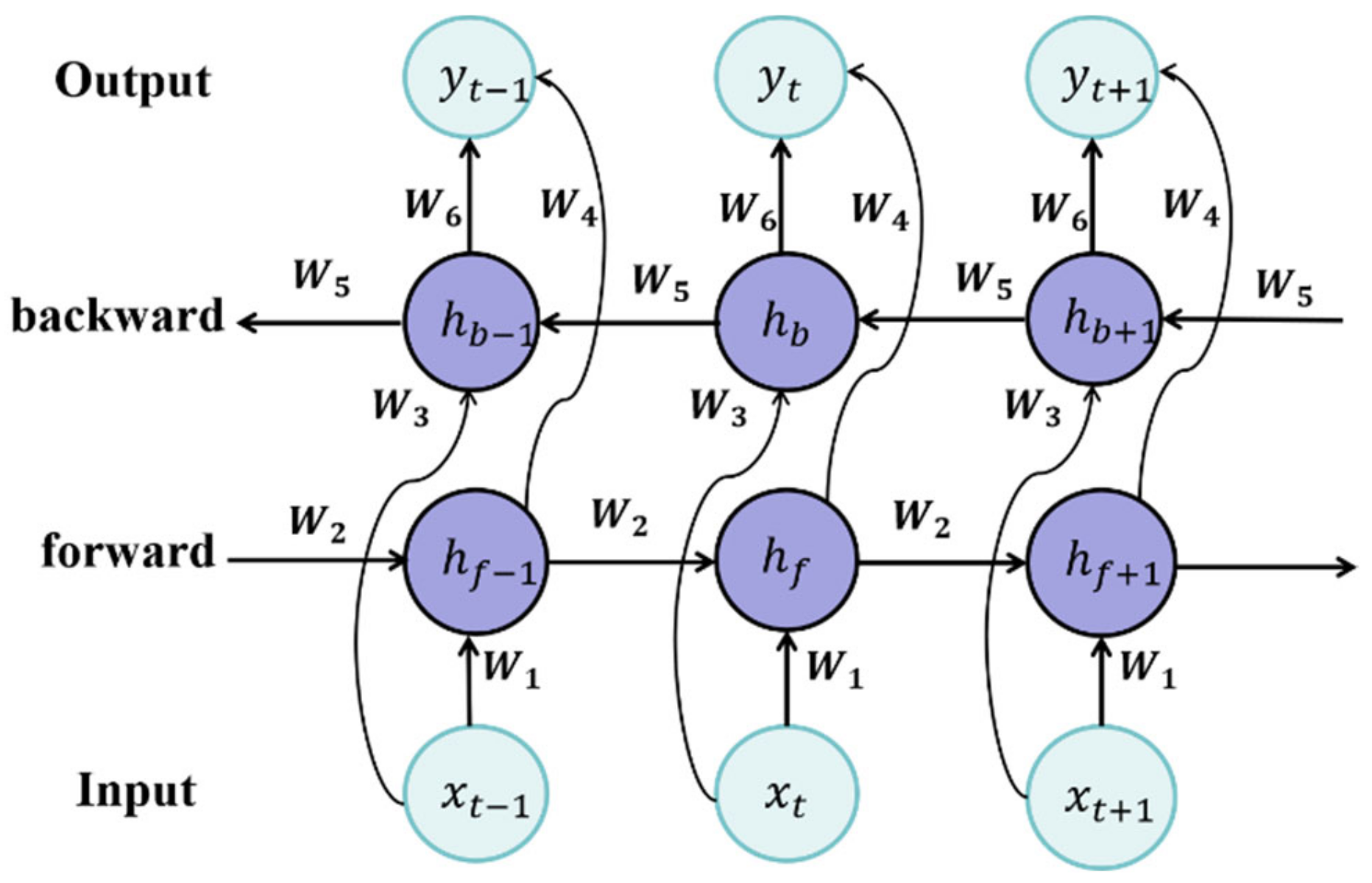
The internal structure of the BiLSTM is illustrated in Figure 2. The output, hf, was calculated for each time step, ti(i=1,2,...,n), from the forward layer, and the output, hf, was calculated using Equation (4). The backward calculation was performed in the backward layer, and the output, hb, was calculated using Equation (5); then, the final output, yt, of the BiLSTM was obtained by connecting the outputs of the forward and backward layers, which is calculated as in Equation (6).
h f = f w 1 x t + w 2 h f 1 + b f
h b = f w 3 x t + w 5 h b + 1 + b h
y t = f w 4 h f + w 6 h b + b y
where h f 1 represents the previous time-series information, x t represents the input at the current time, h b + 1 represents the subsequent time-series information, f(·) is the activation function, wi(i =1,2,3,4,5,6) is the weight between each input and output, and b represents the bias term.

2.3. Attention Mechanism

The attention mechanism was first proposed for application in the image field and was inspired by the human visual system. Now, the attention mechanism has wide-ranging applications in the network structure [37]. The attention mechanism focuses on different important regions by assigning different weights to different features in different time steps. In this study, the attention layer was a weighted summation of the BiLSTM output vectors, which was calculated as follows. The attention mechanism contents were of three parts: queries, keys, and values. The output was based on the similarity of queries and keys, and the queries with dimension, dk, were obtained by embedding a linear transformation of X on a set of inputs of dimension, dmodel [38]:
Q s = W s q X
K s = W s k X
V s = W s v X
First, the similarity between queries and keys was calculated; the resulting weights were then normalized using the softmax function, and finally, the attention value was obtained by weighting and summing it with the corresponding value. The calculation was as follows:
S i m i l a r i t y Q u e r y , K e y i = Q u e r y · K e y i Q u e r y · K e y i
A t t e n t i o n Q , K i , V = s o f t m a x Q · K i T d k V
After the input signal of the tool passes through the CNN-BiLSTM network, the information of its different life stages had different effects on the state of the neuron at the current moment. Therefore, an attention mechanism was introduced to assign different weights to the outputs of different channels of the network according to their contributions to improving the accuracy of the prediction results.

3. Proposed Methodology

3.1. Framework

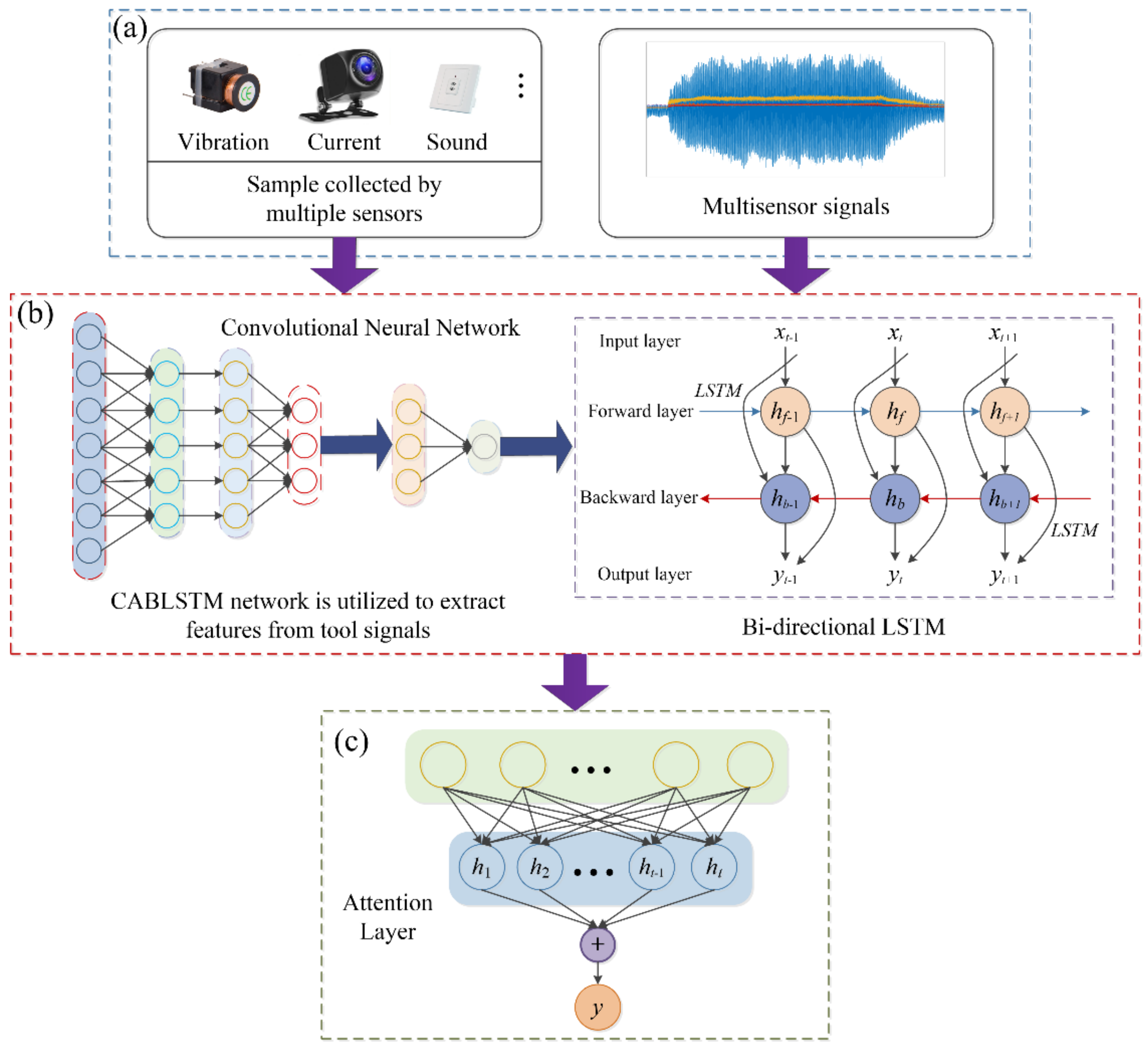
In this study, we propose a prediction method based on CNN-BiLSTM with an attention mechanism, and the flowchart of the proposed CABLSTM-predicting algorithm is shown in Figure 3, which can be generally divided into two parts: offline training and online prediction [1,37,39]. During offline training, multidimensional signals are collected for different tool wear, and the raw signal data were preprocessed with wavelet noise reduction, normalization, etc. The monitoring data with the corresponding wear quantities were constructed as the training data and used as the input to the CABLSTM network model. The structure of the CNN autonomously extracted tool degradation features, the BiLSTM extracted temporal information from the data, and the attention mechanism focused on important degradation feature information. The network allows for the autonomous and effective extraction of tool degradation features and RUL prediction.In online tool RUL prediction, for a new tool to be tested in cutting conditions, the same multidimensional signals are collected by multiple sensors as in offline training, pre-processed with the same data, and input into the trained model to predict the tool RUL online in real time.

3.2. Tool RUL Prediction Based on CABLSTM

The detailed steps of the CABLSTM structure areshown in Figure 4. (a) In the training part of the model, the data was prepared. For the signals collected by multiple sensors, invalid samples were eliminated, available data were selected, and pre-processing, such as denoising and normalization, was performed on the data. The sample time series of set length was intercepted as the training sample sequences, corresponding wear values were obtained as training labels, which with training samples were constructed as training data. (b) In the model building part, CNN can extract deep information in the tool time series through its powerful data mining and feature mapping capabilities and autonomously extract minor degradation features of the multi-dimensional sensor signals of the tool. BiLSTM can extract more comprehensive feature information by learning information from past and future moments and obtain the output of each time step, solving problems, such as long-term dependence of time series and gradient explosion. (c) The attention layer can perform further information screening on features, assign different weights to intermediate features that have a significant impact on the predicted outcome, selectively learn features from the model-training process, filter useless information, and selectively learn key information, which can improve the accuracy of the model prediction. The fullyconnected layer can reduce the dimensionality of the data and map the information to the predicted values, thereby completing the process of autonomous extraction of features to the prediction of wear values. Finally, the test sample data was constructed and fed into the trained network model to achieve wear value prediction for the target tool.
According to the ISO3685-1977 standard, the tool wear was defined as the flank wear width VB [40]. Additionally, according to the relevant literature, the tool RUL was considered terminated when the rear face wear value, VB, of the toolexceeds VBmax = 0.45 mm. Therefore, this study used the CABLSTM model to predict the current wear value, VB, of the tool, and then, the remaining useful life state parameter RUL of the tool was calculated using Equation (12)
R U L = V B m a x V B V B m a x
where RUL is the remaining useful life of the tool, VB is the rear face wear of the tool, and VBmax is the maximum rear face wear at the end of the tool life.

3.3. The Training Process of the CABLSTM Network

The training process of the CABLSTM network is summarized in Algorithm 1.
Algorithm 1 The training process of the CABLSTM network for RUL estimation.
Input: The label VB     R 1 × N .
The preprocessed monitoring signal sample, x = {xi ∈ RN×M, i = 1,…, K}, where i denotes the index of the cutter contained in the training dataset, N is the number of samples for cutter i, and M is the number of signal channels.
Output: Trained CABLSTM network.
Initialize: CNN layer parameters, LSTM layer parameters, and attention layer parameters.
Repeat
Do
Firstly, CNN is applied on the training dataset; then,the BiLSTM network is added on the top of CNN and convolved with attention layer to learn more comprehensive features.
End
The dropout layer isemployed to avoid overfitting.
Dense layers and linear regression layers are used for RUL estimation.
The ReLu function is introduced to normalize the output.
Compute the loss with the loss function MSE.
Parameters adjust:
Compute the error gradient using Adam and update network parameters.
Use the trained CABLSTM to estimate the RUL on the testing datasets.

4. Experiment

To verify the effectiveness and superiority of the proposed CABLSTM method for tool-wear-condition monitoring and remaining useful life prediction, this study explores two case studies, including (1) Milling Dataset Provided by UC Berkeley [41] and (2) IEEE PHM Challenge 2010 dataset [42]. In the first case study, the monitoring signal during tool milling was used to predict the remaining useful life of the tool. The training samples and the network construction process were also analyzed in detail. The prediction results were compared with those of six state-of-the-art prognostic methods. In the second case study, the proposed method was further validated using the tool vibration signals.
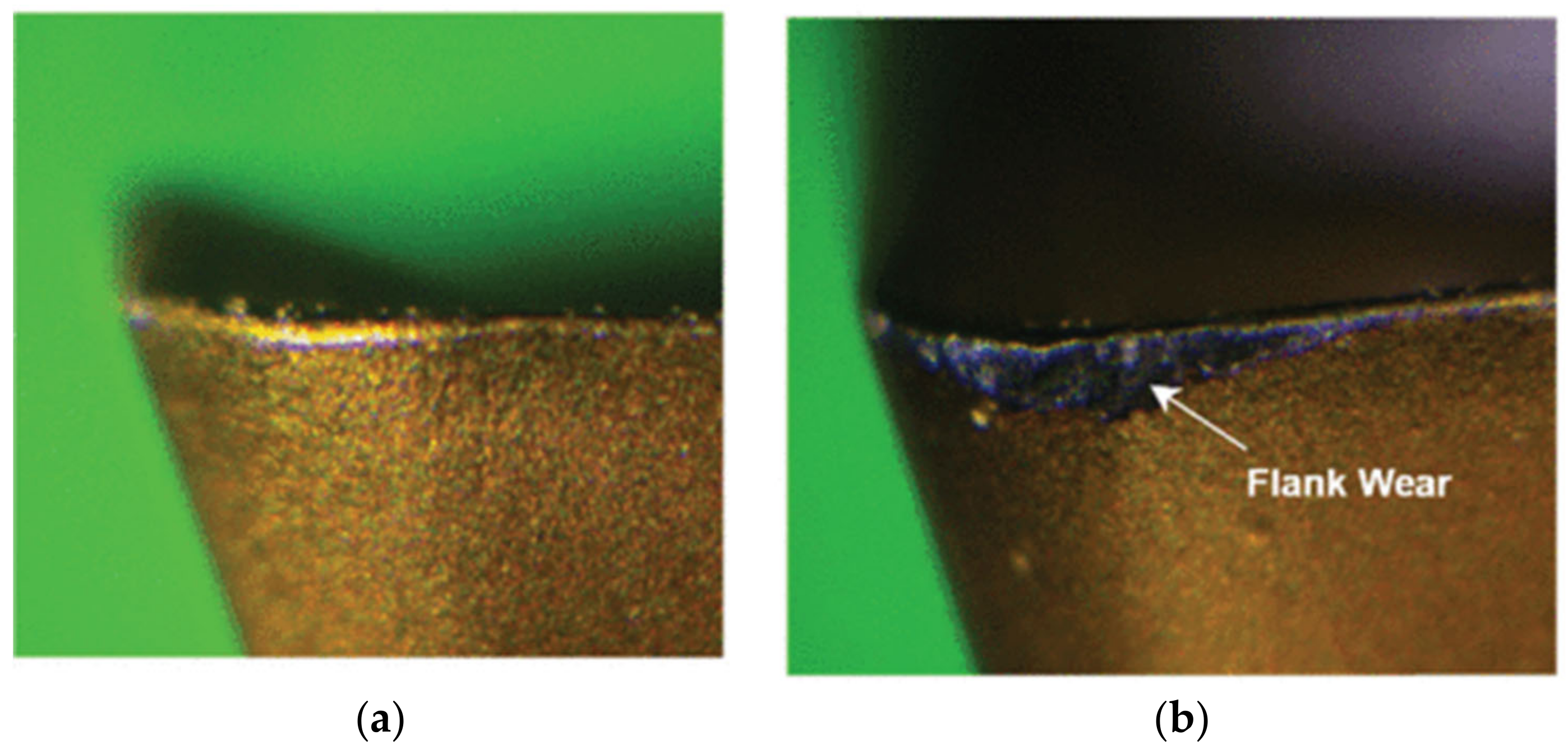
Generally, tool wear includes two forms: flank wear(VB) and crater wear(KB) [43].Currently, most researchers focus on flank wear monitoring in studies on the prediction of tool RUL, as flank wear is an influential factor in the quality, reliability, and dimensional accuracy of workpiece machining [44]. Figure 5 shows an unworn insert and a worn-out cutting worn insert. In this experiment, the flank wear VB was applied as a generallyaccepted parameter for tool wear estimate.

4.1. Case 1: Milling Dataset Provided by UC Berkeley

4.1.1. Dataset Description

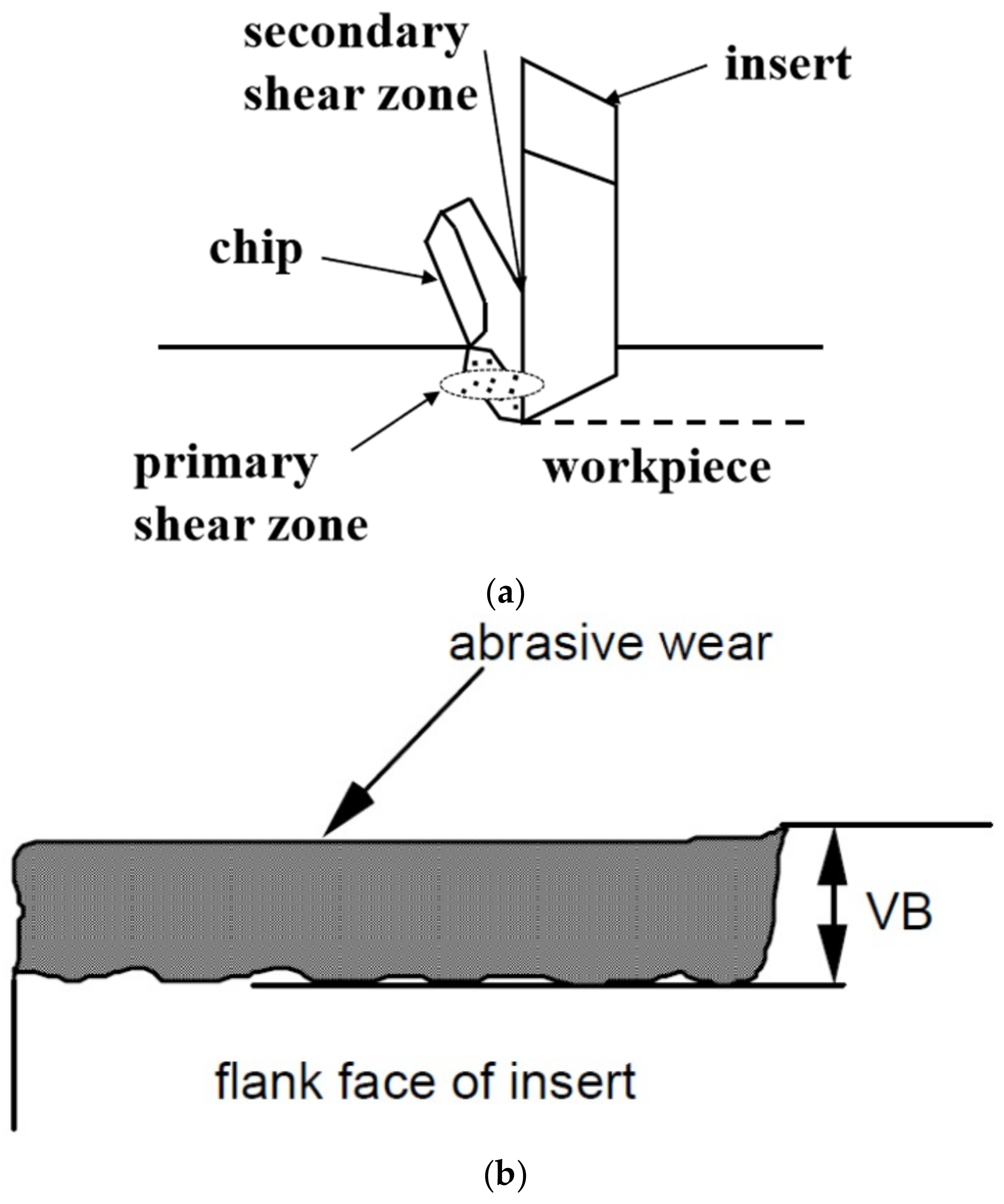
To verify the performance of the proposed approach, the Milling Dataset Provided by UC Berkeley and NASA Ames Research Center was used in this study, and the details are provided in [41]. This public data test platform is a Matsuura vertical machining center (MC-510V) milling two materials, cast iron and stainless steel, at a spindle speed of 826 rpm; the tool workpiece contact and tool wear areshown in Figure 6. The flank wear VB was measured as the distance between the cutting edge and the end of the abrasive wear on the tool flank face. At the end of each experiment the insert was removed, and the wear was measured using a microscope.

4.1.2. Experiment Parameter Setting

The experiment consisted of four cutting conditions, cut depths of 1.5 and 0.75 mm and feed rates of 0.5 and 0.25 mm/rev, and the experiment was repeated twice for each of the two materials with the cutting parameters set as listed in Table 1.
The tool used for milling was a six-tooth milling cutter (KC710), which was machined, and the wear on the rear face of the tool was measured using a microscope after each run. Data were collected for eight different working conditions, providing a data set of 16 test tool examples, containing a total of 167 run samples. As tool 6 was only run once, the data from that run was not considered.

4.1.3. Sample Data Preprocessing

The amount of signal data collected during actual monitoring and the susceptibility of the acquisition process to environmental influences requires data pre-processing. As the average life cycle is shorter when testing with stainless steel than with cast iron, it is required to predict the tool life using two different life prediction models depending on the material [46,47]. Figure 7 shows a visual image of the six sensor acquisition signals(AC spindle motor current, DC spindle motor current, RMS of vibration at spindle and table, RMS of acoustic emission at spindle and table) for tool 1 (17 runs). As shown in the figure, each run of the tool involves the processes of tool entry and exit; the process is not meant for monitoring the life conditions of the tool, and there are distinct unstable regions in the process. Therefore, in this study, only the intermediate stable regions during each run from 3000 to 7000 (containing 4000 values) of the acquired signals were used to train the CABLSTM model.
As shown in Figure 7, the signal data of the collected six−channel sensor has considerable random noise, data redundancy, etc. Therefore, it is required to perform data pre-processing on the six−channel signal, and this study adopts the wavelet denoising method, which can inhibit noise, improve the smoothness of the data, and has a high calculation speed, which is favorable for improving the prediction accuracy of the tool wear state and for denoising the acquired signals. Because of the large differences in the magnitude of the six signals that will have an impact on the prediction results, it is required to normalize the signal after noise reduction, and the calculation formula is as follows.
x ¯ i = x i μ i σ i
where μi is the mean value of the ith feature signal and xi, and σi is the standard deviation of the ith feature signal, xi.
The raw data was processed through invalid sample rejection, denoising, and normalization to achieve a uniform scale of 158 samples with a sample feature dimension of 4000 × 6. The pre-processed samples were used as the input to train the prediction model, which can accelerate the gradient descent of the prediction model and improve its accuracy.

4.1.4. Label Data Preprocessing

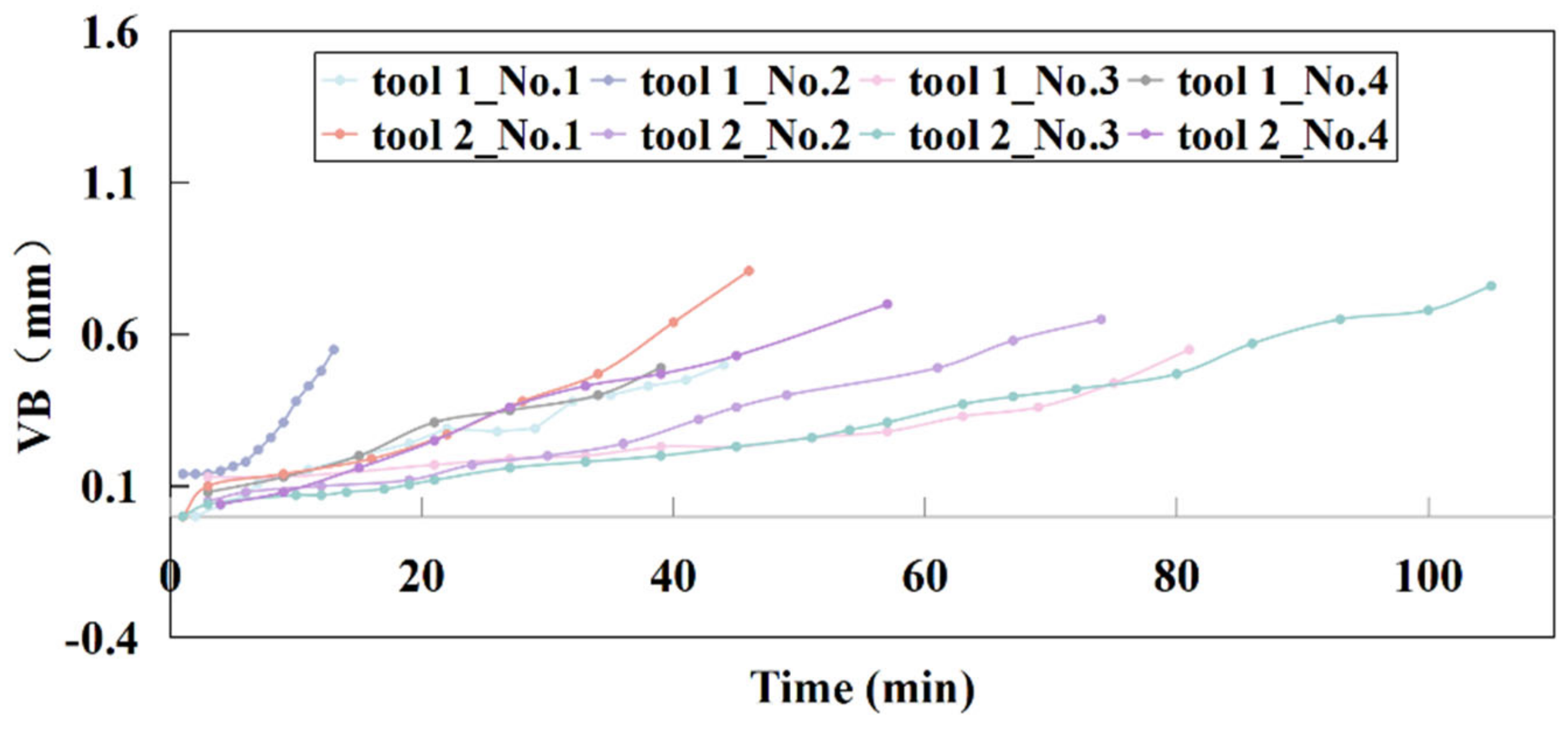
The wear measured after each run was used as a label, and as there were missing cases of wear for a few samples, linear interpolation was used to fill in the missing part of the sample wear for the 15 tools, as shown in Figure 8.

4.1.5. Model Parameter Optimization

Analyzing the conditions of the data acquired from the experiments, the average run life period of the workpiece in the tests using cast iron material is considerably higher than when steel material is used; thus, it is required to conduct separate material-specific prediction models according to the material type [48], and in this study, we selected the test data of cast iron material under four working conditions for establishing the prognostic model. Because there were only eight runs, which is considerably small, in the cast iron material tests, we used the leave-one-out method [49] for model training and validation, and the training process was to select one sample from each of the eight cast iron tool samples for prediction and the remaining seven cast iron samples for training. The current signal, vibration signal, and sound signal of the tool in its whole life cycle were made into a training sample.
The input data of the CABLSTM network were training samples and wear values, and the training samples were learned via convolutional, pooling, bidirectional LSTM, attention, and fully connected layers. The method used tool wear samples under different working conditions to train the model and validate the migration and generalization ability of the method.
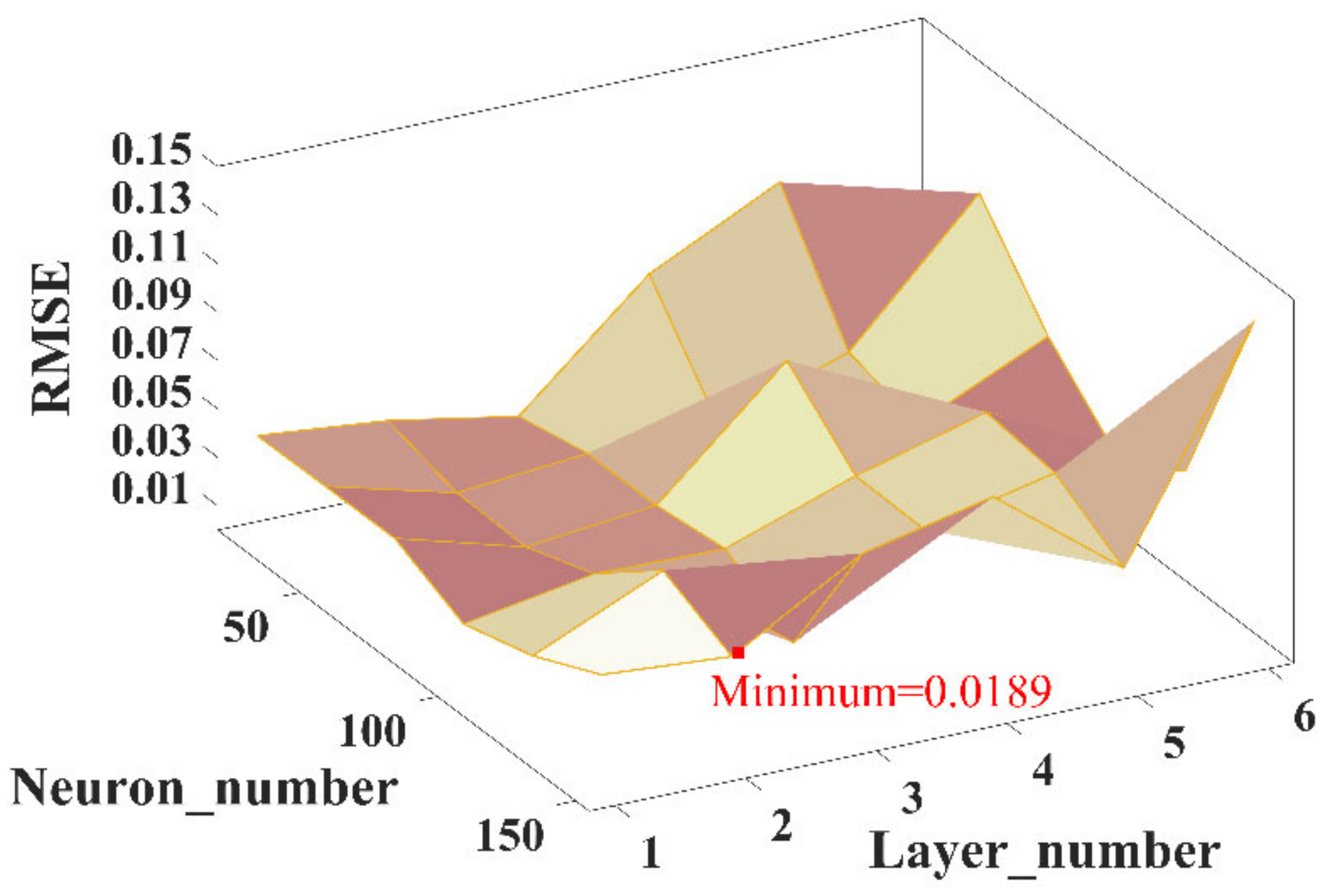
Determining the parameters of the CABLSTM model is crucial for constructing the prognostic model of the milling cutter. Therefore, the model parameters, such as the number of neurons, number of network layers, and dropout rate, should be accurately determined. In this study, we defined the number of network layers as 1–6, and the number of neurons per layer of the network was set at 50–300. The training results of the model with different layers of the network and number of neurons were calculated, as shown in Figure 9, to obtain the optimal parameters of the model, which has the smallest root mean squared error (RMSE) when the number of neurons per layer is 250 and the number of network layers is 3.
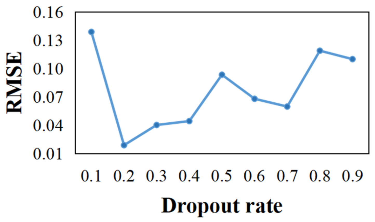
Figure 10 shows the training results of the CABLSTM model for dropout rates from 0.1 to 0.9. The model has the best training performance when the dropout rate is 0.2.
The optimal CABLSTM model for tool wear value prediction can be obtained after training, and its parameters are listed in Table 2.

4.1.6. Evaluation Indicators

To better evaluate the results of life prediction, the mean absolute error (MAE), mean absolute percentage error (MAPE), and root mean square error (RMSE) were used in this study [50,51] for quantifying the prediction results of the model, and the equation is as follows.
M A E = 1 n i = 1 n y ¯ i y i
M A P E = 100 % n i = 1 n y ¯ i y i y i
R M S E = 1 n i = 1 n y ¯ i y i 2
where yi is the true tool wear value, and y ¯ i is the tool wear predicted value.

4.1.7. Results and Discussion

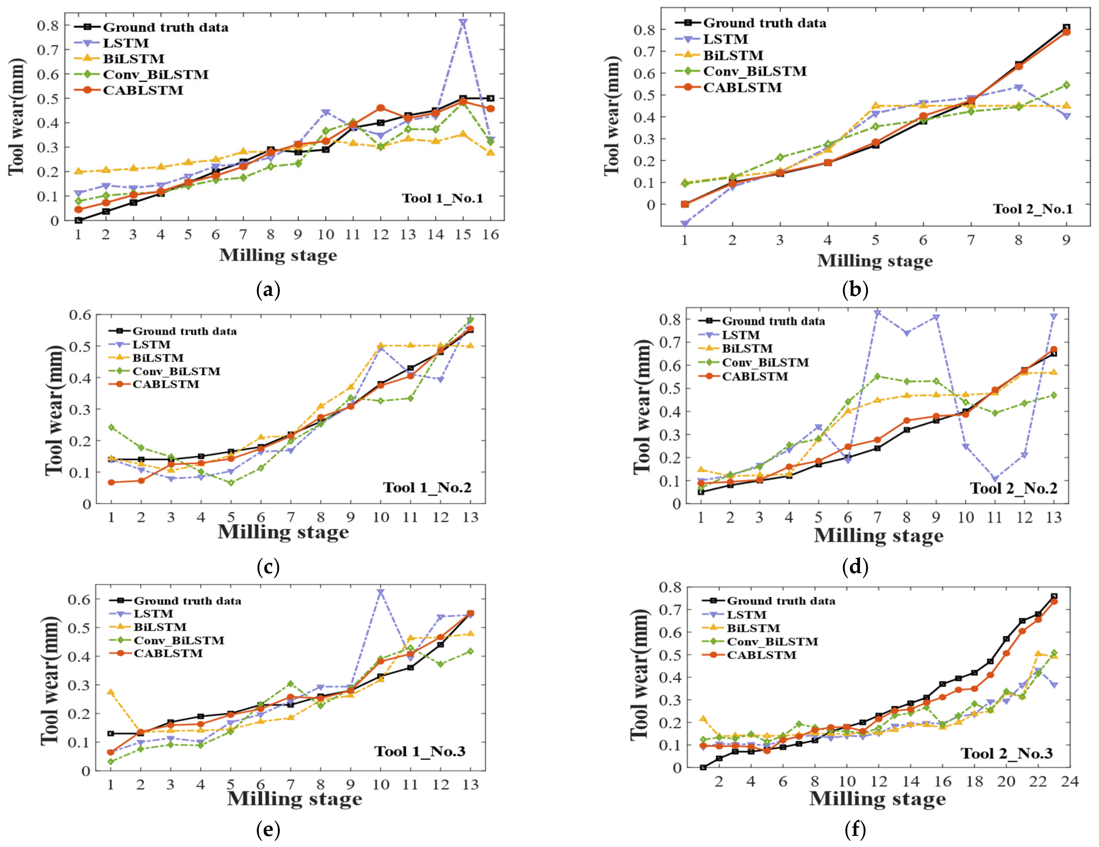
The prediction results for the full life cycle of the eight tool samples under four operating conditions, respectively, are shown in Figure 11, where the real wear values of the tool VB and the predicted wear values of the CABLSTM, LSTM, BiLSTM, and Conv_BiLSTM models are provided. As shown in the tool wear prediction effect graph, the predicted tool wear values obtained using the CABLSTM model are compared with other traditional deep-learning models, and the proposed network model achieves the highest prediction accuracy. The model can more accurately predict the tool wear value for different working conditions, which demonstrates that the proposed method has superior robustness and validates the migration and generalization ability of the method.
Using the tool wear values predicted by the above model to calculate its RUL, as shown in Figure 12, the tool life is considered terminated when RUL reaches 0 for the first two tool samples(Figure 12a,b). In the early stage of tool operation, the data input into the prediction model contains less information; thus, the prediction error is higher, whereas the more the tool is utilized in the later stage with more data input into the model, the model results are increasingly accurate. Figure 12 also shows a comparison between the RUL predicted by the proposed method and the Conv_BiLSTM method, and compared with the Conv_BiLSTM method, the CABLSTM method achieves an excellent prediction performance, and the predicted RUL is closer to the real RUL values.
To illustrate the superiority of the RUL prediction method proposed in this study, the experimental results of some methods published in recent years on the milling dataset are listed in Table 3.
Figure 11 and Figure 12 show that the RUL prediction errors of LSTM, BiLSTM, and Conv_BiLSTM are higher than CABLSTM. In addition,Table 3 shows that the CABLSTM method is superior to the other methods in terms of the three performance indicators. It is well known that the output of neurons in RNN may directly influence itself in the following period, namely “gradient disappearance” [55]. Additionally, LSTM can neither encode the information from the back to the front nor use the future information [56]. The BiLSTM network often has too many degrees of freedom, which will result in overfitting. Therefore, these methods are not suited for tool RUL prediction. The proposed CABLSTM can reduce the dimensionality of the primal sequence data by extracting the input temporal information through CNN. Due to capturing the dependencies information of both the previous and current moments, the BiLSTM network is used in CABLSTM to process time-series data. In addition,the application of the attention mechanism improves prediction accuracy because the features with different weights are considered comprehensively in different time steps. Consequently, the proposed CABLSTM can solve the above problems and improve the accuracy of tool RUL prediction.

4.2. Case 2: IEEE PHM Challenge 2010 Dataset

4.2.1. Description of Dataset

To further validate the performance of the proposed method, the PHM-2010 challenge milling dataset [42] was tested; the tool geometry is shown in Figure 13, and the experimental setup is shown in Table 4. Seven channels of signals were collected,including three-dimensional cutting forces in the X, Y, and Z-axes collected using a three-way force gauge, three-dimensional vibration signals collected using an accelerometer, and acoustic emission (AE)-RMS signals collected using an AE sensor. The tool side wear values, VB, were measured after each run.

4.2.2. Analysis and Results

The complete life data of the three tools, C1, C4, and C6, were measured in the experiments. In this study, we used these three samples of data to verify the effectiveness of the CABLSTM method for tool wear estimation. We used C4 and C6 as the training set and C1 as the test set.
For each sample, seven channels of the original monitoring signals were employed, and the same data pre-processing as in Case 1 were used to intercept the stable signals from 3000 to 215,000 for training, and the 212,000 points obtained from the interception were downsampled so that 2120 values were obtained for each sampling point as the training samples for the model with the sample format (2120.7). All three tool samples were processed as mentioned earlier and then input into the model for training.
Unlike the data in Case 1, the wear values, in this case, have a larger amount of data; thus, linear interpolation is not used for processing. The wear values at the end of each run of the tool were measured thrice in the experiment, and the largest of these wear values was used as the label for the training model in this study.
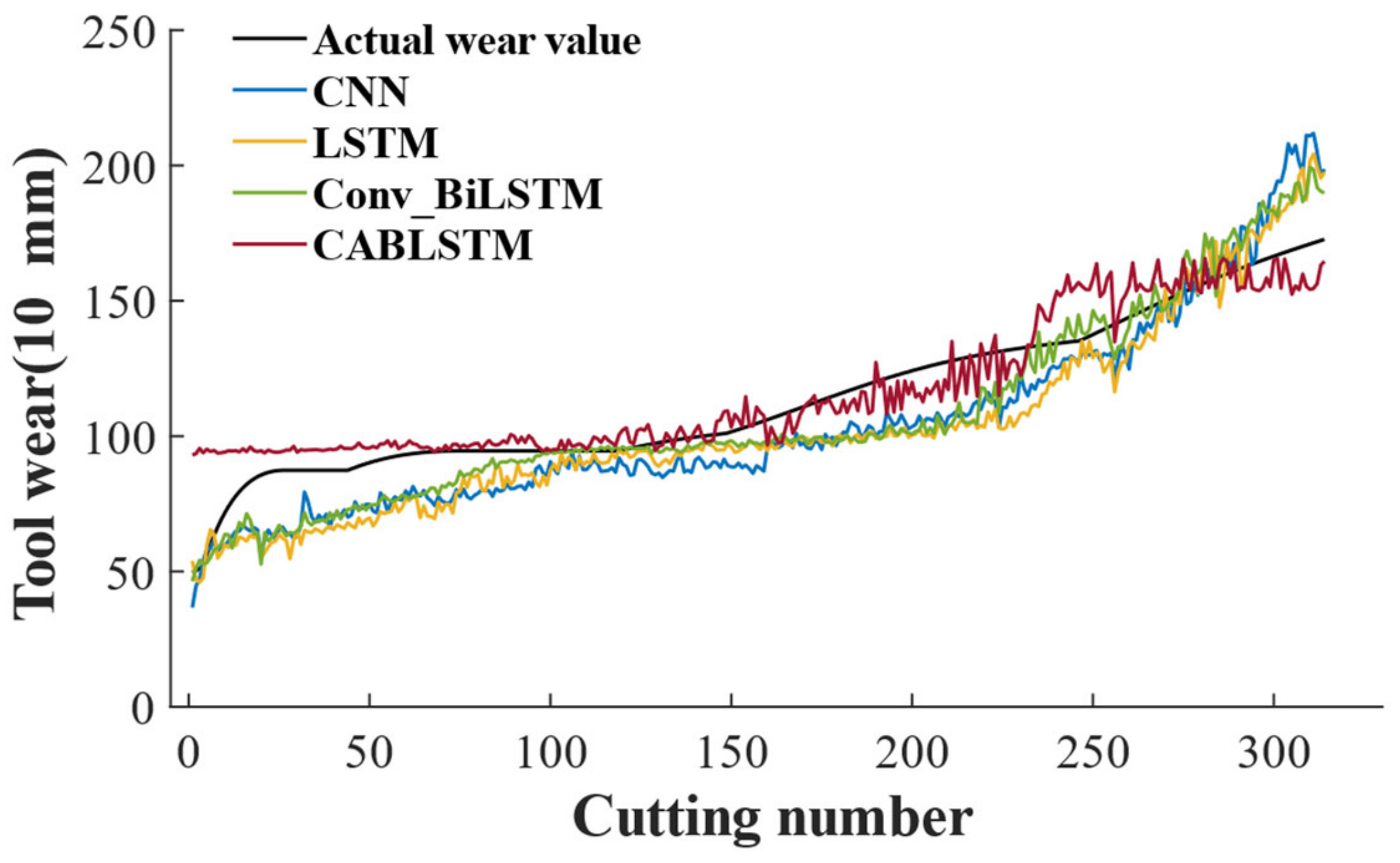
To verify the effectiveness of different methods, CABLSTM was compared with CNN, LSTM, and other methods. MAE, MAPE, and RMSE were adopted to quantify the estimation performances of these methods. Figure 14 shows the tool wear estimation results of C1 from which it can be seen that the proposed method achieves superior prediction results.
The errors between the predicted and actual values of tool wear are listed in Table 5. The prediction results with the four methods on tool C1 were compared, and the prediction accuracy of the proposed method exceeds those of the other two methods. However, because of the small number of available training samples, the prediction performance of the model is unfavorable compared with Case 1; this can be improved by increasing the number of training samples.

5. Conclusions

In this study, we proposed an RUL prediction method based on the CNN-BiLSTM network and attention mechanism. Tool wear monitoring and RUL prediction under multiple working conditions were achieved. The main conclusions of this study are as follows:
  • The CABLSTM model-based RUL prediction method directly applies sensor monitoring data and achieves tool wear monitoring and RUL prediction after data pre-processing, using the model to adaptively extract features for autonomous learning, overcoming the limitations and complexity of manual feature extraction, and simplifying the traditional RUL prediction process.
  • In this study, the attention mechanism was incorporated into the CNN-BiLSTM network, which can selectively learn the features in the training process of the model, mine the hidden information in the data, and accurately predict the tool RUL.
  • The validity of the method was verified using two datasets, and the CABLSTM model obtains better prediction error indicators compared with traditional RNN, CNN, LSTM, BiLSTM, etc. The method proposed in this study predicts the best results and demonstrates that the proposed model has better performance for the RUL prediction. Meanwhile, the model was applied to the tool data under different working conditions, which validated the migration and generalization ability of the method.

Author Contributions

Conceptualization, L.N. and L.Z.; methodology, L.N. and L.Z.; software, L.Z.; validation, L.Z. and S.X.; formal analysis, W.C.; investigation, L.Z. and H.Y.; resources, L.N.; data curation, L.Z.; writing—original draft preparation, L.Z.; writing—review and editing, L.Z. and H.Y.; visualization, S.X. All authors have read and agreed to the published version of the manuscript.

Funding

This research was funded by the National Natural Science Foundation of China (Grant No. 51975191.).

Data Availability Statement

The data used to support the findings of this study are available fromthe corresponding author upon reasonable request. The main code used for the tool RUL prediction are openly available at https://gitee.com/zhang-lvfan/dl, accessed on 5 October 2022.

Acknowledgments

The support is gratefully acknowledged. The authors would also like to thank the reviewers for their valuable suggestions and comments.

Conflicts of Interest

The authors declare no conflict of interest.

References

  1. Gao, C.; Bintao, S.; Wu, H.; Peng, M.; Zhou, Y. New Tool Wear Estimation Method of the Milling Process Based on Multisensor Blind Source Separation. Math. Probl. Eng. 2021, 2021, 11. [Google Scholar] [CrossRef]
  2. Feng, T.; Guo, L.; Gao, H.; Chen, T.; Yu, Y.; Li, C. A new time-space attention mechanism driven multi-feature fusion method for tool wear monitoring. Int. J. Adv. Manuf. Technol. 2022, 120, 5633–5648. [Google Scholar] [CrossRef]
  3. Zhang, X.; Han, C.; Luo, M.; Zhang, D. Tool Wear Monitoring for Complex Part Milling Based on Deep Learning. Appl. Sci. 2020, 10, 6916. [Google Scholar] [CrossRef]
  4. Yaguo, L.; Naipeng, L.; Szymon, G.; Jing, L.; Stanislaw, R.; Jacek, D. A Model-Based Method for Remaining Useful Life Prediction of Machinery. IEEE Trans. Reliab. 2016, 65, 1314–1326. [Google Scholar] [CrossRef]
  5. Juan, C.; María, L.J.; Manuel, C.; Athanasios, K. A Markov chains prognostics framework for complex degradation processes. Reliab. Eng. Syst. Saf. 2020, 195, 106621. [Google Scholar] [CrossRef]
  6. Hongyan, D.; Shubin, S.; Ming, J.Z.; Shudong, S. Semi-Markov Process-Based Integrated Importance Measure for Multi-State Systems. IEEE Trans. Reliab. 2015, 64, 754–765. [Google Scholar] [CrossRef]
  7. Xiao-Sheng, S.; Wenbin, W.; Mao-Yin, C.; Chang-Hua, H.; Dong-Hua, Z. A degradation path-dependent approach for remaining useful life estimation with an exact and closed-form solution. Eur. J. Oper. Res. 2013, 226, 53–66. [Google Scholar] [CrossRef]
  8. Han, W.; Xiaobing, M.; Yu, Z. An improved Wiener process model with adaptive drift and diffusion for online remaining useful life prediction. Mech. Syst. Signal Pr. 2019, 127, 370–387. [Google Scholar] [CrossRef]
  9. Sun, H.; Cao, D.; Zhao, Z.; Kang, X. A Hybrid Approach to Cutting Tool Remaining Useful Life Prediction Based on the Wiener Process. IEEE T. Reliab. 2018, 67, 1294–1303. [Google Scholar] [CrossRef]
  10. Jianbo, Y. Health Degradation Detection and Monitoring of Lithium-Ion Battery Based on Adaptive Learning Method. IEEE Trans. Instrum. Meas. 2014, 63, 1709–1721. [Google Scholar] [CrossRef]
  11. Lucas, E.; Christophe, L.; Roger, S.; Pierre, D. Estimate of Cutting Tool Lifespan through Cox Proportional Hazards Model. IFAC Pap. 2016, 49, 238–243. [Google Scholar] [CrossRef]
  12. Huibin, S.; Junlin, P.; Jiduo, Z.; Dali, C. Non-linear Wiener process–based cutting tool remaining useful life prediction considering measurement variability. Int. J. Adv. Manuf. Technol. 2020, 107, 4493–4502. [Google Scholar] [CrossRef]
  13. Naipeng, L.; Yaguo, L.; Tao, Y.; Ningbo, L.; Tianyu, H. A Wiener-Process-Model-Based Method for Remaining Useful Life Prediction Considering Unit-to-Unit Variability. IEEE Trans. Ind. Electron. 2019, 66, 2092–2101. [Google Scholar] [CrossRef]
  14. Wang, C.; Jiang, W.; Yue, Y.; Zhang, S. Research on Prediction Method of Gear Pump Remaining Useful Life Based on DCAE and Bi-LSTM. Symmetry 2022, 14, 1111. [Google Scholar] [CrossRef]
  15. Paulo, R.D.O.D.; Alp, A.; Yingqian, Z.; Uzay, K. Remaining useful lifetime prediction via deep domain adaptation. Reliab. Eng. Syst. Saf. 2020, 195, 106682. [Google Scholar] [CrossRef] [Green Version]
  16. Chaochao, C.; Bin, Z.; George, V. Prediction of Machine Health Condition Using Neuro-Fuzzy and Bayesian Algorithms. IEEE T. Instrum. Meas. 2012, 61, 297–306. [Google Scholar] [CrossRef]
  17. Benkedjouh, T.; Medjaher, K.; Zerhouni, N.; Rechak, S. Health assessment and life prediction of cutting tools based on support vector regression. J. Intell. Manuf. 2015, 26, 213–223. [Google Scholar] [CrossRef] [Green Version]
  18. Vakharia, V.; Pandya, S.; Patel, P. Tool wear rate prediction using discrete wavelet transform and K-Star algorithm. Life Cycle Reliab. Saf. Eng. 2018, 7, 115–125. [Google Scholar] [CrossRef]
  19. Zang, C.; Imregun, M. Combined neural network and reduced FRF techniques for slight damage detection using measured response data. Arch. Appl. Mech. (Ing. Arch.) 2001, 71, 525–536. [Google Scholar] [CrossRef]
  20. Bin, Z.; Chris, S.; Carl, S.B.; Romano, P.; Marcos, E.O.; George, J.V. A Probabilistic Fault Detection Approach: Application to Bearing Fault Detection. IEEE Trans. Ind. Electron. 2011, 58, 2011–2018. [Google Scholar] [CrossRef]
  21. Chen, J.; Chen, D.; Liu, G. Using temporal convolution network for remaining useful lifetime prediction. Eng. Rep. 2020, 3, e12305. [Google Scholar] [CrossRef]
  22. Sun, H.; Zhang, J.; Mo, R.; Zhang, X. In-process tool condition forecasting based on a deep learning method. Robot. Cim.Int. Manuf. 2020, 64, 101924. [Google Scholar] [CrossRef]
  23. Yaguo, L.; Naipeng, L.; Liang, G.; Ningbo, L.; Tao, Y.; Jing, L. Machinery health prognostics: A systematic review from data acquisition to RUL prediction. Mech. Syst. Signal Pr. 2018, 104, 799–834. [Google Scholar] [CrossRef]
  24. Yu, W.; Kim, I.Y.; Mechefske, C. Remaining useful life estimation using a bidirectional recurrent neural network based autoencoder scheme. Mech. Syst. Signal Pr. 2019, 129, 764–780. [Google Scholar] [CrossRef]
  25. Guisheng, H.; Shuo, X.; Nan, Z.; Lei, Y.; Quanhao, F.; Anastasios, D.D. Remaining Useful Life Estimation Using Deep Convolutional Generative Adversarial Networks Based on an Autoencoder Scheme. Comput. Intell. Neurosci. 2020, 2020, 1–14. [Google Scholar] [CrossRef]
  26. Xincheng, C.; Binqiang, C.; Bin, Y.; Shiqiang, Z. An Intelligent Milling Tool Wear Monitoring Methodology Based on Convolutional Neural Network with Derived Wavelet Frames Coefficient. Appl. Sci. 2019, 9, 3912. [Google Scholar] [CrossRef] [Green Version]
  27. Huang, Z.; Zhu, J.; Lei, J.; Li, X.; Tian, F. Tool Wear Monitoring with Vibration Signals Based on Short-Time Fourier Transform and Deep Convolutional Neural Network in Milling. Math. Probl. Eng. 2021, 2021, 1–14. [Google Scholar] [CrossRef]
  28. Marei, M.; Li, W. Cutting tool prognostics enabled by hybrid CNN-LSTM with transfer learning. Int. J. Adv. Manuf. Technol. 2021, 118, 817–836. [Google Scholar] [CrossRef]
  29. Rui, Z.; Ruqiang, Y.; Jinjiang, W.; Kezhi, M. Learning to Monitor Machine Health with Convolutional Bi-Directional LSTM Networks. Sensors 2017, 17, 273. [Google Scholar] [CrossRef] [Green Version]
  30. Jiahang, L.; Xu, Z. Convolutional neural network based on attention mechanism and Bi-LSTM for bearing remaining life prediction. Appl. Intell. 2021, 52, 1076–1091. [Google Scholar] [CrossRef]
  31. Karpathy, A.; Fei-Fei, L. Deep Visual-Semantic Alignments for Generating Image Descriptions. IEEE T. Pattern Anal. 2017, 39, 664–676. [Google Scholar] [CrossRef] [PubMed] [Green Version]
  32. Gang, L.; Jiabao, G. Bidirectional LSTM with attention mechanism and convolutional layer for text classification. Neurocomputing 2019, 337, 325–338. [Google Scholar] [CrossRef]
  33. Wang, B.; Lei, Y.; Li, N.; Wang, W. Multiscale Convolutional Attention Network for Predicting Remaining Useful Life of Machinery. IEEE T. Ind. Electron. 2021, 68, 7496–7504. [Google Scholar] [CrossRef]
  34. Zhiwen, H.; Jianmin, Z.; Jingtao, L.; Xiaoru, L.; Fengqing, T. Tool wear predicting based on multi-domain feature fusion by deep convolutional neural network in milling operations. J. Intell. Manuf. 2019, 31, 953–966. [Google Scholar] [CrossRef]
  35. Cheng, M.; Jiao, L.; Yan, P.; Jiang, H.; Wang, R.; Qiu, T.; Wang, X. Intelligent tool wear monitoring and multi-step prediction based on deep learning model. J. Manuf. Syst. 2022, 62, 286–300. [Google Scholar] [CrossRef]
  36. Qinglong, A.; Zhengrui, T.; Xingwei, X.; Mohamed, E.M.; Ming, C. A data-driven model for milling tool remaining useful life prediction with convolutional and stacked LSTM network. Measurement 2020, 154, 107461. [Google Scholar] [CrossRef]
  37. Zhang, J.; Jiang, Y.; Wu, S.; Li, X.; Luo, H.; Yin, S. Prediction of remaining useful life based on bidirectional gated recurrent unit with temporal self-attention mechanism. Reliab. Eng. Syst. Safe. 2022, 221, 108297. [Google Scholar] [CrossRef]
  38. Cao, Y.; Ding, Y.; Jia, M.; Tian, R. A novel temporal convolutional network with residual self-attention mechanism for remaining useful life prediction of rolling bearings. Eng. Syst. Saf. 2021, 215, 107813. [Google Scholar] [CrossRef]
  39. Yu, W.; Shao, Y.; Xu, J.; Mechefske, C. An adaptive and generalized Wiener process model with a recursive filtering algorithm for remaining useful life estimation. Reliab. Eng. Syst. Saf. 2022, 217, 108099. [Google Scholar] [CrossRef]
  40. Zhi, G.; He, D.; Sun, W.; Zhou, Y.; Pan, X.; Gao, C. An edge-labeling graph neural network method for tool wear condition monitoring using wear image with small samples. Meas. Sci. Technol. 2021, 32, 64006. [Google Scholar] [CrossRef]
  41. Agogino, A.; Goebel, K. Mill Data Set. Berkeley, CA, USA. 2007. Available online: https://ti.arc.nasa.gov/tech/dash/groups/pcoe/prognostic-data-repository/ (accessed on 30 August 2022).
  42. PHM Society Conference Data Challenge. 2010. Available online: http://www.phmsociety.org/competition/phm/10 (accessed on 30 August 2022).
  43. Sayyad, S.; Kumar, S.; Bongale, A.; Kamat, P.; Patil, S.; Kotecha, K. Data-Driven Remaining Useful Life Estimation for Milling Process: Sensors, Algorithms, Datasets, and Future Directions. IEEE Access 2021, 9, 110255–110286. [Google Scholar] [CrossRef]
  44. Palanisamy, P.; Rajendran, I.; Shanmugasundaram, S. Prediction of tool wear using regression and ANN models in end-milling operation. Int. J. Adv. Manuf. Technol. 2008, 37, 29–41. [Google Scholar] [CrossRef]
  45. Paulino, G.N.; Esperanza, G.; Celestino, O.G.; Antonio, B.S. Hybrid ABC Optimized MARS-Based Modeling of the Milling Tool Wear from Milling Run Experimental Data. Materials 2016, 9, 82. [Google Scholar] [CrossRef] [Green Version]
  46. Usynin, A.V. A Generic Prognostic Framework for Remaining Useful Life Prediction of Complex Engineering Systems. Ph.D. Thesis, University of Tennessee, Knoxville, TN, USA, 2007. Available online: https://trace.tennessee.edu/utk_graddiss/319 (accessed on 30 August 2022).
  47. Coble, J.B. Merging Data Sources to Predict Remaining Useful Life—An Automated Method to Identify Prognostic Parameters. Ph.D. Thesis, University of Tennessee, Knoxville, TN, USA, 2010. Available online: https://trace.tennessee.edu/utk_graddiss/683 (accessed on 30 August 2022).
  48. Camci, F.; Medjaher, K.; Zerhouni, N.; Nectoux, P. Feature Evaluation for Effective Bearing Prognostics. Qual. Reliab. Eng. Int. 2013, 29, 477–486. [Google Scholar] [CrossRef] [Green Version]
  49. Songsong, Y.; Shilong, W.; Lili, Y.; Hong, X.; Yang, C.; Shouli, S. A novel monitoring method for turning tool wear based on support vector machines. Proc. Inst. Mech. Eng. Part B J. Eng. Manuf. 2016, 230, 1359–1371. [Google Scholar] [CrossRef]
  50. Duan, Y.; Li, H.; He, M.; Zhao, D. A BiGRU Autoencoder Remaining Useful Life Prediction Scheme with Attention Mechanism and Skip Connection. IEEE Sens. J. 2021, 21, 10905–10914. [Google Scholar] [CrossRef]
  51. Yuqing, Z.; Weifang, S. Tool Wear Condition Monitoring in Milling Process Based on Current Sensors. IEEE Access 2020, 8, 95491–95502. [Google Scholar] [CrossRef]
  52. Zhu, Y.; Wu, J.; Wu, J.; Liu, S. Dimensionality reduce-based for remaining useful life prediction of machining tools with multisensor fusion. Reliab. Eng. Syst. Saf. 2022, 218, 108179. [Google Scholar] [CrossRef]
  53. Xia, P.; Huang, Y.; Xiao, D.; Liu, C.; Shi, L. Tool Wear Prediction Under Varying Milling Conditions via Temporal Convolutional Network and Auxiliary Learning. In Proceedings of the 2021 IEEE International Conference on Prognostics and Health Management (ICPHM), Detroit, MI, USA, 7–9 June 2021; pp. 1–6. [Google Scholar] [CrossRef]
  54. Changfu, L.; Lida, Z. A two-stage approach for predicting the remaining useful life of tools using bidirectional long short-term memory. Measurement 2020, 164, 108029. [Google Scholar] [CrossRef]
  55. Shouxiang, W.; Xuan, W.; Shaomin, W.; Dan, W. Bi-directional long short-term memory method based on attention mechanism and rolling update for short-term load forecasting. Int. J. Electr. Power Energy Syst. 2019, 109, 479–480. [Google Scholar] [CrossRef]
  56. Jiang, J.-R.; Lee, J.-E.; Zeng, Y.-M. Time Series Multiple Channel Convolutional Neural Network with Attention-Based Long Short-Term Memory for Predicting Bearing Remaining Useful Life. Sens. Res. 2020, 1, 166. [Google Scholar] [CrossRef] [PubMed]
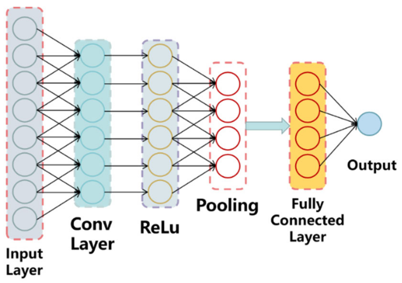
Figure 1. Convolutional neural network.
Symmetry 14 02243 g001
Figure 2. BiLSTM network.
Symmetry 14 02243 g002
Figure 3. The flowchart of the proposed CABLSTM predicting algorithm.
Symmetry 14 02243 g003
Figure 4. CABLSTM structure diagram.
Symmetry 14 02243 g004
Figure 5. Cutting tool insert: (a) unworn (b) worn tool (flank wear).
Symmetry 14 02243 g005
Figure 6. Tool workpiece contact and tool wear: (a) shear zones at tool/workpiece interface; (b) tool wear VB [45].
Symmetry 14 02243 g006
Figure 7. Sensor signal of the tool cutting number 1 with the first time.
Symmetry 14 02243 g007
Figure 8. Cast iron wear of eight cuttings.
Symmetry 14 02243 g008
Figure 9. Training result of the CABLSTM model with different layers and neuron numbers.
Symmetry 14 02243 g009
Figure 10. Training result of the CABLSTM model with different dropout rates.
Symmetry 14 02243 g010
Figure 11. On-site predicted tool wear against the observed value of eight cases: (a) four methods prediction results of the first experimental tool in cut depths of 1.5 mm, feed rates of 0.5 mm/rev; (b) four methods prediction results of the second experimental tool in depths of 1.5 mm, feed rates of 0.5 mm/rev; (c) four methods prediction results of the first experimental tool in cut depths of 0.75 mm, feed rates of 0.5 mm/rev; (d) four methods prediction results of the second experimental tool in cut depths of 0.75 mm, feed rates of 0.5 mm/rev; (e) four methods prediction results of the first experimental tool in cut depths of 0.75 mm, feed rates of 0.25 mm/rev; (f) four methods prediction results of the second experimental tool in cut depths of 0.75 mm, feed rates of 0.25 mm/rev; (g) four methods prediction results of the first experimental tool in cut depths of 1.5 mm, feed rates of 0.25 mm/rev; (h) four methods prediction results of the second experimental tool in cut depths of 1.5 mm, feed rates of 0.25 mm/rev.
Symmetry 14 02243 g011aSymmetry 14 02243 g011b
Figure 12. RUL estimations result with two models on the milling datasets: (a) tool 1; (b) tool 2.
Symmetry 14 02243 g012
Figure 13. The tool of the experimental.
Symmetry 14 02243 g013
Figure 14. Comparison of prediction results of testing tool C1.
Symmetry 14 02243 g014
Table 1. Cutting parameters set.
MaterialTool Cutting
Number
Depth of Cut
d/mm
Feed
c/(mm/rev)
Number of Runs
First TimeSecond Time
Cast iron11.50.5179
20.750.51415
30.750.251423
41.50.25710
Stainless steel J4551.50.566
61.50.2517
70.750.25815
80.750.569
Table 2. Parameters of the trained CABLSTM model.
No.ParametersValue
1Convolution layer numbers1
2BiLSTM layer numbers1
3Attention layer1
4Neurons in each layer250
5Dropout rate0.2
6Training epochs750
7Batch size32
8Loss functionMean square error
9OptimizerAdam
Table 3. RUL prediction comparison of the proposed method with other methods.
MethodologyMAERMSEMAPE
RNN0.09490.128329.72%
LSTM0.06130.095417.41%
BiLSTM0.07620.061813.61%
Zhu’s [52]-0.03143.46%
TCN [53]0.12090.1422-
CNN [54]-0.088012.2%
Conv_BiLSTM0.07890.088435.84%
CABLSTM0.02870.02318.85%
Table 4. Experimental conditions in the dataset.
Experimental ConditionsParameter
MachineRoders Tech RFM760
Workpiece materialInconel 718 (Jet engines)
Cutter3-flute ball nose
Spindle speed (r/min)10,400
Feed rate (mm/min)1555
Y depth of cut (radial)(mm)0.125
Z depth of cut (axial)(mm)0.2
Sensors5
Sensor channels7
Sampling data50KHz
Table 5. Estimation errors of five methods with testing set C1.
MethodologyMAEMAPERMSE
LSTM14.276615.77%16.3948
CNN13.804514.56%15.5764
Conv-BiLSTM11.037111.53%13.4803
SSA+LS-SVM [1]--8.4653
CABLSTM7.46886.47%8.1661
Publisher’s Note: MDPI stays neutral with regard to jurisdictional claims in published maps and institutional affiliations.