Abstract
In the paper a finite-capacity discrete-time queueing system with geometric interarrival times and generally distributed processing times is studied. Every time when the service station becomes idle it goes for a vacation of random duration that can be treated as a power-saving mechanism. Application of a single vacation policy is one way for the system to achieve symmetry in terms of system operating costs. A system of differential equations for the transient conditional queue-size distribution is established. The solution of the corresponding system written for double probability generating functions is found using the analytical method based on a linear algebraic approach. Moreover, the representation for the probability-generating function of the stationary queue-size distribution is obtained. Numerical study illustrating theoretical results is attached as well.
1. Introduction
Queueing models with a discrete-time parameter are an important alternative to the systems with continuous time which are used most often in modeling. In fact, continuous-time systems were initially proposed in the works of Erlang, a precursor of queueing theory, who assumed—in accordance with the nature of telecommunication traffic—a continuous distribution of the duration of a telephone call. Until 1958, the year of the publication of Torben Meisling’s work [1], they were almost exclusively used and analyzed in queueing theory.
The special application of discrete-time models is associated with the modeling of processing (sending) packets in the nodes of digital telecommunication and computer networks. In discrete models time is divided into fixed-length intervals (called slots), which, in fact, play the role of the smallest undivided time units. Because, as a rule, time slots are short, it is not important for practice at what moment they are affected or terminated. We will refer, for clarity, to the start of the time slot. One can find the overview of main results related to discrete-time queueing models, e.g., in [2,3,4]. One of the first numerical analyses of such models was proposed in [5].
One of the key research areas in the field of design and development of wireless communication is the issue of energy saving. In the literature, different-type approaches and solutions are proposed. One of them is the exhaustive single vacation policy in that the service station (that can be identified as a network node) is switched off for a certain period (deterministic or random) whenever the system empties (the buffer does not contain waiting jobs and the service station is idle). The cost of maintaining a server in a ready-to-process state is generally significantly higher than the cost of mere job accumulation during the non-servicing period. Of course, suspension of service involves an increase in waiting times and the subsequent risk of losing jobs due to buffer overload. In consequence, such a policy is one way for the system to achieve symmetry in terms of system operating costs. Single vacation policy can be used in the modeling of the operation of mobile network nodes (e.g. working under the IEEE 802.16e Mobile WiMAX protocol) in which sleep and active periods change cyclically. Moreover, in the automated production line, if the accumulating buffer becomes empty, machine conservation is sometimes planned that can be treated as a machine vacation.
In the paper, we study the queue-size distribution in a finite-buffer discrete-type model with a single vacation policy in the transient state. Non-stationary results for different-type queueing models are much rarer than those obtained for the steady state of the system. However, transient analysis is sometimes more desirable. For example, a system in which the traffic intensity is sparse (such a situation can be observed, e.g., in wireless sensor network node) or the traffic/processing rates change quite often, or a new control mechanism is implemented, requires rather time-dependent analysis than the stationary one. Applying the total probability law with respect to the first departure epoch after the opening of the system, we build a system of differential equations for the queue-size distribution at the fixed moment t conditioned by the buffer state at the starting time The solution of the corresponding system written for double probability generating functions (PGFs for short) is derived in a compact form with the support of a linear algebraic approach.
The overview of different-type models with service interruptions can be found in [6]. A discrete-time model described by geometric distributions operating under a multiple vacation policy was investigated in [7]. Stationary distributions of the queue size and waiting time were obtained there using quasi-birth-and-death chain and matrix-geometric solution methods. In [8] an infinite-buffer discrete-time model with multiple vacation policies was studied. By using the matrix-geometric approach stationary representations for the queue size and waiting time distributions were obtained. The same queueing system was investigated in [9] in the case of a single vacation scheme. A modification of the classical single/multiple vacation policy for the discrete-time model was considered in [10] where server vacations occur whenever the queue becomes empty or whenever a timer expires. In [11] a class of single-server discrete-time queueing models with server vacations, individual arrivals, and non-batch service was considered. It was shown that, under the assumption that interarrival, service, vacation, and server operational times can be cast with Markov-based representation, the class can be tractable as a matrix–geometric or a matrix-product problem. A -type queue with a single vacation mechanism was studied in [12]. In [13] a more general -type model was investigated. Representations for stationary distributions of the queue size at arrivals epochs and of the waiting time for an arbitrary job were found there using the matrix-geometric solution method. The supplementary variable technique was used in [14] to find main performance measures in a discrete-time model operating under multiple vacations and with setup-closedown times. Discrete-time queueing model with a single vacation policy was considered in [15]. The case of a multiple vacation policy was analyzed in [16]. The additional strategy of the N-policy was studied in [17]. One can find the solution to the problem of equilibrium strategies in discrete-time Markovian queues working under single and multiple vacations in [18]. In [19] (see also [20]) another mechanism limiting the access to the service station was considered, namely a dropping function “filtering” the arrival stream in dependence on the current queue size. An alternative strategy was studied in [21] where a flexible queueing system was analyzed that adapts to the system size by using a single or a bulk service discipline. Transient results for queueing models with vacation policies can be found e.g., in [22,23,24,25] (see also [26,27]). Moreover, one can find in [28,29,30] some new results for systems with different-type restrictions in the access to the service facility. In particular, in [28] a model with active queue management is studied.
The remaining part of the paper is organized as follows. The detailed mathematical description of the system is given in the next Section 2. The system of difference equations for the transient queue-size distribution conditioned by the initial buffer state is built in Section 3. In Section 4 we establish the corresponding system for double PGFs and write it in the specific form. Section 5 contains the main results: the solution of the last system in a compact form. Moreover, the appropriate result is obtained there for the equilibrium of the system.Section 6 presents numerical study illustrating theoretical results and in the last Section 7 one can find a short conclusion.
2. Model Description
We deal with a discrete-time queueing model with the input stream of jobs governed by the binomial process (see e.g., [31,32]), i.e., successive interarrival times are independent and geometrically distributed random variables as follows:
where and is a fixed parameter.
The processing of jobs is organized according to the natural FIFO service discipline with the general-type probability mass function (PMF for short), where denotes the probability that the service time equals k time slots, An incoming job that finds the service station busy with processing is accumulated in the buffer of finite capacity places. Hence, the maximal system size (the number of jobs allowed to be present in the system simultaneously) equals Obviously, if the buffer is saturated on arrival, the arriving job is lost, i.e., it leaves the system without processing. If the arrival and departure occur at the same time slot, we assume that the arrival precedes the departure, so we accept the so-called Arrival First (AF) scheme.
Every time when the system becomes empty (the buffer does not contain any waiting job and the service station is free), a vacation period begins that can be treated as a kind of a power saving mechanism. More precisely, the service station goes for a vacation of random duration with a general-type PMF, whereby we denote the probability that the vacation duration equals j time slots, During the vacation the processing is blocked completely. After finishing the vacation, if there is at least one job waiting in the accumulating buffer, the processing restarts immediately. Otherwise, the service station waits for the nearest arrival (being ready for service).
Because of the fact that interarrival times are geometrically distributed the probability that during time slots exactly jobs will arrive can be easily expressed. Since the sum of independent random variables with the same geometric distribution has Pascal (negative binomial) distribution, we obtain
where and
In the paper we use in some formulae the characteristic function (indicator), so let us put
where A is a certain set.
3. Transient Equations for the Queue-Size Distribution
Let us denote by the number of jobs present in the system at the time (slot) including the one being processed at this time, if any. In this section, we establish transient equations for the conditional queue-size distribution, where the condition is the state of the accumulating buffer (the number of jobs present) at the starting epoch
Introduce the following notation:
where and
Suppose, firstly, that the buffer accumulating the incoming jobs is empty at the starting moment In consequence, the vacation begins at this time. Let us fix the moment In relation to the first arrival, the following four different mutually excluding random events may occur:
- Event no. 1 (): the first job arrives before or at the moment r but after the completion of the vacation;
- Event no. 2 (): the vacation finishes before or at the moment r and during the vacation (maybe at the last time slot of the vacation duration) the first job enters the system;
- Event no. 3 (): the first job arrives before or at the moment r but the vacation finishes after
- Event no. 4 (): the first arrival occurs after time
We are interested in the probabilities of random events
for conditioned by
Considering the random event we obtain
Indeed, the first summand on the right side of (5) relates to the situation in that the first arrival occurs before time in the second one the first job enters the system exactly at time so with probability one.
In the case of we get similarly
The first summand on the right side of (6) refers to the situation in that the first arriving job enters the system before time r and the vacation finishes after this arrival but still before The second summand describes the case of the vacation completing at time r exactly and the arrival occurring earlier. The two last summands on the right side of (6) are related to the vacation completion time coinciding with the first arrival time: before and exactly at respectively.
For the random event we obtain the following representation:
Finally, considering we have
The formula of total probability gives
Investigate now the case of the system starting the operation with at least one job accumulated in the buffer. Due to the memoryless property of the geometric distribution of interarrival times, successive departure epochs are renewal moments in the evolution of the system. Applying the formula of total probability with respect to the first departure moment after the opening of the system (), we obtain
where The interpretation of the right side of (10) is similar to those stated for (5) and (6).
4. System of Equations for PGFs
Let us define the double transform (PGF) of in the following way:
where and
Moreover, introduce PGFs of sequences and as follows:
and
where
To establish the system for PGFs in a compact form, we need some auxiliary calculations.
Let us start with the right side of (5). Double transform of the first summand (on arguments m and r) gives
Similarly, taking the double generating function of the first summand on the right side of (6), we obtain
where
According to the second summand on the right side of (6), let us put
The third summand of (6), after transformation, leads to
Next, let us define (compare the right side of (7))
Lastly, double transform of the right side of (8) gives
Putting
and
we get, finally,
We obtain from (25)
5. Representation for Solution
In this section, we obtain the solution of the system (31)–(32) in a closed form. It is proved in [33] that each solution of the following system of infinitely many linear equations:
where and are known sequences of coefficients and free terms, respectively, and is the sequence of unknowns, can be represented in the form
where L is a certain constant and the sequence can be defined recursively by successive terms of the sequence of coefficients in the following way:
where Alternatively, the sequence can be obtained by using generating functions. Indeed, defining
it can be easily shown that
In consequence, expanding the right side of (38) in the Maclaurin series and comparing the coefficients at successive powers of z, we have
Comparing systems of Equations (32) and (34) we can observe the following two essential differences. The first one is the dependence of unknowns, coefficients, and free terms on arguments and z in (32). The next is the number of equations that is finite in (30) (where ) and infinite in (34) (where ). Moreover, we have an additional Equation (31) written for
Note that to obtain the explicit-form solution of the system (31)–(32) we need the representation not only for but also for (since the Formula (40) is valid for ) and for (occurring in the definition (33) of ). As it turns out, the Equation (31), treated as a kind of a boundary condition, will play a special role here.
Hence we obtain the formula linking with namely
Simultaneously, from the other side, can be expressed using (40) written for Indeed, we have
Finally, referring to Formulae (30), (33), (40), (44), (45) and (48), we can state the following main result:
Theorem 1.
It is possible to obtain from Theorem 1 a useful corollary. Let us put
where and X stands for the stationary number of jobs present in the system. Obviously, the stationary distribution is independent of the initial buffer state. The well-known Abelian theorem leads to the following result:
Corollary 1.
The PGF of the number of jobs X present in the system in the equilibrium (the stationary state) can be computed from the formula
where
Obviously, we also have
6. Numerical Study
In this section, we illustrate theoretical results obtained in the previous section via numerical examples. Let us study the model in which the parameter of the geometric distribution of interarrival times takes on values from the set
Investigate three different types of the service (processing) time distribution, namely
- deterministic: ;
- finite discrete: ;
- geometric : .
Let us note that for all these distributions the mean value equals 2 while variances, however, are different: 0 for the deterministic case, for the finite discrete one, and 2 for the geometric distribution.
Similarly, let us consider three different probability distributions of the single vacation duration, namely
- deterministic: ;
- finite discrete: ;
- geometric : .
As in the case of the service time distributions, for all distributions the mean value is the same and equal to 2. The variance equals 0, , and 2 for deterministic, finite discrete, and geometric cases, respectively.
In Table 1 and Figure 1, the values of the mean stationary queue size are presented for in a function of the parameter a for deterministic service time distribution and three different probability distributions of the single vacation duration. Let us observe that, obviously, mean queue sizes increase with increasing a (or, equivalently, with decreasing mean interarrival times). Note that the impact of the service type distribution (keeping the same means) and its variance seems to be slight.

Table 1.
Mean queue size for deterministic service time distribution.
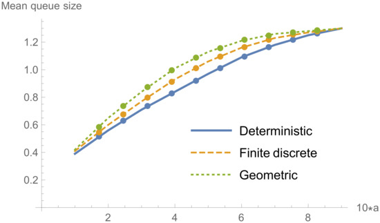
Figure 1.
Mean queue size for deterministic service time distribution.
A similar conclusion can be formulated in the case of finite discrete service time distribution for which appropriate results and presented and visualized in Table 2 and in Figure 2, and for geometric service time distribution (see Table 3 and Figure 3).
Table 2.
Mean queue size for finite discrete service time distribution.
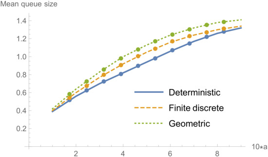
Figure 2.
Mean queue size for finite discrete service time distribution.
Table 3.
Mean queue size for geometric service time distribution.
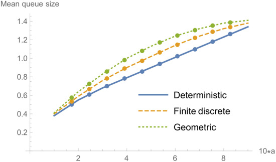
Figure 3.
Mean queue size for geometric service time distribution.
7. Conclusions
In this article, the queue-size distribution is studied in a finite-buffer discrete-time queueing model in which a single vacation policy is implemented. Identifying renewal moments in the evolution of the system and applying the formula of total probability and linear algebra, the representation for the double probability generating function of the transient queue-size distribution is found in a compact form. From the formula, it is possible to obtain the mean stationary queue size just by using the Abelian theorem and differentiation. A numerical study illustrating analytical results is attached. The considered queueing system has potential applications in modeling energy-saving modes or maintenance periods in wireless communication networks, production lines, etc.
Funding
This research received no external funding.
Institutional Review Board Statement
Not applicable.
Informed Consent Statement
Not applicable.
Data Availability Statement
Not applicable.
Conflicts of Interest
The authors declare no conflict of interest.
References
- Meisling, T. Discrete-time queuing theory. Oper. Res. 1958, 6, 96–105. [Google Scholar] [CrossRef]
- Bruneel, H. Performance of discrete-time queueing systems. Comput. Oper. Res. 1993, 20, 303–320. [Google Scholar] [CrossRef]
- Bruneel, H.; Kim, B.G. Discrete-Time Models for Communication Systems Including ATM; Springer Science & Business Media: Berlin/Heidelberg, Germany, 2012. [Google Scholar]
- Takagi, H. Queueing Analysis—A Foundation of Performance Evaluation, Vol. 3. Discrete-Time Systems; North-Holland: Amsterdam, The Netherlands, 1993. [Google Scholar]
- Neuts, M.F. The single server queue in discrete time numerical analysis. Nav. Res. Logist. Q. 1973, 20, 29–304. [Google Scholar] [CrossRef]
- Krishnamoorthy, A.; Pramod, P.K.; Chakravarthy, S.R. Queues with interruptions: A survey. TOP 2014, 22, 290–320. [Google Scholar] [CrossRef]
- Tian, N.; Ma, Z.; Liu, M.. The discrete time Geom/Geom/1 queue with multiple working vacations. Appl. Math. Model. 2008, 32, 2941–2953. [Google Scholar] [CrossRef]
- Tian, N.; Zhang, Z.G. The discrete-time GI/Geo/1 queue with multiple vacations. Queueing Syst. 2002, 40, 283–294. [Google Scholar] [CrossRef]
- Chae, K.C.; Lee, S.-M.; Lee, S.-H. The discrete-time GI/Geo/1 queue with single vacation. Qual. Technol. Quant. Manag. 2008, 5, 21–31. [Google Scholar] [CrossRef]
- Fiems, D.; Bruneel, H. Analysis of a discrete-time queueing system with times vacations. Queueing Syst. 2002, 42, 243–254. [Google Scholar] [CrossRef]
- Alfa, A.S. Vacation models in discrete time. Queueing Syst. 2002, 44, 5–30. [Google Scholar] [CrossRef]
- Li, J.-H.; Tian, N.-S. Analysis of the discrete time Geo/Geo/1 queue with single working vacation. Qual. Technol. Quant. Manag. 2008, 5, 77–89. [Google Scholar] [CrossRef]
- Li, J.-H.; Tian, N.-S. The discrete-time GI/Geo/1 queue with working vacations and vacation interruption. Appl. Math. Comput. 2007, 1, 1–10. [Google Scholar]
- Moreno, P. A discrete-time single-server queueing system under multiple vacations and setup-closedown times. Stoch. Anal. Appl. 2009, 27, 221–239. [Google Scholar] [CrossRef]
- Samanta, S.K. Analysis of a discrete-time GI/Geo/1 queue with single vacation. Int. J. Oper. Res. 2009, 5, 292–310. [Google Scholar] [CrossRef]
- Samanta, S.K.; Gupta, U.C.; Sharma, R.K. Analysis of finite capacity discrete-time GI/Geo/1 queueing system with multiple vacations. J. Oper. Res. Soc. 2007, 58, 368–377. [Google Scholar] [CrossRef]
- Kim, S.J.; Kim, N.K.; Park, H.-M.; Chae, K.C.; Lim, D.-E. On the discrete-time Geo(X)/G/1 queues under N-policy with single and multiple vacations. J. Appl. Math. 2013, 2013, 587163. [Google Scholar] [CrossRef]
- Liu, Z.; Ma, Y.; Zhang, Z.G. Equilibrium mixed strategies in a discrete-time Markovian queue under multiple and single vacation policies. Qual. Technol. Quant. Manag. 2015, 12, 369–382. [Google Scholar] [CrossRef]
- Chydziński, A. On the transient queue with the dropping function. Entropy 2020, 22, 825. [Google Scholar] [CrossRef]
- Tikhonenko, O.; Kempa, W.M. The generalization of AQM algorithms for queueing systems with bounded capacity. Lect. Notes Comput. Sci. 2012, 7204, 242–251. [Google Scholar]
- Bounkhel, M.; Tadj, L.; Hedjar, R. Steady-state analysis of a flexible Markovian queue with server breakdowns. Entropy 2019, 21, 259. [Google Scholar] [CrossRef]
- Kempa, W.M. GI/G/1/∞ batch arrival queueing system with a single exponential vacation. Math. Methods Oper. Res. 2009, 69, 81–97. [Google Scholar] [CrossRef]
- Kempa, W.M. Analysis of departure process in batch arrival queue with multiple vacations and exhaustive service. Commun. Stat. Theory Methods 2011, 40, 2856–2865. [Google Scholar] [CrossRef]
- Kempa, W.M. On transient queue-size distribution in the batch-arrivals system with a single vacation policy. Kybernetika 2014, 50, 126–141. [Google Scholar] [CrossRef][Green Version]
- Kempa, W.M. Transient workload distribution in the M/G/1 finite-buffer queue with single and multiple vacations. Ann. Oper. Res. 2016, 239, 381–400. [Google Scholar] [CrossRef]
- Kempa, W.M. The virtual waiting time for the batch arrival queueing systems. Stoch. Anal. Appl. 2004, 22, 1235–1255. [Google Scholar] [CrossRef]
- Kempa, W.M. A comprehensive study on the queue-size distribution in a finite-buffer system with a general independent input flow. Perform. Eval. 2017, 108, 1–15. [Google Scholar] [CrossRef]
- Baklizi, M. Weight queue dynamic active queue management algorithm. Symmetry 2020, 12, 2077. [Google Scholar] [CrossRef]
- Khan, I.E.; Paramasivam, R. Reduction in waiting time in an M/M/1/N encouraged arrival queue with feedback, balking and maintaining of reneged customers. Symmetry 2022, 14, 1743. [Google Scholar] [CrossRef]
- Yen, T.-C.; Wang, K.-H.; Chen, J.-Y. Optimization analysis of the N-policy M/G/1 queue with working breakdowns. Symmetry 2020, 12, 583. [Google Scholar] [CrossRef]
- Gunavathi, K. Probability and Queueing Theory; S. Chand Publishing: New Delhi, India, 2008. [Google Scholar]
- Nelson, R. Probability, Stochastic Processes, and Queueing Theory: The Mathematics of Computer Performance Modeling; Springer Science & Business Media: Berlin/Heidelberg, Germany, 2013. [Google Scholar]
- Korolyuk, V.S. Boundary-value problems for compound Poisson processes. Theory Probab. Appl. 1974, 19, 1–13. [Google Scholar] [CrossRef]


Publisher’s Note: MDPI stays neutral with regard to jurisdictional claims in published maps and institutional affiliations. |
© 2022 by the author. Licensee MDPI, Basel, Switzerland. This article is an open access article distributed under the terms and conditions of the Creative Commons Attribution (CC BY) license (https://creativecommons.org/licenses/by/4.0/).