Linear Diophantine Fuzzy Rough Sets: A New Rough Set Approach with Decision Making

Abstract

In this article, a new hybrid model named linear Diophantine fuzzy rough set (LDFRS) is proposed to magnify the notion of rough set (RS) and linear Diophantine fuzzy set (LDFS). Concerning the proposed model of LDFRS, it is more efficient to discuss the fuzziness and roughness in terms of linear Diophantine fuzzy approximation spaces (LDFA spaces); it plays a vital role in information analysis, data analysis, and computational intelligence. The concept of $(<\mathfrak{p},{\mathfrak{p}}^{\prime }>,<\mathfrak{q},{\mathfrak{q}}^{\prime }>)$-indiscernibility of a linear Diophantine fuzzy relation (LDF relation) is used for the construction of an LDFRS. Certain properties of LDFA spaces are explored and related results are developed. Moreover, a decision-making technique is developed for modeling uncertainties in decision-making (DM) problems and a practical application of fuzziness and roughness of the proposed model is established for medical diagnosis.

1. Introduction

Due to the growing interest in the development of computational intelligence techniques, classical set theory has been generalized to many beneficial theories and models. Some of the worthwhile set theoretic models are fuzzy sets (FSs) [1], intuitionistic fuzzy sets (IFSs) [2,3], bipolar fuzzy sets (BFSs) [4], rough sets (RSs) [5,6], soft sets (SSs) [7], etc. In 1965, Zadeh [1] introduced the conceptualization of FSs, one of the most successful extensions among the above-mentioned theories. FSs assign grades to all objects of the universal set which lie in the unit interval $[0,1]$ on the basis of their characteristics, instead of only $\{0,1\}$ as in classical set theory. In other words, the elements may have the property of belonging partially to the universal set. For example, we cannot segregate all the patients into two specific classes, i.e., either somebody is ill or not, because an individual’s illness may not be at its earliest or extreme level. In FS theory, an individual who is nauseated could have a degree of illness near to 0.889. In contrast, if somebody has a degree of illness 0.124, this intimates that he has nearly recovered from poor health. Since 1965, FSs have been studied extensively by various authors and innovative mathematical extensions have been developed such as m-polar fuzzy set (mFS) [8], Pythagorean fuzzy set (PFS) [9,10], orthopair fuzzy set (OFS) [11], q-rung orthopair fuzzy set (q-ROFS) [12], and Pythagorean m-polar fuzzy set (PmFS) [13,14].

One of the most recent and an important generalization of FS is LDFS, originated by Riaz and Hashmi [15] in 2019. LDFS is the most convenient mathematical model concerning modeling vagueness in real-life complications. LDFS removes all the restrictions related to the association and non-alignment grades of the prevailing concepts as mentioned above, by the adoption of corresponding control parameters. For DM, multi-attribute decision-making (MADM), engineering, artificial intelligence (AI) and the medical sort, LDFS is the most suitable mathematical structure, where the decision makers have freedom to assign membership grades (MGs) and non-membership grades (NMGs) [15]. Nowadays, LDFSs involve a massive number of vibrant researchers and the study of this paradigm is growing rapidly. Some of the remarkable applications of LDFSs concerning algebraic structures, soft rough sets model, binary relations, and q-linear Diophantine fuzzy are found in [16,17,18].

The binary relation performance is quite influential in distinctive fields of pure and applied sciences. In 1971, Zadeh [19] established the conception of a fuzzy relation (F relation). F relations are very useful for modeling situations, where interactions among various objects are more or less strong. FSs and F relations have voluminous applications in pure and applied sciences. A particular study on FSs and F relations is presented by Wang et al. in [20]. In 1983, Atanassov [21] proposed the idea of intuitionistic fuzzy relation (IF relation) by promulgating the constraint that the sum of association and disassociation grades should not be greater than 1. Recently, Ayub et al. [22], proposed a beautiful extension of the IF relation, named linear Diophantine fuzzy relation (LDF relation), with a robust application in decision-making, by the influence of the novel concepts of LDFSs. Hashmi et al. [23] suggested the conceptualization of m-polar neutrosophic topology with applications to MADM.

Pawlak in 1982 put forward an approach of rough set (RS) in order to cope with the vagueness and incompleteness in information systems. RS theory is also a development of classical set theory, where the objects are analyzed by means of lower and upper approximation spaces. These approximation spaces revealed the obscured awareness in the information system. In RS theory, it is assumed that we have some additional enlightenment about the features of a set. Let us clarify this notion with an example. In the current pandemic situation, we consider a group of some patients of corona virus. In order to investigate corona, one must see its disparate symptoms, for instance, fever, dry cough, tiredness, sore throat, loss of taste or smell, difficulty breathing. Patients exhibiting similar symptoms are equivalent with respect to the available knowledge and form elementary granules of data. RS theory has successful applications to computer sciences, cognitive sciences, artificial intelligence, machine learning, conflict analysis and data analysis.

Since RS theory has been developed, many robust generalizations of RS have been established in various directions. For instance, binary relations [24,25], tolerance relations [26], similarity relations [27], soft binary relations [28,29], soft equivalence relations [30], set valued maps [31], two equivalence relations [32], normal soft group [33], etc. Recently, Shiekh et al. [34] proposed the solution of matrix games with rough interval pay-offs and its application in the telecom market share problem. Shiekh et al. [35] suggested an alternative approach for solving fuzzy matrix games. Ruidas et al. [36] developed a production-repairing inventory model considering demand and the proportion of defective items as rough intervals. They developed two independent models by using the rough interval. The first model concerned demand of the product and the second model concerned both the demand and the defective rate. In the information systems, where attribute values are not numerical, an excessive number of vibrant mathematicians investigated hybridization of FSs and RSs. Cock et al. [37] proposed an innovative model of fuzzy rough sets and developed some forgotten step of roughness. Maji and Garai [38] introduced the notion of IT2 fuzzy rough sets and max-relevance significance criterion with application to attribute selection. Mahmood et al. [39] proposed the lower and upper approximations in quotient groups and homomorphisms between lower and upper approximations. Mahmood et al. [40] studied group homomorphism-based comparison between lower and upper approximations. Tsang et al. [41] developed a new attribute reduction approach based on fuzzy rough sets. Yao et al. [42] introduced a novel variable precision $(\theta ,\sigma )$-fuzzy rough set approach towards fuzzy granules and granular computing. Dubois and H. Prade et al. [43] introduced novel concepts of fuzzy rough sets and rough fuzzy sets. They unveiled a constructive approach, where the approximations are constructed by means of an F relation to be more useful, from an application point of view. Akram et al. [44] suggested a novel hybrid decision-making approach based on intuitionistic fuzzy N-soft rough sets. Shabir and Shaheen [45] explored a new technique to fuzzify a RS when the objects are discernible up to a certain degree $\alpha$. To deal with uncertainty and bipolarity as well in many situations, Malik and Shabir [46] produced fuzzy bipolar soft sets (FBSSs) with utilization in DM. In [47], Gul and Shabir introduced a new idea of roughness of a crisp set based on $(\alpha ,\beta )$-indiscernibilty of a bipolar fuzzy relation (BF relation).

Shabir et al. [48] proposed a new approach to discuss roughness and soft rough sets. Ayub et al. [49] developed some applications of roughness in soft-intersection groups and their approximation spaces. Chen et al. [50] suggested a study of roughness in modules of fractions. Zhang et al. [51] introduced novel classes of fuzzy soft $\beta$-covering-based fuzzy rough sets with applications to MCDM. They developed some results for two different fuzzy soft $\beta$-coverings having the same upper (lower) approximation operators. Ouyang et al. [52] developed tolerance relations for fuzzy rough sets and developed certain interesting results. Sun and Ma [53] suggested a model for fuzzy rough set with applications towards two different universes. Yang and Li [54] introduced the bipolar fuzzy rough set model with applications to two different universes.

Feng et al. [55,56] proposed novel concepts of soft rough set, soft set, and rough sets to analyze certain characteristics of information systems. Zhang et al. [57,58] introduced the notion of the IFS-rough set and interval-valued hesitant fuzzy rough approximation operators. Zhou and Wu [59] developed certain properties of rough set approximations in Atanassov IFS theory. Zhan and Alcantud [60] proposed an algorithm survey of parameter reduction of soft sets. Hussain et al. [61,62] proposed Pythagorean fuzzy soft rough sets, q-Rung orthopair fuzzy soft average aggregation operators and their applications in decision-making. Pamucar [63] proposed a normalized weighted geometric Dombi Bonferroni mean operator with interval grey numbers with application in MCDM. Ali et al. [64] developed Einstein geometric aggregation operators using a novel complex interval-valued Pythagorean fuzzy setting with application in green supplier chain management. Božanic [65] discussed a hybrid LBWA-IR-MAIRCA multi-criteria decision-making model for determination of constructive elements of weapons. Agarwal et al.’s [66] study involved a parametric analysis of a grinding process using the rough sets theory.

Let $ϝ$ be the universe of discourse. Let $\mu ,\nu :ϝ\to [0,1]$ be the membership function (MF) and non-membership function (NMF). Then for any $\hslash \in ϝ$, the terms $\mu (\hslash )$ and $\nu (\hslash )$ represent the membership grade (MG) and non-membership grade (NMG). The following three different representations of a linear Diophantine fuzzy number (LDFN) were used in [15,16,22,67]

$$\begin{array}{ccc}\hfill N& =& \left(\left(\mu \right(\hslash ),\nu (\hslash \left)\right),\left(\alpha \right(\hslash ),\beta (\hslash \left)\right)\right)\hfill \\ & =& \left(<\mu (\hslash ),\nu (\hslash )>,<\alpha (\hslash ),\beta (\hslash )>\right)\hfill \\ & =& ⟨\left(\mu \right(\hslash ),\nu (\hslash \left)\right),\left(\alpha \right(\hslash ),\beta (\hslash \left)\right)⟩\hfill \end{array}$$

where $\mu (\hslash ),\nu (\hslash ),\alpha (\hslash ),\beta (\hslash )\in [0,1]$ and

$$0\le \alpha (\hslash )\mu (\hslash )+\beta (\hslash )\nu (\hslash ))\le 1$$

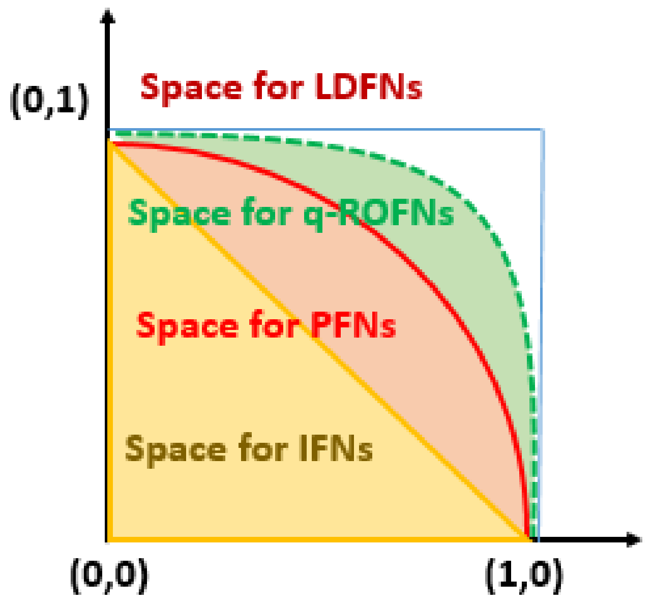
This involves one ordered pair $\left(\mu \right(\hslash ),\nu (\hslash \left)\right)$ containing a pair of MGs and NMGs and a second ordered pair $\left(\alpha \right(\hslash ),\beta (\hslash \left)\right)$ containing reference parameters. A LDFN provides freedom to the decision makers in the selection of MGs and NMGs. Figure 1 and Table 1 demonstrates that the space for LDFNs is broader than the space for IFNs, PFNs and q-ROFNs.

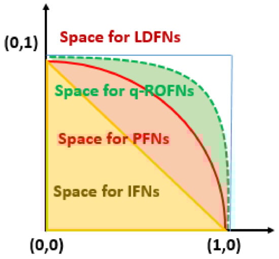
Figure 1. Comparison of LDFNs with IFNs, PFNs and q-ROFNs.

Table 1. Comparison between LDFS with some existing fuzzy sets.

Models	Limitations and Delimitations
Fuzzy sets [1]	A FS assigns MGs but can not deal with NMGs.
IFSs [2,3]	An IFS assigns both MGs and NMGs with $\mu (\hslash )+\nu (\hslash )\le 1$ but it can not deal with $\mu (\hslash )+\nu (\hslash )>1$ $\hslash \in ϝ$.
PFSs [9,10]	A PFS assigns both MGs and NMGs with ${\left(\mu (\hslash )\right)}^2+{\left(\nu (\hslash )\right)}^2\le 1$ but it can not deal with ${\left(\mu (\hslash )\right)}^2+{\left(\nu (\hslash )\right)}^2>1$ $\hslash \in ϝ$.
FFSs [68]	A FFS assigns both MGs and NMGs with ${\left(\mu (\hslash )\right)}^3+{\left(\nu (\hslash )\right)}^3\le 1$ it but can not deal with ${\left(\mu (\hslash )\right)}^3+{\left(\nu (\hslash )\right)}^3>1$ $\hslash \in ϝ$.
q-ROFSs [12]	A q-ROFS assigns both MGs and NMGs with ${\left(\mu (\hslash )\right)}^q+{\left(\nu (\hslash )\right)}^q\le 1,q\ge 1$ but it can not deal with ${\left(\mu (\hslash )\right)}^q+{\left(\nu (\hslash )\right)}^q>1$ or if $\mu (\hslash )=\nu (\hslash )=1$.
LDFSs [15]	A LDFS assign MGs and NMGs as well as the reference/control parameters. It relax the limitations of IFSs, PFSs, FFSs, and q-ROFSs. It provides freedom to decision makers for assigning MGs and NMGs.

Motivated by robust features of RS and LDFS, this work is mainly concerned with the hybridization of these models. Main objectives of this paper are as follows.

• The main objective of this article is to magnify the notion of LDFS and RS for intelligent information processing. The proposed model of LDFRS provides a broader space for the selection of membership and non-membership grades than existing models (FS, IFS, BFS, q-ROFS), to discuss fuzziness and roughness in terms of LDFA spaces. LDFRSs provide freedom to decision makers for assigning membership grades (MGs) and non-membership grades (NMGs).
• The idea of the LDF relation with the addition of control parameters is more efficient for roughness approximation than the existing F relation, IF relation, and BF relation.
• In this paper, we aim to produce an advanced technique for approximation of roughness of a crisp set by using an LDF relation from a universe to another universe based on $(<\mathfrak{p},{\mathfrak{p}}^{\prime }>,<\mathfrak{q},{\mathfrak{q}}^{\prime }>)$-indiscernible objects, that is, the components which do not have completely the same attributes. However, they are similar up to certain degrees $\mathfrak{p},\mathfrak{q},{\mathfrak{p}}^{\prime }$ and ${\mathfrak{q}}^{\prime }$ (say) and involve the fuzziness of the information system if the attribute values are linguistic. Using the above concepts, approximation spaces are then formalized, for approximating the subsets of two universes.
• The abstractions of linear Diophantine fuzzy approximation spaces (LDFA spaces) are defined and related results are explored. Concerning the proposed model of LDFRS, it is more efficient to discuss the fuzziness and roughness in terms of LDFA spaces; it plays a vital role in information analysis and decision analysis.
• Moreover, a decision-making technique is developed for modeling uncertainties in decision-making (DM) problems and a practical application of fuzziness and roughness of proposed model is established for medical diagnosis.

For smooth study of this article, the remainder has the following pattern: In Section 2, a reflection of preliminary abstractions of the RS, LDFS and LDF relation are presented. In Section 3, the concept of Linear diophantine fuzzified rough set (LDFRS) is proposed by employing $(<\mathfrak{p},{\mathfrak{p}}^{\prime }>,<\mathfrak{q},{\mathfrak{q}}^{\prime }>)$-indiscernibility. Some remarkable results related to LDFRS are proved with useful examples. Section 4 presents the intuitions of accuracy measure and roughness measure for $(<\mathfrak{p},{\mathfrak{p}}^{\prime }>,<\mathfrak{q},{\mathfrak{q}}^{\prime }>$ LDFRS. Section 5 presents a utilization of LDFRSs in medical diagnosis with a comparison of Yang et al.’s [54] method. Finally, Section 6 consists of the culmination of this article.

2. Preliminaries

In this subdivision, the ground rules of LDFS, LDF relation and RS are recalled, which are indispensable for the construction of a new hybrid model called Linear Diophantine fuzzy rough set (LDFRS). Throughout this article, $ϝ$, ${ϝ}_1$ and ${ϝ}_2$ will be signified as the universes, unless expressed as something else.

Definition 1

([6]).Let E be an equivalence relation on ϝ. Then, the pair $(ϝ,E)$ is known as an approximation space (A space). For any subset W of ϝ, the lower approximation ${\underline{W}}_E$ and the upper approximation ${\overline{W}}^E$ are described as follows:

$${\underline{W}}_E=\{\hslash \in ϝ:{[\hslash ]}_E\subseteq W\}and{\overline{W}}^E=\{\hslash \in ϝ:{[\hslash ]}_E\cap W\ne \mathsf{\varnothing }\}$$

where ${[\hslash ]}_E$ represents the equivalence class of $\hslash \in ϝ$ determined by E. The boundary region is represented and expressed as below:

$$BR\left(W\right)={\overline{W}}^E-{\underline{W}}_E$$

If $BR\left(W\right)\ne \varnothing$, then W is called a rough set; otherwise it is crisp or definable. Note that:

霳

${\underline{W}}_E$ is known as a positive region of W, which contains the definite members;

霳

$ϝ-{\overline{W}}^E$ is known as a negative region of W, which contains the definite non-members;

霳

$BR\left(W\right)$ contains doubtful members of W, which may or may not contain the members of W.

Definition 2

([15]).An LDFS on ϝ is an object specified as bellow:

$${\mathsf{\Omega }}_{\mathfrak{D}}=\left\{(\hslash ,<\mu (\hslash ),\nu (\hslash )>,<\alpha (\hslash ),\beta (\hslash )>):\hslash \in ϝ\right\}$$

where

$$\mu ,\nu :ϝ\to [0,1]$$

are membership and non-membership functions and $\alpha (\hslash ),\beta (\hslash )\in [0,1]$ are the reference/control parameters of $\mu (\hslash ),\nu (\hslash )$, respectively,with $0\le \alpha (\hslash )\mu (\hslash )+\beta (\hslash )\nu (\hslash )\le 1$ and $0\le \alpha (\hslash )+\beta (\hslash )\le 1$ for all $\hslash \in ϝ$. The dubiety part is prescribed as ${\mathsf{\Psi }}_{\mathfrak{D}}(\hslash ){\mathsf{\Lambda }}_{\mathfrak{D}}(\hslash )=1-(\alpha (\hslash )\mu (\hslash )+\beta (\hslash )\nu (\hslash ))$, where ${\mathsf{\Psi }}_{\mathfrak{D}}(\hslash )$ is known to be the degree of indeterminacy of ℏ to ${\mathsf{\Omega }}_{\mathfrak{D}}$ and ${\mathsf{\Lambda }}_{\mathfrak{D}}(\hslash )$ is the reference parameter related to the degree of indeterminacy. A number of the form $(<\mu (\hslash ),\nu (\hslash )>,<\alpha (\hslash ),\beta (\hslash )>)$ is called linear Diophantine fuzzy number (LDFN).

Recently, Ayub et al. [22] extended the notion of IF relation [21] to LDF relation by making use of reference parameters corresponding to the membership and non-membership grades in the stimulation of Riaz and Hashmi [15].

Definition 3

([22]).An LDF relation R from ${ϝ}_1$ to ${ϝ}_2$ is an expression of the following form:

$$R=\{(({\hslash }_1,{\hslash }_2),<{\mu }_R({\hslash }_1,{\hslash }_2),{\nu }_R({\hslash }_1,{\hslash }_2)>,<\alpha ({\hslash }_1,{\hslash }_2),\beta ({\hslash }_1,{\hslash }_2)>):{\hslash }_1\in {ϝ}_1,{\hslash }_2\in {ϝ}_2\}$$

where the mappings

$${\mu }_R,{\nu }_R:{ϝ}_1\times {ϝ}_2\to [0,1]$$

denote the affiliation and non-membership F relations from ${ϝ}_1$ to ${ϝ}_2$, respectively, and $\alpha ({\hslash }_1,{\hslash }_2),\beta ({\hslash }_1,{\hslash }_2)\in [0,1]$ are the reference parameters corresponding to ${\mu }_R({\hslash }_1,{\hslash }_2)$ and ${\nu }_R({\hslash }_1,{\hslash }_2)$, respectively. These affiliation and non-membership F relations obey the constraint $0\le \alpha ({\hslash }_1,{\hslash }_2){\mu }_R({\hslash }_1,{\hslash }_2)+\beta ({\hslash }_1,{\hslash }_2){\nu }_R({\hslash }_1,{\hslash }_2)\le 1$, for all $({\hslash }_1,{\hslash }_2)\in {ϝ}_1\times {ϝ}_2$ with $0\le \alpha ({\hslash }_1,{\hslash }_2)+\beta ({\hslash }_1,{\hslash }_2)\le 1$. The hesitation part is described as follows:

$$\mho ({\hslash }_1,{\hslash }_2)⊺({\hslash }_1,{\hslash }_2)=1-(\alpha ({\hslash }_1,{\hslash }_2){\mu }_R({\hslash }_1,{\hslash }_2)+\beta ({\hslash }_1,{\hslash }_2){\nu }_R({\hslash }_1,{\hslash }_2))$$

where $⊺({\hslash }_1,{\hslash }_2)$ is an index (a degree) of hesitation whether ${\hslash }_1$ and ${\hslash }_2$ are in the relation R or not and $\mho ({\hslash }_1,{\hslash }_2)$ is the reference parameter of degree of hesitation. For simplicity, we shall use $R=(<{\mu }_R({\hslash }_1,{\hslash }_2),{\nu }_R({\hslash }_1,{\hslash }_2)>,<\alpha ({\hslash }_1,{\hslash }_2),\beta ({\hslash }_1,{\hslash }_2)>)$ for an LDF relation from ${ϝ}_1$ to ${ϝ}_2$. We shall represent the set of all LDF relations from ${ϝ}_1$ to ${ϝ}_2$ by $\mathcal{LDFR}({ϝ}_1\times {ϝ}_2)$.

In the case of finite universes ${ϝ}_1$ and ${ϝ}_2$, the matrix notation of an LDF relation is described below.

Definition 4

([22]).Let $R=(<{\mu }_R({\ell }_i,{\hslash }_j),{\nu }_R({\ell }_i,{\hslash }_j)>,<\alpha ({\ell }_i,{\hslash }_j),\beta ({\ell }_i,{\hslash }_j)>)$ be an LDF relation from ${ϝ}_1$ to ${ϝ}_2$, where ${ϝ}_1=\{{\ell }_1,{\ell }_2,...,{\ell }_m\}$ and ${ϝ}_2=\{{\hslash }_1,{\hslash }_2,...,{\hslash }_n\}$. Consider ${\mu }_R({\ell }_i,{\hslash }_j)={\left({ð}_{ij}\right)}_{m\times n}$, ${\nu }_R({\ell }_i,{\hslash }_j)={\left({ð}_{ij}^{\prime }\right)}_{m\times n}$ and $\alpha ({\ell }_i,{\hslash }_j)={\left({♭}_{ij}\right)}_{m\times n}$, $\beta ({\ell }_i,{\hslash }_j)={\left({♭}_{ij}^{\prime }\right)}_{m\times n}$, with $0\le {♭}_{ij}+{♭}_{ij}^{\prime }\le 1$ and $0\le {♭}_{ij}{ð}_{ij}+{♭}_{ij}^{\prime }{ð}_{ij}^{\prime }\le 1$ for all $i,j$, where $1\le i\le m$ and $1\le j\le n$. Then, an LDF relation R can be symbolized in the following four matrices:

$$\begin{array}{c}{\mu }_R={\left({ð}_{ij}\right)}_{m\times n}=\left(\begin{array}{cccc}{ð}_{11}& {ð}_{12}& ...& {ð}_{1n}\\ {ð}_{21}& {ð}_{22}& ...& {ð}_{2n}\\ .& .& ...& .\\ .& .& ...& .\\ .& .& ...& .\\ {ð}_{m1}& {ð}_{m2}& ...& {ð}_{mn}\end{array}\right), {\nu }_R={\left({ð}_{ij}^{\prime }\right)}_{m\times n}=\left(\begin{array}{cccc}{ð}_{11}^{\prime }& {ð}_{12}^{\prime }& ...& {ð}_{1n}^{\prime }\\ {ð}_{21}^{\prime }& {ð}_{22}^{\prime }& ...& {ð}_{2n}^{\prime }\\ .& .& ...& .\\ .& .& ...& .\\ .& .& ...& .\\ {ð}_{m1}^{\prime }& {ð}_{m2}^{\prime }& ...& {ð}_{mn}^{\prime }\end{array}\right)\end{array}$$

and

$$\begin{array}{c}\alpha ={\left({♭}_{ij}\right)}_{m\times n}=\left(\begin{array}{cccc}{♭}_{11}& {♭}_{12}& ...& {♭}_{1n}\\ {♭}_{21}& {♭}_{22}& ...& {♭}_{2n}\\ .& .& ...& .\\ .& .& ...& .\\ .& .& ...& .\\ {♭}_{m1}& {♭}_{m2}& ...& {♭}_{mn}\end{array}\right), \beta ={\left({♭}_{ij}^{\prime }\right)}_{m\times n}=\left(\begin{array}{cccc}{♭}_{11}^{\prime }& {♭}_{12}^{\prime }& ...& {♭}_{1n}^{\prime }\\ {♭}_{21}^{\prime }& {♭}_{22}^{\prime }& ...& {♭}_{2n}^{\prime }\\ .& .& ...& .\\ .& .& ...& .\\ .& .& ...& .\\ {♭}_{m1}^{\prime }& {♭}_{m2}^{\prime }& ...& {♭}_{mn}^{\prime }\end{array}\right)\end{array}$$

Some fundamental operations on LDF relations are described as follows.

Definition 5

([22]).Let $R_1=(<{\vartheta }_{R_1}^{\mathcal{M}}({\hslash }_1,{\hslash }_2),{\vartheta }_{R_1}^{\mathcal{N}}({\hslash }_1,{\hslash }_2)>,<{\alpha }_1({\hslash }_1,{\hslash }_2),{\beta }_1({\hslash }_1,{\hslash }_2)>)$ and $R_2=(<{\vartheta }_{R_2}^{\mathcal{M}}({\hslash }_1,{\hslash }_2),{\vartheta }_{R_2}^{\mathcal{N}}({\hslash }_1,{\hslash }_2)>,<{\alpha }_2({\hslash }_1,{\hslash }_2),{\beta }_2({\hslash }_1,{\hslash }_2)>)$ be two LDF relations from ${ϝ}_1$ to ${ϝ}_2$. Then,

(1) 

$R_1\subseteq R_2$ if and only if

$${\mu }_{R_1}({\hslash }_1,{\hslash }_2)\le {\mu }_{R_2}({\hslash }_1,{\hslash }_2)and{\vartheta }_{R_1}^{\mathcal{N}}({\hslash }_1,{\hslash }_2)\ge {\vartheta }_{R_2}^{\mathcal{N}}({\hslash }_1,{\hslash }_2),$$

$${\alpha }_1({\hslash }_1,{\hslash }_2)\le {\alpha }_2({\hslash }_1,{\hslash }_2)and{\beta }_1({\hslash }_1,{\hslash }_2)\ge {\beta }_2({\hslash }_1,{\hslash }_2)$$

for all $({\hslash }_1,{\hslash }_2)\in {ϝ}_1\times {ϝ}_2$.

(2) 

$R_1\cup R_2=(<({\mu }_{R_1}\cup {\mu }_{R_2})({\hslash }_1,{\hslash }_2),({\vartheta }_{R_1}^{\mathcal{N}}\cap {\vartheta }_{R_2}^{\mathcal{N}})({\hslash }_1,{\hslash }_2)>,$

$<{\alpha }_1({\hslash }_1,{\hslash }_2)\vee {\alpha }_2({\hslash }_1,{\hslash }_2),{\beta }_1({\hslash }_1,{\hslash }_2)\wedge {\beta }_2({\hslash }_1,{\hslash }_2)>)$, where

$$({\mu }_{R_1}\cup {\mu }_{R_2})({\hslash }_1,{\hslash }_2)={\mu }_{R_1}({\hslash }_1,{\hslash }_2)\vee {\mu }_{R_2}({\hslash }_1,{\hslash }_2)and$$

$$({\vartheta }_{R_1}^{\mathcal{N}}\cap {\vartheta }_{R_2}^{\mathcal{N}})({\hslash }_1,{\hslash }_2)={\vartheta }_{R_1}^{\mathcal{N}}({\hslash }_1,{\hslash }_2)\wedge {\vartheta }_{R_2}^{\mathcal{N}}({\hslash }_1,{\hslash }_2)$$

for all $({\hslash }_1,{\hslash }_2)\in {ϝ}_1\times {ϝ}_2$.

(3) 

$R_1\cap R_2=(<({\mu }_{R_1}\cap {\mu }_{R_2})({\hslash }_1,{\hslash }_2),({\vartheta }_{R_1}^{\mathcal{N}}\cup {\vartheta }_{R_2}^{\mathcal{N}})({\hslash }_1,{\hslash }_2)>,$

$<{\alpha }_1({\hslash }_1,{\hslash }_2)\wedge {\alpha }_2({\hslash }_1,{\hslash }_2),{\beta }_1({\hslash }_1,{\hslash }_2)\vee {\beta }_2({\hslash }_1,{\hslash }_2)>)$, where

$$({\mu }_{R_1}\cap {\mu }_{R_2})({\hslash }_1,{\hslash }_2)={\mu }_{R_1}({\hslash }_1,{\hslash }_2)\wedge {\mu }_{R_2}({\hslash }_1,{\hslash }_2)and$$

$$({\vartheta }_{R_1}^{\mathcal{N}}\cup {\vartheta }_{R_2}^{\mathcal{N}})({\hslash }_1,{\hslash }_2)={\vartheta }_{R_1}^{\mathcal{N}}({\hslash }_1,{\hslash }_2)\vee {\vartheta }_{R_2}^{\mathcal{N}}({\hslash }_1,{\hslash }_2)$$

for all $({\hslash }_1,{\hslash }_2)\in {ϝ}_1\times {ϝ}_2$.

(4) 

$R_1^c=(<{\vartheta }_{R_1}^{\mathcal{N}}({\hslash }_1,{\hslash }_2),{\mu }_{R_1}({\hslash }_1,{\hslash }_2)>,<{\beta }_1({\hslash }_1,{\hslash }_2),{\alpha }_1({\hslash }_1,{\hslash }_2)>)$.

Definition 6

([22]).Let R be an LDF relation on ϝ. Then, R is known as a reflexive LDF relation, if:

$${\mu }_R(\hslash ,\hslash )=1,{\nu }_R(\hslash ,\hslash )=0and\alpha (\hslash ,\hslash )=1,\beta (\hslash ,\hslash )=0$$

for all $\hslash \in ϝ$.

In the case of finite $ϝ$, $R=(<{({ð}_{ij})}_{n\times n},{({ð}_{ij}^{\prime })}_{n\times n}>,<{({♭}_{ij})}_{n\times n},{({♭}_{ij}^{\prime })}_{n\times n}>)$. Then, R is reflexive, if

$${♭}_{ii}={ð}_{ii}=1,\mathrm{and}{♭}_{ii}^{\prime }={ð}_{ii}^{\prime }=0,\mathrm{where}i,j=1,2,...,n.$$

Now, we shall define the $(<\mathfrak{p},{\mathfrak{p}}^{\prime }>,<\mathfrak{q},{\mathfrak{q}}^{\prime }>)$-level cut relation of R according to the encouragement of Riaz et al. [16].

Definition 7.

Let $R=\{(({\hslash }_1,{\hslash }_2),<{\mu }_R({\hslash }_1,{\hslash }_2),{\nu }_R({\hslash }_1,{\hslash }_2)>,<\alpha ({\hslash }_1,{\hslash }_2),\beta ({\hslash }_1,{\hslash }_2)>):{\hslash }_1\in {ϝ}_1,{\hslash }_2\in {ϝ}_2\}$ be an LDF relation from ${ϝ}_1$ to ${ϝ}_2$. For any constants $\mathfrak{p},\mathfrak{q},{\mathfrak{p}}^{\prime },{\mathfrak{q}}^{\prime }\in [0,1]$ such that $0\le \mathfrak{p}\mathfrak{q}+{\mathfrak{p}}^{\prime }{\mathfrak{q}}^{\prime }\le 1$ with $0\le {\mathfrak{p}}^{\prime }+{\mathfrak{q}}^{\prime }\le 1$, define the $(<\mathfrak{p},{\mathfrak{p}}^{\prime }>,<\mathfrak{q},{\mathfrak{q}}^{\prime }>)$-level cut relation of R as follows:

$R_{<\mathfrak{p},{\mathfrak{p}}^{\prime }>}^{<\mathfrak{q},{\mathfrak{q}}^{\prime }>}$

$$=\{({\hslash }_1,{\hslash }_2)\in {ϝ}_1\times {ϝ}_2:{\mu }_R({\hslash }_1,{\hslash }_2)\ge \mathfrak{p},\alpha ({\hslash }_1,{\hslash }_2)\ge {\mathfrak{p}}^{\prime },{\nu }_R({\hslash }_1,{\hslash }_2)\le \mathfrak{q},\beta ({\hslash }_1,{\hslash }_2)\le {\mathfrak{q}}^{\prime }\}$$

where,

$$R_{<\mathfrak{p},{\mathfrak{p}}^{\prime }>}=\{({\hslash }_1,{\hslash }_2)\in {ϝ}_1\times {ϝ}_2:{\mu }_R({\hslash }_1,{\hslash }_2)\ge \mathfrak{p},\alpha ({\hslash }_1,{\hslash }_2)\ge {\mathfrak{p}}^{\prime }\}$$

is said to be the $<\mathfrak{p},{\mathfrak{p}}^{\prime }>$-level cut relation of R, and

$$R^{<\mathfrak{q},{\mathfrak{q}}^{\prime }>}=\{({\hslash }_1,{\hslash }_2)\in {ϝ}_1\times {ϝ}_2:{\nu }_R({\hslash }_1,{\hslash }_2)\le \mathfrak{q},\beta ({\hslash }_1,{\hslash }_2)\le {\mathfrak{q}}^{\prime }\}$$

is called the $<\mathfrak{q},{\mathfrak{q}}^{\prime }>$-level cut relation of R.

Next, we define the indiscernibility criteria of the objects in the case of the LDF relation.

Definition 8.

Let $R=(<{\mu }_R({\hslash }_1,{\hslash }_2),{\nu }_R({\hslash }_1,{\hslash }_2)>,<\alpha ({\hslash }_1,{\hslash }_2),\beta ({\hslash }_1,{\hslash }_2)>)$ be an LDF relation from ${ϝ}_1$ to ${ϝ}_2$ and $\mathfrak{p},{\mathfrak{p}}^{\prime }\in (0,1]$, $\mathfrak{q},{\mathfrak{q}}^{\prime }\in [0,1)$. Then, the objects ${\hslash }_1\in {ϝ}_1$ and ${\hslash }_2\in {ϝ}_2$ are said to be $(<\mathfrak{p},{\mathfrak{p}}^{\prime }>,<\mathfrak{q},{\mathfrak{q}}^{\prime }>)$-indiscernible, if:

$${\mu }_R({\hslash }_1,{\hslash }_2)\ge \mathfrak{p},\alpha ({\hslash }_1,{\hslash }_2)\ge {\mathfrak{p}}^{\prime }and{\nu }_R({\hslash }_1,{\hslash }_2)\le \mathfrak{q},\beta ({\hslash }_1,{\hslash }_2)\le {\mathfrak{q}}^{\prime }.$$

which means that the objects ${\hslash }_1\in {ϝ}_1$ and ${\hslash }_2\in {ϝ}_2$ are related up to a relational degree $\mathfrak{p}$ and its parametric degree ${\mathfrak{p}}^{\prime }$ and non-relational degree $\mathfrak{q}$ and the corresponding parametric degree ${\mathfrak{q}}^{\prime }$, respectively.

If $R\in \mathcal{LDF}({ϝ}_1\times {ϝ}_2)$, then the triplet ✠ $=({ϝ}_1,{ϝ}_2,R)$ is called a linear diophantine fuzzified approximation space (LDFA space).

3. Linear Diophantine Rough Approximations for ($<\mathfrak{p},{\mathfrak{p}}^{\prime }>,<\mathfrak{q},{\mathfrak{q}}^{\prime }>$)-Indiscernible Objects

In [45], Shabir and Shaheen initiated the conception of rough approximations of a set based on the $\alpha$-indiscernibility of a compatible (reflexive and symmetric) F relation. More recent, this notion was extended by Gul and Shabir in [47] by using a compatible BF relation on a universe. In this section, we extend these models to a more general concept of LDFRS with the help of an LDF relation [22] without any extra condition on two variant universes. For this objective, the notions of linear Diophantine fuzzified approximation spaces (LDFA spaces) for any subsets W of ${ϝ}_1$ and $\mathcal{J}$ of ${ϝ}_2$ are defined by employing an LDF relation R from ${ϝ}_1$ to ${ϝ}_2$. Some structural properties related to these LDFA spaces are studied in detail; however, some of the properties are not satisfied in the absence of these extra conditions. We shall discuss all these with illustrative examples.

Definition 9.

Let ✠ $=({ϝ}_1,{ϝ}_2,R)$ be LDFA space. For $\mathfrak{p},{\mathfrak{p}}^{\prime }\in (0,1]\mathrm{and}\mathfrak{q},{\mathfrak{q}}^{\prime }\in [0,1)$, define the $<\mathfrak{p},{\mathfrak{p}}^{\prime }>$-lower, -upper and $<\mathfrak{q},{\mathfrak{q}}^{\prime }>$-lower, -upper LDFA spaces of any subset $\mathcal{J}\subseteq {ϝ}_2$ as follows:

$${\underline{R\left(\mathcal{J}\right)}}_{<\mathfrak{p},{\mathfrak{p}}^{\prime }>}=\{{\hslash }_1\in {ϝ}_1:{\vartheta }_R^{\mathcal{M}}({\hslash }_1,{\hslash }_2)<\mathfrak{p},\alpha ({\hslash }_1,{\hslash }_2)<{\mathfrak{p}}^{\prime },\mathrm{for}\mathrm{all}{\hslash }_2\in {\mathcal{J}}^c\}$$

$${\overline{R\left(\mathcal{J}\right)}}^{<\mathfrak{p},{\mathfrak{p}}^{\prime }>}=\{{\hslash }_1\in {ϝ}_1:{\vartheta }_R^{\mathcal{M}}({\hslash }_1,{\hslash }_2)\ge \mathfrak{p},\alpha ({\hslash }_1,{\hslash }_2)\ge {\mathfrak{p}}^{\prime },\mathrm{for}\mathrm{some}{\hslash }_2\in \mathcal{J}\}$$

$${\underline{R\left(\mathcal{J}\right)}}_{<\mathfrak{q},{\mathfrak{q}}^{\prime }>}=\{{\hslash }_1\in {ϝ}_1:{\vartheta }_R^{\mathcal{N}}({\hslash }_1,{\hslash }_2)\le \mathfrak{q},\beta ({\hslash }_1,{\hslash }_2)\le {\mathfrak{q}}^{\prime },\mathrm{for}\mathrm{some}{\hslash }_2\in \mathcal{J}\}$$

$${\overline{R\left(\mathcal{J}\right)}}^{<\mathfrak{q},{\mathfrak{q}}^{\prime }>}=\{{\hslash }_1\in {ϝ}_1:{\vartheta }_R^{\mathcal{N}}({\hslash }_1,{\hslash }_2)>\mathfrak{q},\beta ({\hslash }_1,{\hslash }_2)>{\mathfrak{q}}^{\prime },\mathrm{for}\mathrm{all}{\hslash }_2\in {\mathcal{J}}^c\}$$

Further, for any subset $W\subseteq {ϝ}_1$, define $<\mathfrak{p},{\mathfrak{p}}^{\prime }>$-lower, -upper and $<\mathfrak{p},{\mathfrak{q}}^{\prime }>$-lower, -upper LDFA spaces as follows:

$${\underline{\left(W\right)R}}_{<\mathfrak{p},{\mathfrak{p}}^{\prime }>}=\{{\hslash }_2\in {ϝ}_2:{\vartheta }_R^{\mathcal{M}}({\hslash }_1,{\hslash }_2)<\mathfrak{p},\alpha ({\hslash }_1,{\hslash }_2)<{\mathfrak{p}}^{\prime },\mathrm{for}\mathrm{all}{\hslash }_1\in W^c\}$$

$${\overline{\left(W\right)R}}^{<\mathfrak{p},{\mathfrak{p}}^{\prime }>}=\{{\hslash }_2\in {ϝ}_2:{\vartheta }_R^{\mathcal{M}}({\hslash }_1,{\hslash }_2)\ge \mathfrak{p},\alpha ({\hslash }_1,{\hslash }_2)\ge {\mathfrak{p}}^{\prime },\mathrm{for}\mathrm{some}{\hslash }_1\in W\}$$

$${\underline{\left(W\right)R}}_{<\mathfrak{q},{\mathfrak{q}}^{\prime }>}=\{{\hslash }_2\in {ϝ}_2:{\vartheta }_R^{\mathcal{N}}({\hslash }_1,{\hslash }_2)\le \mathfrak{q},\beta ({\hslash }_1,{\hslash }_2)\le {\mathfrak{q}}^{\prime },\mathrm{for}\mathrm{some}{\hslash }_1\in W\}$$

$${\overline{\left(W\right)R}}^{<\mathfrak{q},{\mathfrak{q}}^{\prime }>}=\{{\hslash }_2\in {ϝ}_2:{\vartheta }_R^{\mathcal{N}}({\hslash }_1,{\hslash }_2)>\mathfrak{q},\beta ({\hslash }_1,{\hslash }_2)>{\mathfrak{q}}^{\prime },\mathrm{for}\mathrm{all}{\hslash }_1\in W^c\}$$

Note that all the LDFA spaces defined above for $\mathcal{J}\subseteq {ϝ}_2$ are the crisp subsets of ${ϝ}_1$ and for $W\subseteq {ϝ}_1$ the LDFA spaces are the crisp subsets of ${ϝ}_2$. Moreover, in Definition 9, for any subset $W\subseteq {ϝ}_1$,

$$\begin{array}{cc}\hfill {\overline{\left(W\right)R}}^{<\mathfrak{p},{\mathfrak{p}}^{\prime }>}& =\{{\hslash }_2\in {ϝ}_2:{\vartheta }_R^{\mathcal{M}}({\hslash }_1,{\hslash }_2)<\mathfrak{p},\alpha ({\hslash }_1,{\hslash }_2)<{\mathfrak{p}}^{\prime },\mathrm{for}\mathrm{all}{\hslash }_1\in W^c\}\hfill \\ \hfill & =\{{\hslash }_2\in {ϝ}_2:{\left({\vartheta }_R^{\mathcal{M}}\right)}^T({\hslash }_2,{\hslash }_1)<\mathfrak{p},{\left(\alpha \right)}^T({\hslash }_2,{\hslash }_1)<{\mathfrak{p}}^{\prime },\mathrm{for}\mathrm{all}{\hslash }_1\in W^c\}\hfill \end{array}$$

where T denotes the transpose of the matrices ${\mu }_R$ and $\alpha$. Similarly, we can calculate ${\overline{\left(W\right)R}}^{<\mathfrak{q},{\mathfrak{q}}^{\prime }>}$, ${\underline{\left(W\right)R}}_{<\mathfrak{q},{\mathfrak{q}}^{\prime }>}$ and ${\overline{\left(W\right)R}}^{<\mathfrak{q},{\mathfrak{q}}^{\prime }>}$.

In the sequel of this manuscript, ✠ $=({ϝ}_1,{ϝ}_2,R)$ is supposed to be an LDFA space.

Definition 10.

With the same notion as in Definition 9, suppose $\mathcal{J}\subseteq {ϝ}_2$ and $W\subseteq {ϝ}_1$. Then, we define the following four pairs:

$${\underline{LDF}}_{✠}(\mathcal{J})=({\underline{R(\mathcal{J})}}_{<\mathfrak{p},{\mathfrak{p}}^{\prime }>},{\underline{R(\mathcal{J})}}_{<\mathfrak{q},{\mathfrak{q}}^{\prime }>})$$

$${\overline{LDF}}^{✠}(\mathcal{J})=({\overline{R(\mathcal{J})}}^{<\mathfrak{p},{\mathfrak{p}}^{\prime }>},{\overline{R(\mathcal{J})}}^{<\mathfrak{q},{\mathfrak{q}}^{\prime }>})$$

$$(W){\underline{LDF}}_{✠}=({\underline{(W)R}}_{<\mathfrak{p},{\mathfrak{p}}^{\prime }>},{\underline{(W)R}}_{<\mathfrak{q},{\mathfrak{q}}^{\prime }>}),$$

$$(W){\stackrel{̲}{LDF}}^{✠}=({\overline{(W)R}}^{<\mathfrak{p},{\mathfrak{p}}^{\prime }>},{\overline{(W)R}}^{<\mathfrak{q},{\mathfrak{q}}^{\prime }>})$$

are known as $(<\mathfrak{p},{\mathfrak{p}}^{\prime }>,<\mathfrak{q},{\mathfrak{q}}^{\prime }>)$-LDF approximations of $\mathcal{J}$ and W, respectively, with respect to ✠. Moreover, the following sets are then defined:

(1) 

$LDF{P}_{✠}(\mathcal{J})=({\underline{R(\mathcal{J})}}_{<\mathfrak{p},{\mathfrak{p}}^{\prime }>},{\overline{R(\mathcal{J})}}^{<\mathfrak{q},{\mathfrak{q}}^{\prime }>})$,

(2) 

$LDF{N}_{✠}(\mathcal{J})={ϝ}_2-{\overline{LDF}}^{✠}(\mathcal{J})=({({\overline{R(\mathcal{J})}}^{<\mathfrak{p},{\mathfrak{p}}^{\prime }>})}^c,{({\underline{R(\mathcal{J})}}_{<\mathfrak{q},{\mathfrak{q}}^{\prime }>})}^c)$,

(3) 

$LDF{B}_{✠}(\mathcal{J})={\overline{LDF}}^{✠}(\mathcal{J})-{\underline{LDF}}_{✠}(\mathcal{J})=({\overline{R(\mathcal{J})}}^{<\mathfrak{p},{\mathfrak{p}}^{\prime }>}-{\underline{R(\mathcal{J})}}_{<\mathfrak{p},{\mathfrak{p}}^{\prime }>},{\underline{R(\mathcal{J})}}_{<\mathfrak{q},{\mathfrak{q}}^{\prime }>}-{\overline{R(\mathcal{J})}}^{<\mathfrak{q},{\mathfrak{q}}^{\prime }>})$.

These are known as positive, negative and boundary parts of $\mathcal{J}\subseteq {ϝ}_2$. Similar notions can be defined for $W\subseteq {ϝ}_1$.

From Definition 9, we deduce the following result.

Lemma 1.

With the same notations as in Definition 9, assume that $W\subseteq {ϝ}_1$ and $\mathcal{J}\subseteq {ϝ}_2$. Then,

(1) 

${\underline{R\left(\mathcal{J}\right)}}_{<\mathfrak{p},{\mathfrak{p}}^{\prime }>}={\underline{R\left(\mathcal{J}\right)}}_{\mathfrak{p}}\cap {\underline{R\left(\mathcal{J}\right)}}_{{\mathfrak{p}}^{\prime }}$.

(2) 

${\overline{R\left(\mathcal{J}\right)}}^{<\mathfrak{p},{\mathfrak{p}}^{\prime }>}={\overline{R\left(\mathcal{J}\right)}}^{\mathfrak{p}}\cap {\overline{R\left(\mathcal{J}\right)}}^{{\mathfrak{p}}^{\prime }}$.

(3) 

${\underline{R\left(\mathcal{J}\right)}}_{<\mathfrak{q},{\mathfrak{q}}^{\prime }>}={\underline{R\left(\mathcal{J}\right)}}_{\mathfrak{q}}\cap {\underline{R\left(\mathcal{J}\right)}}_{{\mathfrak{q}}^{\prime }}$.

(4) 

${\overline{R\left(\mathcal{J}\right)}}^{<\mathfrak{q},{\mathfrak{q}}^{\prime }>}={\overline{R\left(\mathcal{J}\right)}}^{\mathfrak{q}}\cap {\overline{R\left(\mathcal{J}\right)}}^{{\mathfrak{q}}^{\prime }}$.

(5) 

${\underline{\left(W\right)R}}_{<\mathfrak{p},{\mathfrak{p}}^{\prime }>}={\underline{\left(W\right)R}}_{\mathfrak{p}}\cap {\underline{\left(W\right)R}}_{{\mathfrak{p}}^{\prime }}$.

(6) 

${\overline{\left(W\right)R}}^{<\mathfrak{p},{\mathfrak{p}}^{\prime }>}={\overline{\left(W\right)R}}^{\mathfrak{p}}\cap {\overline{\left(W\right)R}}^{{\mathfrak{p}}^{\prime }}$.

(7) 

${\underline{\left(W\right)R}}_{<\mathfrak{q},{\mathfrak{q}}^{\prime }>}={\underline{\left(W\right)R}}_{\mathfrak{q}}\cap {\underline{\left(W\right)R}}_{{\mathfrak{q}}^{\prime }}$.

(8) 

${\overline{\left(W\right)R}}^{<\mathfrak{q},{\mathfrak{q}}^{\prime }>}={\overline{\left(W\right)R}}^{\mathfrak{q}}\cap {\overline{\left(W\right)R}}^{{\mathfrak{q}}^{\prime }}$.

Proof. 

We shall prove only (1). First, we shall define ${\underline{R\left(\mathcal{J}\right)}}_{\mathfrak{p}}$ and ${\underline{R\left(\mathcal{J}\right)}}_{{\mathfrak{p}}^{\prime }}$.

$${\underline{R\left(\mathcal{J}\right)}}_{\mathfrak{p}}=\{{\hslash }_1\in {ϝ}_1:{\vartheta }_R^{\mathcal{M}}({\hslash }_1,{\hslash }_2)<\mathfrak{p},\mathrm{for}\mathrm{all}{\hslash }_2\in {\mathcal{J}}^c\}$$

$${\underline{R\left(\mathcal{J}\right)}}_{{\mathfrak{p}}^{\prime }}=\{{\hslash }_1\in {ϝ}_1:\alpha ({\hslash }_1,{\hslash }_2)<{\mathfrak{p}}^{\prime },\mathrm{for}\mathrm{all}{\hslash }_2\in {\mathcal{J}}^c\}$$

Now, by Definition 9,

$$\begin{array}{cc}\hfill {\underline{R\left(\mathcal{J}\right)}}_{<\mathfrak{p},{\mathfrak{p}}^{\prime }>}& =\{{\hslash }_1\in {ϝ}_1:{\vartheta }_R^{\mathcal{M}}({\hslash }_1,{\hslash }_2)<\mathfrak{p},\alpha ({\hslash }_1,{\hslash }_2)<{\mathfrak{p}}^{\prime },\mathrm{for}\mathrm{all}{\hslash }_2\in {\mathcal{J}}^c\}\hfill \\ \hfill & =\{{\hslash }_1\in {ϝ}_1:{\vartheta }_R^{\mathcal{M}}({\hslash }_1,{\hslash }_2)<\mathfrak{p},\mathrm{for}\mathrm{all}{\hslash }_2\in {\mathcal{J}}^c\}\hfill \\ \hfill & \cap \{{\hslash }_1\in {ϝ}_1:\alpha ({\hslash }_1,{\hslash }_2)<{\mathfrak{p}}^{\prime },\mathrm{for}\mathrm{all}{\hslash }_2\in {\mathcal{J}}^c\}\hfill \\ \hfill & ={\underline{R\left(\mathcal{J}\right)}}_{\mathfrak{p}}\cap {\underline{R\left(\mathcal{J}\right)}}_{{\mathfrak{p}}^{\prime }}.\hfill \end{array}$$

The remaining parts can be proved in a similar way. □

To explain our new concept given in Definition 9, an example is under consideration.

Example 1.

Let ${ϝ}_1=\{{\mathfrak{c}}_1,{\mathfrak{c}}_2,{\mathfrak{c}}_3,{\mathfrak{c}}_4\}$ and ${ϝ}_2=\{{\mathfrak{c}}_1^{\prime },{\mathfrak{c}}_2^{\prime },{\mathfrak{c}}_3^{\prime }\}$. Construct an LDF relation R from ${ϝ}_1$ to ${ϝ}_2$ in the form of the following matrices:

${\mu }_R=\left(\begin{array}{ccc}0.75& 0.58& 0.65\\ 0.56& 0.42& 0.46\\ 0.68& 0.35& 0.43\\ 0.41& 0.45& 0.44\end{array}\right)$, ${\nu }_R=\left(\begin{array}{ccc}0.70& 0.42& 0.55\\ 0.88& 0.75& 0.45\\ 0.54& 0.32& 0.21\\ 0.46& 0.45& 0.25\end{array}\right)$, and

$\alpha =\left(\begin{array}{ccc}0.50& 0.50& 0.60\\ 0.45& 0.38& 0.30\\ 0.54& 0.39& 0.38\\ 0.50& 0.44& 0.45\end{array}\right)$, $\beta =\left(\begin{array}{ccc}0.50& 0.45& 0.40\\ 0.54& 0.60& 0.56\\ 0.46& 0.58& 0.54\\ 0.49& 0.32& 0.35\end{array}\right)$.

Let $\mathcal{J}=\{{\mathfrak{c}}_1^{\prime },{\mathfrak{c}}_3^{\prime }\}\subseteq {ϝ}_2$. Then, for $\mathfrak{p}=0.58$, ${\mathfrak{p}}^{\prime }=0.50$ and $\mathfrak{q}=0.42$, ${\mathfrak{q}}^{\prime }=0.45$, $(<0.58,0.50>,<0.42,0.45>)$-LDF approximations are given as below:

$${\underline{R\left(\mathcal{J}\right)}}_{<0.58,0.50>}=\{{\mathfrak{c}}_2,{\mathfrak{c}}_3,{\mathfrak{c}}_4\},{\overline{R\left(\mathcal{J}\right)}}^{<0.58,0.50>}=\{{\mathfrak{c}}_1,{\mathfrak{c}}_3\}$$

$${\underline{R\left(\mathcal{J}\right)}}_{<0.42,0.45>}=\left\{{\mathfrak{c}}_4\right\},{\overline{R\left(\mathcal{J}\right)}}^{<0.42,0.45>}=\left\{{\mathfrak{c}}_2\right\}$$

Hence, ${\underline{R\left(\mathcal{J}\right)}}_{<0.58,0.50>}⊈{\overline{R\left(\mathcal{J}\right)}}^{<0.58,0.50>}$ and ${\overline{R\left(\mathcal{J}\right)}}^{<0.42,0.45>}⊈{\underline{R\left(\mathcal{J}\right)}}_{<0.42,0.45>}$. Now, for a subset W of ${ϝ}_1$, we take first the transpose of the above matrices:

${\left({\mu }_R\right)}^T=\left(\begin{array}{cccc}0.75& 0.56& 0.68& 0.41\\ 0.58& 0.42& 0.35& 0.45\\ 0.65& 0.46& 0.43& 0.44\end{array}\right)$, ${\left({\nu }_R\right)}^T=\left(\begin{array}{cccc}0.70& 0.88& 0.54& 0.46\\ 0.42& 0.75& 0.32& 0.45\\ 0.55& 0.45& 0.21& 0.25\end{array}\right)$, and,

${\left(\alpha \right)}^T=\left(\begin{array}{cccc}0.50& 0.45& 0.54& 0.50\\ 0.50& 0.38& 0.39& 0.44\\ 0.60& 0.30& 0.38& 0.45\end{array}\right)$, ${\left(\beta \right)}^T=\left(\begin{array}{cccc}0.50& 0.54& 0.46& 0.50\\ 0.45& 0.60& 0.58& 0.32\\ 0.40& 0.56& 0.54& 0.35\end{array}\right)$.

Suppose that $W=\{{\mathfrak{c}}_2,{\mathfrak{c}}_3,{\mathfrak{c}}_4\}$. Then, for $\mathfrak{p}=0.65$, ${\mathfrak{p}}^{\prime }=0.50$ and $\mathfrak{q}=0.55$, ${\mathfrak{q}}^{\prime }=0.40$, the $(<0.65,0.50>,<0.55,0.40>)$-LDF approximations are:

$${\underline{\left(W\right)R}}_{<0.65,0.50>}=\left\{{\mathfrak{c}}_2^{\prime }\right\},{\overline{\left(W\right)R}}^{<0.65,0.50>}=\left\{{\mathfrak{c}}_1^{\prime }\right\}$$

$${\underline{\left(W\right)R}}_{<0.55,0.40>}=\{{\mathfrak{c}}_2^{\prime },{\mathfrak{c}}_3^{\prime }\},{\overline{\left(W\right)R}}^{<0.55,0.40>}=\left\{{\mathfrak{c}}_1^{\prime }\right\}$$

Thus, ${\underline{\left(W\right)R}}_{<0.65,0.50>}⊈{\overline{\left(W\right)R}}^{<0.65,0.50>}$ and ${\overline{\left(W\right)R}}^{<0.55,0.40>}⊈{\underline{\left(W\right)R}}_{<0.55,0.40>}$.

Further, for $\varnothing \subseteq {ϝ}_2$ and ${ϝ}_2$, assume that $\mathfrak{p}=0.58$, ${\mathfrak{p}}^{\prime }=0.50$, $\mathfrak{q}=0.42$, ${\mathfrak{q}}^{\prime }=0.45$; then, the $(<0.58,0.50>,<0.42,0.45>)$-LDF approximations are as below:

$${\underline{R(\varnothing )}}_{<0.58,0.50>}=\left\{{\mathfrak{c}}_4\right\},{\overline{R(\varnothing )}}^{<0.58,0.50>}=\left\{{\mathfrak{c}}_2\right\},$$

$${\underline{R(\varnothing )}}_{<0.42,0.45>}=\left\{{\mathfrak{c}}_2\right\},{\overline{R(\varnothing )}}^{<0.42,0.45>}=\left\{{\mathfrak{c}}_4\right\},$$

$${\underline{R\left({ϝ}_2\right)}}_{<0.58,0.50>}=\{{\mathfrak{c}}_1,{\mathfrak{c}}_3\},{\overline{R\left({ϝ}_2\right)}}^{<0.58,0.50>}=\{{\mathfrak{c}}_1,{\mathfrak{c}}_3\},$$

$${\underline{R\left({ϝ}_2\right)}}_{<0.42,0.45>}=\{{\mathfrak{c}}_1,{\mathfrak{c}}_4\},{\overline{R\left({ϝ}_2\right)}}^{<0.42,0.45>}=\{{\mathfrak{c}}_3,{\mathfrak{c}}_3\}.$$

Now, for $\varnothing \subseteq {ϝ}_1$ and ${ϝ}_1$, the $(<0.58,0.50>,<0.42,0.45>)$-LDF lower and upper approximations are calculated as follows:

$${\underline{(\varnothing )R}}_{<0.58,0.50>}={ϝ}_2,{\overline{(\varnothing )R}}^{<0.58,0.50>}=\varnothing ,$$

$${\underline{(\varnothing )R}}_{<0.42,0.45>}=\left\{{\mathfrak{c}}_1^{\prime }\right\},{\overline{(\varnothing )R}}^{<0.42,0.45>}=\left\{{\mathfrak{c}}_1^{\prime }\right\},$$

$${\underline{\left({ϝ}_2\right)R}}_{<0.58,0.50>}=\varnothing ,{\overline{\left({ϝ}_2\right)R}}^{<0.58,0.50>}={ϝ}_2,$$

$${\underline{\left({ϝ}_2\right)R}}_{<0.42,0.45>}=\{{\mathfrak{c}}_2^{\prime },{\mathfrak{c}}_3^{\prime }\},{\overline{\left({ϝ}_2\right)R}}^{<0.42,0.45>}=\{{\mathfrak{c}}_2^{\prime },{\mathfrak{c}}_3^{\prime }\}.$$

We note that ${\underline{R(\varnothing )}}_{<\mathfrak{p},{\mathfrak{p}}^{\prime }>}\ne \varnothing \ne {\overline{R(\varnothing )}}^{<\mathfrak{q},{\mathfrak{q}}^{\prime }>}$, ${\underline{R\left({ϝ}_2\right)}}_{<\mathfrak{p},{\mathfrak{p}}^{\prime }>}\ne {ϝ}_1\ne {\overline{R\left({ϝ}_2\right)}}^{<\mathfrak{q},{\mathfrak{q}}^{\prime }>}$, ${\underline{(\varnothing )R}}_{<\mathfrak{p},{\mathfrak{p}}^{\prime }>}\ne \varnothing \ne {\overline{(\varnothing )R}}^{<\mathfrak{q},{\mathfrak{q}}^{\prime }>}$ and ${\underline{\left({ϝ}_1\right)R}}_{<\mathfrak{q},{\mathfrak{q}}^{\prime }>}\ne {ϝ}_2\ne {\overline{\left({ϝ}_1\right)R}}^{<\mathfrak{q},{\mathfrak{q}}^{\prime }>}$ for all $\mathfrak{p},{\mathfrak{p}}^{\prime }\in (0,1]$, $\mathfrak{q},{\mathfrak{q}}^{\prime }\in [0,1)$ (see the following Proposition 1).

Proposition 1.

Let R be a reflexive LDF relation on ${ϝ}_1$ and $\mathfrak{p},{\mathfrak{p}}^{\prime }\in (0,1]$, $\mathfrak{q},{\mathfrak{q}}^{\prime }\in [0,1)$. Then,

(1) 

${\underline{R\left({\mathcal{J}}_1\right)}}_{<\mathfrak{p},{\mathfrak{p}}^{\prime }>}\subseteq {\mathcal{J}}_1\subseteq {\overline{R\left({\mathcal{J}}_1\right)}}^{<\mathfrak{p},{\mathfrak{p}}^{\prime }>}$.

(2) 

${\underline{R\left({\mathcal{J}}_1\right)}}_{<\mathfrak{q},{\mathfrak{q}}^{\prime }>}\supseteq {\mathcal{J}}_1\supseteq {\overline{R\left({\mathcal{J}}_1\right)}}^{<\mathfrak{q},{\mathfrak{q}}^{\prime }>}$.

(3) 

${\underline{R(\varnothing )}}_{<\mathfrak{p},{\mathfrak{p}}^{\prime }>}=\varnothing ={\overline{R(\varnothing )}}^{<\mathfrak{q},{\mathfrak{q}}^{\prime }>}$.

(4) 

${\underline{R(\varnothing )}}_{<\mathfrak{q},{\mathfrak{q}}^{\prime }>}=\varnothing ={\overline{R(\varnothing )}}^{<\mathfrak{q},{\mathfrak{q}}^{\prime }>}$.

(5) 

${\underline{R\left({ϝ}_1\right)}}_{<\mathfrak{p},{\mathfrak{p}}^{\prime }>}={ϝ}_1={\overline{R\left({ϝ}_1\right)}}^{<\mathfrak{q},{\mathfrak{q}}^{\prime }>}$.

(6) 

${\underline{R\left({ϝ}_1\right)}}_{<\mathfrak{q},{\mathfrak{q}}^{\prime }>}={ϝ}_1={\overline{R\left({ϝ}_1\right)}}^{<\mathfrak{q},{\mathfrak{q}}^{\prime }>}$.

Proof. 

We shall prove only (1). Others can be proved in a similar manners. First of all, from Definition 9 it is straightforward that:

$${\underline{R\left({\mathcal{J}}_1\right)}}_{<\mathfrak{p},{\mathfrak{p}}^{\prime }>}\subseteq {\mathcal{J}}_1$$

Now, let $\hslash \in {\mathcal{J}}_1$. Then, ${\mu }_R(\hslash ,\hslash )=1\ge \mathfrak{p}$ and $\alpha (\hslash ,\hslash )=1\ge \mathfrak{p}$ since R is reflexive. This yields that $\hslash \in {\overline{R\left({\mathcal{J}}_1\right)}}^{<\mathfrak{p},{\mathfrak{p}}^{\prime }>}$. Thus, ${\mathcal{J}}_1\subseteq {\overline{R\left({\mathcal{J}}_1\right)}}^{<\mathfrak{p},{\mathfrak{p}}^{\prime }>}$. □

Proposition 2.

Suppose that ${\mathfrak{p}}_1,{\mathfrak{p}}_2,{\mathfrak{p}}_1^{\prime },{\mathfrak{p}}_2^{\prime }\in (0,1]$ and ${\mathfrak{q}}_1,{\mathfrak{q}}_2,{\mathfrak{q}}_1^{\prime },{\mathfrak{q}}_2^{\prime }\in [0,1)$ such that ${\mathfrak{p}}_1\le {\mathfrak{p}}_2$, ${\mathfrak{p}}_1^{\prime }\le {\mathfrak{p}}_2^{\prime }$ and ${\mathfrak{q}}_1\le {\mathfrak{q}}_2$, ${\mathfrak{q}}_1^{\prime }\le {\mathfrak{q}}_2^{\prime }$. For any subset $\mathcal{J}\subseteq {ϝ}_2$, the following assertions hold:

(1) 

${\underline{R\left(\mathcal{J}\right)}}_{<{\mathfrak{p}}_1,{\mathfrak{p}}_1^{\prime }>}\subseteq {\underline{R\left(\mathcal{J}\right)}}_{<{\mathfrak{p}}_2,{\mathfrak{p}}_2^{\prime }>}$,

(2) 

${\overline{R\left(\mathcal{J}\right)}}^{<{\mathfrak{p}}_2,{\mathfrak{p}}_2^{\prime }>}\subseteq {\overline{R\left(\mathcal{J}\right)}}^{<{\mathfrak{p}}_1,{\mathfrak{p}}_1^{\prime }>}$,

(3) 

${\underline{R\left(\mathcal{J}\right)}}_{<{\mathfrak{q}}_1,{\mathfrak{q}}_1^{\prime }>}\subseteq {\underline{R\left(\mathcal{J}\right)}}_{<{\mathfrak{q}}_2,{\mathfrak{q}}_2^{\prime }>}$,

(4) 

${\overline{R\left(\mathcal{J}\right)}}^{<{\mathfrak{q}}_2,{\mathfrak{q}}_2^{\prime }>}\subseteq {\overline{R\left(\mathcal{J}\right)}}^{<{\mathfrak{q}}_1,{\mathfrak{q}}_1^{\prime }>}$,

Proof. 

(1) Let ${\hslash }_1\in {\underline{R\left(\mathcal{J}\right)}}_{<{\mathfrak{p}}_1,{\mathfrak{p}}_1^{\prime }>}$. By Definition 9, ${\mu }_R({\hslash }_1,{\hslash }_2)<{\mathfrak{p}}_1$ and $\alpha ({\hslash }_1,{\hslash }_2)<{{\mathfrak{p}}^{\prime }}_1$, for all ${\hslash }_2\in {\mathcal{J}}^c$. Since ${\mathfrak{p}}_1\le {\mathfrak{p}}_2$ and ${{\mathfrak{p}}^{\prime }}_1\le {{\mathfrak{p}}^{\prime }}_2$, therefore ${\mu }_R({\hslash }_1,{\hslash }_2)<{\mathfrak{p}}_2$ and ${⋋}^{\mathcal{M}}({\hslash }_1,{\hslash }_2)<{\mathfrak{p}}_2$, for all ${\hslash }_2\in {\mathcal{J}}^c$. This proves that ${\hslash }_1\in {\underline{R\left(\mathcal{J}\right)}}_{<{\mathfrak{p}}_2,{\mathfrak{p}}_2^{\prime }>}$.

(2) Let ${\hslash }_1\in {\overline{R\left(\mathcal{J}\right)}}^{<{\mathfrak{p}}_2,{\mathfrak{p}}_2^{\prime }>}$. Then, ${\mu }_R({\hslash }_1,{\hslash }_2)\ge {\mathfrak{p}}_2$ and $\alpha ({\hslash }_1,{\hslash }_2)\ge {\mathfrak{p}}_2^{\prime }$, for some ${\hslash }_2\in \mathcal{J}$ (using Definition 9). However, ${\mathfrak{p}}_1\le {\mathfrak{p}}_2$ and ${\mathfrak{p}}_1^{\prime }\le {\mathfrak{p}}_2^{\prime }$. It follows that ${\mu }_R({\hslash }_1,{\hslash }_2)\ge {{\mathfrak{p}}^{\prime }}_2\ge {{\mathfrak{p}}^{\prime }}_{1}and\alpha ({\hslash }_1,{\hslash }_2)\ge {{\mathfrak{p}}^{\prime }}_2\ge {{\mathfrak{p}}^{\prime }}_1$. Thus, ${\mu }_R({\hslash }_1,{\hslash }_2)\ge {\mathfrak{p}}_{1}and\alpha ({\hslash }_1,{\hslash }_2)\ge {{\mathfrak{p}}^{\prime }}_1$ for some ${\hslash }_2\in \mathcal{J}$. Hence, ${\hslash }_1\in {\overline{R\left(\mathcal{J}\right)}}^{<{\mathfrak{p}}_1,{\mathfrak{p}}_1^{\prime }>}$. (3) and (4) can be proved by using the same methodology as (1) and (2). □

Proposition 3.

With the same assumptions as in Proposition 2, let $W\subseteq {ϝ}_1$. Then,

(1) 

${\underline{\left(W\right)R}}_{<{\mathfrak{p}}_1,{\mathfrak{p}}_1^{\prime }>}\subseteq {\underline{\left(W\right)R}}_{<{\mathfrak{p}}_2,{\mathfrak{p}}_2^{\prime }>}$,

(2) 

${\overline{\left(W\right)R}}^{<{\mathfrak{p}}_2,{\mathfrak{p}}_2^{\prime }>}\subseteq {\overline{\left(W\right)R}}^{<{\mathfrak{p}}_1,{\mathfrak{p}}_1^{\prime }>}$,

(3) 

${\underline{\left(W\right)R}}_{<{\mathfrak{q}}_1,{\mathfrak{q}}_1^{\prime }>}\subseteq {\underline{\left(W\right)R}}_{<{\mathfrak{q}}_2,{\mathfrak{q}}_2^{\prime }>}$,

(4) 

${\overline{\left(W\right)R}}^{<{\mathfrak{q}}_2,{\mathfrak{q}}_2^{\prime }>}\subseteq {\overline{\left(W\right)R}}^{<{\mathfrak{q}}_1,{\mathfrak{q}}_1^{\prime }>}$,

Proof. 

The proof is analogous to the proof of Proposition 2. □

In the following example, it is shown that the inclusions in Proposition 2 may not be replaced with equality.

Example 2.

Let us visit Example 1, where ${ϝ}_1=\{{\mathfrak{c}}_1,{\mathfrak{c}}_2,{\mathfrak{c}}_3,{\mathfrak{c}}_4\}$ and ${ϝ}_2=\{{\mathfrak{c}}_1^{\prime },{\mathfrak{c}}_2^{\prime },{\mathfrak{c}}_3^{\prime }\}$. Considering ${\mathfrak{p}}_1=0.58$, ${\mathfrak{p}}_1^{\prime }=0.50$, ${\mathfrak{q}}_1=0.42$, ${\mathfrak{q}}_1^{\prime }=0.45$, then for $\mathcal{J}=\{{\mathfrak{c}}_1^{\prime },{\mathfrak{c}}_3^{\prime }\}$, the $(<0.58,0.50>,<0.42,0.45>)$-LDF lower and upper approximations are:

$${\underline{R\left(\mathcal{J}\right)}}_{<0.58,0.50>}=\{{\mathfrak{c}}_2,{\mathfrak{c}}_3,{\mathfrak{c}}_4\},{\overline{R\left(\mathcal{J}\right)}}^{<0.58,0.50>}=\{{\mathfrak{c}}_1,{\mathfrak{c}}_3\}$$

$${\underline{R\left(\mathcal{J}\right)}}_{<0.42,0.45>}=\left\{{\mathfrak{c}}_4\right\},{\overline{R\left(\mathcal{J}\right)}}^{<0.42,0.45>}=\left\{{\mathfrak{c}}_2\right\}$$

If ${\mathfrak{p}}_2=0.68$, ${{\mathfrak{p}}^{\prime }}_2=0.54$ and ${\mathfrak{q}}_2=0.54$, ${{\mathfrak{q}}^{\prime }}_2=0.46$, then by using Definition 9, we have:

$${\underline{R\left(\mathcal{J}\right)}}_{<0.68,0.54>}={ϝ}_1,{\overline{R\left(\mathcal{J}\right)}}^{<0.54,0.46>}=\{{\mathfrak{c}}_3,{\mathfrak{c}}_4\}$$

If ${\mathfrak{p}}_2=0.56$, ${{\mathfrak{p}}^{\prime }}_2=0.45$ and ${\mathfrak{q}}_2=0.88$, ${{\mathfrak{q}}^{\prime }}_2=0.54$, then

$${\overline{R\left(\mathcal{J}\right)}}_{<0.56,0.45>}=\{{\mathfrak{c}}_1,{\mathfrak{c}}_2,{\mathfrak{c}}_3\},{\overline{R\left(\mathcal{J}\right)}}^{<0.88,0.54>}=\varnothing$$

It is clear that ${\mathfrak{p}}_1=0.58{<\mathfrak{p}}_2=0.68$ and ${{\mathfrak{p}}^{\prime }}_1=0.50{<{\mathfrak{p}}^{\prime }}_2=0.54$; then ${\underline{R\left(\mathcal{J}\right)}}_{<0.68,0.54>}⊈{\underline{R\left(\mathcal{J}\right)}}_{<0.58,0.50>}$ and ${\mathfrak{p}}_1=0.58>{\mathfrak{p}}_2=0.56$ and ${\mathfrak{p}}_1^{\prime }=0.50>{\mathfrak{p}}_2^{\prime }=0.45$; then ${\overline{R\left(\mathcal{J}\right)}}^{<0.58,0.50>}⊈{\overline{R\left(\mathcal{J}\right)}}^{<0.56,0.45>}$. Moreover, ${\mathfrak{q}}_1=0.42<{\mathfrak{q}}_2=0.54$, ${\mathfrak{q}}_1^{\prime }=0.45<{\mathfrak{q}}_{\mathfrak{2}}^{\prime }=0.46$; then ${\underline{R\left(\mathcal{J}\right)}}_{<0.42,0.45>}⊉{\underline{R\left(\mathcal{J}\right)}}_{<0.54,0.46>}$ and ${\mathfrak{q}}_1=0.42<{\mathfrak{q}}_2=0.88$, ${\mathfrak{q}}_1^{\prime }=0.45<{\mathfrak{q}}_2^{\prime }=0.54$; then ${\overline{R\left(\mathcal{J}\right)}}^{<0.42,0.45>}⊉{\overline{R\left(\mathcal{J}\right)}}^{<0.88,0.54>}$.

Proposition 4.

Let ${\mathcal{J}}_1,{\mathcal{J}}_2\subseteq {ϝ}_2$ be such that ${\mathcal{J}}_1\subseteq {\mathcal{J}}_2$. For $\mathfrak{p},{\mathfrak{p}}^{\prime }\in (0,1]$ and $\mathfrak{q},{\mathfrak{q}}^{\prime }\in [0,1)$, the following assertions hold:

(1) 

${\underline{R\left({\mathcal{J}}_1\right)}}_{<\mathfrak{p},{\mathfrak{p}}^{\prime }>}\subseteq {\underline{R\left({\mathcal{J}}_2\right)}}_{<\mathfrak{p},{\mathfrak{p}}^{\prime }>}$,

(2) 

${\overline{R\left({\mathcal{J}}_1\right)}}^{<\mathfrak{p},{\mathfrak{p}}^{\prime }>}\subseteq {\overline{R\left({\mathcal{J}}_2\right)}}^{<\mathfrak{p},{\mathfrak{p}}^{\prime }>}$,

(3) 

${\underline{R\left({\mathcal{J}}_1\right)}}_{<\mathfrak{q},{\mathfrak{q}}^{\prime }>}\subseteq {\underline{R\left({\mathcal{J}}_2\right)}}_{<\mathfrak{q},{\mathfrak{q}}^{\prime }>}$,

(4) 

${\overline{R\left({\mathcal{J}}_1\right)}}^{<\mathfrak{q},{\mathfrak{q}}^{\prime }>}\subseteq {\overline{R\left({\mathcal{J}}_2\right)}}^{<\mathfrak{q},{\mathfrak{q}}^{\prime }>}$.

Proof. 

We shall prove only (1) and (2); (3) and (4) can be proved in a similar manner.

(1) Let ${\hslash }_1\in {\underline{R\left({\mathcal{J}}_1\right)}}_{<\mathfrak{p},{\mathfrak{p}}^{\prime }>}$. Then, ${\mu }_R({\hslash }_1,{\hslash }_2)<\mathfrak{p}$ and $\alpha ({\hslash }_1,{\hslash }_2)<{\mathfrak{p}}^{\prime }$ for all ${\hslash }_2\in {\mathcal{J}}_1^c$ (see Definition 9). Since ${\mathcal{J}}_1\subseteq {\mathcal{J}}_2$, we have ${\mathcal{J}}_1^c\supseteq {\mathcal{J}}_2^c$. So, particularly, ${\mu }_R({\hslash }_1,{\hslash }_2)<\mathfrak{p}$ and $\alpha ({\hslash }_1,{\hslash }_2)<{\mathfrak{p}}^{\prime }$ for all ${\hslash }_2\in {\mathcal{J}}_2^c$. Thus, ${\hslash }_1\in {\underline{R\left({\mathcal{J}}_2\right)}}_{<\mathfrak{p},{\mathfrak{p}}^{\prime }>}$.

(2) Let ${\hslash }_1\in {\overline{R\left({\mathcal{J}}_1\right)}}^{<\mathfrak{p},{\mathfrak{p}}^{\prime }>}$. By Definition 9, ${\mu }_R({\hslash }_1,{\hslash }_2)\ge \mathfrak{p}$ and $\alpha ({\hslash }_1,{\hslash }_2)\ge {\mathfrak{p}}^{\prime }$ for some ${\hslash }_2\in {\mathcal{J}}_1$. However, ${\mathcal{J}}_1\subseteq {\mathcal{J}}_2$, so ${\mu }_R({\hslash }_1,{\hslash }_2)\ge \mathfrak{p}$ and $\alpha ({\hslash }_1,{\hslash }_2)\ge {\mathfrak{p}}^{\prime }$ for some ${\hslash }_2\in {\mathcal{J}}_2$. Consequently, ${\hslash }_1\in {\overline{R\left(\mathcal{J}\right)}}^{<\mathfrak{p},{\mathfrak{p}}^{\prime }>}$. □

Proposition 5.

Assume the same notations as in Proposition 4; let $W_1,W_2\subseteq {ϝ}_1$ be such that $W_1\subseteq W_2$. Then,

(1) 

${\underline{\left(W_1\right)R}}_{<\mathfrak{p},{\mathfrak{p}}^{\prime }>}\subseteq {\underline{\left(W_2\right)R}}_{<\mathfrak{p},{\mathfrak{p}}^{\prime }>}$,

(2) 

${\overline{\left(W_1\right)R}}^{<\mathfrak{p},{\mathfrak{p}}^{\prime }>}\subseteq {\overline{\left(W_2\right)R}}^{<\mathfrak{p},{\mathfrak{p}}^{\prime }>}$,

(3) 

${\underline{\left(W_1\right)R}}_{<\mathfrak{q},{\mathfrak{q}}^{\prime }>}\subseteq {\underline{\left(W_2\right)R}}_{<\mathfrak{q},{\mathfrak{q}}^{\prime }>}$,

(4) 

${\overline{\left(W_1\right)R}}^{<\mathfrak{q},{\mathfrak{q}}^{\prime }>}\subseteq {\overline{\left(W_2\right)R}}^{<\mathfrak{q},{\mathfrak{q}}^{\prime }>}$.

Proof. 

The proof is analogous to the proof of Proposition 4. □

The sign of equality in Proposition 5 may not hold (see Example 3).

Example 3.

Considering Example 1, assume that ${\mathcal{J}}_1=\left\{c_2^{\prime }\right\}$ and ${\mathcal{J}}_2=\{c_1^{\prime },c_2^{\prime }\}$. So, ${\mathcal{J}}_1\subseteq {\mathcal{J}}_2$. For $\mathfrak{p}=0.58$, ${\mathfrak{p}}^{\prime }=0.50$ and $\mathfrak{q}=0.42$ and ${\mathfrak{q}}^{\prime }=0.45$, we have

$${\underline{R\left({\mathcal{J}}_1\right)}}_{<0.58,0.50>}=\left\{{\mathfrak{c}}_2\right\},{\underline{R\left({\mathcal{J}}_2\right)}}_{<0.58,0.50>}=\{{\mathfrak{c}}_2,{\mathfrak{c}}_3,{\mathfrak{c}}_4\}$$

$${\overline{R\left({\mathcal{J}}_1\right)}}^{<0.58,0.50>}=\left\{{\mathfrak{c}}_2\right\},{\overline{R\left({\mathcal{J}}_2\right)}}^{<0.58,0.50>}=\{{\mathfrak{c}}_1,{\mathfrak{c}}_3\}$$

$${\underline{R\left({\mathcal{J}}_1\right)}}_{<0.42,0.45>}=\left\{{\mathfrak{c}}_1\right\},{\underline{R\left({\mathcal{J}}_2\right)}}_{<0.42,0.45>}=\{{\mathfrak{c}}_1,{\mathfrak{c}}_3\}$$

It is clear that ${\underline{R\left({\mathcal{J}}_2\right)}}_{<0.58,0.50>}⊈{\underline{R\left({\mathcal{J}}_1\right)}}_{<0.58,0.50>}$, ${\overline{R\left({\mathcal{J}}_2\right)}}^{<0.58,0.50>}⊈{\overline{R\left({\mathcal{J}}_1\right)}}^{<0.58,0.50>}$ and ${\underline{R\left({\mathcal{J}}_2\right)}}_{<0.42,0.45>}⊈{\underline{R\left({\mathcal{J}}_1\right)}}_{<0.42,0.45>}$.

Proposition 6.

Let $R_1,R_2\in \mathcal{LDFR}({ϝ}_1\times {ϝ}_2)$ such that $R_1\subseteq R_2$, $\mathfrak{p},{\mathfrak{p}}^{\prime }\in (0,1]$ and $\mathfrak{q},{\mathfrak{q}}^{\prime }\in [0,1)$. Then, for any $\mathcal{J}\subseteq {ϝ}_2$, the following properties hold:

(1) 

${\underline{R_2\left(\mathcal{J}\right)}}_{<\mathfrak{p},{\mathfrak{p}}^{\prime }>}\subseteq {\underline{R_1\left(\mathcal{J}\right)}}_{<\mathfrak{p},{\mathfrak{p}}^{\prime }>}$,

(2) 

${\overline{R_1\left(\mathcal{J}\right)}}^{<\mathfrak{p},{\mathfrak{p}}^{\prime }>}\subseteq {\overline{R_2\left(\mathcal{J}\right)}}^{<\mathfrak{p},{\mathfrak{p}}^{\prime }>}$,

(3) 

${\underline{R_1\left(\mathcal{J}\right)}}_{<\mathfrak{q},{\mathfrak{q}}^{\prime }>}\subseteq {\underline{R_2\left(\mathcal{J}\right)}}_{<\mathfrak{q},{\mathfrak{q}}^{\prime }>}$,

(4) 

${\overline{R_2\left(\mathcal{J}\right)}}^{<\mathfrak{q},{\mathfrak{q}}^{\prime }>}\subseteq {\overline{R_1\left(\mathcal{J}\right)}}^{<\mathfrak{q},{\mathfrak{q}}^{\prime }>}$.

Proof. 

(1) Let ${\hslash }_1\in {\underline{R_2\left(\mathcal{J}\right)}}_{<\mathfrak{p},{\mathfrak{p}}^{\prime }>}$. Then, by Definition 9, ${\mu }_{R_2}({\hslash }_1,{\hslash }_2)<\mathfrak{p}and{\alpha }_2({\hslash }_1,{\hslash }_2)<{\mathfrak{p}}^{\prime }\mathrm{for}\mathrm{all}{\hslash }_2\in {\mathcal{J}}^c$. Since $R_1\subseteq R_2$, we have ${\mu }_{R_1}({\hslash }_1,{\hslash }_2)\le {\vartheta }_{R_2}^M({\hslash }_1,{\hslash }_2)<\mathfrak{p}and{\alpha }_1({\hslash }_1,{\hslash }_2)\le {\alpha }_2({\hslash }_1,{\hslash }_2)<{\mathfrak{p}}^{\prime }\mathrm{for}\mathrm{all}{\hslash }_2\in {\mathcal{J}}^c$. Thus, ${\mu }_{R_1}({\hslash }_1,{\hslash }_2)<\mathfrak{p}and{\alpha }_1({\hslash }_1,{\hslash }_2)<{\mathfrak{p}}^{\prime }\mathrm{for}\mathrm{all}{\hslash }_2\in {\mathcal{J}}^c$. Hence, ${\hslash }_1\in {\underline{R_1\left(\mathcal{J}\right)}}_{<\mathfrak{p},{\mathfrak{p}}^{\prime }>}$.

(2) Suppose ${\hslash }_1\in {\overline{R_1\left(\mathcal{J}\right)}}^{<\mathfrak{p},{\mathfrak{p}}^{\prime }>}$. From Definition 9, ${\mu }_{R_1}({\hslash }_1,{\hslash }_2)\ge \mathfrak{p}and{\alpha }_1({\hslash }_1,{\hslash }_2)\ge {\mathfrak{p}}^{\prime }\mathrm{for}\mathrm{some}{\hslash }_2\in \mathcal{J}$. However, $R_1\subseteq R_2$, so we have

$$\mathfrak{p}\le {\mu }_{R_1}({\hslash }_1,{\hslash }_2)\le {\mu }_{R_2}({\hslash }_1,{\hslash }_2)and{\mathfrak{p}}^{\prime }\le {\alpha }_1({\hslash }_1,{\hslash }_2)\le {\alpha }_2({\hslash }_1,{\hslash }_2)\mathrm{for}\mathrm{some}{\hslash }_2\in \mathcal{J}.$$

Thus, $\mathfrak{p}\le {\mu }_{R_2}({\hslash }_1,{\hslash }_2)and{\mathfrak{p}}^{\prime }\le {\alpha }_1({\hslash }_1,{\hslash }_2)\mathrm{for}\mathrm{some}{\hslash }_2\in \mathcal{J}$. Hence, ${\hslash }_1\in {\overline{R_2\left(\mathcal{J}\right)}}^{<\mathfrak{p},{\mathfrak{p}}^{\prime }>}$. The proof of (3) and (4) is analogous to (1) and (2). □

Proposition 7.

Assuming the same hypothesis as in Proposition 6, for any $W\subseteq {ϝ}_1$, we have:

(1) 

${\underline{\left(W\right)R_2}}_{<\mathfrak{p},{\mathfrak{p}}^{\prime }>}\subseteq {\underline{\left(W\right)R_1}}_{<\mathfrak{p},{\mathfrak{p}}^{\prime }>}$,

(2) 

${\overline{\left(W\right)R_1}}^{<\mathfrak{p},{\mathfrak{p}}^{\prime }>}\subseteq {\overline{\left(W\right)R_2}}^{<\mathfrak{p},{\mathfrak{p}}^{\prime }>}$,

(3) 

${\underline{\left(W\right)R_1}}_{<\mathfrak{q},{\mathfrak{q}}^{\prime }>}\subseteq {\underline{\left(W\right)R_2}}_{<\mathfrak{q},{\mathfrak{q}}^{\prime }>}$,

(4) 

${\overline{\left(W\right)R_2}}^{<\mathfrak{q},{\mathfrak{q}}^{\prime }>}\subseteq {\overline{\left(W\right)R_1}}^{<\mathfrak{q},{\mathfrak{q}}^{\prime }>}$.

Proof. 

It can be proved analogously as Proposition 6. □

Theorem 1.

Let ${\mathcal{J}}_1,{\mathcal{J}}_2\subseteq {ϝ}_2$ and $\mathfrak{p},{\mathfrak{p}}^{\prime }\in (0,1]$. Then, the following assertions hold:

(1) 

${\underline{R\left({\mathcal{J}}_1^c\right)}}_{<\mathfrak{p},{\mathfrak{p}}^{\prime }>}={\left({\overline{R\left({\mathcal{J}}_1\right)}}^{<\mathfrak{p},{\mathfrak{p}}^{\prime }>}\right)}^c$;

(2) 

${\overline{R\left({\mathcal{J}}_1^c\right)}}^{<\mathfrak{p},{\mathfrak{p}}^{\prime }>}={\left({\underline{R\left({\mathcal{J}}_1\right)}}_{<\mathfrak{p},{\mathfrak{p}}^{\prime }>}\right)}^c$.

(3) 

${\underline{R({\mathcal{J}}_1\cap {\mathcal{J}}_2)}}_{<\mathfrak{p},{\mathfrak{p}}^{\prime }>}={\underline{R\left({\mathcal{J}}_1\right)}}_{<\mathfrak{p},{\mathfrak{p}}^{\prime }>}\cap {\underline{R\left({\mathcal{J}}_2\right)}}_{<\mathfrak{p},{\mathfrak{p}}^{\prime }>}$;

(4) 

${\underline{R({\mathcal{J}}_1\cup {\mathcal{J}}_2)}}_{<\mathfrak{p},{\mathfrak{p}}^{\prime }>}\supseteq {\underline{R\left({\mathcal{J}}_1\right)}}_{<\mathfrak{p},{\mathfrak{p}}^{\prime }>}\cup {\underline{R\left({\mathcal{J}}_2\right)}}_{<\mathfrak{p},{\mathfrak{p}}^{\prime }>}$;

(5) 

${\overline{R({\mathcal{J}}_1\cup {\mathcal{J}}_2)}}^{<\mathfrak{p},{\mathfrak{p}}^{\prime }>}={\overline{R\left({\mathcal{J}}_1\right)}}^{<\mathfrak{p},{\mathfrak{p}}^{\prime }>}\cup {\overline{R\left({\mathcal{J}}_2\right)}}^{<\mathfrak{p},{\mathfrak{p}}^{\prime }>}$;

(6) 

${\overline{R({\mathcal{J}}_1\cap {\mathcal{J}}_2)}}^{<\mathfrak{p},{\mathfrak{p}}^{\prime }>}\subseteq {\overline{R\left({\mathcal{J}}_1\right)}}^{<\mathfrak{p},{\mathfrak{p}}^{\prime }>}\cap {\overline{R\left({\mathcal{J}}_2\right)}}^{<\mathfrak{p},{\mathfrak{p}}^{\prime }>}$.

Proof. 

(1) Let ${\hslash }_1\in {\underline{R\left({\mathcal{J}}_1^c\right)}}_{<\mathfrak{p},{\mathfrak{p}}^{\prime }>}$. Then, ${\mu }_R({\hslash }_1,{\hslash }_2)<\mathfrak{p}and\alpha ({\hslash }_1,{\hslash }_2)<{\mathfrak{p}}^{\prime }\mathrm{for}\mathrm{all}{\hslash }_2\in {\left({\mathcal{J}}_1^c\right)}^c={\mathcal{J}}_1$. Thus, ${\mu }_R({\hslash }_1,{\hslash }_2)\ngeqq \mathfrak{p}$ and $\alpha ({\hslash }_1,{\hslash }_2)\ngeqq {\mathfrak{p}}^{\prime }$ for all ${\hslash }_2\in {\mathcal{J}}_1$. This implies that ${\hslash }_1\notin {\overline{R\left({\mathcal{J}}_1\right)}}^{<\mathfrak{p},{\mathfrak{p}}^{\prime }>}$. Therefore, ${\hslash }_1\in {\left({\overline{R\left({\mathcal{J}}_1\right)}}^{<\mathfrak{p},{\mathfrak{p}}^{\prime }>}\right)}^c$. Hence, ${\underline{R\left({\mathcal{J}}_1^c\right)}}_{<\mathfrak{p},{\mathfrak{p}}^{\prime }>}\subseteq {\left({\overline{R\left({\mathcal{J}}_1\right)}}^{<\mathfrak{p},{\mathfrak{p}}^{\prime }>}\right)}^c$. The reverse inclusion can be proved by following similar lines.

(2) This proof is analogous to the proof of (1).

Now, to prove (3)–(6), we know that ${\mathcal{J}}_1\cap {\mathcal{J}}_2\subseteq {\mathcal{J}}_1$ and ${\mathcal{J}}_1\cap {\mathcal{J}}_2\subseteq {\mathcal{J}}_2$; then

$${\underline{R({\mathcal{J}}_1\cap {\mathcal{J}}_2)}}_{<\mathfrak{p},{\mathfrak{p}}^{\prime }>}\subseteq {\underline{R\left({\mathcal{J}}_1\right)}}_{<\mathfrak{p},{\mathfrak{p}}^{\prime }>}\cap {\underline{R\left({\mathcal{J}}_2\right)}}_{<\mathfrak{p},{\mathfrak{p}}^{\prime }>}.$$

(1)

$${\overline{R({\mathcal{J}}_1\cap {\mathcal{J}}_2)}}^{<\mathfrak{p},{\mathfrak{p}}^{\prime }>}\subseteq {\overline{R\left({\mathcal{J}}_1\right)}}^{<\mathfrak{p},{\mathfrak{p}}^{\prime }>}\cap {\overline{R\left({\mathcal{J}}_2\right)}}^{<\mathfrak{p},{\mathfrak{p}}^{\prime }>}$$

(2)

(see Proposition 4 (1) and (2), respectively). Further, ${\mathcal{J}}_1\subseteq {\mathcal{J}}_1\cup {\mathcal{J}}_2$ and ${\mathcal{J}}_2\subseteq {\mathcal{J}}_1\cup {\mathcal{J}}_2$; then by using Proposition 4 (3) and (4), respectively, we get:

$${\underline{R({\mathcal{J}}_1\cup {\mathcal{J}}_2)}}_{<\mathfrak{p},{\mathfrak{p}}^{\prime }>}\supseteq {\underline{R\left({\mathcal{J}}_1\right)}}_{<\mathfrak{p},{\mathfrak{p}}^{\prime }>}\cup {\underline{R\left({\mathcal{J}}_2\right)}}_{<\mathfrak{p},{\mathfrak{p}}^{\prime }>}$$

(3)

$${\overline{R({\mathcal{J}}_1\cup {\mathcal{J}}_2)}}^{<\mathfrak{p},{\mathfrak{p}}^{\prime }>}\supseteq {\overline{R\left({\mathcal{J}}_1\right)}}^{<\mathfrak{p},{\mathfrak{p}}^{\prime }>}\cup {\overline{R\left({\mathcal{J}}_2\right)}}^{<\mathfrak{p},{\mathfrak{p}}^{\prime }>}$$

(4)

To prove the converse of the inclusion 1, assume that ${\hslash }_1\in {\underline{R\left({\mathcal{J}}_1\right)}}_{<\mathfrak{p},{\mathfrak{p}}^{\prime }>}\cap {\underline{R\left({\mathcal{J}}_2\right)}}_{<\mathfrak{p},{\mathfrak{p}}^{\prime }>}$. Then, ${\hslash }_1\in {\underline{R\left({\mathcal{J}}_1\right)}}_{<\mathfrak{p},{\mathfrak{p}}^{\prime }>}$ and ${\hslash }_1\in {\underline{R\left({\mathcal{J}}_2\right)}}_{<\mathfrak{p},{\mathfrak{p}}^{\prime }>}$. Using Definition 9, ${\mu }_R({\hslash }_1,{\hslash }_2)<\mathfrak{p},\alpha ({\hslash }_1,{\hslash }_2)<{\mathfrak{p}}^{\prime }$ for all ${\hslash }_2\in {\mathcal{J}}_1^c$ and ${\mu }_R({\hslash }_1,{\hslash }_3)<\mathfrak{p},\alpha ({\hslash }_1,{\hslash }_3)<{\mathfrak{p}}^{\prime }$ for all ${\hslash }_3\in {\mathcal{J}}_2^c$, respectively. Since ${\hslash }_2\in {\mathcal{J}}_1^c$ and ${\hslash }_3\in {\mathcal{J}}_2^c$; then ${\hslash }_2,{\hslash }_3\in {\mathcal{J}}_1^c\cup {\mathcal{J}}_2^c={({\mathcal{J}}_1\cap {\mathcal{J}}_2)}^c$. This yields that ${\mu }_R({\hslash }_1,{\hslash }^{\prime })<\mathfrak{p}$ and $\alpha ({\hslash }_1,{\hslash }^{\prime })<{\mathfrak{p}}^{\prime }$ for all ${\hslash }^{\prime }\in {({\mathcal{J}}_1\cap {\mathcal{J}}_2)}^c$. Thus, ${\hslash }_1\in {\underline{R({\mathcal{J}}_1\cap {\mathcal{J}}_2)}}_{<\mathfrak{p},{\mathfrak{p}}^{\prime }>}$. Hence,

$${\underline{R\left({\mathcal{J}}_1\right)}}_{<\mathfrak{p},{\mathfrak{p}}^{\prime }>}\cap {\underline{R\left({\mathcal{J}}_2\right)}}_{<\mathfrak{p},{\mathfrak{p}}^{\prime }>}\subseteq {\underline{R({\mathcal{J}}_1\cap {\mathcal{J}}_2)}}_{<\mathfrak{p},{\mathfrak{p}}^{\prime }>}$$

Now, to prove the reverse containment of (4), consider ${\hslash }_1\in {\overline{R({\mathcal{J}}_1\cup {\mathcal{J}}_2)}}^{<\mathfrak{p},{\mathfrak{p}}^{\prime }>}$. By Definition 9, there exists ${\hslash }_2\in {\mathcal{J}}_1\cup {\mathcal{J}}_2$ such that ${\mu }_R({\hslash }_1,{\hslash }_2)\ge \mathfrak{p},\alpha ({\hslash }_1,{\hslash }_2)\ge {\mathfrak{p}}^{\prime }$. Thus ${\mu }_R({\hslash }_1,{\hslash }_2)\ge \mathfrak{p},\alpha ({\hslash }_1,{\hslash }_2)\ge {\mathfrak{p}}^{\prime }$ for some ${\hslash }_2\in W$ or ${\mu }_R({\hslash }_1,{\hslash }_2)\ge \mathfrak{p},\alpha ({\hslash }_1,{\hslash }_2)\ge {\mathfrak{p}}^{\prime }$ for some ${\hslash }_2\in W_2$. This proves that ${\hslash }_1\in {\overline{R\left({\mathcal{J}}_1\right)}}^{<\mathfrak{p},{\mathfrak{p}}^{\prime }>}\cup {\overline{R\left({\mathcal{J}}_2\right)}}^{<\mathfrak{p},{\mathfrak{p}}^{\prime }>}$. Hence,

$${\overline{R({\mathcal{J}}_1\cup {\mathcal{J}}_2)}}^{<\mathfrak{p},{\mathfrak{p}}^{\prime }>}\subseteq {\overline{R\left({\mathcal{J}}_1\right)}}^{<\mathfrak{p},{\mathfrak{p}}^{\prime }>}\cup {\overline{R\left({\mathcal{J}}_2\right)}}^{<\mathfrak{p},{\mathfrak{p}}^{\prime }>}.$$

This completes the proof. □

Theorem 2.

Suppose that $W_1,W_2\subseteq {ϝ}_2$ and $\mathfrak{p},{\mathfrak{p}}^{\prime }\in (0,1]$. Then,

(1) 

${\underline{\left(W_1^c\right)R}}_{<\mathfrak{p},{\mathfrak{p}}^{\prime }>}={\left({\overline{\left(W_1\right)R}}^{<\mathfrak{p},{\mathfrak{p}}^{\prime }>}\right)}^c$;

(2) 

${\overline{\left(W_1^c\right)R}}^{<\mathfrak{p},{\mathfrak{p}}^{\prime }>}={\left({\underline{\left(W_1\right)R}}_{<\mathfrak{p},{\mathfrak{p}}^{\prime }>}\right)}^c$.

(3) 

${\underline{(W_1\cap W_2)R}}_{<\mathfrak{p},{\mathfrak{p}}^{\prime }>}={\underline{\left(W_1\right)R}}_{<\mathfrak{p},{\mathfrak{p}}^{\prime }>}\cap {\underline{\left(W_2\right)R}}_{<\mathfrak{p},{\mathfrak{p}}^{\prime }>}$;

(4) 

${\underline{(W_1\cup W_2)R}}_{<\mathfrak{p},{\mathfrak{p}}^{\prime }>}\supseteq {\underline{\left(W_1\right)R}}_{<\mathfrak{p},{\mathfrak{p}}^{\prime }>}\cup {\underline{\left(W_2\right)R}}_{<\mathfrak{p},{\mathfrak{p}}^{\prime }>}$;

(5) 

${\overline{(W_1\cup W_2)R}}^{<\mathfrak{p},{\mathfrak{p}}^{\prime }>}={\overline{\left(W_1\right)R}}^{<\mathfrak{p},{\mathfrak{p}}^{\prime }>}\cup {\overline{\left(W_2\right)R}}^{<\mathfrak{p},{\mathfrak{p}}^{\prime }>}$;

(6) 

${\overline{(W_1\cap W_2)R}}^{<\mathfrak{p},{\mathfrak{p}}^{\prime }>}\subseteq {\overline{\left(W_1\right)R}}^{<\mathfrak{p},{\mathfrak{p}}^{\prime }>}\cap {\overline{\left(W_2\right)R}}^{<\mathfrak{p},{\mathfrak{p}}^{\prime }>}$.

Proof. 

This can be proved by following the same methodology as Theorem 1. □

Theorem 3.

With the same notations as in Theorem 1, let $\mathfrak{q},{\mathfrak{q}}^{\prime }\in [0,1)$. Then,

(1) 

${\underline{R\left({\mathcal{J}}_1^c\right)}}_{<\mathfrak{q},{\mathfrak{q}}^{\prime }>}={\left({\overline{R\left({\mathcal{J}}_1\right)}}^{<\mathfrak{q},{\mathfrak{q}}^{\prime }>}\right)}^c$;

(2) 

${\overline{R\left({\mathcal{J}}_1^c\right)}}^{<\mathfrak{q},{\mathfrak{q}}^{\prime }>}={\left({\underline{R\left({\mathcal{J}}_1\right)}}_{<\mathfrak{q},{\mathfrak{q}}^{\prime }>}\right)}^c$;

(3) 

${\underline{R({\mathcal{J}}_1\cap {\mathcal{J}}_2)}}_{<\mathfrak{q},{\mathfrak{q}}^{\prime }>}\subseteq {\underline{R\left({\mathcal{J}}_1\right)}}_{<\mathfrak{q},{\mathfrak{q}}^{\prime }>}\cap {\underline{R\left({\mathcal{J}}_2\right)}}_{<\mathfrak{q},{\mathfrak{q}}^{\prime }>}$;

(4) 

${\underline{R({\mathcal{J}}_1\cup {\mathcal{J}}_2)}}_{<\mathfrak{q},{\mathfrak{q}}^{\prime }>}={\underline{R\left({\mathcal{J}}_1\right)}}_{<\mathfrak{q},{\mathfrak{q}}^{\prime }>}\cup {\underline{R\left({\mathcal{J}}_2\right)}}_{<\mathfrak{q},{\mathfrak{q}}^{\prime }>}$;

(5) 

${\overline{R({\mathcal{J}}_1\cup {\mathcal{J}}_2)}}^{<\mathfrak{q},{\mathfrak{q}}^{\prime }>}\supseteq {\overline{R\left({\mathcal{J}}_1\right)}}^{<\mathfrak{q},{\mathfrak{q}}^{\prime }>}\cup {\overline{R\left({\mathcal{J}}_2\right)}}^{<\mathfrak{q},{\mathfrak{q}}^{\prime }>}$;

(6) 

${\overline{R({\mathcal{J}}_1\cap {\mathcal{J}}_2)}}^{<\mathfrak{q},{\mathfrak{q}}^{\prime }>}={\overline{R\left({\mathcal{J}}_1\right)}}^{<\mathfrak{q},{\mathfrak{q}}^{\prime }>}\cap {\overline{R\left({\mathcal{J}}_2\right)}}^{<\mathfrak{q},{\mathfrak{q}}^{\prime }>}$.

Proof. 

This can be proved by using similar arguments as in Theorem 1. □

Theorem 4.

Assume the same notations as in Theorem 2, let $\mathfrak{q},{\mathfrak{q}}^{\prime }\in [0,1)$. Then,

(1) 

${\underline{\left(W_1^c\right)R}}_{<\mathfrak{q},{\mathfrak{q}}^{\prime }>}={\left({\overline{\left(W_1\right)R}}^{<\mathfrak{q},{\mathfrak{q}}^{\prime }>}\right)}^c$;

(2) 

${\overline{\left(W_1^c\right)R}}^{<\mathfrak{q},{\mathfrak{q}}^{\prime }>}={\left({\underline{\left(W_1\right)R}}_{<\mathfrak{q},{\mathfrak{q}}^{\prime }>}\right)}^c$;

(3) 

${\underline{(W_1\cap W_2)R}}_{<\mathfrak{q},{\mathfrak{q}}^{\prime }>}\subseteq {\underline{\left(W_1\right)R}}_{<\mathfrak{q},{\mathfrak{q}}^{\prime }>}\cap {\underline{\left(W_2\right)R}}_{<\mathfrak{q},{\mathfrak{q}}^{\prime }>}$;

(4) 

${\underline{(W_1\cup W_2)R}}_{<\mathfrak{q},{\mathfrak{q}}^{\prime }>}={\underline{\left(W_1\right)R}}_{<\mathfrak{q},{\mathfrak{q}}^{\prime }>}\cup {\underline{\left(W_2\right)R}}_{<\mathfrak{q},{\mathfrak{q}}^{\prime }>}$;

(5) 

${\overline{(W_1\cup W_2)R}}^{<\mathfrak{q},{\mathfrak{q}}^{\prime }>}\supseteq {\overline{\left(W_1\right)R}}^{<\mathfrak{q},{\mathfrak{q}}^{\prime }>}\cup {\overline{\left(W_2\right)R}}^{<\mathfrak{q},{\mathfrak{q}}^{\prime }>}$;

(6) 

${\overline{(W_1\cap W_2)R}}^{<\mathfrak{q},{\mathfrak{q}}^{\prime }>}={\overline{\left(W_1\right)R}}^{<\mathfrak{q},{\mathfrak{q}}^{\prime }>}\cap {\overline{\left(W_2\right)R}}^{<\mathfrak{q},{\mathfrak{q}}^{\prime }>}$.

Proof. 

This proof is similar to the proof of Theorem 3. □

4. Accuracy and Roughness Measure for $(<\mathfrak{p},{\mathfrak{p}}^{\prime }>,<\mathfrak{q},{\mathfrak{q}}^{\prime }>)$-Linear Diophantine Rough Sets

In 1982, Pawlak gave the idea of accuracy measure (AM) and roughness measure (RM) to characterize the impreciseness of RS. These numerical measures give us a perception concerning the accuracy of the data related with some equivalence relation for a particular classification. In this Section, we formalize the notion of AM and RM for $(<\mathfrak{p},{\mathfrak{p}}^{\prime }>,<\mathfrak{q},{\mathfrak{q}}^{\prime }>)$-LDFRSs.

Given a Pawlak approximation space $P=(ϝ,E)$, where E is an equivalence relation on $ϝ$, the AM and RM of a subset W of $ϝ$ are described as below:

$${\gamma }_E\left(W\right)=\frac{\underline{E\left(W\right)}}{\overline{E}\left(W\right)}\mathrm{and}{\pi }_E\left(W\right)=1-{\gamma }_E\left(W\right).$$

By following the same pattern, we define the following notions.

Definition 11.

Let ✠ $=({ϝ}_1,{ϝ}_2,R)$ be an LDFA space. For non-empty subsets $\mathcal{J}$ of ${ϝ}_2$ and W of ${ϝ}_1$, define the MA for $(<\mathfrak{p},{\mathfrak{p}}^{\prime }>,<\mathfrak{q},{\mathfrak{q}}^{\prime }>)$-LDFRS with respect to $\mathcal{J}$ and W by the following two pairs, respectively:

$$\mathfrak{AM}\left(\mathcal{J}\right)=({\tau }_{\mathcal{J}}^{<\mathfrak{p},{\mathfrak{p}}^{\prime }>},{\tau }_{\mathcal{J}}^{<\mathfrak{q},{\mathfrak{q}}^{\prime }>})and\mathfrak{AM}\left(W\right)=({\tau }_W^{<\mathfrak{p},{\mathfrak{p}}^{\prime }>},{\tau }_W^{<\mathfrak{q},{\mathfrak{q}}^{\prime }>})$$

where

$${\tau }_{\mathcal{J}}^{<\mathfrak{p},{\mathfrak{p}}^{\prime }>}=\frac{|{\underline{R\left(\mathcal{J}\right)}}_{<\mathfrak{p},{\mathfrak{p}}^{\prime }>}|}{|{\overline{R\left(\mathcal{J}\right)}}^{<\mathfrak{p},{\mathfrak{p}}^{\prime }>}|}and{\tau }_{\mathcal{J}}^{<\mathfrak{q},{\mathfrak{q}}^{\prime }>}=\frac{|{\overline{R\left(\mathcal{J}\right)}}^{<\mathfrak{q},{\mathfrak{q}}^{\prime }>}|}{|{\underline{R\left(\mathcal{J}\right)}}_{<\mathfrak{q},{\mathfrak{q}}^{\prime }>}|}.$$

$${\tau }_W^{<\mathfrak{p},{\mathfrak{p}}^{\prime }>}=\frac{|{\underline{\left(W\right)R}}_{<\mathfrak{p},{\mathfrak{q}}^{\prime }>}|}{|{\overline{\left(W\right)R}}^{<\mathfrak{q},{\mathfrak{q}}^{\prime }>}|}and{\tau }_W^{<\mathfrak{q},{\mathfrak{q}}^{\prime }>}=\frac{|{\overline{\left(W\right)R}}^{<\mathfrak{q},{\mathfrak{q}}^{\prime }>}|}{|{\underline{\left(W\right)R}}_{<\mathfrak{q},{\mathfrak{q}}^{\prime }>}|}.$$

Here, $|.|$ denotes the number of elements in the sets. Next, we define the MR for $(<\mathfrak{p},{\mathfrak{p}}^{\prime }>,<\mathfrak{q},{\mathfrak{q}}^{\prime }>)$-LDFRS with respect to $\mathcal{J}$ and W, respectively, as follows:

$$\mathfrak{RM}\left(\mathcal{J}\right)=(1,1)-\mathfrak{AM}\left(\mathcal{J}\right)=(1,1)-({\tau }_{\mathcal{J}}^{<\mathfrak{p},{\mathfrak{p}}^{\prime }>},{\tau }_{\mathcal{J}}^{<\mathfrak{q},{\mathfrak{q}}^{\prime }>})$$

$$\mathfrak{RM}\left(W\right)=(1,1)-\mathfrak{AM}\left(W\right)=(1,1)-({\tau }_W^{<\mathfrak{p},{\mathfrak{p}}^{\prime }>},{\tau }_W^{<\mathfrak{q},{\mathfrak{q}}^{\prime }>})$$

Remark 1.

From the above Definition 11, we infer the following points:

(1) 

${\tau }_{\mathcal{J}}^{<\mathfrak{p},{\mathfrak{p}}^{\prime }>},{\tau }_{\mathcal{J}}^{<\mathfrak{q},{\mathfrak{q}}^{\prime }>},{\tau }_W^{<\mathfrak{p},{\mathfrak{p}}^{\prime }>},{\tau }_W^{<\mathfrak{q},{\mathfrak{q}}^{\prime }>}\in \mathbb{R}$ since R is not reflexive (see Example 1).

(2) 

If $R\in \mathcal{LDFR}({ϝ}_1\times {ϝ}_1)$ is reflexive, then:

(i) 

${\tau }_{\mathcal{J}}^{<\mathfrak{p},{\mathfrak{p}}^{\prime }>},{\tau }_{\mathcal{J}}^{<\mathfrak{q},{\mathfrak{q}}^{\prime }>},{\tau }_W^{<\mathfrak{p},{\mathfrak{p}}^{\prime }>},{\tau }_W^{<\mathfrak{q},{\mathfrak{q}}^{\prime }>}\in [0,1]$.

(ii) 

$\mathfrak{AM}(\varnothing )=(1,1)$ and $\mathfrak{MR}(\varnothing )=(0,0)$.

(iii) 

$\mathfrak{AM}\left(\mathcal{J}\right)=(1,1)$ if and only if $\mathcal{J}={ϝ}_1$, since ${\underline{R\left({ϝ}_1\right)}}_{<\mathfrak{p},{\mathfrak{p}}^{\prime }>}={ϝ}_1={\overline{R\left({ϝ}_1\right)}}^{<\mathfrak{p},{\mathfrak{p}}^{\prime }>}$ and ${\overline{R\left({ϝ}_1\right)}}^{<\mathfrak{q},{\mathfrak{q}}^{\prime }>}={ϝ}_1={\underline{R\left({ϝ}_1\right)}}_{<\mathfrak{q},{\mathfrak{q}}^{\prime }>}$.

(iv) 

If $\mathfrak{p}={\mathfrak{p}}^{\prime }=1$ and $\mathfrak{q}={\mathfrak{q}}^{\prime }=0$, then $\mathfrak{AM}\left(\mathcal{J}\right)=(1,1)$ and $\mathfrak{RM}\left(\mathcal{J}\right)=(0,0)$.

In the sequel, an example is given for the clarification of Definition 11.

Example 4.

Let us consider Example 2, where ${ϝ}_1=\{{\mathfrak{c}}_1,{\mathfrak{c}}_2,{\mathfrak{c}}_3,{\mathfrak{c}}_4\}$ and ${ϝ}_2=\{{\mathfrak{c}}_1^{\prime },{\mathfrak{c}}_2^{\prime },{\mathfrak{c}}_3^{\prime }\}$. Let $\mathcal{J}=\{{\mathfrak{c}}_1^{\prime },{\mathfrak{c}}_2^{\prime }\}\subseteq {ϝ}_1$ and $\mathfrak{p}=0.58$, ${\mathfrak{p}}^{\prime }=0.50$, $\mathfrak{q}=0.42$ and ${\mathfrak{q}}^{\prime }=0.45$. By simple calculations in view of Definition 9, we have:

$${\underline{R\left(\mathcal{J}\right)}}_{<0.58,0.50>}=\{{\mathfrak{c}}_2,{\mathfrak{c}}_3,{\mathfrak{c}}_4\},{\overline{R\left(\mathcal{J}\right)}}^{<0.58,0.50>}=\{{\mathfrak{c}}_1,{\mathfrak{c}}_3\}$$

$${\underline{R\left(\mathcal{J}\right)}}_{<0.42,0.45>}=\{{\mathfrak{c}}_1,{\mathfrak{c}}_3\},{\overline{R\left(\mathcal{J}\right)}}_{<0.42,0.45>}=\left\{{\mathfrak{c}}_2\right\}$$

Then the MA and MR for $(<0.58,0.50>,<0.42,0.45>)$-LDFRS with respect to $\mathcal{J}$ are given below:

$$\mathfrak{AM}\left(\mathcal{J}\right)=(3/2,1/2)and\mathfrak{RM}\left(\mathcal{J}\right)=(1,1)-(1.5,0.5)=(-0.5,0.5).$$

Hence, the membership function ${\mu }_R$ and its parameter $\mathfrak{p}$ of R describe the objects of ${ϝ}_2$ accurate up to grade −0.5 and the non-membership function ${\nu }_R$ and its parameter ${\mathfrak{q}}^{\prime }$ of R describe the objects of ${ϝ}_2$ accurate up to grade 0.5.

Moreover, for the computations of MA and MR with respect to $W\subseteq {ϝ}_1$, considering Example 1, where ${ϝ}_1$ and ${ϝ}_2$ are the same as above and $W=\{{\mathfrak{c}}_2,{\mathfrak{c}}_3,{\mathfrak{c}}_4\}$, for $\mathfrak{p}=0.65$, ${\mathfrak{p}}^{\prime }=0.50$ and $\mathfrak{q}=0.55$, ${\mathfrak{q}}^{\prime }=0.40$, we have:

$${\underline{\left(W\right)R}}_{<0.65,0.50>}=\left\{{\mathfrak{c}}_2^{\prime }\right\},{\overline{\left(W\right)R}}^{<0.65,0.50>}=\left\{{\mathfrak{c}}_1^{\prime }\right\},$$

$${\underline{\left(W\right)R}}_{<0.55,0.40>}=\{{\mathfrak{c}}_2^{\prime },{\mathfrak{c}}_3^{\prime }\},{\overline{\left(W\right)R}}^{<0.55,0.40>}=\left\{{\mathfrak{c}}_1^{\prime }\right\}$$

Then the MA and MR for $(<0.68,0.55>,<0.68,0.55>)$-LDFRS with respect to W are given below:

$$\mathfrak{AM}\left(W\right)=(1,1/2)and\mathfrak{RM}\left(W\right)=(1,1)-(1,0.5)=(0,0.5).$$

Hence, the membership function ${\mu }_R$ and its parameter α of R describes the objects of ${ϝ}_1$ accurate up to grade 1 and the non-membership function ${\nu }_R$ and its parameter β of R describes the objects of ${ϝ}_2$ accurate up to grade 0.5.

Note that, if $R\in LDFR({ϝ}_1\times {ϝ}_1)$ is reflexive, then there is no chance of any negative value of Ⅎ (see Proposition 1).

5. The Application of $(<\mathfrak{p},{\mathfrak{p}}^{\prime }>,<\mathfrak{q},{\mathfrak{q}}^{\prime }>)$-LDFRS on Two Universes

In clinical diagnosis systems, an appliance of the FRS model on two variant universes was presented by Sun and Ma in [53]. Due to insufficient knowledge in the case of FRS, Yang et al. [54] applied the BFRS model on two distinct universes to make a decision. However, they all have some limitations regarding affiliation and non-membership grades. Thus, we need to apply our more general model of the $(<\mathfrak{p},{\mathfrak{p}}^{\prime }>,<\mathfrak{q},{\mathfrak{q}}^{\prime }>)$-LDFRS model on two different universes to make a decision.

Assume that ${ϝ}_1$ denotes the set of patients and ${ϝ}_2$ denotes the set of symptoms. For all $\hslash \in {ϝ}_1$ and ${\hslash }_2\in {ϝ}_2$, if

$${\mu }_R({\hslash }_1,{\hslash }_2)\ge \mathfrak{p},\alpha ({\hslash }_1,{\hslash }_2)\ge {\mathfrak{p}}^{\prime }\mathrm{and}{\nu }_R({\hslash }_1,{\hslash }_2)\le \mathfrak{q},\beta ({\hslash }_1,{\hslash }_2)\le {\mathfrak{q}}^{\prime }.$$

then we say that the degree of the sufferer ${\hslash }_1$ has the symptom ${\hslash }_2$ not less than $\mathfrak{p}$ and the degree of its corresponding parameter is not less than ${\mathfrak{p}}^{\prime }$. Further, the degree of the sufferer ${\hslash }_1$ who does not have the symptom ${\hslash }_2$ is no more than $\mathfrak{q}$ and the degree of its corresponding parameter is also no more than ${\mathfrak{q}}^{\prime }$. We know that a particular disease has different symptoms. For any $\mathcal{J}\subseteq {ϝ}_2$, we denote $J=\{{\kappa }_i\in {ϝ}_2:i\in I\}$ a certain disease. We make interpretations on the basis of the positive, negative and boundary regions as defined in Definition 10:

(1)

The objects ${\hslash }_1\in LDF{P}_{✠}\left(J\right)$ and ${\underline{R\left(J\right)}}_{<\mathfrak{p},{\mathfrak{p}}^{\prime }>}\ne {\overline{R\left(J\right)}}^{<\mathfrak{q},{\mathfrak{q}}^{\prime }>}\ne \varnothing$; that is, ${\hslash }_1\in {\underline{R\left(J\right)}}_{<\mathfrak{p},{\mathfrak{p}}^{\prime }>}$ means that ${\hslash }_1$ must suffer disease J; thus, he definitely needs treatment, while ${\hslash }_1\in {\overline{R\left(J\right)}}^{<\mathfrak{q},{\mathfrak{q}}^{\prime }>}$ means that ${\hslash }_1$ must not suffer disease J; thus, he definitely does not need any treatment.

(2)

${\hslash }_1\in LDF{B}_{✠}\left(J\right)$, that is, ${\hslash }_1\in {\overline{R\left(J\right)}}^{<\mathfrak{p},{\mathfrak{p}}^{\prime }>}-{\underline{R\left(J\right)}}_{<\mathfrak{p},{\mathfrak{p}}^{\prime }>}$ and ${\hslash }_1\in {\underline{R\left(J\right)}}_{<\mathfrak{q},{\mathfrak{q}}^{\prime }>}-{\overline{R\left(J\right)}}^{<\mathfrak{q},{\mathfrak{q}}^{\prime }>}$ means that we do not assure, concerning the sufferer ${\hslash }_1$, that he may or may not suffer disease J and thus they will be on the second choice by the doctor since he is not diagnosed according to these symptoms.

(3)

${\hslash }_1\in LDF{N}_{✠}\left(J\right)$; that is, $\hslash \in {\left({\overline{R\left(J\right)}}^{<\mathfrak{p},{\mathfrak{p}}^{\prime }>}\right)}^c$ and $\hslash \in {\left({\underline{R\left(J\right)}}_{<\mathfrak{q},{\mathfrak{q}}^{\prime }>}\right)}^c$; then, ℏ does not suffer the disease and he does not need the treatment.

Let us illustrate this with a particular example.

Example 5.

Let ${ϝ}_1=\{{\mathfrak{f}}_1,{\mathfrak{f}}_2,{\mathfrak{f}}_3,{\mathfrak{f}}_4\}$ be the set of some patients and ${ϝ}_2=\{{\mathfrak{d}}_1,{\mathfrak{d}}_2,{\mathfrak{d}}_3,{\mathfrak{d}}_4\}$ be the set of some symptoms. Construct an LDF relation R from ${ϝ}_1$ to ${ϝ}_2$ which describes the membership and non-membership grades together with their parameter’s grades, for each patient ${\mathfrak{f}}_i$, with respect to the symptom ${\mathfrak{d}}_j$ in the following matrices:

${\mu }_R=\left(\begin{array}{cccc}0.25& 0.55& 0.59& 0.65\\ 0.59& 0.43& 0.47& 0.25\\ 0.66& 0.36& 0.44& 0.75\\ 0.42& 0.45& 0.44& 0.66\end{array}\right)$, ${\nu }_R=\left(\begin{array}{cccc}0.25& 0.42& 0.55& 0.95\\ 0.48& 0.88& 0.47& 0.45\\ 0.55& 0.32& 0.21& 0.34\\ 0.32& 0.47& 0.36& 0.65\end{array}\right)$, and,

$\alpha =\left(\begin{array}{cccc}0.50& 0.52& 0.60& 0.56\\ 0.41& 0.35& 0.32& 0.18\\ 0.55& 0.33& 0.36& 0.60\\ 0.35& 0.30& 0.45& 0.52\end{array}\right)$, $\beta =\left(\begin{array}{cccc}0.20& 0.39& 0.40& 0.42\\ 0.38& 0.60& 0.56& 0.37\\ 0.40& 0.12& 0.54& 0.22\\ 0.25& 0.32& 0.28& 0.40\end{array}\right)$.

Let $J=\{{\mathfrak{d}}_1,{\mathfrak{d}}_2\}$ signify a certain disease and this disease have two symptoms in clinic.

Case-1: For $\mathfrak{p}=0.55$, ${\mathfrak{p}}^{\prime }=0.52$ and $\mathfrak{q}=0.42$, ${\mathfrak{q}}^{\prime }=0.39$, we have:

$${\underline{R\left(J\right)}}_{<0.55,0.52>}=\left\{{\mathfrak{f}}_2\right\},{\overline{R\left(J\right)}}^{<0.55,0.52>}=\{{\mathfrak{f}}_1,{\mathfrak{f}}_3\}$$

$${\underline{R\left(J\right)}}_{<0.42,0.39>}=\{{\mathfrak{f}}_1,{\mathfrak{f}}_3,{\mathfrak{f}}_4\},{\overline{R\left(J\right)}}^{<0.42,0.39>}=\left\{{\mathfrak{f}}_1\right\}$$

So, $LDF{P}_{✠}=(\left\{{\mathfrak{f}}_2\right\},\left\{{\mathfrak{f}}_1\right\})$, $LDF{B}_{✠}=(\varnothing ,\{{\mathfrak{f}}_3,{\mathfrak{f}}_4\})$ and $LDF{N}_{✠}=(\{{\mathfrak{f}}_2,{\mathfrak{f}}_4\},\left\{{\mathfrak{f}}_2\right\})$.

Thus, based on these regions we conclude that:

霳

Patient ${\mathfrak{f}}_2$ must suffer disease J and thus he needs the treatment and patient ${\mathfrak{f}}_1$ must not suffer disease J, so he does not need any treatment.

霳

We do not assure, concerning patient ${\mathfrak{f}}_3$, that he may or may not suffer disease J according to the symptoms. For him, the decision of the doctor will be on the second choice.

霳

Patient ${\mathfrak{f}}_4$ does not suffer disease J.

Case-2: For $\mathfrak{p}=0.75$, ${\mathfrak{p}}^{\prime }=0.60$ and $\mathfrak{q}=0.34$, ${\mathfrak{q}}^{\prime }=0.22$, we have:

$${\underline{R\left(J\right)}}_{<0.75,0.60>}=\{{\mathfrak{f}}_2,{\mathfrak{f}}_4\},{\overline{R\left(J\right)}}^{<0.75,0.60>}=\varnothing$$

$${\underline{R\left(J\right)}}_{<0.34,0.22>}=\{{\mathfrak{f}}_1,{\mathfrak{f}}_3\},{\overline{R\left(J\right)}}^{<0.34,0.22>}=\{{\mathfrak{f}}_1,{\mathfrak{f}}_2,{\mathfrak{f}}_4\}$$

So, $LDF{P}_{✠}=(\{{\mathfrak{f}}_2,{\mathfrak{f}}_4\},\{{\mathfrak{f}}_1,{\mathfrak{f}}_2,{\mathfrak{f}}_4\})$, $LDF{B}_{✠}=({ϝ}_1,\{{\mathfrak{f}}_2,{\mathfrak{f}}_4\})$ and $LDF{N}_{✠}=(\varnothing ,\{{\mathfrak{f}}_2,{\mathfrak{f}}_4\})$. Thus, based on these regions we conclude that:

霳

Patient ${\mathfrak{f}}_2$ must suffer disease J and thus he needs treatment and patient ${\mathfrak{f}}_1$ must not suffer disease J, so he does not need any treatment.

霳

We do not assure, concerning patient ${\mathfrak{f}}_3$, that he may or may not suffer disease J according to the symptoms. For him, the decision of the doctor will be on the second choice.

霳

Patient ${\mathfrak{f}}_4$ does not suffer disease J.

Example 6.

Since each IF relation (or BF relation) is an LDF relation [22], if we consider an IF relation given in Table 1 of [54], i.e.,

${\mu }_R=\left(\begin{array}{cccc}0.74& 0.25& 0.17& 1\\ 0.62& 0.45& 0.87& 0.45\\ 0.53& 1& 0.24& 0.18\\ 0.12& 0.77& 0.43& 0.69\end{array}\right)$, ${\nu }_R=\left(\begin{array}{cccc}0.10& 0.43& 0.64& 0\\ 0.20& 0.32& 0.05& 0.45\\ 0.34& 0& 0.23& 0.25\\ 0.71& 0.10& 0.51& 0\end{array}\right)$, from ${ϝ}_1=\{{\mathfrak{f}}_1,{\mathfrak{f}}_2,{\mathfrak{f}}_3,{\mathfrak{f}}_4\}$ to ${ϝ}_2=\{{\mathfrak{d}}_1,{\mathfrak{d}}_2,{\mathfrak{d}}_3,{\mathfrak{d}}_4\}$ as in Example 5. In this case our Definition 9 reduces to the following:

$${\underline{R\left(J\right)}}_{\mathfrak{p}}=\{{\hslash }_1\in {ϝ}_1:{\vartheta }_R^{\mathcal{M}}({\hslash }_1,{\hslash }_2)<\mathfrak{p},\mathrm{for}\mathrm{all}{\hslash }_2\in J^c\}$$

$${\overline{R\left(J\right)}}^{\mathfrak{p}}=\{{\hslash }_1\in {ϝ}_1:{\vartheta }_R^{\mathcal{M}}({\hslash }_1,{\hslash }_2)\ge \mathfrak{p},\mathrm{for}\mathrm{some}{\hslash }_2\in J\}$$

$${\underline{R\left(J\right)}}_{\mathfrak{q}>}=\{{\hslash }_1\in {ϝ}_1:{\vartheta }_R^{\mathcal{N}}({\hslash }_1,{\hslash }_2)\le \mathfrak{q},\mathrm{for}\mathrm{some}{\hslash }_2\in J\}$$

$${\overline{R\left(J\right)}}^{\mathfrak{q}}=\{{\hslash }_1\in {ϝ}_1:{\vartheta }_R^{\mathcal{N}}({\hslash }_1,{\hslash }_2)>\mathfrak{q},\mathrm{for}\mathrm{all}{\hslash }_2\in J^c\}$$

According to this definition, let $J=\{{\mathfrak{d}}_1,{\mathfrak{d}}_2\}$ denote a certain disease having symptoms ${\mathfrak{d}}_1$ and ${\mathfrak{d}}_2$.

Case-1: For $\mathfrak{p}=0.5,\mathfrak{q}=0.2$, the lower and upper A spaces are computed as below:

$${\underline{R\left(J\right)}}_{0.5}=\left\{{\mathfrak{f}}_3\right\},{\overline{R\left(J\right)}}^{0.5}={ϝ}_1$$

$${\overline{R\left(J\right)}}^{0.2}={ϝ}_1,{\overline{R\left(J\right)}}^{0.5}=\varnothing$$

Thus, $POS=(\left\{{\mathfrak{f}}_3\right\},\varnothing )$, $BND=(\{{\mathfrak{f}}_1,{\mathfrak{f}}_2,{\mathfrak{f}}_4\},{ϝ}_1)$ and $NEG=(\varnothing ,\varnothing )$. Thus, based on these regions we conclude that:

霳

Patient ${\mathfrak{f}}_3$ must suffer disease J and thus he needs treatment.

霳

We do not assure, concerning patient ${\mathfrak{f}}_1,{\mathfrak{f}}_2,{\mathfrak{f}}_4$, that they may or may not suffer disease J according to the symptoms. For them, the decision of the doctor will be on the second choice.

霳

None of the patients’ diagnosis is healthy.

Case-2: For $\mathfrak{p}=0.7,\mathfrak{q}=0.1$, the lower and upper A spaces are computed as below:

$${\underline{R\left(J\right)}}_{0.7}=\{{\mathfrak{f}}_3,{\mathfrak{f}}_4\},{\overline{R\left(J\right)}}^{0.7}=\{{\mathfrak{f}}_1,{\mathfrak{f}}_3,{\mathfrak{f}}_4\}$$

$${\overline{R\left(J\right)}}^{0.1}=\{{\mathfrak{f}}_1,{\mathfrak{f}}_3,{\mathfrak{f}}_4\},{\overline{R\left(J\right)}}^{0.1}=\left\{{\mathfrak{f}}_3\right\}$$

Thus, $POS=(\{{\mathfrak{f}}_3,{\mathfrak{f}}_4\},\left\{{\mathfrak{f}}_3\right\})$, $BND=(\left\{{\mathfrak{f}}_1\right\},\{{\mathfrak{f}}_1,{\mathfrak{f}}_4\})$ and $NEG=(\left\{{\mathfrak{f}}_2\right\},\left\{{\mathfrak{f}}_2\right\})$. Thus, based on these regions we conclude that:

霳

Patient ${\mathfrak{f}}_3,{\mathfrak{f}}_4$ must suffer disease J and thus they needs treatment.

霳

We do not assure, patient ${\mathfrak{f}}_1$, that they may or may not suffer disease J according to the symptoms. For them, the decision of the doctor will be on the second choice.

霳

Patient ${\mathfrak{f}}_2$ does not suffer disease J.

Sensitivity Analysis and Comparative Analysis

In this subsection, we discuss the validity of the proposed method, sensitivity analysis, and the comparison of the proposed approach with existing approaches. Table 2 shows representations of different fuzzy numbers, Table 3 gives the comparison analysis of LDFS with existing fuzzy set models, and Table 4 gives the comparison analysis of LDFRS with existing rough set models.

Table 2. Representations of fuzzy numbers.

Fuzzy Numbers	Constraints	Broader Space
IFN $\left(\mu \right(\hslash ),\nu (\hslash \left)\right)$ [2,3]	$0\le \mu (\hslash )+\nu (\hslash )\le 1$	×
PFN $\left(\mu \right(\hslash ),\nu (\hslash \left)\right)$ [67]	$0\le {\left(\mu (\hslash )\right)}^2+{\left(\nu (\hslash )\right)}^2\le 1$	×
FFN $\left(\mu \right(\hslash ),\nu (\hslash \left)\right)$ [68]	$0\le {\left(\mu (\hslash )\right)}^3+{\left(\nu (\hslash )\right)}^3\le 1$	×
q-ROFN $\left(\mu \right(\hslash ),\nu (\hslash \left)\right)$ [69]	$0\le {\left(\mu (\hslash )\right)}^q+{\left(\nu (\hslash )\right)}^q\le 1,q\ge 1$	×
LDFN $\left(\left(\mu \right(\hslash ),\nu (\hslash \left)\right),\left(\alpha \right(\hslash ),\beta (\hslash \left)\right)\right)$	$0\le \alpha (\hslash )\mu (\hslash )+\beta (\hslash )\nu (\hslash ))\le 1$	✓
[15,16,22]

Table 3. Comparison analysis of LDFS with existing fuzzy set models.

Models	Membership Grade	Non-Membership Grade	Reference Parameters
Crisp set	×	×	×
Fuzzy set [1]	✓	×	×
IFS [2,3]	✓	✓	×
PFS [9,10]	✓	✓	×
FFS [68]	✓	✓	×
q-ROFS [12]	✓	✓	×
LDFS [15,16,22]	✓	✓	✓

Table 4. Comparison analysis of LDFRS with existing rough set models.

Models	Upper and Lower	Boundary	$(<\mathfrak{p},{\mathfrak{p}}^{\prime }>,<\mathfrak{q},{\mathfrak{q}}^{\prime }>)$-
	Approximations	Region	Indiscernibility Relations
Crisp set	×	×	×
Rough set [6]	✓	✓	×
IFSRS [70]	✓	✓	×
PFSRS [61,71]	✓	✓	×
q-ROFSRS [72,73]	✓	✓	×
LDFRS	✓	✓	✓
Proposed

From Examples 5 and 6, it can be easily observed that the results obtained by using our LDFRSs is closer to the given membership matrices than the results obtained by employing the BF relation. Hence, our proposed technique of LDFRSs is a more efficient and robust model. The idea of reference parameters in linear Diophantine fuzzy rough sets provides more accuracy in decision-making and medical diagnosis. Since LDFRS is a more generalized hybrid model, the optimal decision for medical diagnosis computed by the proposed approach is more accurate as compared with some existing methods of [57,59,61,62].

6. Conclusions

The notions of rough set (RS) and linear Diophantine fuzzy set (LDFS) are robust models for computational intelligence and decision-making problems. The main objective of this article is to magnify the notion of LDFS and RS for intelligent information processing. For this purpose, the novel concept of the linear Diophantine fuzzy rough set (LDFRS) based on $(<\mathfrak{p},{\mathfrak{p}}^{\prime }>,<\mathfrak{q},{\mathfrak{q}}^{\prime }>)$-indiscernibilty is proposed. The proposed model is a robust extension of the existing models for roughness approximation of a crisp set by using certain binary relations. The idea of an LDF relation with the addition of control parameters is more efficient for roughness approximation than existing F relation, IF relation, and BF relation. Thus the proposed model of LDFRS provides a broader space for the selection of membership and non-membership grades than existing models (FS, IFS, BFS, q-ROFS) to discuss fuzziness and roughness in terms of LDFA spaces. Some significant results of LDFA spaces are established with supportive examples. Moreover, a practical application with the help of numerical examples is presented in medical diagnosis. The proposed model can be further extended towards multi-granulation rough set theory and covering based rough set theory with applications in information analysis, computational intelligence, medical diagnosis and decision-making problems.

References

- Zadeh, L.A. Fuzzy sets. Inf. Control. 1965, 8, 338–353. [Google Scholar] [CrossRef] [Green Version]
- Atanssov, K.T. Intuintionistic fuzzy sets. Fuzzy Sets Syst. 1986, 20, 87–96. [Google Scholar] [CrossRef]
- Atanssov, K.T. More on intuintionistic fuzzy sets. Fuzzy Sets Syst. 1989, 33, 37–45. [Google Scholar] [CrossRef]
- Zhang, W.R. Bipolar fuzzy sets and relations: A computational framework for cognitive modeling and multiagent decision analysis. In Proceedings of the Industrial Fuzzy Control and Intelligent Systems Conference and the NASA Joint Technology Workshop on Neural Networks and Fuzzy Logic and Fuzzy Information Processing Society Biannual Conference, San Antonio, TX, USA, 8–21 December 1994; pp. 305–309. [Google Scholar]
- Pawlak, Z. Rough sets. Int. J. Comput. Inf. Sci. 1982, 11, 341–356. [Google Scholar] [CrossRef]
- Pawlak, Z. Rough Sets-Theoretical Aspects of Reasoning Anout Data; Kluwer Academic Publishing: Dordrecht, The Netherlands, 1991. [Google Scholar]
- Molodtsov, D. Soft set theory-first results. Comput. Math. Appl. 1999, 37, 19–31. [Google Scholar] [CrossRef] [Green Version]
- Chen, J.; Li, S.; Ma, S.; Wang, X. m-polar fuzzy sets: An extension of bipolar fuzzy sets. Sci. World J. 2014, 2014, 416530. [Google Scholar] [CrossRef] [Green Version]
- Yager, R.R. Pythagorean fuzzy subsets. In Proceedings of the IFSA World Congress and NAFIPS Anual Meeting, Edmonton, AB, Canada, 24–28 June 2013; pp. 57–61. [Google Scholar]
- Yager, R.R. Pythagorean membership grades in multi-criteria decision maiking. IEEE Transecrtions Fuzzy Syst. 2014, 22, 958–965. [Google Scholar] [CrossRef]
- Cattaneo, G.; Ciucci, D. Intuitionistic Fuzzy Sets or Orthopair Fuzzy Sets? In Proceedings of the 3rd Conference of the European Society for Fuzzy Logic and Technology, Zittau, Germany, 10–12 September 2003; pp. 10–12. [Google Scholar]
- Yager, R.R. Generalized orthopair fuzzy sets. IEEE Transecrtions Fuzzy Syst. 2017, 25, 1222–1230. [Google Scholar] [CrossRef]
- Naeem, K.; Riaz, M.; Afzal, D. Pythagorean m-polar fuzzy sets and TOPSIS method for the selection of advertisement mode. J. Intell. Fuzzy Syst. 2019, 37, 8441–8458. [Google Scholar] [CrossRef]
- Naeem, K.; Riaz, M.; Karaaslan, F. Some novel features of Pythagorean m-polar fuzzy sets with applications. Complex Intell. Syst. 2020, 7, 459–475. [Google Scholar] [CrossRef]
- Riaz, M.; Hashmi, M.R. Linear Diophantine fuzzy set and its applications towards multi-attribute decision-making problems. J. Intell. Fuzzy Syst. 2019, 37, 5417–5439. [Google Scholar] [CrossRef]
- Riaz, M.; Hashmi, M.R.; Kulsoom, H.; Pamucar, D.; Chu, Y.M. Linear Diophantine fuzzy soft rough sets for the selection of sustainable material handling equipment. Symmetry 2020, 12, 1215. [Google Scholar] [CrossRef]
- Kamaci, H. Linear Diophantine fuzzy algebraic structures. J. Ambient. Intell. Humaniz. Comput. 2021, 12, 10353–10373. [Google Scholar] [CrossRef]
- Almagrabi, A.O.; Abdullah, S.; Shams, M.; Al-Otaibi, Y.D.; Ashraf, S. A new approach to q-linear Diophantine fuzzy emergency decision support system for COVID19. J. Ambient. Intell. Humaniz. Comput. 2021, 1–27. [Google Scholar] [CrossRef] [PubMed]
- Zadeh, L.A. Similarity Relations and Fuzzy Orderings. Inf. Sci. 1971, 3, 177–200. [Google Scholar] [CrossRef]
- Wang, X.Z.; Ruan, D.; Kerre, E.E. Mathematics of Fuzziness-Basic Issues; Studies in Fuzziness and Soft Computing; Springer: Berlin/Heidelberg, Germany, 2009; pp. 1–232. [Google Scholar]
- Atanassov, K.T. Intuitionistic Fuzzy Relations; Antonov, L., Ed.; III International School “Automation and Scientific Instrumentation”: Varna, Bulgaria, 1984; pp. 56–57. [Google Scholar]
- Ayub, S.; Shabir, M.; Riaz, M.; Aslam, M.; Chinram, R. Linear Diophantine Fuzzy relations and their algebraic properties with decision-making. Symmetry 2021, 13, 945. [Google Scholar] [CrossRef]
- Hashmi, M.R.; Riaz, M.; Smarandache, F. m-polar neutrosophic topology with applications to multi-criteria decision-making in medical diagnosis and clustering analysis. Int. J. Fuzzy Syst. 2020, 22, 273–292. [Google Scholar] [CrossRef]
- Yao, Y.Y. Constructive and algebraic methods of the theory of rough sets. Inf. Sci. 1998, 109, 21–47. [Google Scholar] [CrossRef]
- Zhu, W. Generalized rough sets based on relations. Inf. Sci. 2007, 177, 4997–5011. [Google Scholar] [CrossRef]
- Skowron, A.; Stepaniuk, J. Tolerance approximation spaces. Fundam. Informaticae 1996, 27, 245–253. [Google Scholar] [CrossRef]
- Slowinski, R.; Vanderpooten, D. Similarity relation as a basis for rough approximations. ICS Res. Rep. 1995, 53, 249–250. [Google Scholar]
- Li, Z.; Xie, N.; Gao, N. Rough approximations based on soft binary relations and knowledge bases. Soft Comput. 2017, 21, 839–852. [Google Scholar] [CrossRef]
- Kanwal, R.S.; Shabir, M. Roughness in semigroups by soft binary relations. J. Intell. Fuzzy Syst. 2018, 35, 1–14. [Google Scholar]
- Ali, M.I. A note on soft sets, rough soft sets, fuzzy soft sets. Appl. Soft Comput. 2011, 11, 3329–3332. [Google Scholar]
- Davvaz, B. A short note on algebraic T-rough sets. Inf. Sci. 2008, 178, 3247–3252. [Google Scholar] [CrossRef]
- Qian, Y.; Liang, J.; Yao, Y.; Dang, C. MGRS: A Multigranulation rough set. Inf. Sci. 2010, 180, 949–970. [Google Scholar] [CrossRef]
- Ayub, S.; Shabir, M.; Mahmood, W. New types of soft rough sets in groups by normal soft groups. Comput. Appl. Math. 2020, 39, 1–15. [Google Scholar] [CrossRef]
- Shiekh, M.R.; Dutta, S.; Li, D.F. Solution of matrix games with rough interval pay-offs and its application in the telecom market share problem. Int. J. Intell. Syst. 2021, 36, 6066–6100. [Google Scholar]
- Sheikh, M.R.; Nayak, P.K.; Pal, M. An alternative approach for solving fuzzy matrix games. Int. J. Math. Soft Comput. 2015, 5, 79–92. [Google Scholar] [CrossRef] [Green Version]
- Ruidas, S.; Sheikh, M.R.; Nayak, P.K. A production-repairing inventory model considering demand and the proportion of defective items as rough intervals. Oper. Res. 2021, 1–27. [Google Scholar] [CrossRef]
- Cock, M.D.; Cornelis, C.; Kerre, E.E. Fuzzy rough sets: The forgotten step. IEEE Trans. Fuzzy Syst. 2007, 15, 121–130. [Google Scholar] [CrossRef]
- Maji, P.; Garai, P. IT2 fuzzy rough sets and max relevance-max significance criterion for attribute selection. Cybern. IEEE Trans. 2015, 45, 1657–1668. [Google Scholar] [CrossRef]
- Mahmood, W.; Nazeer, W.; Kang, S.K. The lower and upper approximations and homomorphisms between lower and upper approximations in quotient groups. J. Intell. Fuzzy Syst. 2017, 33, 2585–2594. [Google Scholar] [CrossRef]
- Mahmood, W.; Ahmad, M.S.; Nazeer, W.; Kang, S.M. A comparision between lower and upper approximations in groups with respect to group homomorphisms. J. Intell. Fuzzy Syst. 2018, 35, 693–703. [Google Scholar] [CrossRef]
- Tsang, E.C.; Chen, D.; Yeung, D.S.; Wang, X.Z.; Lee, J.W. Attributes reduction using fuzzy rough sets. IEEE Trans. Fuzzy Syst. 2008, 16, 1130–1141. [Google Scholar] [CrossRef]
- Yao, Y.; Mi, J.; Li, Z. A novel variable precision (θ,σ)-fuzzy rough set model based on fuzzy granules. Fuzzy Sets Syst. 2014, 236, 58–72. [Google Scholar] [CrossRef]
- Dubois, D.; Prade, H. Fuzzy rough sets and rough fuzzy sets. Int. J. Gen. Syst. 1990, 17, 191–209. [Google Scholar] [CrossRef]
- Akram, M.; Ali, G.; Alcantud, J.C.R. New decision-making hybrid model: Intuitionistic fuzzy N-soft rough sets. Soft Comput. 2019, 23, 9853–9868. [Google Scholar] [CrossRef]
- Shabir, M.; Shaeen, T. A new methodolgy for fuzzification of rough sets based on α-indiscernibility. Fuzzy Sets Syst. 2016, 16, 1–19. [Google Scholar]
- Malik, N.; Shabir, M. Rough fuzzy bipolar soft sets and application in decision-making problems. Soft Comput. 2019, 23, 1603–1614. [Google Scholar] [CrossRef]
- Gul, R.; Shabir, M. Roughness of a set by (α,β)-indiscernibility of Bipolar fuzzy relation. Comput. Appl. Math. 2020, 39, 1–22. [Google Scholar] [CrossRef]
- Shabir, M.; Ali, M.I.; Shaheen, T. Another approach to soft rough sets. Knowl. Based Syst. 2013, 40, 72–78. [Google Scholar] [CrossRef]
- Ayub, S.; Mahmood, W.; Shabir, M.; Nabi, F.G. Applications of roughness in soft-intersection groups. Comut. Appl. Math. 2019, 8, 1–16. [Google Scholar] [CrossRef]
- Chen, Z.; Ayub, S.; Mahmood, W.; Mahmood, A.; Jung, C.Y. A study of roughness in modules of fractions. IEEE Access 2019, 7, 93088–93099. [Google Scholar] [CrossRef]
- Zhang, L.; Zhan, J.; Alcantud, J.C.R. Novel classes of fuzzy soft β-coverings-based fuzzy rough sets with applications to multicriteria fuzzy group decision-making. Soft Comput. 2019, 23, 5327–5351. [Google Scholar] [CrossRef]
- Ouyang, Y.; Wang, Z.; Zhang, H. On fuzzy rough sets based on tolerance relations. Inf. Sci. 2010, 180, 532–542. [Google Scholar] [CrossRef]
- Sun, B.Z.; Ma, W.M. Fuzzy rough set model on two different universes and its applications. Appl. Math. Model. 2011, 35, 1798–1809. [Google Scholar] [CrossRef] [Green Version]
- Yang, H.L.; Li, S.G.; Wang, S.; Wang, J. Bipolar fuzzy rough set model on two different universes and it sapplications. Knowl.-Based Syst. 2012, 35, 94–101. [Google Scholar] [CrossRef]
- Feng, F.; Li, C.; Davvaz, B.; Ali, M.I. Soft sets combined with fuzzy sets and rough sets, a tentative approach. Soft Comput. 2010, 14, 899–911. [Google Scholar] [CrossRef]
- Feng, F.; Liu, X.; Leoreanu-Fotea, V.; Jun, Y.B. Soft sets and Soft rough sets. Inf. Sci. 2011, 181, 1125–1137. [Google Scholar] [CrossRef]
- Zhang, H.D.; Shu, L.; Liao, S.L. Intuitionistic fuzzy soft rough set and its applications in decision-making. In Abstract and Applied Analysis; Hindawi: London, UK, 2014; pp. 1–13. [Google Scholar]
- Zhang, H.D.; Shu, L.; Liao, S.L. On interval-valued hesitant fuzzy rough approximation operators. Soft Comput. 2016, 20, 189–209. [Google Scholar] [CrossRef]
- Zhou, L.; Wu, W.Z. Characterization of rough set approximations in Atanassov intuitionistic fuzzy set theory. Comput. Math. Appl. 2011, 62, 282–296. [Google Scholar] [CrossRef] [Green Version]
- Zhan, J.; Alcantud, J.C.R. A survey of parameter reduction of soft sets and corresponding algorithms. Artif. Intell. Rev. 2019, 52, 1839–1872. [Google Scholar] [CrossRef]
- Hussain, A.; Ali, M.I.; Mahmood, T. Pythagorean fuzzy soft rough sets and their applications in decision-making. J. Taibah Univ. Sci. 2020, 14, 101–113. [Google Scholar] [CrossRef] [Green Version]
- Hussain, A.; Ali, M.I.; Mahmood, T.; Munir, M. q-Rung orthopair fuzzy soft average aggregation operators and their application in multicriteria decision-making. Int. J. Intell. Syst. 2020, 35, 571–599. [Google Scholar] [CrossRef]
- Pamucar, D. Normalized weighted geometric Dombi Bonferroni mean operator with interval grey numbers: Application in multicriteria decision-making. Rep. Mech. Eng. 2020, 1, 44–52. [Google Scholar] [CrossRef]
- Ali, Z.; Mahmood, T.; Ullah, K.; Khan, Q. Einstein Geometric Aggregation Operators using a Novel Complex Interval-valued Pythagorean Fuzzy Setting with Application in Green Supplier Chain Management. Rep. Mech. Eng. 2021, 2, 105–134. [Google Scholar] [CrossRef]
- Božanic, D.; Randelovic, A.; Radovanovic, M.; Tešic, D. A hybrid LBWA-IR-MAIRCA multi-criteria decision-making model for determination of constructive elements of weapons. Facta Univ. Ser. Mech. Eng. 2020, 18, 399–418. [Google Scholar] [CrossRef]
- Agarwal, S.; Dandge, S.S.; Chakraborty, S. Parametric analysis of a grinding process using the rough sets theory. Facta Univ. Ser. Mech. Eng. 2020, 18, 91–106. [Google Scholar] [CrossRef]
- Zhang, X.L.; Xu, Z.S. Extension of TOPSIS to multiple criteria decision-making with Pythagorean fuzzy sets. Int. J. Intell. Syst. 2014, 29, 1061–1078. [Google Scholar] [CrossRef]
- Senapati, T.; Yager, R.R. Fermatean fuzzy sets. J. Ambient. Intell. Humaniz. Comput. 2020, 11, 663–674. [Google Scholar] [CrossRef]
- Liu, P.; Wang, P. Some q-rung orthopair fuzzy aggrega tion operator and their application tomulti-attribute decision making. Int. J. Intell. Syst. 2018, 33, 259–280. [Google Scholar] [CrossRef]
- Zhang, H.; Shu, L.; Liao, S. Intuitionistic fuzzy soft rough set and its application in decision-making. Abstr. Appl. Anal. 2014, 2014, 287314. [Google Scholar] [CrossRef] [Green Version]
- Zhang, C.; Li, D.Y. Pythagorean fuzzy rough sets and its applications in multi-attribute decision-making. J. Chin. Comput. Syst. 2016, 37, 1531–1535. [Google Scholar]
- Liang, D.; Cao, W. q-Rung orthopair fuzzy sets-based decision-theoretic rough sets for three-way decisions under group decision-making. Int. J. Intell. Syst. 2019, 34, 3139–3167. [Google Scholar] [CrossRef]
- Khoshaim, A.B.; Abdullah, S.; Ashraf, S.; Naeem, M. Emergency decision-making based on q-rung orthopair fuzzy rough aggregation information. Comput. Mater. Contin. 2021, 69, 4077–4094. [Google Scholar] [CrossRef]
Publisher’s Note: MDPI stays neutral with regard to jurisdictional claims in published maps and institutional affiliations. |
© 2022 by the authors. Licensee MDPI, Basel, Switzerland. This article is an open access article distributed under the terms and conditions of the Creative Commons Attribution (CC BY) license (https://creativecommons.org/licenses/by/4.0/).