Author Contributions
Conceptualization, W.L., H.X. and C.L.; methodology, W.L.; software, W.L.; validation, W.L., T.L. and H.L.; formal analysis, W.L. and H.X.; investigation, W.L.; resources, W.L.; data curation, W.L.; writing—original draft preparation, W.L.; writing—review and editing, W.L. and H.X.; visualization, W.L.; supervision, H.X. and L.W.; project administration, H.X. and C.L.; funding acquisition, H.X. All authors have read and agreed to the published version of the manuscript.
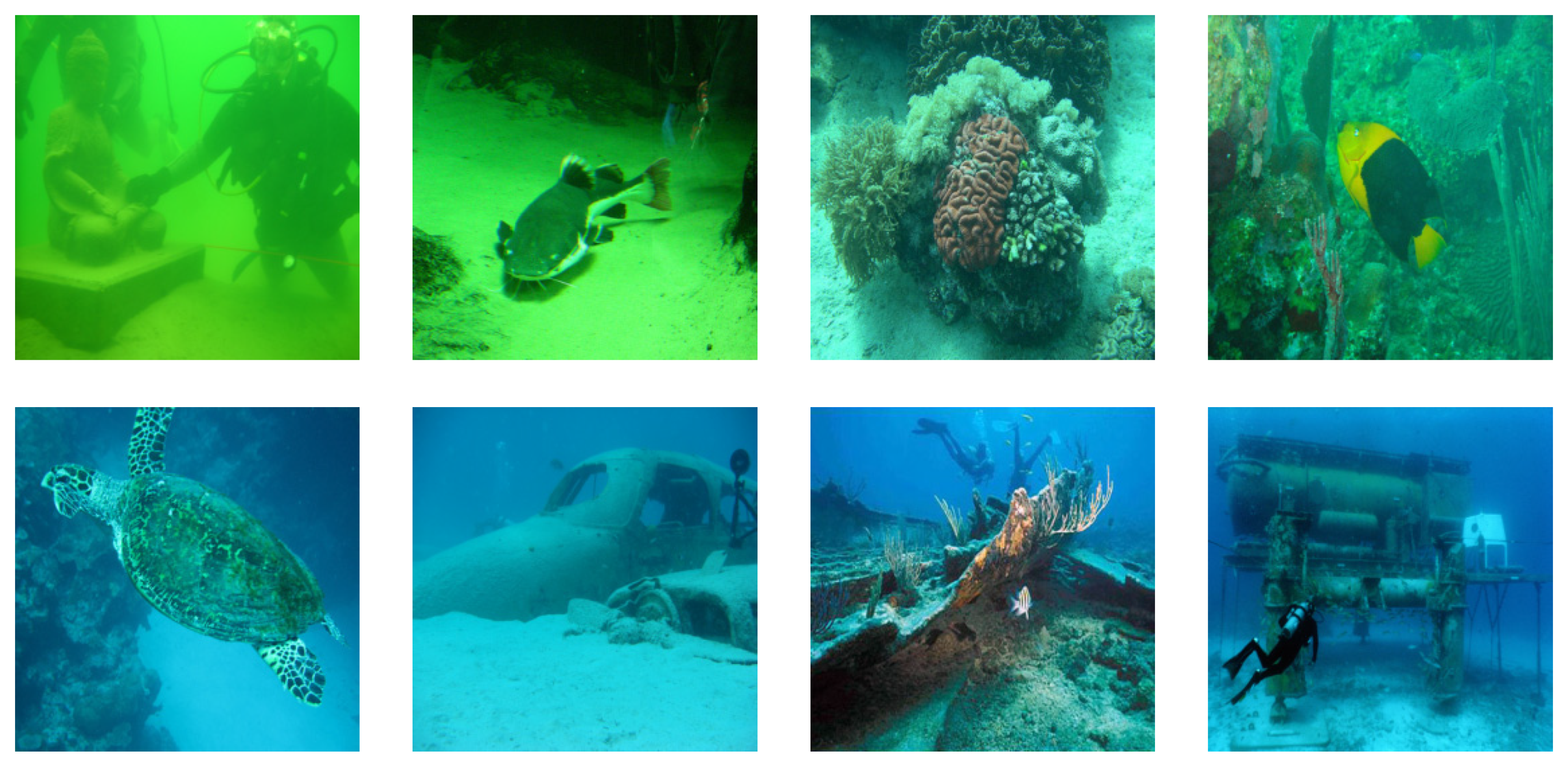
Figure 1.
Real underwater images were collected in the UIQE database.
Figure 1.
Real underwater images were collected in the UIQE database.
Figure 2.
The effects of 9 different methods on underwater image enhancement are shown. (a) Raw. (b) CycleGAN. (c) FGAN. (d) RB. (e) RED. (f) UDCP. (g) UGAN. (h) UIBLA. (i) UWCNN-SD. (j) WSCT.
Figure 2.
The effects of 9 different methods on underwater image enhancement are shown. (a) Raw. (b) CycleGAN. (c) FGAN. (d) RB. (e) RED. (f) UDCP. (g) UGAN. (h) UIBLA. (i) UWCNN-SD. (j) WSCT.
Figure 3.
Comparison of mean and standard deviation of MOS values of different enhancement algorithms.
Figure 3.
Comparison of mean and standard deviation of MOS values of different enhancement algorithms.
Figure 4.
The effects of 9 different methods on underwater image enhancement are shown.
Figure 4.
The effects of 9 different methods on underwater image enhancement are shown.
Figure 5.
GM map of different enhancement methods. (a) the original image, (b) the GM map on the original image, (c) the UDCP map, (d) the GM map on the UDCP map, (e) the UBCP map and (f) the GM map on the UBCP map. The first line represents CycleGAN, the second line represents FGAN, the third line represents RB, the fourth line represents RED, the fifth line represents UDCP, the sixth line represents UGAN, the seventh line represents UIBLA, the eighth line represents UWCNN-SD, and the ninth line represents WSCT.
Figure 6.
LOG map of different enhancement methods. (a) the original image, (b) the LOG map on the original image, (c) the UDCP map, (d) the LOG map on the UDCP map, (e) the UBCP map and (f) the LOG map on the UBCP map. The first line represents CycleGAN, the second line represents FGAN, the third line represents RB, the fourth line represents RED, the fifth line represents UDCP, the sixth line represents UGAN, the seventh line represents UIBLA, the eighth line represents UWCNN-SD, and the ninth line represents WSCT.
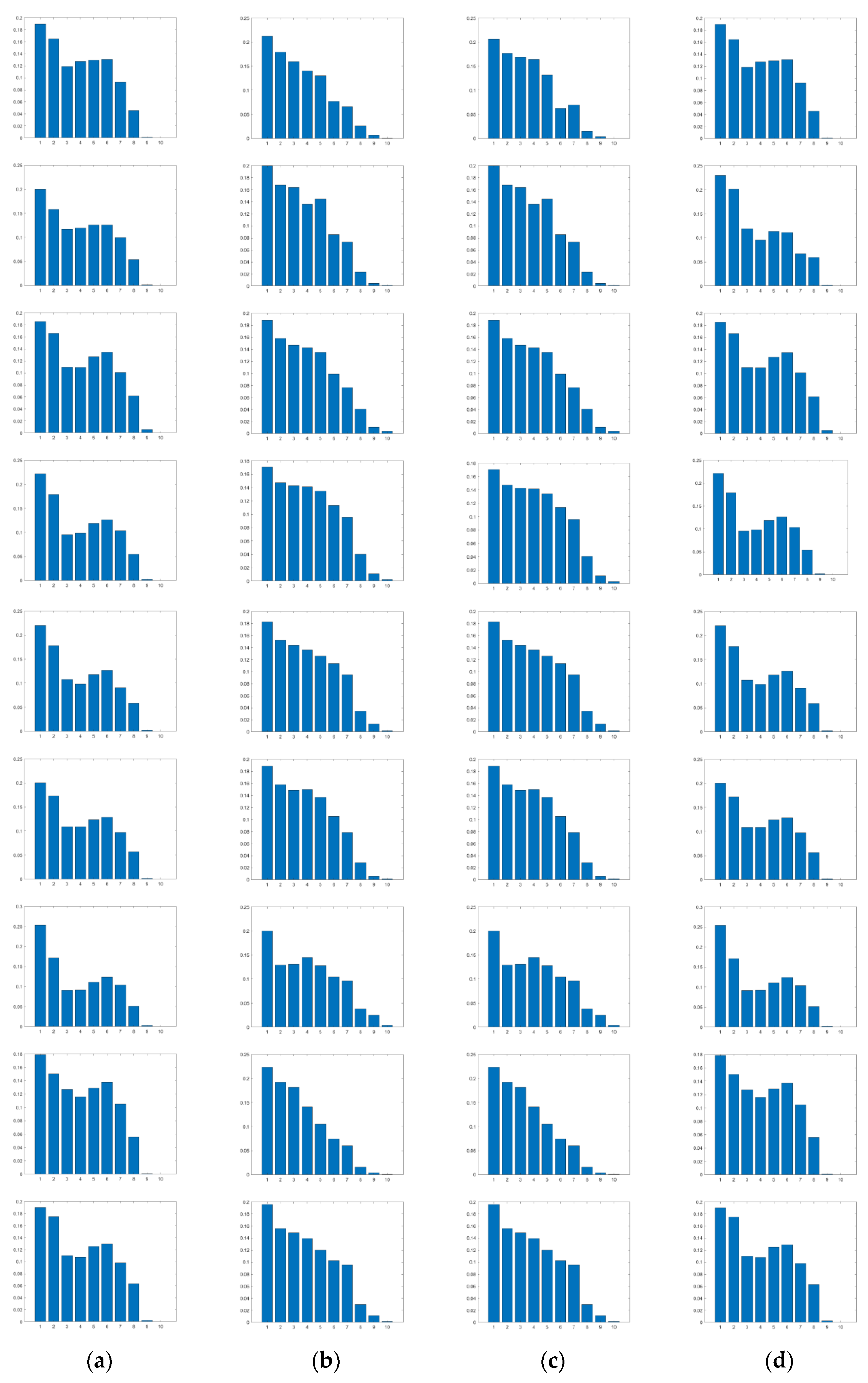
Figure 7.
Marginal probabilities between normalized GM and LOG features for images of the UDCP maps and the UBCP maps. (a) Histogram of PG on UBCP, (b) Histogram of PL on UBCP, (c) Histogram of PG on UBCP, (d) Histogram of PL on UDCP. The abscissa indicates that the feature is divided into 10 dimensions, and the ordinate indicates the sum of marginal distribution. The first line represents CycleGAN, the second line represents FGAN, the third line represents RB, the fourth line represents RED, the fifth line represents UDCP, the sixth line represents UGAN, the seventh line represents UIBLA, the eighth line represents UWCNN-SD, and the ninth line represents WSCT.
Figure 8.
Independency distribution between normalized GM and LOG features for images of UBCP. (a) Histogram of QG on UBCP, (b) Histogram of QL on UBCP, (c) Histogram of QG on UBCP, (d) Histogram of QL on UDCP. The abscissa indicates that the feature is divided into 10 dimensions, and the ordinate indicates the sum of conditional distribution. The first line represents CycleGAN, the second line represents FGAN, the third line represents RB, the fourth line represents RED, the fifth line represents UDCP, the sixth line represents UGAN, the seventh line represents UIBLA, the eighth line represents UWCNN-SD, and the ninth line represents WSCT.
Figure 9.
SROCC values of different dimensions M = N = {5, 10, 15, 20} in the database.
Figure 9.
SROCC values of different dimensions M = N = {5, 10, 15, 20} in the database.
Figure 10.
Comparison of the performance of BRSIQUE, NIQE, UCIQE, UIQM, CCF, ILNIQE and UIQEI in three scenes. (a) in blue scene, (b) in green scene, (c) in haze scene.
Figure 10.
Comparison of the performance of BRSIQUE, NIQE, UCIQE, UIQM, CCF, ILNIQE and UIQEI in three scenes. (a) in blue scene, (b) in green scene, (c) in haze scene.
Figure 11.
The performance of a class of features (SROCC and PLCC) in the UIQE database. f1–f84 are the feature IDS given in
Table 2.
Figure 11.
The performance of a class of features (SROCC and PLCC) in the UIQE database. f1–f84 are the feature IDS given in
Table 2.
Table 1.
Rating analysis of underwater image enhancement.
Table 1.
Rating analysis of underwater image enhancement.
| Range | Describe |
|---|
| 1 | No color recovery, low contrast, texture distortion, edge artifacts, poor visibility. |
| 2 | Partial color restoration, improved contrast, texture distortion, edge artifacts, and poor visibility. |
| 3 | Color recovery, contrast enhancement, realistic texture, local edge artifacts, and acceptable visibility. |
| 4 | Color recovery, contrast enhancement, texture reality, better edge artifact recovery, and better visibility. |
| 5 | Color restoration, contrast enhancement, texture reality, edge artifacts, and good visibility of underwater images. |
Table 2.
Summary of 84 extracted features.
Table 2.
Summary of 84 extracted features.
| Index | Feature Type | Symbol | Feature Description | Feature ID |
|---|
| 1 | GM and LOG of the underwater dark channel map | PG, PL, QG, QL | Measure the local contrast of the image | |
| 2 | GM and LOG of the underwater bright channel map | PG, PL, QG, QL | Measure the local contrast of the image | |
| 3 | Color | Isaturation(i, j), CF | Measure the color of the image | |
| 4 | Fog density | D | Measure the fog density of the image | |
| 5 | Global contrast | GCF | Measure the global contrast of the image | |
Table 3.
Performance comparison of BRSIQUE, NIQE, UCIQE, UIQM, CCF, ILNIQE and UIQEI methods.
Table 3.
Performance comparison of BRSIQUE, NIQE, UCIQE, UIQM, CCF, ILNIQE and UIQEI methods.
| | SROCC | PLCC | RMSE |
|---|
| BRSIQUE [50] | 0.5495 | 0.5446 | 0.6188 |
| NIQE [51] | 0.3850 | 0.4079 | 0.6736 |
| UCIQE [22] | 0.2680 | 0.3666 | 0.6864 |
| UIQM [23] | 0.5755 | 0.5898 | 0.5958 |
| CCF [24] | 0.2680 | 0.3666 | 0.6864 |
| ILNIQE [52] | 0.1591 | 0.1749 | 0.7264 |
| UIQEI | 0.8568 | 0.8705 | 0.3600 |
Table 4.
Different feature groups.
Table 4.
Different feature groups.
| Index | Feature |
|---|
| G1 | GM under UBCP |
| G2 | LOG under UBCP |
| G3 | GM under UDCP |
| G4 | LOG under UDCP |
| G5 | Color feature |
| G6 | Fog density feature |
| G7 | Global contrast feature |
| G8 | Excluding the global contrast feature |
Table 5.
Performances of different groups.
Table 5.
Performances of different groups.
| | SROCC | PLCC | RMSE |
|---|
| G1 | 0.7850 | 0.8029 | 0.4359 |
| G2 | 0.7742 | 0.8001 | 0.4381 |
| G3 | 0.8134 | 0.8211 | 0.4184 |
| G4 | 0.8085 | 0.8193 | 0.4196 |
| G5 | 0.6360 | 0.7519 | 0.4825 |
| G6 | 0.7304 | 0.7849 | 0.4552 |
| G7 | 0.3981 | 0.4438 | 0.6579 |
| G8 | 0.8455 | 0.8603 | 0.3714 |
Table 6.
Performance under different training test split.
Table 6.
Performance under different training test split.
| Train-Test | SROCC | PLCC | RMSE |
|---|
| 80–20% | 0.8568 | 0.8705 | 0.3600 |
| 70–30% | 0.8494 | 0.8605 | 0.3736 |
| 60–40% | 0.8433 | 0.8528 | 0.3841 |
| 50–50% | 0.8313 | 0.8424 | 0.3965 |
| 40–60% | 0.8157 | 0.8282 | 0.4120 |
| 30–70% | 0.7941 | 0.8115 | 0.4315 |
| 20–80% | 0.7845 | 0.7833 | 0.4576 |


