A Fast Circle Detector with Efficient Arc Extraction

Abstract

Circle detection is a crucial problem in computer vision and pattern recognition. Improving the accuracy and efficiency of circle detectors has important scientific significance and excellent application value. In this paper, we propose a circle detection method with efficient arc extraction. In order to reduce edge redundancy and eliminate crossing points, we present an edge refinement algorithm to refine the edges into single-pixel-wide branchless contour curves. To address the contour curve segmentation difficulty, we improved the CTAR (Chord to Triangular Arms Ratio) corner detection method to enhance corner point detection and segment the contour curves based on corner points. Then, we used the relative position constraint of arcs to improve the circle detection accuracy further. Finally, we verified the feasibility and reliability of the proposed method by comparing our approach with five other methods using three datasets. The experimental results showed that the presented method had the advantages of anti-obscuration, anti-defect, and real-time performance over other methods.

1. Introduction

Shape analysis is a crucial problem in image processing and computer vision. Circles, as one of the simplest shapes in our daily life, have attracted the attention of many researchers. In the past decades, circle detection has been applied in various scenarios, such as cell segmentation [1,2,3], PCB hole detection [4,5], ring traffic sign detection [6,7], spacecraft attitude analysis [8,9], iris detection [10,11,12], and ball detection [13,14]. The demand for circle detection accuracy and efficiency continues to increase as these usage scenarios change. However, many circle detection methods fail because of complex backgrounds, noise, occlusions, and defects. As pointed out in [15], these solutions are far from satisfactory compared to human perception.

Early classical circle detection methods were based on Circle Hough Transform (CHT) [16,17]. These methods search circles by mapping 2D coordinates to 3D coordinates. Any three points on the edge are mapped to a point in 3D space, and this point represents a circle. Then, the candidate circles are determined by voting for these points. CHT-based circle detectors have to traverse and iterate over a large number of edge points, so such detectors are time-consuming. Moreover, these methods are more susceptible to interference from noise, which leads to a decrease in accuracy. Some researchers corrected the shortcomings of the noise resistance of CHT by hypothesis filtering [18]. However, there is still a problem of long processing time, though its accuracy is better. Xu et al. [19] proposed Randomized Hough transform (RHT). This method does not completely traverse all of the edge points, but samples them for processing, which greatly reduces the processing time. Later methods, such as curvature-aided HT (CACD) [20], also use RHT to detect circles with good results. Unfortunately, the generation of candidate circles in complex backgrounds or noisy scenes still requires several attempts. Su et al. [21] improved the operation speed by reducing the redundant computation of voting through a min/max voting approach and a sparse structure for batch computation. However, the efficiency decreases rapidly once it is interfered with by noise, similar to other CHT-based methods.

Unlike the CHT-based methods with complete traversal at the edge, RCD [22] uses four points randomly sampled in each iteration. Three of the points determine a circle, and the fourth point is used to check the compatibility of the circle. Although the detection speed is improved compared to CHT-based methods, it still requires more iterations to generate candidate circles, because the probability that the sampled points are from the same circle is small, especially in the case of more noise. Chung et al. [23] improved RCD by efficient sampling and using refinement strategies to obtain lower time consumption and higher accuracy. Although the precision, recall, and time consumption of these RCD-based methods have improved, they are still far from real-time detection.

The main reason why CHT-based and RCD-based methods are time-consuming is the large number of iterations and traversal computations. To solve this problem, another type of method uses the geometric properties of circles to perform detection. These methods extract the arcs first and then estimate the circle parameters by least-squares circle fitting, circle-inscribed triangles, or perpendicular bisector intersections. The key to these methods based on geometric properties is extracting the arc efficiently and accurately. Le et al. [24] used a line segment detector [25] to extract the circular curve and then performed least-squares circle fitting to obtain the circle parameters. Although this method achieved good performance, there was the problem of useless least-squares fitting and redundant calculations caused by straight lines. This causes the detection time to become longer. Akinlar et al. [26] proposed an approach based on Edge Drawing Parameter Free (EDPF) [27,28,29]. They converted the edge into line segments and converted the line segments into arcs. Then, they estimate circle parameters by continuously calling least-squares circle fitting, where arcs with similar circle parameters were clustered together. However, a significant deviation occurs when the circle has defects or occlusions. On the basis of EDPF, Zhao et al. [30] constrained arcs of the same circle by estimating the circle parameters using the inscribed triangle. It takes advantage of the fact that area calculation is more robust to noise [31], which significantly improves the accuracy of circle detection. The circle parameters estimation method has equivalent accuracy to the least-squares fitting method because they also used a linear error compensation algorithm to exact circle parameters, which was not faster than that of least-squares fitting. Lu et al. [32] determined whether the curve is an initial circle using the criterion of area restriction, radius, gradient polarity analysis, and inside diameter. Then, the initial circles were clustered to generate candidate circles. This was more accurate in complete circles, but often failed to identify occluded circles. The common problem with these methods is that their detection speed is far from real-time as they have more redundant computations.

There are other approaches. Dasgupta et al. [33] proposed a population intelligence technique with adaptive bacterial foraging optimization for circle detection. This method was more sensitive to noise, though it could produce better results on images with clean backgrounds. Ayala-Ramirez et al. [34] proposed a genetic algorithm for circle detection, and the method also failed in detecting circles with defects or occlusions. Moreover, these methods have the same disadvantage of having prolonged time consumption.

To improve the accuracy and time efficiency of circle detection, we removed the redundant pixels and split out the useless contour curves. Candidate circle parameters were derived using least-squares circle fitting, and the relative position constraints of the arcs were added to improve the circle detection accuracy. Finally, genuine circles were extracted by a rigorous candidate circle validation. The main contributions of this paper are

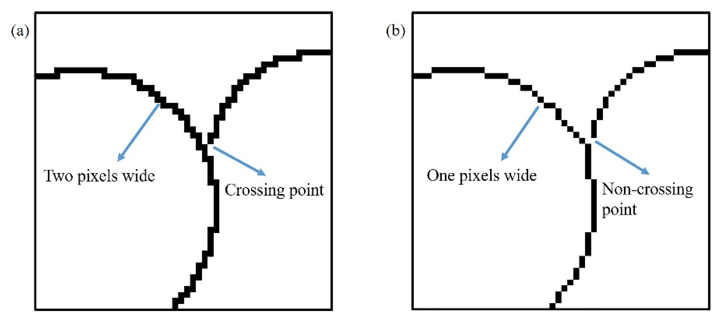
• A method of image edge refinement that reduces edge redundancy while effectively eliminating intersections;
• An improved CTAR [35] corner-detection algorithm that ensures complete corner detection of contour curves by adding positive–negative point detection, adaptive sampling interval, and adaptive thresholds;
• One complete circle dataset and one incomplete circle dataset are constructed, and the circle detection algorithm was fully tested on these datasets.

The steps of the proposed method are given in Section 2. Section 3 reports the experimental results and provides a comparative analysis. Section 4 concludes this paper.

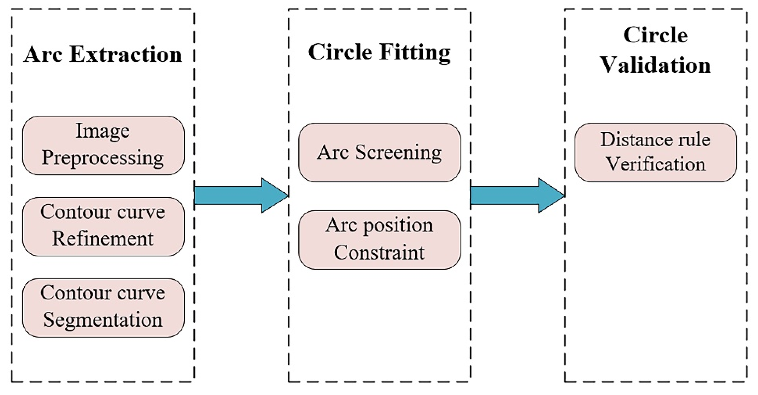
2. Methodology

Given an image, the circle detection steps of our proposed method are shown in Figure 1. A detailed description of the framework is presented in the following.

2.1. Arc Extraction

2.1.1. Image Preprocessing

The purpose of image preprocessing is to reduce the image noise and extract edges. We used a 5 × 5 median filter to reduce the noise. Then, we adopted the Canny [36,37] edge detector to obtain contour curves, as used by most circle detectors. Figure 2a shows a test image, and Figure 2b shows its contour curves.

2.1.2. Contour Curve Refinement

The contour curves were multiple pixels wide, because Canny evaluated the pixels in an isolated manner to extract edges [29]. These curves contained many crossing points. Figure 3a shows a simple case. A one-pixel-wide contour curve can accurately describe a circle, while multi-pixel-wide curves will lead to computational redundancy. Therefore, the multi-branched contour curves with crossing points needed to be transformed into non-branched contour curves to facilitate the extraction of the arc. Deleting redundant pixels and crossing points can solve the two problems, as shown in Figure 3b.

Point P is deleted from the contour curve if it satisfies any one of the following conditions:

$$N(1)N(3)+N(3)N(5)+N(5)N(7)+N(7)N(1)=true\hspace{0.17em}\&\hspace{0.17em}N(P)=2,$$

(1)

$$(N(1)+N(5))(N(3)+N(7))=true\hspace{0.17em}\&\hspace{0.17em}N(P)>2,$$

(2)

$$N(1)N(4)N(6)+N(3)N(6)N(8)+N(2)N(5)N(8)+N(2)N(4)N(7)=true\hspace{0.17em},$$

(3)

$$Nc(P)>2\hspace{0.17em}.$$

(4)

where N(p) is the number of foreground points in the eight-neighbor of P, N(1~8) is the eight-neighbor of P, as shown in Figure 4, and N_c(P) is the number of foreground pixels in N(2), N(4), N(6), and N(8). We specified that the contour curve pixel logical value is 1 (true), and the background pixel logical value is 0 (false). Conditions (1)–(4) should be applied in a logical order. The part without pixels is treated as background pixels when P is on the image’s border. The effect of contour curve refinement is shown in Figure 2c.

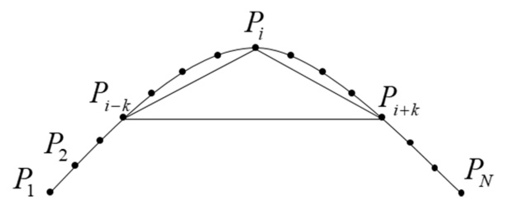
2.1.3. Contour Curve Segmentation

To speed up the subsequent process, similar to Jia et al. [38], contour curves with less than 25 pixels are removed, regardless of the image resolution. After that, the image contains four kinds of contour curves: single arc, interference curves, curves with multiple arcs, and a combination of arc and interference curves. As shown in Figure 5, except for the single arc, the other three curves include several corner points distributed at the intersection of arcs, the intersection of arcs and interference curves, and the intersection of interference curves.

The curves shown in Figure 5c,d can be transformed into arcs and interfering contour curves by dividing them at the corner points. Here, we addressed the CTAR [35] corner detector to improve the corner detection capability when used for circle detection. The original CTAR estimates the curvature of point P_i, as shown in Figure 6, based on

$$R(P_i)=\frac{{\Vert P_{i+k}-P_{i-k}\Vert }_2}{{\Vert P_i-P_{i-k}\Vert }_2+{\Vert P_{i+k}-P_i\Vert }_2},$$

(5)

where P_i+k is the point reached by traversing k points in the positive direction from P_i and P_i−k is the point reached by traversing k points in the negative direction from P_i.

The value of k and the corner points determination threshold are fixed in CTAR. The point is determined as a corner point when k = 3 and R(P_i) < 0.989. However, a fixed k and fixed threshold do not detect very well due to the complex contour curve. To solve this problem, we used auto-adaptive k and the corner threshold, positive–negative point determination, large-scale coarse localization, and small-scale fine localization to enhance the accuracy of the CTAR.

Considering the demand for subsequent adaptive threshold setting, we modified Equation (5) as follows:

$$R(P_i)=\frac{{\Vert P_i-P_{i-k}\Vert }_2+{\Vert P_{i+k}-P_i\Vert }_2}{{\Vert P_{i+k}-P_{i-k}\Vert }_2}.$$

(6)

Adjusting Equation (5) does not change the detection performance. All of the k values in different contour curves are different. k is determined by the curve length and the image size. As shown in Equation (7), for the calculation of k:

$$k=\eta \times (\frac{S}{100}+3)+(1-\eta )\times (\frac{\min (width,height)\times \pi }{100}+3),$$

(7)

where 0 ≤ η ≤ 1 is the weight parameter, S is the length of the curve, and $\min (width,height)$ is the smaller value of the image length and image width. Equation (7) limits k to a minimum of 3, which is the same as the fixed sampling interval of CTAR. In order to balance the impacts of curve length and image size on k, η is set to adjust the weights to accommodate different types of images.

The curvature set $R$ of a curve is obtained by Equation (8). Mean plus or subtract two standard deviations are based on the typical distribution characteristics, where 95.44% of the data appear in this range [39]. Therefore, using the mean curvature plus two standard deviations as a threshold can judge corner points. Therefore, the corner point threshold is calculated based on

$$T_c=\overline{R}+2\sqrt{\frac{{\displaystyle \sum _{i=1}^n{(R_i-\overline{R})}^2}}{n}}$$

(8)

where $\overline{R}$ is the mean of $R$. Points with curvature greater than T_c are determined to be corner points and form the set $C_1$.

According to Equation (7), k will be larger when a contour curve has multiple arcs, as shown in Figure 5c. Since a larger k value will smooth the curve, it makes the corner points among the arcs remain undetected. It is more likely to occur when the curvature of the corner points is similar to that of the arc. Therefore, we introduce the positive–negative point detection scheme [40] to improve the corner detection ability. As shown in Figure 7, line l_i is formed by P_i−k and P_i. The relative position of P_i+k and l_i is used to determine the symbol of P_i. P_i+k is defined as a positive point when P_i+k is in the clockwise rotation direction of l_i or on l_i. The symbol of P_i is set as ‘+’ when P_i+k is a positive point. Figure 7 shows the four positive point cases. Similarly, it is defined as a negative point when P_i+k is in the counterclockwise direction of l_i, and the symbol of P_i is ‘−’.

According to the definition of positive and negative points, we used

$$s_{P_i}=\{\begin{array}{l}+, (x_{P_i}-x_{P_{i-k}})\times (y_{P_{i+k}}-y_{P_{i-k}})+(y_{P_{i-k}}-y_{P_i})\times (x_{P_{i+k}}-x_{P_{i-k}})<=0\\ -, (x_{P_i}-x_{P_{i-k}})\times (y_{P_{i+k}}-y_{P_{i-k}})+(y_{P_{i-k}}-y_{P_i})\times (x_{P_{i+k}}-x_{P_{i-k}})>0\end{array}$$

(9)

to determine the symbol of $P_i$. A sequence of symbols was obtained after traversing the entire curve. Then, we performed the same window smoothing operation twice for the symbol sequence to reduce the noise.

For the analysis of contour curves shown in Figure 2c, there were only a small number of corner points on these curves. A curve had a high number of positive or negative points, and corners existed in the region where a smaller number of symbol points were located. These points with a smaller number of symbols are called support points. Each section of consecutive support points is called the support area, as shown in Figure 8. For each support area, set k to 3 to finely locate the corner points. The point with the largest R(P_i) in the support area was determined as the corner point and formed set $C_2$.

Then, the contour curve was segmented according to $C_1$ and $C_2$. In summary, each contour curve segmentation was carried out in the following steps.

(a)

Calculate k according to Equation (7);

(b)

The curvature of the point on the curve is estimated;

(c)

Calculate T_c based on Equation (8);

(d)

Derive the corner set $C_1$ based on T_c;

(e)

Positive–negative point detection, sliding window filtering of positive–negative point sequence, and statistical support area determination;

(f)

The curvature is estimated by k = 3 in the support area, and the maximum curvature point of each support area is the corner point; thus, $C_2$ is derived;

(g)

Split the curve according to $C_1$ and $C_2$.

If the original CTAR corner point detection method is followed, then steps (a), (c), (e), and (f) above are not needed. In this paper, we improved CTAR corner point detection by adding steps (a), (c), (e), and (f). Algorithm 1 shows the whole contour curve segmentation process. The new contour curves for Figure 2c are shown in Figure 2d, and each contour curve is shown with different colors.

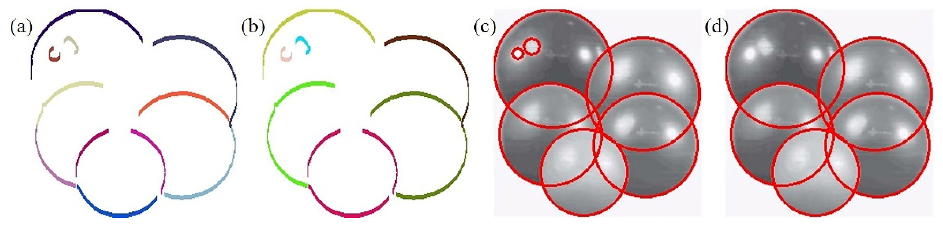
2.2. Circle Fitting

2.2.1. Arc Screening

Contour curves with less than 25 pixels are removed, as in Section 2.1.3. Curves whose ratio of arc length to circumference is greater than τ are used to fit the circle. It can easily deduce that, when the curve length is constant, the straighter the curve is, the smaller the ratio. Thus, we defined a curve whose ratio was below or equal to τ, was a straight line, and did not participate in circle fitting. τ was set to 0.2 in the proposed method, and the analysis of the choice is given in Section 3.3.2. See Figure 9a for reference; it should satisfy α > 72° when the ratio of arc length to the circumference is greater than 0.2. We took line L₁ and line L₂ to calculate θ. L₁ was formed by the starting point $P_s$ and the midpoint P_m of the curve. L₂ was formed by the midpoint P_m and the endpoint P_e. θ was 0.5 times α according to the simple principle of geometry. Therefore, it was calculated that θ should be greater than 36°.

Algorithm 1 Contour Curve Segmentation
Input: Curve set $\Psi =\{c_1,c_2,\dots ,c_n\}$
Output: Curve group set $\Theta$
1   Initialize parameters
2   while $\Psi \ne \varnothing$ do
3		for $c_i\in \Psi$ do
4			Initialize curvature set $C_R\leftarrow \varnothing$
5			Initialize direction set $D\leftarrow \varnothing$
6			Initialize corner set $C\leftarrow \varnothing$
7			Calculate $k$ by Equation (7) and then limit the maximum value to 15
8			for $P\in c_i$ do
9				Calculate $R$ by Equation (6) and then push it in $C_R$
10				Calculate $S$ by Equation (9) and then push its coordinate in $D$
11			end for
12			Twice smoothed the $D$
13			Obtain the set of support area $H$ form $D$
14			Set $k=2$
15			Initialize $C_2\leftarrow \varnothing$
16			for $c_n\in H$ do
17				Initialize $C_H\leftarrow \varnothing$
18				for $P\in c_n$ do
19					Calculate R by Equation (6) and then push it in CH
20				end for
21				Find the maximum value in CH and then push its coordinate in C2
22			end for
23			Calculate corner threshold Tc by Equation (8)
24			Initialize $C_1\leftarrow \varnothing$
25			for $P\in C_R$ do
26				if $P>T_c$ then
27					Push coordinate of P in C1
28				end if
29			end for
30			Push the set of curves obtained by dividing $c_i$ by C1 and C2 into $\Theta$
31		end for
32	end while
33   Return

For Figure 9b, when the arc occupies a more significant proportion, it may also cause θ ≤ 36°. In this case, we chose the difference between ${\Vert P_m-P_s\Vert }_2+{\Vert P_e-P_m\Vert }_2$ and ${\Vert P_e-P_s\Vert }_2$ to judge whether the curve was a straight line. Since ${\Vert P_m-P_s\Vert }_2\approx {\Vert P_e-P_m\Vert }_2$, the problem can be expressed to

$$\begin{array}{l}minimize\hspace{0.17em}\hspace{0.17em}\hspace{0.17em}\xi =2{\Vert P_m-P_s\Vert }_2-{\Vert P_e-P_s\Vert }_2=2{\Vert P_s-P_m\Vert }_2(1-\sin \frac{\theta }{2})\\ subject\hspace{0.17em}to\hspace{0.17em}\hspace{0.17em}\theta \le 36°\end{array}$$

(10)

We obtained ${\xi }_{\min }=1.38{\Vert P_s-P_m\Vert }_2$ according to a simple calculation. Therefore, if $\xi \le 1.38{\Vert P_s-P_m\Vert }_2$, the curve was judged to be a straight line.

In conclusion, only curves that satisfy either condition θ ≤ 36° or $\xi >1.38{\Vert P_s-P_m\Vert }_2$ can be fitted to the circle. Figure 10a shows the result after contour curve screening.

2.2.2. Arc Relative Position Constraint

KASA circle fitting [41] is one of the implementations of least-squares circle fitting. We estimated the circle parameters (x, y, r) for each curve by KASA, where (x, y) is the circle center, and r is the radius. We selected the fitted points by equally spaced sampling on the curve to improve the fitting speed. The sampling interval was determined by

$$n=S/50+1$$

where S is the curve length. An initial circle set can be obtained by KASA.

We considered two circles to be congruent when circle i and circle j have at least 80% overlap, as suggested by Jia et al. [38], Zhao et al. [30], and Lu et al. [32]. We defined the overlap ratio between C_i and C_j in the following manner:

$$Overlap Ratio(C_i,C_j)=\frac{area(C_i)\cap area(C_j)}{area(C_j)\cup area(C_j)},$$

(11)

where $area(C_{*})$ denotes the area of $C_{*}$. When $Overlap Ratio(C_i,C_j)>=0.8$, curves i and j are on the same circle. Then, the two curves are combined into one curve. The same is true for the operation of multiple curves on the same circle.

Different curves on the same circle are constrained to one curve, which improves the accuracy of circle detection. KASA with equally spaced sampling is then performed for each combined curve. We labeled the curves on the same circle with the same color in Figure 10b.

2.3. Circle Validation

Identifying the true or false of the fitting circles is a crucial process to improve the accuracy of circle detection. Figure 10c shows an image containing the two error circles. The distribution of points on the wrong circle curve was very different from the distribution of points on the correct circle curve. We reflected it in the standard deviation of the distance between points on the curve and the center of the fitted circle. It was quickly concluded that the standard deviation of the interference curve was much larger than that of the arc. To simplify the calculation, we replaced the standard deviation with the sum of absolute values of l_i − r. l_i is a line segment from P_i to circle center O. l_i − r is shown in Figure 11.

A true or false circle is defined as follows:

$$circle=\{\begin{array}{l}true,{\displaystyle \sum _{i=1}^S\left|l_i-r\right|\hspace{0.17em}<\hspace{0.17em}\lambda rS}\\ false,{\displaystyle \sum _{i=1}^S\left|l_i-r\right|\hspace{0.17em}\ge \hspace{0.17em}\lambda rS}\end{array},$$

(12)

where S is the length of the curve and λ is the allowable curve deviation degree coefficient. The smaller the λ, the tighter the circle verification. The final circle detection result for Figure 2a is shown in Figure 10d.

3. Experimental

This section shows the results of the proposed method on many datasets and compares them with the results of other methods. Furthermore, all experiments were performed on an Intel Core i5-9400 2.9 GHz desktop with 8 G RAM.

3.1. Performance Metrics

We used the average detection time and three well-known metrics in the information retrieval area to assess the proposed method: precision, recall, and F-measure. Except for the average detection time, the other metrics are defined as $precision=\frac{TPs}{TPs+FPs}$, $recall=\frac{TPs}{TPs+FNs}$, and $F-measure=\frac{2\times precision\times recall}{precision+recall}$, where $TPs$ is the number of correct predictions, $FPs$ is the number of incorrect predictions, and $FNs$ is the number of omissions. All three indicators are within the range [0, 1].

According to the expressions of precision and recall, we can learn that precision evaluates the percentage of correct circles among the detected circles, while recall indicates the percentage of correctly detected circles among all ground truth circles. We would certainly like to have greater precision and recall, but the two are contradictory in most cases. For example, given an image containing multiple circles, in the extreme case, only one circle is detected and it is true. Therefore, the precision is 1, but the recall is low. If we detect all circles, but more false circles, then the recall is 1 and the precision is very low. A single precision or recall metric does not directly reflect the strength of the detector. The F-measure was generated to consider these two metrics, which reflected the overall detection performance. The larger the F-measure, the better the detection effect.

We considered the detected circle correct when the detected circle had at least 80% overlap with the ground truth circle. It was the same definition as that in Section 2.2.2 for two circles being the same circle.

3.2. Dataset

We performed experiments using three datasets, which were used to analyze the performance of the circle detector for complete circles and circles with occlusions. Additionally, the size of all images was less than 1000 × 1000.

Mini. For this dataset, eight common images were used to test circle detectors over the years [26,42,43,44], as shown in Figure 12: Stability-ball (236 × 236 pixels), Coin (256 × 256), Plates (400 × 390), Cake (231 × 231), Ball (231 × 232), Gobang (239 × 237), Swatch (236 × 272), and Insulator (204 × 150).

Complete-circle. This included 183 images that contained different scenes. These images were obtained from [30,32], and the internet. Some of the PCB images inside contained different noise levels. As a result, more circles were included in each image, and the background was more complex. Some images may have had near-elliptical circles because the camera view was not perfectly perpendicular to the scene. Nevertheless, all the circles in this dataset were complete circles with no defects and no occlusions.

Incomplete-circle. This also included 125 images, such as eyes, balls, plates, and cartoon images. The sources of the images were the same as those of the Complete-circle dataset. Unlike the Complete-circle dataset, the images in this dataset contained some circles with defects or obscurities, making detection more difficult.

3.3. Method Analysis

3.3.1. Ablative Analysis

To test the performance of the improved CTAR corner detector, we conducted a comparison experiment with the original CTAR. We added Gaussian noise with zero mean and 1–12% variance to the images separately to test the robustness. The experimental results are shown in Figure 13. The results showed that many non-corners were also detected as corners, because the original CTAR used fixed sampling intervals and a fixed corner point threshold. Although the detection could be improved by modifying these two parameters, the radius of the circle was not equal on each image, which needed to use different parameters for different images to achieve better results. Even in the same image, the radii of the different circles were not equal.

In contrast, the sampling interval and corner point threshold of our improved CTAR was different for each curve. It effectively reduced the detection error of corners. The smoothness of the contour curve decreased as the noise increased, and the original CTAR became more sensitive. Therefore, the result was that the curves retained after curve splitting and filtering became sparser, which led to a smaller number of correct circles in the end. In comparison, the improved CTAR algorithm had higher anti-interference performance and more robust adaptability.

We also used the same images as in Figure 13 to perform experiments on the relative position constraint. The experimental results are shown in Figure 14. We used the colors in the second and third rows to distinguish the curves on different circles, and curves on the same circle were identified with the same color. Curves without color were considered invalid curves. The quantitative analysis is shown in Figure 15. The results show that the relative position constraint effectively improved the detection. Because it constrained the curves on the same circle to one curve, this increased the number of points involved in KASA circle fitting; i.e., it improved the precision of the circle fitting. The recall with and without the relative position constraint had smaller difference. Therefore, from the comprehensive performance F-measure, the experimental results after the relative position constraint were better than those without the relative position constraint.

The projection distortion may cause the circle to take on an elliptical shape. Therefore, we also tested whether the proposed method could detect ellipse-like circles. We selected ellipse images with eccentricity e from 0 to 0.54 for the experiment, as shown in the first row of Figure 16. The results are shown in the second row. The results show that our method can accept ellipses with e ≤ 0.47 as circles. This condition is limited by the λ of circle validation in Equation (12). We can accept larger e by slightly increasing λ. However, as the eccentricity increased, the detected circle was also more off the ellipse’s center, and the precision decreased rapidly. Therefore, our method was more suitable for cases where the degree of distortion is not very large.

3.3.2. Threshold Analysis

There were three parameters in the proposed method, namely η, τ, and λ. Due to the complexity of the images, it was not possible to obtain the best results for each image with a fixed set of parameters. In order to reveal the effect of these three parameters on the proposed method, a series of experiments for the F-measure were conducted. We conducted experiments for each parameter separately using the control variable method.

In the curve segmentation stage, η was used to determine how much the sampling interval was affected by the curve length and the image size, and a larger η indicated that the sampling interval was more affected by the curve length. Figure 17a shows that better results could be obtained when η = 0.7 or 0.8. The Mini and Complete-circle datasets had the highest F-measure when η = 0.7, and only the Incomplete-circle dataset had the highest F-measure when η = 0.8. Therefore, we chose to use η = 0.7. We used τ to determine whether a curve was a straight line or not. As τ increased, more curves were judged to be straight lines. The highest F-measure was found on all three datasets when τ = 0.2 according to Figure 17b. Therefore, τ was set to 0.2. λ was used to determine the true and false circles in the circle verification stage, and a smaller value indicated more stringent circle verification. From Figure 17c, the best results were obtained when λ = 0.06. Therefore, λ was set to 0.06 in the proposed method.

3.4. Performance Comparison

On the three datasets, the proposed method was compared with several methods: the four-point random sampling-based method RCD [22], the geometry-based method EDCircles [26] with pseudo circle detection control, the improved RHT-based method CACD [20], the AS method [32] with arc-supported line segments, and Zhao M Y’s [30] method using inscribed triangles. All comparison methods are available and open-source on the Internet. Note that, regarding the application of the circle detectors, we considered all of the parameters as default parameters. These parameters were set only once and then kept constant in all of the experiments reported below. The parameters of our method were set to η = 0.7, τ = 0.2, λ =0.06. On the other hand, we used the default parameters from the other methods to obtain the initial detection results. These parameters were the better ones illustrated in the literature on these methods. For example, for CACD, we set the number of iterations to 60,000, as described in the literature [20]. Meanwhile, the CACD and AS methods were run in Matlab R2018b, and the other three methods and our method were run in VS2019.

For the Mini dataset, the detection time is shown in

Table 1. Time consumption of the Mini dataset.

Images	RCD	EDCircles	CACD	AS	Zhao MY	Ours
Stability-ball	2237	80.80	59.50	29.40	97.70	24.67
Coin	2648	126.1	105.1	45.90	131.3	37.78
Plates	3276	234.8	316.7	68.80	207.3	73.45
Cake	2357	79.30	81.00	27.00	123.7	28.85
Ball	2473	84.40	58.90	34.20	112.0	29.45
Gobang	1921	70.80	56.60	17.50	84.30	30.12
Swatch	4485	47.70	33.90	19.10	66.70	19.97
Insulator	1442	95.10	52.40	28.70	108.3	27.68

in milliseconds, and the comparison of the F-measure is shown in Figure 18. RCD required a lot of iterative operations because it used random sampling, which resulted in a much longer detection time than that of the other methods. In comparison, the proposed method had a better performance in terms of the detection time. This was because redundant pixels were removed when performing edge refinement. Moreover, we removed the interference curves segmented in the curve segmentation stage. This effectively reduced the computational effort of circle fitting. The detection time of our method and AS was closer, but the F-measure of the AS was more volatile and even decreased to 0 at the seventh image, as shown in Figure 18. Additionally, the detection times of the other methods were two to four times higher than those of our method.

Figure 19 displays the result for the Mini dataset. The CACD lost many TPs, which reflected the disadvantage of the HT-class circle detection methods: only circles with a small range of radii could be detected in a limited time. Although the scan radius could be increased, the detection time would be significantly longer. In contrast, RCD had a sufficient number of circles, but its lack of adequate circle validation led to more FPs. Although EDCircles had satisfactory performance, it also lacked a small number of TPs, such as the first, third, and fourth images. RCD, EDCircles, CACD, and Zhao M Y recognized bright spots as circles to varying degrees, as shown in the first and sixth images. This suggests that their detection may be more sensitive. Especially in Figure 19, the image 7, Zhao M Y recognized many figures as circles. The proposed method had a small number of FPs on the second and third images, which was because the shorter curves generated in the curve segmentation stage had fewer fitting points when performing circle fitting. This resulted in the fitted circles not being very accurate. Although there was a relative position constraint of the curves to improve the accuracy, it did not achieve complete constraint success.

Next, we performed more complex experiments, including experiments with the Complete-circle dataset and the Incomplete-circle dataset. They contained 308 images with more complex backgrounds, drastic circle radius changes, and more occlusions and noise. The results are shown in

Table 2. Circle detection result of all methods for the Complete-circle dataset.

Method	Precision	Recall	F-Measure	Time (ms)
RCD	0.2756	0.2075	0.1952	6.1543
EDCircles	0.8209	0.8313	0.7952	0.3321
CACD	0.7511	0.7488	0.7242	0.9485
AS	0.8364	0.7675	0.7868	0.0986
Zhao M Y	0.7489	0.8497	0.7885	0.3624
Ours	0.8116	0.8569	0.8067	0.0859

and

Table 3. Circle detection result of all methods for the Incomplete-circle dataset.

Method	Precision	Recall	F-Measure	Time (ms)
RCD	0.2452	0.1887	0.1836	5.5795
EDCircles	0.8115	0.6484	0.6784	0.2836
CACD	0.6805	0.5016	0.5205	0.5975
AS	0.8456	0.6175	0.6899	0.0895
Zhao M Y	0.6597	0.7544	0.6767	0.3495
Ours	0.7341	0.7759	0.7151	0.0688

. Overall, the geometry-based circle detector outperformed both the random sampling-based and RHT-based methods in terms of detection time. The iterative nature of the RCD and complex background of the images caused the RCD to perform poorly on all four metrics. In particular, the time consumption was almost 10 to 80 times higher than that of the other methods. CACD had normal performance for the two datasets, and none of the four metrics were completely superior to the other methods. The AS had the highest precision in both datasets. However, its recall did not have a significant advantage over that of the others, so it was slightly lower than that of EDCircles and our method in terms of the F-measure. Zhao M Y had the higher recall in the Complete-circle dataset, but the precision was lower, indicating that it lacked strict candidate circle validation. Furthermore, its recall on the Incomplete-circle dataset was poor again, ranking only fourth, which indicates that its resistance to defects and occlusions was also weak. The precision of our method was average for both datasets. As analyzed in the Mini dataset experiments, the curve segmentation led to fewer fitting points for the circle fitting, which resulted in not very accurate fitted circles, but more circles could be detected. Therefore, although the proposed method was inferior to EDCircles and AS in terms of precision, it had the highest recall. The F-measure and detection time were also the best on both datasets. In general, this indicates that the proposed method had strong comprehensive strength.

3.5. Discussion

As can be seen in Table 2 and Table 3, the proposed method had some advantages over other methods, but had similarities to AS, especially in terms of the F-measure and average detection time. Although the performance of the proposed method and AS were opposite in terms of precision and recall, they had similar F-measure values because the F-measure is a combination of precision and recall. The reason for the opposite precision and recall is that AS uses an arc-supported line segment detector to extract arcs. It extracts as many real arcs as possible; however, some correct arcs are removed due to the noise and the limitations of the algorithm. This results in a lower recall, but the retained curves have a higher probability of being arcs; therefore, their precision is higher. The proposed method uses corners to split the curves and retain the curves as much as possible to make the circle detection complete, which sacrifices precision but effectively improves the recall.

For the average detection time, the proposed method also had similar performance to AS. Since the remaining steps of the two were similar, except for the arc extraction step, the average detection time comparison was mainly discussed for arc extraction. In arc extraction, AS calculated the gradient of the whole image and removed the points with small gradients according to the threshold firstly, then extracted the arcs. We extracted the edges using Canny firstly, which also calculated the image gradient and removed the non-edge points according to the threshold, and the subsequent edge refinement only needed to traverse once. Therefore, the time consumption of the preliminary process of arc extraction was similar, and the comparison evolved into the time consumption of the arc-supported line segment detection in AS and the improved CTAR corner detection in the proposed method. AS extracts the arcs based on the contrary approach and Helmholtz principle. The time complexity of this method was O(n²). The proposed method used curvature statistics and positive and negative point detection to detect the corners to further extract the arcs. Its time complexity was also O(n²). Therefore, the average detection time of both methods was similar.

Although the proposed method and AS had similar performances in terms of the F-measure and average detection time, the proposed method was higher in terms of recall. This means that the proposed method is more suitable to be recommended for applications that require higher integrity of circle detection and allow some false detection.

4. Conclusions

In this paper, we proposed a fast circle detector with efficient arc extraction and analyzed its performance. First, we proposed an edge refinement method that reduced the computational workload of the subsequent steps while effectively eliminating crossing and redundant points. Next, we improved the original CTAR corner point detection algorithm to improve the completeness of corner point detection. The contour curves were then segmented by these corner points. Then, we used KASA to estimate candidate circle parameters and enhance the detection accuracy by the relative position constraints of arcs. Furthermore, we applied a rigorous circle validation process to ensure that the circles were genuine.

The proposed method was compared with five methods on three datasets. The results showed that our method had average performance in terms of precision due to the curve segmentation step. However, it was also due to curve segmentation that the number of detected correct circles was greatly increased; therefore, it performed the best in terms of recall and the F-measure. In the proposed method, curves with lengths of less than 25 were directly removed. There is a greater possibility that the curves were split into lengths less than 25 on small-radius circles. Therefore, sometimes circles with smaller radii could not be fully detected. The edge refinement and curve segmentation steps reduced a large amount of redundancy and effectively increased the detection speed, so that our method took the shortest time of all of the compared methods. In general, our method was more suitable for cases with less stringent accuracy requirements and slightly larger circle radii, but with an emphasis on real-time and complete detection. In the future, we will continue to improve the curve screening step and the curve segmentation step to improve the detection of small-radius circles.

References

- Yang, H.; Deng, R.; Lu, Y.; Zhu, Z.; Chen, Y.; Roland, J.T.; Lu, L.; Landman, B.A.; Fogo, A.B.; Huo, Y. CircleNet: Anchor-Free Glomerulus Detection with Circle Representation, Proceedings of the International Conference on Medical Image Computing and Computer-Assisted Intervention, Lima, Peru, 4–8 October 2020; Springer: Cham, Switzerland, 2020; pp. 35–44. [Google Scholar]
- Acharya, V.; Kumar, P. Identification and red blood cell automated counting from blood smear images using computer-aided system. Med. Biol. Eng. Comput. 2018, 56, 483–489. [Google Scholar] [CrossRef] [PubMed]
- Safuan, S.N.M.; Tomari, M.R.M.; Zakaria, W.N.W. White blood cell (WBC) counting analysis in blood smear images using various color segmentation methods. Measurement 2018, 116, 543–555. [Google Scholar] [CrossRef]
- Yu, L.; Zhang, D.; Peng, N.; Liang, X. Research on the application of binary-like coding and Hough circle detection technology in PCB traceability system. J. Ambient. Intell. Humaniz. Comput. 2021, 1–11. [Google Scholar] [CrossRef]
- Zhu, W.B.; Gu, H.; Su, W.M. A fast PCB hole detection method based on geometric features. Meas. Sci. Technol. 2020, 31, 095402. [Google Scholar] [CrossRef]
- Berkaya, S.K.; Gunduz, H.; Ozsen, O.; Akinlar, C.; Gunal, S. On circular traffic sign detection and recognition. Expert Syst. Appl. 2016, 48, 67–75. [Google Scholar] [CrossRef]
- Fleyeh, H.; Davami, E. Eigen-based traffic sign recognition. Iet. Intell. Transp. Sy. 2011, 5, 190–196. [Google Scholar] [CrossRef]
- Wu, B.; Ye, D.; Guo, Y.; Chen, G. Multiple circle recognition and pose estimation for aerospace application. Optik 2017, 145, 148–157. [Google Scholar] [CrossRef]
- Xue, P.; Jiang, Y.L.; Wang, H.M.; He, H. Accurate Detection Method of Aviation Bearing Based on Local Characteristics. Symmetry 2019, 11, 1069. [Google Scholar] [CrossRef] [Green Version]
- Djekoune, A.O.; Messaoudi, K.; Amara, K. Incremental circle hough transform: An improved method for circle detection. Optik 2017, 133, 17–31. [Google Scholar] [CrossRef]
- Soelistio, Y.E.; Postma, E.; Maes, A. Circle-based Eye Center Localization (CECL). In Proceedings of the 2015 14th Iapr International Conference on Machine Vision Applications (Mva), Tokyo, Japan, 18–22 May 2015; pp. 349–352. [Google Scholar]
- Jan, F.; Usman, I.; Khan, S.A.; Malik, S.A. A dynamic non-circular iris localization technique for non-ideal data. Comput. Electr. Eng. 2014, 40, 215–226. [Google Scholar] [CrossRef]
- Wang, S.; Xu, Y.; Zheng, Y.; Zhu, M.; Yao, H.; Xiao, Z. Tracking a golf ball with high-speed stereo vision system. IEEE Trans. Instrum. Meas. 2018, 68, 2742–2754. [Google Scholar] [CrossRef]
- Cornelia, A.; Setyawan, I. Ball Detection Algorithm for Robot Soccer based on Contour and Gradient Hough Circle Transform. In Proceedings of the 2017 4th International Conference on Information Technology, Computer, and Electrical Engineering (Icitacee), Semarang, Indonesia, 18–19 October 2017; pp. 136–141. [Google Scholar]
- Smith, E.H.B.; Lamiroy, B. Circle Detection Performance Evaluation Revisited, Proceedings of the International Workshop on Graphics Recognition, Sousse, Tunisia, 20–21 August 2015; Springer: Cham, Switzerland, 2015; pp. 3–18. [Google Scholar]
- Ballard, D.H. Generalizing the Hough transform to detect arbitrary shapes. Pattern Recogn. 1981, 13, 111–122. [Google Scholar] [CrossRef] [Green Version]
- Duda, R.O.; Hart, P.E. Use of the Hough transformation to detect lines and curves in pictures. Commun. ACM 1972, 15, 11–15. [Google Scholar] [CrossRef]
- Schuster, G.M.; Katsaggelos, A.K. Robust circle detection using a weighted MSE estimator. In Proceedings of the Icip: International Conference on Image Processing, Singapore, 24–27 October 2004; Volume 1–5, pp. 2111–2114. [Google Scholar]
- Xu, L.; Oja, E.; Kultanen, P. A new curve detection method: Randomized Hough transform (RHT). Pattern Recogn. Lett. 1990, 11, 331–338. [Google Scholar] [CrossRef]
- Yao, Z.J.; Yi, W.D. Curvature aided Hough transform for circle detection. Expert Syst. Appl. 2016, 51, 26–33. [Google Scholar] [CrossRef]
- Su, Y.Q.; Zhang, X.N.; Cuan, B.N.; Liu, Y.H.; Wang, Z.H. A sparse structure for fast circle detection. Pattern Recogn. 2020, 97, 107022. [Google Scholar] [CrossRef]
- De Marco, T.; Cazzato, D.; Leo, M.; Distante, C. Randomized circle detection with isophotes curvature analysis. Pattern Recogn. 2015, 48, 411–421. [Google Scholar] [CrossRef]
- Chung, K.L.; Huang, Y.H.; Shen, S.M.; Krylov, A.S.; Yurin, D.V.; Semeikina, E.V. Efficient sampling strategy and refinement strategy for randomized circle detection. Pattern Recogn. 2012, 45, 252–263. [Google Scholar] [CrossRef]
- Le, T.; Duan, Y. Circle Detection on Images by Line Segment and Circle Completeness. IEEE Image Proc. 2016, 3648–3652. [Google Scholar]
- Von Gioi, R.G.; Jakubowicz, J.; Morel, J.M.; Randall, G. LSD: A Fast Line Segment Detector with a False Detection Control. IEEE Trans. Pattern Anal. 2010, 32, 722–732. [Google Scholar] [CrossRef]
- Akinlar, C.; Topal, C. EDCircles: A real-time circle detector with a false detection control. Pattern Recogn. 2013, 46, 725–740. [Google Scholar] [CrossRef]
- Akinlar, C.; Topal, C. Edpf: A Real-Time Parameter-Free Edge Segment Detector with a False Detection Control. Int. J. Pattern Recogn. 2012, 26, 1255002. [Google Scholar] [CrossRef]
- Topal, C.; Akinlar, C. Edge Drawing: A combined real-time edge and segment detector. J. Vis. Commun. Image Represent. 2012, 23, 862–872. [Google Scholar] [CrossRef]
- Topal, C.; Ozsen, O.; Akinlar, C. Real-time Edge Segment Detection with Edge Drawing Algorithm. In Proceedings of the 7th International Symposium on Image and Signal Processing and Analysis (ISPA), Dubrovnik, Croatia, 4–6 September 2011; pp. 313–318. [Google Scholar]
- Zhao, M.Y.; Jia, X.H.; Yan, D.M. An occlusion-resistant circle detector using inscribed triangles. Pattern Recogn. 2021, 109, 107588. [Google Scholar] [CrossRef]
- Pottmann, H.; Wallner, J.; Huang, Q.X.; Yang, Y.L. Integral invariants for robust geometry processing. Comput. Aided Geom. Des. 2009, 26, 37–60. [Google Scholar] [CrossRef]
- Lu, C.S.; Xia, S.Y.; Huang, W.M.; Shao, M.; Fu, Y. Circle Detection by Arc-Support Line Segments. In Proceedings of the IEEE International Conference on Image Processing (ICIP), Beijing, China, 17–20 September 2017; pp. 76–80. [Google Scholar]
- Dasgupta, S.; Das, S.; Biswas, A.; Abraham, A. Automatic circle detection on digital images with an adaptive bacterial foraging algorithm. Soft Comput. 2010, 14, 1151–1164. [Google Scholar] [CrossRef]
- Ayala-Ramirez, V.; Garcia-Capulin, C.H.; Perez-Garcia, A.; Sanchez-Yanez, R.E. Circle detection on images using genetic algorithms. Pattern Recogn. Lett. 2006, 27, 652–657. [Google Scholar] [CrossRef]
- Teng, S.W.; Sadat, R.M.N.; Lu, G.J. Effective and efficient contour-based corner detectors. Pattern Recogn. 2015, 48, 2185–2197. [Google Scholar] [CrossRef]
- Canny, J. A Computational Approach to Edge Detection. IEEE Trans. Pattern Anal. Mach. Intell. 1986, 6, 679–698. [Google Scholar] [CrossRef]
- Kanchanatripop, P.; Zhang, D.F. Adaptive Image Edge Extraction Based on Discrete Algorithm and Classical Canny Operator. Symmetry 2020, 12, 1749. [Google Scholar] [CrossRef]
- Jia, Q.; Fan, X.; Luo, Z.; Song, L.; Qiu, T. A fast ellipse detector using projective invariant pruning. IEEE Trans. Image Process. 2017, 26, 3665–3679. [Google Scholar] [CrossRef] [PubMed]
- McClelland, G.H. Nasty Data: Unruly, Ill-Mannered Observations Can Ruin Your Analysis; Cambridge University Press: Cambridge, UK, 2014. [Google Scholar]
- Wang, B.; Wang, D.; Chen, L. Quick Locating Algorithm for Turning Points in Discrete Point Set of Curve. J. Syst. Sci. Inf. 2004, 2, 721–726. [Google Scholar]
- Kåsa, I. A circle fitting procedure and its error analysis. IEEE Trans. Instrum. Meas. 1976, 8–14. [Google Scholar] [CrossRef]
- Lopez-Martinez, A.; Cuevas, F.J. Automatic circle detection on images using the Teaching Learning Based Optimization algorithm and gradient analysis. Appl. Intell. 2019, 49, 2001–2016. [Google Scholar] [CrossRef]
- Zhang, H.Q.; Wiklund, K.; Andersson, M. A fast and robust circle detection method using isosceles triangles sampling. Pattern Recogn. 2016, 54, 218–228. [Google Scholar] [CrossRef]
- Gonzalez, M.R.; Martinez, M.E.; Cosio-Leon, M.; Cervantes, H.; Brizuela, C.A. Multiple circle detection in images: A simple evolutionary algorithm approach and a new benchmark of images. Pattern Anal. Appl. 2021, 24, 1583–1603. [Google Scholar] [CrossRef]