Article

The Effect of Media in Mitigating Epidemic Outbreaks: The Sliding Mode Control Approach

by
Napasool Wongvanich
Department of Instrumentation and Control Engineering, School of Engineering, King Mongkut’s Institute of Technology Ladkrabang, Bangkok 10520, Thailand
Symmetry 2022, 14(5), 1010; https://doi.org/10.3390/sym14051010
Submission received: 11 April 2022 / Revised: 6 May 2022 / Accepted: 10 May 2022 / Published: 16 May 2022
(This article belongs to the Section Mathematics)

Abstract

:
Ever since the World Health Organization gave the name COVID-19 to the coronavirus pneumonia disease, much of the world has been severely impact by the pandemic socially and economically. In this paper, the mathematical modeling and stability analyses in terms of the susceptible–exposed–infected–removed (SEIR) model with a nonlinear incidence rate, along with media interaction effects, are presented. The sliding mode control methodology is used to design a robust closed loop control of the epidemiological system, where the property of symmetry in the Lyapunov function plays a vital role in achieving the global asymptotic stability in the output. Two policies are considered: the first considers only the governmental interaction, the second considers only the vaccination policy. Numerical simulations of the control algorithms are then evaluated.

1. Introduction

A recent World Health Organization (WHO) report has shown that over 2.7 million people die each year from communicable diseases in 2019, down from 15 millions in 2007 [1]. This dramatic decrement is attributable to a largely efficient health system worldwide. Although vaccines are available for a variety of communicable diseases such as dengue, hepatitis A and B, influenza, measles etc. [2], they are mainly prophylactic measures to control the spread in susceptible individuals and require significant time to be developed and tested. If the individuals themselves are familiar with the communicable disease and taking appropriate measures to avoid further infection, these susceptible individuals will isolate themselves or seek the vaccines. Investigations into the epidemiological sciences will help governments around the globe combat ongoing pandemics effectively and efficiently to restore normalcy from any epidemic outbreaks.
Mathematical modeling is a standard tool that can be used to offer insights in the behavior of the spread of the disease. The standard epidemiological models follow the Kermack and McKendrick framework [3]. This model is now well-known as the SIR compartmental model, which divides the entire host population into three separate compartments: susceptibles individuals (S), infected individuals (I), and recovered individuals (R). However, most infectious diseases have a latent state, where the individuals have contracted the disease, but the amount of the viral loading is not sufficient for the individuals to be infective. This state is termed exposed (E), making the system a four-state differential equation system. This four-state system is called the susceptible–exposed–infected–recovered (SEIR). The earliest SEIR models were simple, assuming that the number of each classes is affected by few factors. With more research, the SEIR model can be modified with additional terms, including addition factors [4] and recruitment rate [5,6]. In addition, the incidence rate itself, which is usually modeled to be a linear function of the infectious class, can be modified to be nonlinear [7,8,9,10]. The SEIR model and its equivalents have been used in the study of other infectious diseases including influenza A [11], dengue fever [5], MERS-CoV [6], Zika [12], and SARS [13]. Although stochastic models (including Markov models) based on the generalized SIR and SEIR have also been proposed to provide more understanding of an epidemic at patient levels [14,15], deterministic SEIR models remain useful in providing the big picture of the dynamics of an infectious disease, as well as developing targets for disease control.
With the development of vaccines to combat worldwide epidemics, a crucial factor for the vaccine coverage is the perceived beliefs and misconceptions associated with the vaccines themselves. Individuals can refuse to accept vaccines if they perceive it to be too risky. This phenomenon could jeopardize the coverage program if the uptake rates is heavily affected by the public perception. Conversely, lack of awareness about the vaccine availability and accessibility will dissuade people from seeking the vaccines. To overcome these issues, awareness need to be created through media campaigns. Media can induce behavioral changes and alter public perception of vaccination, which, along with other interventions such as governmental intervention, can shorten the epidemic. Although social media influences are also felt in recent years, traditional media campaigns such as television and radio are still very much alive, particularly in non-OECD countries. Researchers have therefore looked at the role of media on epidemic outbreaks with deterministic [16,17,18] and stochastic models [19].
The ultimate goal of formulating mathematical model of epidemics is to implement corresponding strategies to control the disease. By evaluating the strategies, effective information can be put forward to the government and the ministry of public health to formulate and implement an effective strategy of control. Optimal control approaches have been proposed for a number of epidemics [5,20,21,22,23,24]. This type of control, though achieving the aim of minimizing the number of infective individuals, can still be viewed from a control engineering viewpoint as an open loop control. In this light, a closed-loop control approach would be preferred. With this motivation, this work would like to investigate the design of the closed loop control using a nonlinear controller called sliding mode control (SMC). This type of control is targeted mainly to nonlinear systems and is well known for features such as insensitivity to variations of model disturbances [25,26]. Numerous applications of the SMC are well-documented in the literature, with applications ranging from robotic manipulators [27], MEMS gyroscopes [28], power converters [29], UAV [30], among others. Other recent developments of the SMC have included stochastic SMC, particularly Markovian jump systems (MJS) [31,32,33,34]. Epidemiological applications of the SMC have included the control of influenza dynamics [35,36], although in both works, only one control policy is designed.
In this work, based on the basic SEIR model, a more general SEIR model is investigated. This model includes the use of the nonlinear incidence rate, which is explicitly tailored to incorporate governmental interactions, rather than being some general function [9,10], and the media interaction, which is modeled with separate compartments rather than being just an incidence rate [19], thereby allowing for the quantification of the effect of media in epidemics. This aspect of the contribution is important, as the developed model incorporates both factors into a single model, where previous works in the literature only consider one or the other in their models. The positivity of the resulting system will be proved, along with an equilibrium analysis. Stability of the open loop epidemic model, including the endemic equilibria, will also discussed. The nonlinear sliding mode control will also be proposed based on two policies to curtail the disease to a more manageable level. The property of symmetry in the Lyapunov function plays an important role in achieving the global asymptotic stability in the closed-loop control. The first policy centers on the governmental interaction. This policy is purely nonvaccination strategy, which is helpful for countries that could only scarcely access the vaccines. The second policy investigates a pure inoculation strategy, incorporating transformations seen in nonlinear control systems theory. Although the SMC has been applied in other epidemics such as influenza [35,36], these works only investigated the design of only one policy. To the author’s best knowledge, this is the first work that investigates the application of SMC to multiple control policies. Numerical results will be given for the application of each policy, including the designs of multiple reaching laws.

2. Modeling and Dynamical System Analysis

2.1. The Model

The model considered in this paper is the SEIR framework. In this respect, the entire population is subdivided into four main classes, namely susceptible (S), exposed (E), infected (I), and recovered (R). Note that the infection force in this work is assumed to be nonlinear in similar fashion to the work of Xiao [7]. This nonlinear incidence rate models the inhibitory effect which is caused by strict governmental issues such as lockdowns.
Note that the governmental input effect is modelled by the parameter α . When α is zero, that is, no governmental inhibition occurs; the infection force is just the customary linear infection force β S I . A nonzero value of α will signify a significant decrease of the infection force, which is feasible since there will then be lesser contacts between the susceptibles and the infectives.
Furthermore, the media impact on the population is modeled by assuming that part of the susceptible population forms a subclass called the susceptible aware population ( S a ). This population class models the susceptible individuals who are aware of the awareness program driven by media efforts M at time t. The effect of such program is that the susceptible aware population, having been aware of the correct procedures of keeping themselves safe from the pathogen, will then take appropriate measures to do so. The media influence is initially expected to have low impact on the population, but their effects are modeled to be increased over time. This influence cannot increase indefinitely because of resource limitation and waning interests. Moreover, the impact on the population itself can also be limited on the population side mainly through digital illiteracy, digital divide, and financial constraints. Hence, both the media efforts and their effects can be expected to follow some sort of saturation relationship. Here, it is assumed that this saturation follows the Holling type II functional response. The growth rate of cumulative density of the media is modeled in this case to be proportional to the number of infected individuals. Note that some individuals of the susceptible aware class may transfer themselves back to the susceptible class through negligence or forgetfulness. In addition, the model used in this work is different from those used in the works of Tchuenche [17] and more recently Ding [19], where the dynamics of the media impact is modeled by explicit compartments ( S a and M) in the system of the differential equations, rather than just being a Holling type functional factor of the incidence rate as were seen in the models of Tchuenche and Ding. Figure 1 depicts the schematics of the formulated model, where flows between compartments are labeled with their respective rates of change.
The formulated model is given by the following system of differential equations:
S ¯ = μ N T μ S ¯ β 0 S ¯ I ¯ 1 + α I ¯ 2 + δ 3 S ¯ a β S ¯ M 1 + γ M
E ¯ = β 0 S ¯ I ¯ 1 + α I ¯ 2 ( σ + μ ) E ¯
S ¯ a = β S ¯ M 1 + γ M ( μ + δ 3 ) S ¯ a
I ¯ = σ E ¯ ( μ + r + μ d ) I ¯
R ¯ = r I ¯ μ R ¯
M = μ m I ¯ μ 0 M
where:
S ¯ is the number of susceptible individuals at time t;
E ¯ is the number of exposed individuals at time t;
S ¯ a is the number of susceptible aware individuals at time t;
I ¯ is the number of infected individuals at time t;
R ¯ is the number of recovered individuals at time t;
M is the amount of media exposure at time t;
N T is the total human population;
μ is the birth/death rate of the population
μ d is the disease induced mortality rate;
β 0 is the per-capita contact rate;
β is the rate of dissemination of awareness information;
γ is the media inhibition parameter limiting the effect the media has on the susceptibles;
α the governmental effort parameter to limit the spread of infection;
δ 3 is the rate at which the aware susceptible individuals transfer themselves back to susceptibles;
σ is the rate of transfer between the exposed and infected classes, in other words, 1 σ is the mean incubation period of the disease;
r is the recover rate of the disease;
μ m is the implementation rate of the awareness program;
μ 0 is the removal rate of the awareness program.
Note that the bars over the variables S, E, S a , I, and R denote the unnormalized variables at time t. The nature of these variables as well as the model itself remain deterministic. Note also that the total population at time t, N ( t ) , is given by the sum of the S ¯ , E ¯ , S ¯ a , I ¯ , and R ¯ , that is:
N ( t ) = S ¯ + E ¯ + S ¯ a + I ¯ + R ¯
The total population demography is described by following:
N ( t ) = μ N T μ N μ d I ¯
At this stage, since we have the demography of the total population, it is prudent to investigate the region of attraction of the model. This is then given in Lemma 1.
Definition 1.
(Positive invariant set) A set of states S R + 6 is called the positive invariant set of the system (1) if for all the initial condition { S ¯ ( 0 ) , E ¯ ( 0 ) , S ¯ a ( 0 ) , I ¯ ( 0 ) , R ¯ ( 0 ) , M ¯ ( 0 ) } S and for all t 0 , { S ¯ , E ¯ , S ¯ a , I ¯ , R ¯ , M ¯ } S .
Lemma 1.
The set Σ = { S ¯ , E ¯ , S ¯ a , I ¯ , R ¯ , M ¯ R + 6 : 0 S ¯ + E ¯ + S ¯ a + I ¯ + R ¯ = N N T , 0 μ M N T μ 0 } is positively invariant.
Proof. 
Let P ( t ) = ( N ( t ) , M ( t ) ) , then:
d P d t = d N d t , d M d t = μ N T μ N μ d I ¯ , μ m I ¯ μ 0 M .
It is apparent from Equation (3) that:
d N d t μ N T μ N
implying that:
lim sup t N ( t ) N T
Similarly, for the d M d t equation in Equation (1f),
d M d t μ m N T μ 0 M
which thereby implies:
lim sup t M ( t ) μ M N T μ 0 .
This completes the proof of Lemma 1. □
Having determined that the region of attraction of the system is positively invariant, the model is then normalized through the normalizing variables:
S = S ¯ N T , E = E ¯ N T , S a = S ¯ a N T I = I ¯ N T , R = R ¯ N T
Since the original model is positively invariant, the order of the system can actually be reduced by simply neglecting the R equation. The reduced model, in normalized form, is simply:
S = μ μ S β 0 S I 1 + α I 2 + δ 3 S a β S M 1 + γ M
E = β 0 S I 1 + α I 2 ( σ + μ ) E
S a = β S M 1 + γ M ( μ + δ 3 ) S a
I = σ E ( μ + r + μ d ) I
M = μ m I μ 0 M
This normalized model will be used for dynamical system analysis as well as control design in the subsequent sections.

2.2. Equilibrium Analysis

The first step in analyzing the system given in Equation (5) is the equilibrium analysis. In this light, the definition is:
Definition 2.
The state x e q = ( S e q , E e q , S a , e q ) , I e q , M e q ) T is called the equilibrium state of Equation (5) if f ( x e q ) = 0 .
The system of Equation (5) admits two types of equilibrium, namely the disease-free equilibrium E D F E and the endemic equilibrium E 1 :
E D F E = ( 1 , 0 , 0 , 0 , 0 ) T
E 1 = ( S * , E * , S a * , I * , M * ) T
The disease-free equilibrium E D F E exists without any condition. To proceed in working out the existence condition of the endemic equilibrium, as well as the endemic equilibrium itself, we first need to work out the basic reproduction number R 0 . In this respect, quite a few approaches exist in the computation of R 0 , but recently, the next-generation matrix approach of van den Driessche et al. [37] has established itself as one of the standard methods in R 0 computation. A simple way of setting up the next generation matrix approach is to consider the equations influencing the new infections, then evaluating the F and V matrices:
F = 0 β 0 0 0 , V = σ + μ 0 σ μ + r + μ d
The matrix H = F V 1 is then computed to be:
H = β 0 σ ( μ + r + μ d ) ( μ + σ ) β 0 μ + σ 0 0
The basic reproduction number is calculated from the maximum eigenvalue of the H matrix:
R 0 = β 0 σ ( μ + r + μ d ) ( μ + σ )
Returning to the problem of working out the endemic equilibrium E 1 , setting the right hand side of Equation (5) to zero yields:
μ μ S β 0 S I 1 + α I 2 + δ 3 S a β S M 1 + γ M = 0
β 0 S I 1 + α I 2 ( σ + μ ) E = 0
β S M 1 + γ M ( μ + δ 3 ) S a = 0
σ E ( μ + r + μ d ) I = 0
μ m I μ 0 M = 0
Solving Equations (10d) for E * and (10e) for M * in terms of I * yield:
E * = μ + r + μ d σ I * = β 0 R 0 ( μ + σ ) I * M * = μ m μ 0 I *
Now, Equation (10b) implies:
S * = ( σ + μ ) ( 1 + α ( I * ) 2 ) β 0 I * E * = ( 1 + α ( I * ) 2 ) R 0
Solving Equation (10c) for S a * yields:
S a * = β S * M * ( μ + δ 3 ) ( 1 + γ M * ) = β μ m I * ( 1 + α ( I * ) 2 ) R 0 ( μ + δ 3 ) ( μ 0 + μ m γ I * )
Every variables being solved so far depends on the endemic I * . To finally solve the entire system, we could substitute the expressions for E * , M * , S * , and S a * into Equation (10a) to yield the cubic equation:
A ( I * ) 3 + B ( I * ) 2 + C I * + D = 0
where:
A = μ μ m α ( ( μ + δ 3 ) γ + β )
B = μ ( μ + δ 3 ) ( α μ μ 0 + β 0 γ μ m )
C = μ m γ ( R 0 1 ) μ 2 + ( ( δ 3 ( R 0 1 ) γ + β ) μ m + μ 0 β 0 ) μ + β 0 δ 3 μ 0
D = μ μ 0 ( μ + δ 3 ) ( R 0 1 )
By examining Equations (12)–(15) with Descartes’ rule of signs, a unique positive real root will occur if C and D are both negative. Equating Equations (14) and (15) to zero and solving for R 0 , we can then conclude that the cubic equation will have unique positive real root if the following condition holds:
1 < R 0 < μ m ( ( μ + δ 3 ) γ + β ) + μ 0 β 0 γ μ m ( μ + δ 3 ) .
The actual value of I * can then be obtained by solving Equation (11), whose value can then be substituted back into the expressions for E * , M * , S * , and S a * to finally solve the system.

2.3. Stability Analysis of Open Loop System

In this section, the stability of the model is discussed. In this respect, we consider the stability of the disease-free equilibrium E D F E = ( 1 , 0 , 0 , 0 , 0 ) .
Theorem 1.
The disease-free equilibrium E D F E =(1,0,0,0,0) is asymptotically stable if the basic reproduction number R 0 is less than unity.
Proof. 
The Jacobian matrix evaluated at E D F E is:
J D F E = μ 0 δ 3 β 0 β 0 μ σ 0 β 0 0 0 0 δ 3 μ 0 β 0 σ 0 μ μ d r 0 0 0 0 μ m μ 0
The resulting characteristic polynomial of J D F E is evaluated in Mathematica and given by:
p ( s ) = ( μ s ) ( μ 0 s ) ( δ 3 μ s ) ( s 2 + c 1 s + c 2 )
The first three eigenvalues are simply s 1 = μ , s 2 = μ 0 and s 3 = μ δ 3 , which are all obviously negative. The last two eigenvalues are the roots of the quadratic s 2 + c 1 s + c 2 , where:
c 1 = 2 μ + σ + μ d + r
c 2 = μ σ 1 R 0 1
The conditions for the quadratic equation s 2 + c 1 s + c 2 = 0 to have negative solutions can be found by the applying the Routh–Hurwitz criterion and are given by:
c 1 > 0 , c 2 > 0 .
It is obvious that c 1 will be positive definite. For c 2 to remain positive, R 0 must remain less than one. □
Having investigated the stability of the DFE, we now turn our attention to the stability of the endemic equilibrium. Due to the complicatedness of the I * expression, which is the solution of Equation (11), our vehicle of investigating the stability of the endemic equilibrium will be mainly with respect to the Lyapunov stability theory.
Theorem 2.
The endemic equilibrium E 1 is globally asymptotically stable if the following condition holds:
k 1 ( μ + δ 3 S a ) + k 2 β 0 S I 1 + α I 2 + k 3 β S M 1 + γ M < σ E I * I + M * ( μ m I μ 0 M ) M
Proof. 
Consider the following Lyapunov candidate:
V e = I * ln I * I + k 1 S + k 2 E + k 3 S a + M * ln M * M
Time differentiating Equation (22) along the trajectory of the system yields:
V e = k 1 μ μ S β 0 S I 1 + α I 2 + δ 3 S a β S M 1 + γ M + k 2 β 0 S I 1 + α I 2 ( σ + μ ) E M * ( μ m I μ 0 M ) M I * σ E I ( μ + r + μ d ) I * + k 3 β S M 1 + γ M ( μ + δ 3 ) S a
Note that because the positivity of S, I, S a , E, and M have all been ensured, it is then obvious that to keep V e negative definite, one needs to have the condition of Equation (21). This concludes the proof of the theorem. □

2.4. Numerical Analysis with Baseline Parameter Values

In this section, a numerical simulation for the open-loop system of Equation (5) is given. Table 1 gives the parameters used. Most of the epidemiological values are from [38], with the exception of β 0 , which is obtained from the R 0 expression of Equation (9). The R 0 value for the simulation is 2.2. The media parameter values are taken from [16]. The initial value used in the simulation is:
y 0 = [ 0.97 , 0.01 , 0.01 , 0.01 , 0.01 ]
The simulation was conducted with the use of a differential equation solver in MATLAB. Figure 2 plots the simulated response of the open-loop system with the parameters of Table 1 and the initial values given by Equation (24). The trajectory of the susceptible population appears to decay briefly from its starting value to about 0.75 on Day 12, before slowing increasing to about 0.77 on Day 52. S ( t ) then exponentially decays, achieving the value of about 0.4 on Day 152 and staying at around that value thereafter. The exposed and infected trajectories follow similar trends, where they exponentially increase to a peak, which is attained on Day 100, before exponentially decays to a nonzero steady state. The trajectory of the susceptible aware population S a ( t ) can be viewed as the inverse of the susceptible population, where it initially exponentially increases slightly, attaining a stop part way through, before again exponentially increases and saturates at around 0.55. The media efforts initially stays at about 0.01 for about 70 days, before exponentially increasing and saturating at about 0.1.

2.5. Sensitivity Analysis

The main goal of this work is to design a controller that reduces the infectiousness of a communicable disease. Though a nonlinear controller generally takes into account the other states of the system, an insight into the relative importance of the different factors contributing to the disease spread is always useful. This knowledge could act as our crosscheck at the end of the controller design process that the resulting designed controller had already included the most contributing factors in it. Sensitivity indices thus enable us to quantify the relative change in a variable upon parameter changes and is formally given by the following definition:
Definition 3.
Refs. [39,40] The normalized forward sensitivity index of R 0 that depends on a variable p is defined as:
Ψ p R 0 = R 0 p p R 0
The interpretation of this index is that if the value of Ψ p R 0 is 1; then, an increase or decrease of a parameter p by y % changes the basic reproduction number by the same percentage. In this case, the parameter p is deemed a highly sensitive parameter. Using Equation (25), the normalized forward sensitivity index of R 0 with respect to the given parameter is given by:
Ψ σ R 0 = μ μ + σ
Ψ β 0 R 0 = 1
Ψ μ R 0 = μ 1 μ + μ d + r 1 μ + σ
Ψ μ d R 0 = μ d μ + μ d + r
Ψ r R 0 = r μ + μ d + r
Ψ δ 3 R 0 = 0
Ψ γ R 0 = 0
Ψ μ m R 0 = 0
Ψ μ 0 R 0 = 0
Table 2 gives the forward sensitivity parameter of R 0 with respect to the parameters of Table 1. It is seen from Table 2 that the most influential parameter for the spread of the disease is the rate of transmission β 0 with the forward sensitivity value of positive unity. This is consistent with common sense since the spread of the disease is greater with a greater rate of virus transmission. Moreover, the negative values of Ψ p R 0 suggest that the most influential factors that actually suppress the disease spread are the rate of recovery r and the natural death rate μ , with the disease mortality rate μ d a distant third.

3. Sliding Mode Control Designs

The sliding mode control (SMC) is a type of nonlinear model-based control framework that is widely applied to a great number of dynamical systems. The first step in the sliding mode control design is to define a sliding surface comprising the desired dynamics of the system that must be achieved. The second step is to design a control law that drives the open-loop system to reach and stay on the sliding surface. Once the system has reached the sliding surface, it is said to be in sliding mode, which also includes the robustness properties [33].
This section discusses the sliding mode control design with respect to two policies. The first policy involves only the governmental interaction ( α ), whose boundary includes restriction of public movements, isolation, and aggressive sanitation as the control input. The second policy involves the use of vaccination V ( t ) , where the vaccine is to act on the susceptibles compartment.

3.1. Policy 1: Governmental Interaction

In this design, the sliding surface is defined in terms of the fraction of the exposed population E, in similar fashion to the work of [38]. This choice is because the differential equation for the exposed compartment has the α term in it, and also because the exposed population E has a direct influence in the dynamics of the infection as well as the entire system. This second fact is evident in the calculation of the next generation matrix for the basic reproduction number R 0 . For these reasons, suppose we choose a constant desired value of exposed population, namely E d , then defining the sliding surface:
s 1 = c 1 ( E E d )
where constant c 1 is the slope of the sliding surface, which signifies the convergence rate that the system reaches the sliding surface. The derivative of the sliding surface with time is simply:
s ˙ 1 = c 1 E ˙ = c 1 β 0 S I 1 + α I 2 ( σ + μ ) E
To design the sliding law so that the system can reach the sliding surface of Equation (35), various sliding laws can be used. The first example is the constant reaching rate law (CRRL) [38,41].
s ˙ 1 = k 1 sign ( s )
where sign denotes the signum function. Other possible law includes:
s ˙ 1 = k 1 | s | m sign s ϕ
where ϕ > 0 and m are design parameters. This second law attempts to mitigate the effect of chattering normally seen with sliding mode control designs. For the constant reaching rate law, equating Equations (36) and (37) and solving for the control input α yields:
α = 1 I 2 c 1 β 0 S I c 1 ( μ + σ ) E k 1 sign ( s ) 1
For the power law of Equation (38), equating Equation (36) to Equation (38) and solving for the control input yields:
α = 1 I 2 c 1 β 0 S I sign ( ϕ ) c 1 ( μ + σ ) E sign ( ϕ ) k 1 | s | m sign ( s ) 1

Stability Analysis of Closed-Loop System

The stability analysis of the sliding mode control is normally provided by the Lyapunov stability theory. In this respect, suppose the Lyapunov function is defined using the sliding surface of Equation (35):
V 1 = 1 2 s 1 2
Its time derivative V ˙ is simply s 1 s ˙ 1 . Substituting the control law of Equation (39) into Equation (36) yields the derivative of the Lyapunov function as:
V ˙ 1 = c 1 | s 1 | < 0
Hence, the closed loop system for the control law of Equation (39) will be asymptotically stable. For the power reaching law, substituting the control law of Equation (40) into Equation (36) yields the derivative of the Lyapunov function as:
V ˙ 1 = c 1 | s 1 | m + 1 sign ( ϕ ) < 0
Again, the closed-loop system for the control law of Equation (40) will indeed be stable.

3.2. Policy 2: Vaccination Strategy

Suppose now that we wish to control the open-loop system with vaccination control input u ( t ) V ( t ) . We will suppose that the vaccination itself is perfect. The case of imperfect vaccination, which aligns more with the real world, can be reduced to that of perfect vaccination by multiplying the control input by an efficacy constant ϵ a , that is, u ( t ) V i ( t ) = ϵ a V ( t ) . Suppose also that the vaccination control action is to act on the susceptible compartment, which is a standard procedure in disease control. The closed loop system is then:
S = μ μ S β 0 S I 1 + α I 2 + δ 3 S a β S M 1 + γ M + u ( t ) E = β 0 S I 1 + α I 2 ( σ + μ ) E S a = β S M 1 + γ M ( μ + δ 3 ) S a I = σ E ( μ + r + μ d ) I M = μ m I μ 0 M
The control objective of Policy 2 is to maintain the number of infected individuals at a desired level, or I = I d . The output variable can thus be defined as:
e I = I I d
To assist in the design of a robust sliding mode controller that achieves the control objective, some analytical backgrounds are first given.
Consider a single-input, single-output nonlinear system of the form [42]:
x ˙ = f ( x ) + g ( x ) u , y = h ( x ) .
where x R n are the state variables, u is the control input, and y is the output, which is measured in real time. Let f ( x ) and g ( x ) be smooth vector fields of the state variables that are defined on an open set of R n . The Lie derivatives are as follows:
Definition 4
(Lie Derivatives). Ref. [43]: Consider a smooth scalar function h ( z ) and a smooth vector field f ( z ) , the Lie derivative of h ( z ) with respect to f ( z ) is denoted L f h ( z ) and is defined:
L f h ( z ) = h ( z ) z f ( z )
Higher order Lie derivatives can be recursively computed as follows:
L f 0 h ( z ) = h ( z ) L f h ( z ) = h ( z ) z f ( z ) L f 2 h ( z ) = ( L f h ( z ) ) z f ( z ) L f k h ( z ) = ( L f k 1 h ( z ) ) z f ( z )
The system parameters then restrict transformation of the system into the normal form with the use of standard approaches based on the transformation of f, g, and h.
Definition 5
(Relative degree). Refs. [44,45] The number r represents the relative degree of the output h of the system with respect to the input u at equilibrium x 0 if the conditions:
L g L f h ( x ) = L g L f 2 h ( x ) = . . . = L g L f r 2 h ( x ) = 0 L g L f r 1 h ( x ) 0
holds in the neighborhood of x 0 . The L g and L f are the Lie derivatives.
If the system has a relative degree r, then the output needs to be differentiated r times before the input u appears. The input–output dynamics is written as:
y ( r ) = L f ( r ) h ( x ) + L g L f h ( x ) u
Let ξ = [ h , h ˙ , . . . , h ( r 1 ) ] T , then it is always possible to define the map:
ξ ˙ = q 1 ( ξ , z ) ,
as well as the reduced internal dynamics vector z R n r and the map:
z ˙ = q 2 ( ξ , z )
The system dynamics of Equation (46) can then be expressed in the normal form as:
ξ ˙ 1 = ξ 2 ξ ˙ 2 = ξ 3 ξ ˙ r = L f r h ( x ) + L g L f h ( x ) u z ˙ = q 2 ( ξ , z )
The system is fully linearizable if r = n , that is, no underlying zero dynamics of the system exists. However, if the system is not fully linearizable, the design of feedback tracking controller is achieved if the following assumptions are satisfied:
Assumption 1.
The reduced internal dynamics of the system (Equation (52)) is asymptotically stable.
Assumption 2.
The Lie derivatives L f ( r ) ( x ) and the controller gain L g L f ( r ) ( x ) of the input–output dynamics are bounded and Lipschitz.

3.2.1. Relative Degree of the SEIRM System and Asymptotic Stability of the Zero Dynamics

Assumptions 1 and 2 strictly place the requirements that the internal dynamics of Equation (44) needs to first be stable before the controller could be designed. With this in mind, we first rewrite the system of Equation (44) in the form of Equation (46) with x = [ x 1 , x 2 , x 3 , x 4 , x 5 ] T = [ S , E , S a , I , M ] T .
f ( x ) = μ μ x 1 β 0 x 1 x 4 1 + α x 4 2 + δ 3 x 3 β x 1 x 5 1 + γ x 5 β 0 x 1 x 4 1 + α x 4 2 ( σ + μ ) x 2 β x 1 x 5 1 + γ x 5 ( μ + δ 3 ) x 3 σ x 2 ( μ + r + μ d ) x 4 μ m x 4 μ 0 x 5 , g ( x ) = 1 0 0 0 0 , h ( x ) = 0 0 0 x 4 0
The differentiated output with respect to time once reads:
y ˙ = L f h ( x ) + L g h ( x ) u
where L f h ( x ) = σ x 2 ( μ + μ d + r ) x 4 , and L g h ( x ) = 0 . Differentiating the output equation with respect to time again yields:
y ¨ = L f 2 h ( x ) + L g L f h ( x ) u
The quantity L g L f h ( x ) is computed to be zero, while the term L f 2 h ( x ) is:
L f 2 h ( x ) = ( μ μ d r ) ( σ x 2 ( μ + μ d + r ) x 4 ) + σ ( μ + σ ) x 2 + β 0 x 1 x 4 1 + α x 4 2 .
Differentiating the output equation, the third time now yields:
y ¨ = L f 3 h ( x ) + L g L f 2 h ( x ) u
where L f 3 h ( x ) and L g L f 2 h ( x ) are:
L f 3 h ( x ) = 1 ( 1 + α x 4 2 ) 2 ( σ ( 2 μ + μ d + r + σ ) ( 1 + α x 4 2 ) ( β 0 x 1 x 4 + ( μ + σ ) x 2 ( 1 + α x 4 2 ) ) + ( σ x 2 ( μ + μ d + r ) x 4 ) ( β 0 σ x 1 ( 1 α x 4 2 ) + ( μ + μ d + r ) 2 ( 1 + α x 4 2 ) 2 ) + β 0 σ x 4 ( 1 + α x 4 2 ) ( μ μ x 1 + δ 3 x 3 β 0 x 1 x 4 1 + α x 4 2 β x 1 x 5 1 + γ x 5 ) ) , L g L f 2 h ( x ) = β 0 σ x 4 1 + α x 4 2
It is seen that since the controller gain term L g L f 2 h ( x ) is nonzero, the relative degree of the nonlinear incidence SEIRM system is three. This means that there exists internal zero dynamics, which can be analyzed from the normal form of the system. To find the normal form, we then take the states as:
ξ 1 = h ( x ) = x 4 ξ 2 = L f h ( x ) = σ x 2 ( μ + μ d + r ) x 4 ξ 3 = L f 2 h ( x ) = ( μ + μ d + r ) ( σ x 2 ( μ + μ d + r ) x 4 ) + σ ( μ + σ ) x 2 + β 0 x 1 x 4 1 + α x 4 2 z 1 = x 3 z 2 = x 5
The resulting Jacobian matrix, which is:
J = 0 0 0 1 0 0 σ 0 μ + μ d + r 0 β 0 σ x 4 1 + α x 4 2 ( μ + μ d + r ) σ + ( μ σ ) σ 0 ( μ μ d r ) 2 + σ ( 2 α β 0 x 1 x 4 2 ( 1 + α x 4 2 ) 2 + β 0 x 1 ( 1 + α x 4 2 ) ) 0 0 0 1 0 0 0 0 0 0 1
is nonsingular for all nonzero x. The normal form can now be represented as:
ξ ˙ 1 = ξ 2 ξ ˙ 2 = ξ 3 ξ ˙ 3 = 1 1 + α ξ 1 2 ( ( 2 μ + μ d + r + σ ) ( 1 + α ξ 1 2 ) ( 2 μ ( μ + μ d + r ) ξ 1 + ( μ μ d r ) ξ 2 ξ 3 ) + ξ 2 ( ( μ + μ d + r ) 2 ( 1 + α ξ 1 2 ) + ( 1 α ξ 1 2 ) ( ( μ + μ d + r ) ( μ σ ) ξ 1 + ( μ d + r + σ ) ξ 2 + ξ 3 ) ξ 1 ) + β 0 σ ξ 1 ( μ ( ( μ + μ d + r ) ( μ σ ) ξ 1 + ( μ d + r + σ ) ξ 2 + ξ 3 σ ) + μ ( 1 + α ξ 1 2 ) × ( ( μ + μ d + r ) ( μ σ ) ξ 1 + ( μ d + r + σ ) ξ 2 + ξ 3 ( β 0 σ ξ 1 ) ) + δ 3 z 1 β ( 1 + α ξ 1 2 ) × ( μ + μ d + r ) ( μ σ ) ξ 1 + ( ( μ d + r + σ ) ξ 2 + ξ 3 ) z 2 β 0 σ ξ 1 ( 1 + γ z 2 ) ) + β 0 σ ξ 1 1 + α ξ 1 2 u ( t ) z ˙ 1 = ( δ 3 + μ ) z 1 + ( β ( 1 + α ξ 1 2 ) ( ( μ + μ d + r ) ( μ σ ) ξ 1 + ( ( μ d + r + σ ) ξ 2 + ξ 3 ) z 2 β 0 σ ξ 1 ( 1 + γ z 2 ) ) z ˙ 2 = μ m ξ 1 μ 0 z 2
The full derivation of the normal form is given in Appendix A.1.
Theorem 3.
The internal dynamics is exponentially stable for any initial condition z ( 0 ) .
Proof. 
The proof of this theorem is given in Appendix A.2. □

3.2.2. Control Design

We reiterate that goal of our control is to design a sliding mode controller, which drives the system of Equation (59) to its reference states:
z r = [ ξ 1 , r , ξ 2 , r , ξ 3 , r , z 1 , r , z 2 , r ] = [ 0.05 , 0 , 0 , 0 , 0 ]
Note that this reference state vector corresponds to controlling the infected individuals to remain at only 5% of the population. In order to ensure that the relative degree of the closed-loop control is one, the sliding mode surface is designed as:
s 2 = c 1 e ¨ I + c 2 e ˙ I + c 3 e I = c 1 ξ 3 + c 2 ξ 2 + c 3 ( ξ 1 ξ 1 , r )
The time derivative of the sliding surface is:
s ˙ 2 = c 1 ξ ˙ 3 + c 2 ξ ˙ 2 + c 3 ξ ˙ 1 = c 1 ( L f 3 h ( x d ) + L g L f 2 h ( x d ) u ( t ) ) + c 2 ξ 3 + c 3 ξ 2 ,
where x d = [ 0 , 0 , 0 , 0.05 , 0 ] T represents the desired states in the original form.
The sliding laws of the form described in Equations (37) and (38) can now also be used:
s ˙ 2 = k 2 sign ( s 2 ) , CRRL
s ˙ 2 = k 2 | s 2 | 2 m + 1 sign ( s 2 ϕ ) , Power law
For the CRRL, equating Equations (62) to Equation (63) and solving for the control input yields:
u ( t ) = 1 c 1 L g L f 2 h ( x d ) c 1 L f 3 h ( x d ) c 2 ξ 3 c 2 ξ 2 k 2 sign ( s )
Similarly, equating the power law equation and solving for the control input yields:
u ( t ) = 1 c 1 L g L f 2 h ( x d ) c 1 L f 3 h ( x d ) c 2 ξ 3 c 2 ξ 2 k 2 | s 2 | 2 m + 1 sign ( s )

3.2.3. Stability Analysis of Closed-Loop System

To investigate the stability of the closed-loop system, let us again define a Lyapunov candidate:
V 2 = 1 2 s 2 2
Its time derivative is simply s 2 s ˙ 2 . Substituting the derived control law yields, after simplification, for the CRRL:
V ˙ 2 = k 2 | s 2 | < 0
Thus ensuring the asymptotic stability of the closed loop system. For the power law, the time derivative of the Lyapunov function then becomes:
V ˙ 2 = k 2 | s 2 | 2 m < 0 ,
which again ensures the asymptotic stability of the closed loop system.

4. Results and Discussion

4.1. Governmental Interaction Strategy

It is well known that an effective method of controlling the infectious disease spread is through cutting the source of the infection through governmental interaction. In this light, the effect of the nonlinear control inputs designed in Equations (39) and (40) are investigated. The desired fraction of the exposed population is set to E d = 0.01 . The initial conditions used are still given by Equation (24). The values of the design parameters for the CRRL are chosen as c 1 = 2 and k 1 = 0.4 . Our first test is simply to compare the uncontrolled population trajectories against the controlled ones with both reaching laws. Due to the lack of space, only the exposed ( E ) , the infected ( I ) , and the media efforts ( M ) compartments are shown.
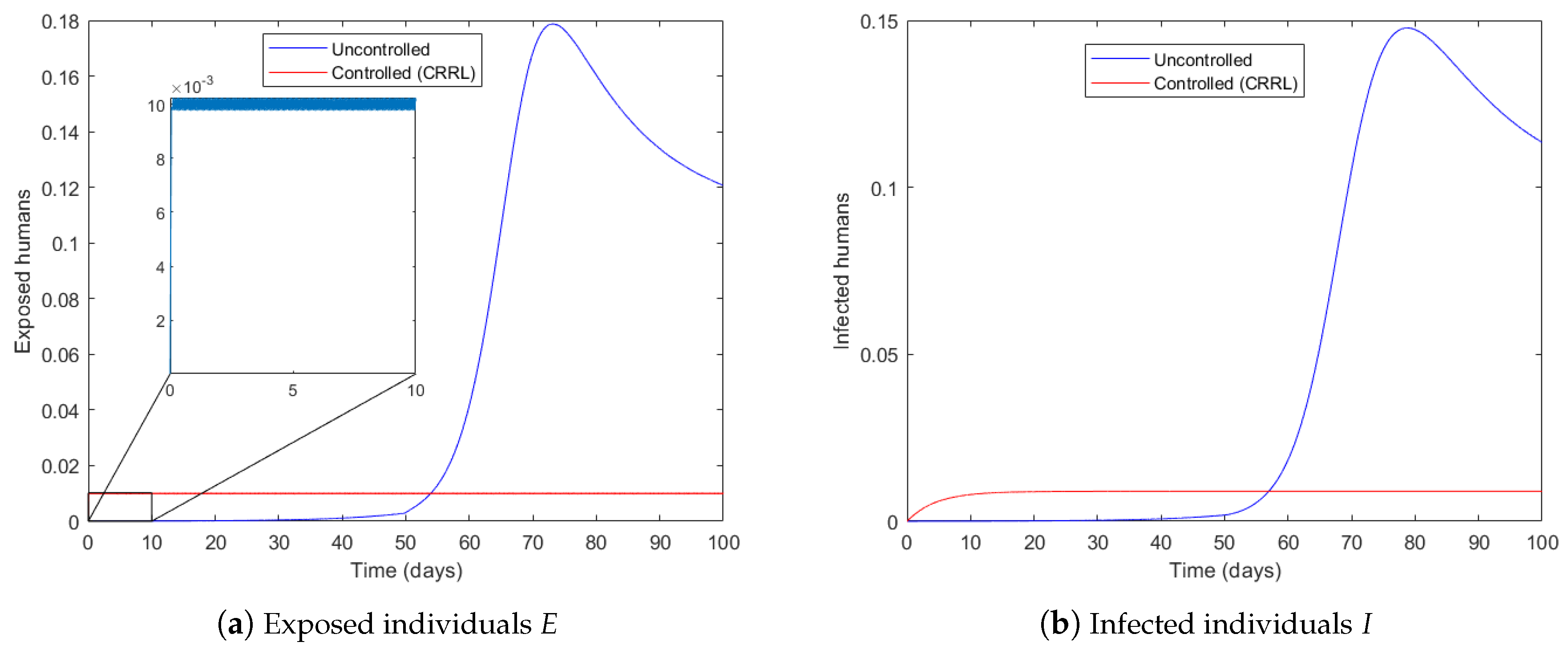
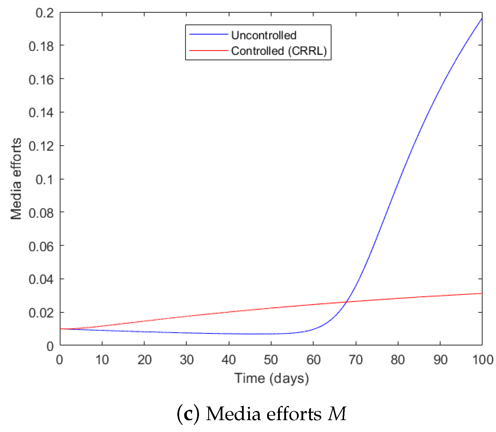
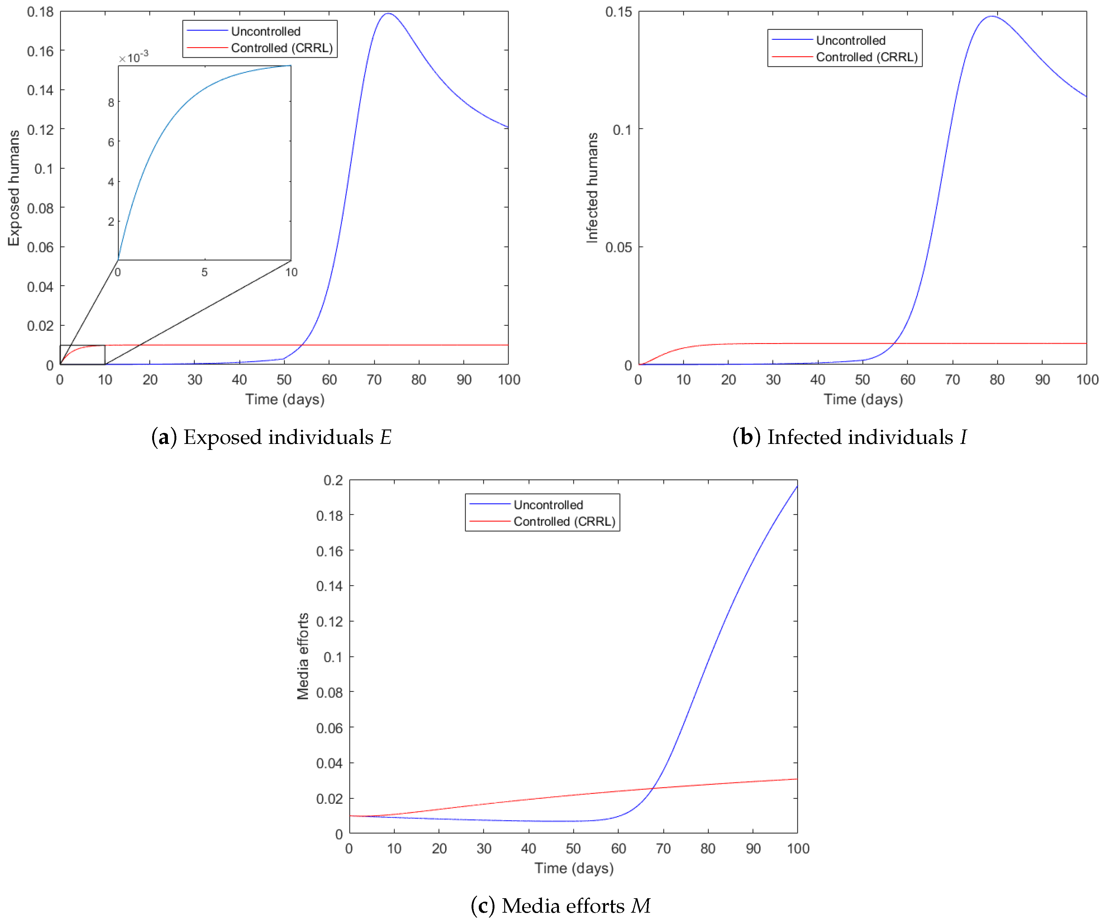
Figure 3 shows the comparison between the controlled and uncontrolled responses for the (CRRL). It is seen from Figure 3a that the exposed individuals’ trajectory E quickly reaches the desired level E d = 0.01 and stays there for the rest of the simulation. Note that the expected chattering effect is also seen here. The fraction of the infected individuals I also reaches about 0.01 at around Day 10 and stay at that point onward. Note that the final value of the infected individuals compartment is also the same as E d . The uncontrolled trajectories for the E and I populations exponentially increase after Day 60, reaching a peak of 0.15 and decays down to about 0.1, as was described in Section 2.4. The media efforts appear to increase somewhat linearly during control, suggesting that governmental interaction control also keeps the rate of expending the media efforts constant. This is in contrast to the uncontrolled system, where the media efforts largely stay at a constant level initially, then increases without bound.
Figure 4 compares the trajectories between the controlled and uncontrolled responses for the power law with m = 1 . Notice that the responses are similar to Figure 3 with respect to the general trend. However the chattering effect seen in Figure 3a is eliminated with application of the power law. In practice, this chattering effect does not affect the actuation process, which in this case is governmental interaction, rather than an electrical motor or a control valve that could be subjected to wear and tear.

4.2. Vaccination Strategy

Having seen the governmental interaction strategy in terms of how it would affect the system, we now turn our attention to the vaccination strategy. The initial condition used is [0.5,0,0,0,0] T . The parameters c 1 , c 2 , and c 3 are chosen as:
c 1 = 0.5 , c 2 = 0.3 , c 3 = 0.1
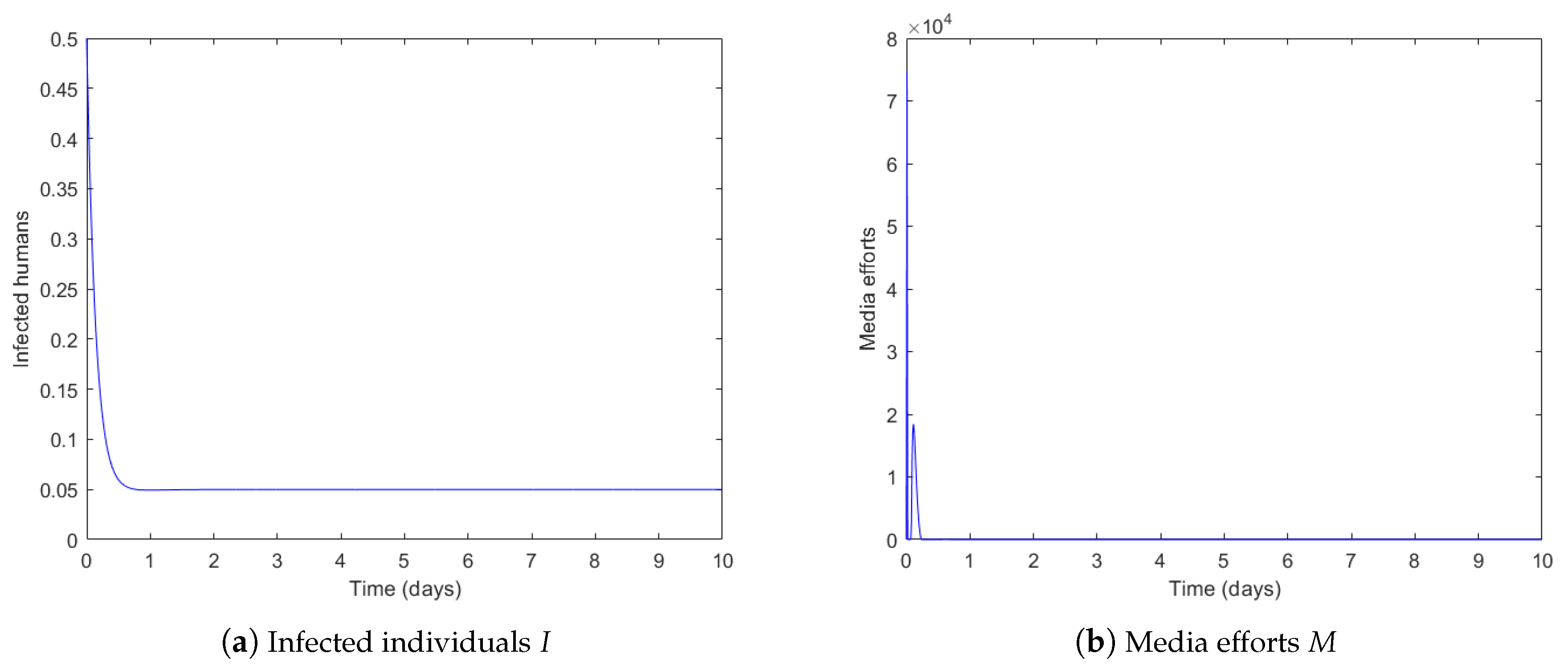
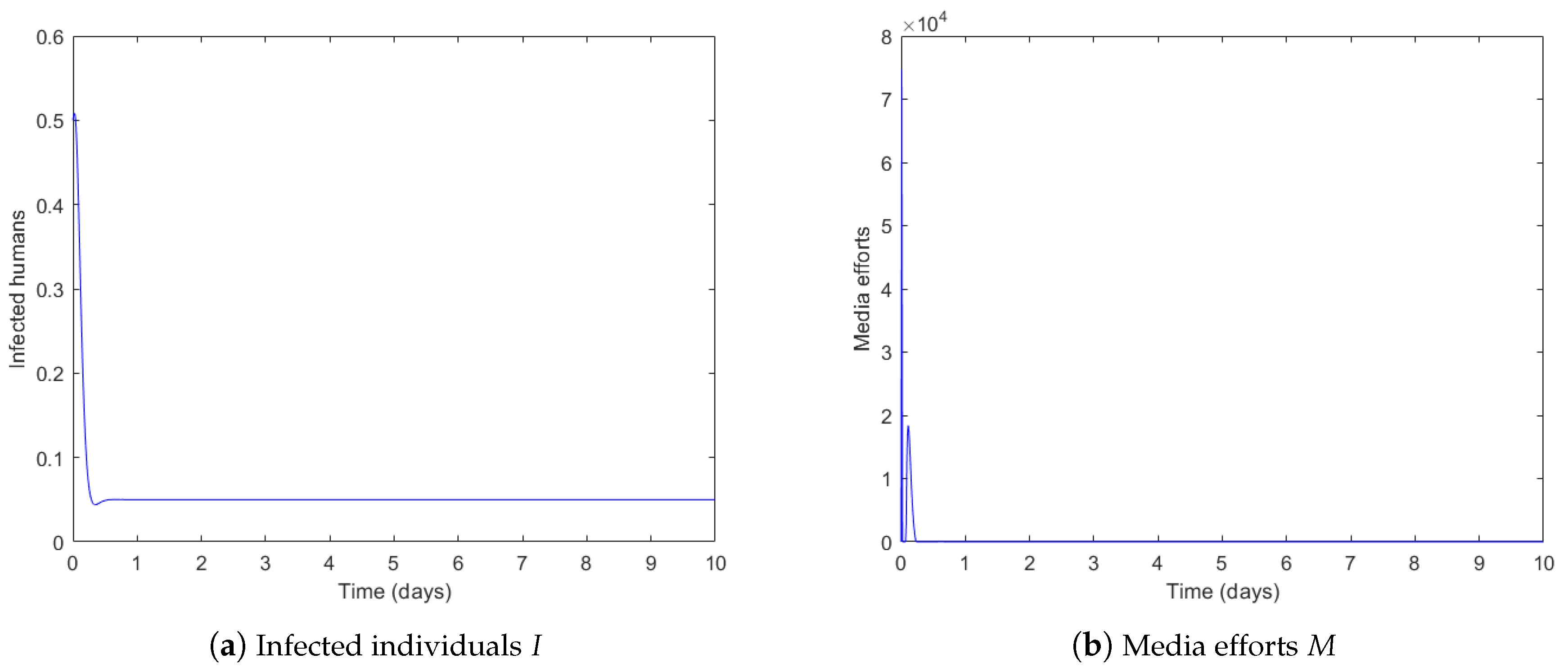
The k 2 parameter is chosen to be k 2 = 2 . Note that only the power reaching law case with m = 1 is shown for ease of implementation and demonstration. The desired infected population level is set at I d = 0.05 . Figure 5 plots the control results for the vaccination strategy. Figure 5a plots the proportion of the infected population I for the vaccination control strategy. It is seen that the infected population quickly reaches the reference level as desired, with no apparent overshooting. Note that no apparent chattering effect is seen due to the use of the power law instead of the CRRL. The media efforts, as depicted in Figure 5b, is quite huge at first, which coincides with the trajectory of the infected individuals. Once the desired value is reached, the media efforts are minimal. This result suggests that enormous media efforts are required to usher the population to receive their vaccination. Once critical vaccination threshold is reached, the efforts required would be minimal. This scenario does not consider the effect of public disinformation as well as vaccine debasements. Studies into the effects of public disinformation is best left for future work.
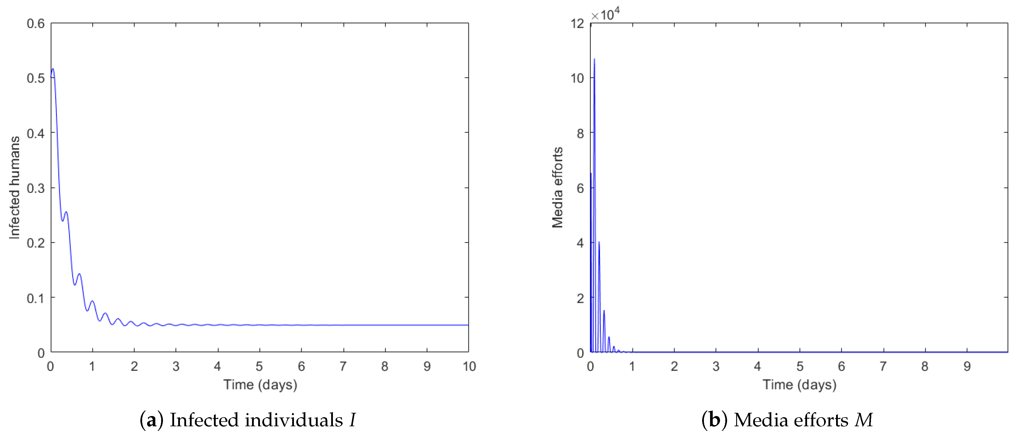
To investigate the effect of the imperfect vaccination, we suppose that the efficacy constant ϵ a is 0.85–0.95. That is, the vaccine is only 88–95% effective, based on recent studies [46,47,48,49]. Figure 6 plots the proportion of the infected population I for the sliding mode vaccination control, with the constant ϵ a assumed to be 0.85. As is seen, the controlled population again quickly reaches the desired value, albeit experiencing a little oscillation on the way. The media efforts M is again quite large initially and diminishes as the controlled population reaches its desired value. Nevertheless, these results also show that the designed controller is largely robust to input changes as well.
To test the robustness of the control algorithm in face of disturbances, let us suppose that a new cluster of individuals at up to twice the sum of the exposed and infected classes are now exposed to the disease. This new cluster of individuals are treated as disturbances. Figure 7 plots the proportion of the infected population I and the media efforts M for the vaccination control in the presence of such a significant disturbance. As is seen, the infected population response exhibits some significant transients as it converges towards the reference. The media efforts signal M is again enormous initially but exponentially decays to zero just before the infected trajectory reaches the desired level. This result validates the robustness of the nonlinear sliding mode control that even though significant disturbances are present, the desired control is still achieved effectively. Note also that these disturbances can also arise from stochastic sources. The use of the sliding mode control would also compensate for these effects as well. As an extension to the stochastic phenomenon, a full stochastic SEIR model has previously been proposed in [15], while the sliding mode control for a Markov jump system was previously explored in [33,34]. It would indeed be of interest to design a sliding mode control for the Markov jump SEIR model.

5. Conclusions

In the face of COVID-19, a terrifying disease, governmental administrations all over the world are actively attempting to combat the deadly disease in their own way, with varying successes. In this work, a simple mathematical model that is based on the basic SEIR framework, whilst incorporating nonlinear incidence, along with governmental interactions and media effects is detailed. The main dynamical properties of the model such as positivity, stability, and sensitivity were investigated first. The proposed control algorithm followed the sliding mode control framework. The main control objective is to simply contain the number of infected individuals at a desired level, so that extreme measures such as lockdowns could be relaxed. Two policies were investigated. The first policy centered on governmental interaction, where the control actively determined an appropriate value of measure based on the intensity of the infection. The second policy centered on inoculation, which necessitated a transformation of the original model into the normal form to allow for the sliding mode controller to be designed. For both control policies, two widely used sliding mode reaching laws were considered: the constant rate reaching law (CRRL) and the power law. Simulation results showed that both control policies were effective in containing the disease, while keeping the rate of media efforts expenses constant. Note that with the age of social media, public disinformation resulting from the spread of rumors is an integral factor determining the success of a vaccination program. Such phenomenon will form the subject of our future work.

Funding

This research received no external funding.

Institutional Review Board Statement

Not applicable.

Informed Consent Statement

Not applicable.

Data Availability Statement

The data is available from the author upon reasonable requests.

Acknowledgments

The author would like to acknowledge the anonymous reviewers for their helpful comments and suggestions.

Conflicts of Interest

The author declares no conflict of interest.

Appendix A. Derivations and Proofs

Appendix A.1

Following the definition of the states introduced in Equation (58), differentiating ξ 1 with respect to time yields:
ξ ˙ 1 = x ˙ 4 = σ x 2 ( μ + μ d + r ) x 4 = ξ 2
The time derivative of ξ 2 is:
ξ ˙ 2 = σ x ˙ 2 ( μ + μ d + r ) x ˙ 4 = ξ 3
To obtain the time derivative of ξ 3 , we first need the definition of x 2 in terms of ξ 1 and ξ 2 . This is simply attained from the solving of the L f h ( x ) equation:
x 2 = ( μ + μ d + r ) ξ 1 + ξ 2 σ
Substituting the result of Equation (A3) for x 2 and solving the ξ 3 equation for x 1 now yields:
x 1 = 1 β 0 σ ξ 1 ( 1 + α ξ 1 2 ) ( ( μ + μ d + r ) ( μ σ ) ξ 1 + ( μ d + r + σ ) ξ 2 + ξ 3 )
The time derivative of ξ 3 , including the definitions of x 1 and x 2 in Equations (A3) and (A4) is:
ξ ˙ 3 = 1 1 + α ξ 1 2 ( ( 2 μ + μ d + r + σ ) ( 1 + α ξ 1 2 ) ( 2 μ ( μ + μ d + r ) ξ 1 + ( μ μ d r ) ξ 2 ξ 3 ) + ξ 2 ( ( μ + μ d + r ) 2 ( 1 + α ξ 1 2 ) + ( 1 α ξ 1 2 ) ( ( μ + μ d + r ) ( μ σ ) ξ 1 + ( μ d + r + σ ) ξ 2 + ξ 3 ) ξ 1 ) + β 0 σ ξ 1 ( μ ( ( μ + μ d + r ) ( μ σ ) ξ 1 + ( μ d + r + σ ) ξ 2 + ξ 3 σ ) + μ ( 1 + α ξ 1 2 ) × ( ( μ + μ d + r ) ( μ σ ) ξ 1 + ( μ d + r + σ ) ξ 2 + ξ 3 ( β 0 σ ξ 1 ) ) + δ 3 z 1 β ( 1 + α ξ 1 2 ) × ( μ + μ d + r ) ( μ σ ) ξ 1 + ( ( μ d + r + σ ) ξ 2 + ξ 3 ) z 2 β 0 σ ξ 1 ( 1 + γ z 2 ) ) + β 0 σ ξ 1 1 + α ξ 1 2 u ( t )
The derivative of z 1 with respect to time is simply:
z ˙ 1 = ( δ 3 + μ ) z 1 + ( β ( 1 + α ξ 1 2 ) ( ( μ + μ d + r ) ( μ σ ) ξ 1 + ( ( μ d + r + σ ) ξ 2 + ξ 3 ) z 2 β 0 σ ξ 1 ( 1 + γ z 2 ) )
Finally, the time derivative of z 2 is:
z ˙ 2 = x ˙ 5 = μ m ξ 1 μ 0 z 2

Appendix A.2

Zeroing the ξ 1 , ξ 2 and ξ 3 terms, the resulting zero dynamics in Equation (59) are written as:
z ˙ ( t ) = A z
where the transition matrix A is:
A = ( δ 3 + μ ) 0 0 μ 0
It is obvious that this matrix has only negative eigenvalues, implying that the solution to the matrix differential equation in Equation (A8) is exp ( A t ) z ( 0 ) , which is exponentially stable for any initial zero state z ( 0 ) = [ z 1 ( 0 ) , z 2 ( 0 ) ] T .

References

  1. GBD 2019 Diseases and Injuries Collaborators. Global burden of 369 diseases and injuries, 1990–2019: A systematic analysis for the Global Burden of Disease Study 2019. Lancet 2020, 396, 1204–1222. [Google Scholar] [CrossRef]
  2. Centers for Disease Control and Prevention. Diseases and Vaccines Included. Available online: www.cdc.gov (accessed on 10 March 2022).
  3. Kermack, W.O.; McKendrick, A.G. A contribution to the mathematical theory of epidemics. Proc. R. Soc. Lond. Ser. A 1927, 115, 700–721. [Google Scholar]
  4. Huang, S.Z. A new SEIR epidemic model with applications to the theory of eradication and control of diseases, and to the calculation of R0. Math. Biosci. 2008, 215, 84–104. [Google Scholar] [CrossRef] [PubMed]
  5. Pongsumpun, P.; Tang, I.M.; Wongvanich, N. Optimal control of the dengue dynamical transmission with vertical transmission. Adv. Diff. Eqn. 2019, 176. [Google Scholar] [CrossRef] [Green Version]
  6. Lamwong, J.; Wongvanich, N.; Tang, I.M.; Changpuek, K.; Pongsumpun, P. Global Stability of the Transmission of Hand-Foot-Mouth Disease According to the Age Structure of the Population. Curr. Appl. Sci. Tech. 2021, 2, 351–369. [Google Scholar]
  7. Xiao, D.; Ruan, S. Global analysis of an epidemic model with nonmonotone incidence rate. Math. Biosci. 2007, 208, 419–429. [Google Scholar]
  8. Upadhyay, R.K.; Pal, A.K.; Kumari, S.; Roy, P. Dynamics of an SEIR epidemic model with nonlinear incidence and treatment rates. Nonlinear Dyn. 2019, 96, 2351–2368. [Google Scholar] [CrossRef]
  9. Gao, D.P.; Huang, N.J. Threshold dynamics of an SEIR epidemic model with a nonlinear incidence rate and a discontinuous treatment function. RACSAM 2020, 114, 5. [Google Scholar] [CrossRef]
  10. Chen, L.; Wei, F. Study on a susceptible–exposed–infected–recovered model with nonlinear incidence rate. Adv. Differ. Equ. 2020, 206. [Google Scholar] [CrossRef]
  11. Casagradi, R.; Bolzoni, L.; Levin, S.A.; Andreasen, V. The SIRC model and influenza A. Math. Biosci. 2006, 200, 152169. [Google Scholar]
  12. Morrison, R.E.; Cunha, A., Jr. Embedded model discrepancy: A case study of Zika modeling. Chaos 2020, 30, 051103. [Google Scholar] [CrossRef] [PubMed]
  13. Lipsitch, M.; Cohen, T.; Cooper, B.; Robins, J.M.; Ma, S.; James, L.; Gopalakrishna, G.; Chew, S.K.; Tan, C.C.; Samore, M.H.; et al. Transmission dynamics and control of severe acute respiratory syndrome. Science 2003, 300, 19661970. [Google Scholar] [CrossRef] [PubMed] [Green Version]
  14. Ingemar, N. Stochastic models of some endemic infections. Math. Biosci. 2002, 179, 1–19. [Google Scholar]
  15. Guy, R.; Laredo, C.; Vergu, E. Approximation of epidemic models by diffusion processes and their statistical inference. J. Math. Biol. 2015, 70, 621–646. [Google Scholar] [CrossRef] [PubMed]
  16. Misra, A.K.; Sharma, A.; Shukla, J.B. Modeling and analysis of effects of awareness programs by media on the spread of infectious diseases. Math. Comput. Model 2011, 53, 1221–1228. [Google Scholar] [CrossRef]
  17. Tchuenche, J.M.; Dube, N.; Bhunu, C.P.; Smith, R.J.; Bauch, C.T. The impact of media coverage on the transmission dynamics of human influenza. BMC Publ. Health 2011, 11 (Suppl. S1), S5. [Google Scholar] [CrossRef] [Green Version]
  18. Dubey, B.; Dubey, P.; Dubey, U. Role of media and treatment on SIR model. Nonl. Anal. Model. Control. 2015, 21, 185–200. [Google Scholar] [CrossRef]
  19. Ding, Y.; Jiao, J.; Zhang, Q.; Zhang, Y.; Ren, X. Stationary Distribution and Extinction in a Stochastic SIQR Epidemic Model Incorporating Media Coverage and Markovian Switching. Symmetry 2021, 13, 1122. [Google Scholar] [CrossRef]
  20. Rodrigues, H.S.; Monteiro, M.T.; Torres, D.F.M. Dynamics of Dengue epidemics when using optimal control. Math. Comput. Model. 2010, 52, 1667–1673. [Google Scholar] [CrossRef] [Green Version]
  21. Imran, M.; Usman, M.; Malik, T.; Ansari, A.R. Mathematical analysis of the role of hospitalization/isolation in controlling the spread of Zika fever. Virus Res. 2018, 255, 95–104. [Google Scholar] [CrossRef]
  22. Momoh, A.A.; Fuegenschuh, A. Optimal control of intervention strategies and cost effectiveness analysis for a Zika virus model. Oper. Res. Health. Care 2018, 18, 99–111. [Google Scholar] [CrossRef]
  23. Wongvanich, N.; Tang, I.-M.; Dubois, M.-A.; Pongsumpun, P. Mathematical Modeling and Optimal Control of the Hand Foot Mouth Disease Affected by Regional Residency in Thailand. Mathematics 2021, 9, 2863. [Google Scholar] [CrossRef]
  24. Agarwal, R.P.; Mofarreh, F.; Shah, R.; Luangboon, W.; Nonlaopon, K. An Analytical Technique, Based on Natural Transform to Solve Fractional-Order Parabolic Equations. Entropy 2021, 23, 1086. [Google Scholar] [CrossRef] [PubMed]
  25. Levant, A. Sliding order and sliding accuracy in sliding mode control. Int. J. Control. 1993, 58, 1247–1263. [Google Scholar] [CrossRef]
  26. Shtessel, Y.; Edwards, C.; Fridman, L.; Levant, A. Sliding Mode Control and Observation. In Control Engineering; Springer Science+Business Media: New York, NY, USA, 2014; Volume 10. [Google Scholar]
  27. Zhang, B.; Yang, X.; Zhao, D.; Spurgeon, S.K.; Yan, X. Sliding Mode Control for Nonlinear Manipulator Systems. IFAC-Pap. Online 2017, 50, 5127–5132. [Google Scholar] [CrossRef]
  28. Fang, Y.; Fu, W.; An, C.; Yuan, Z.; Fei, J. Modelling, Simulation and Dynamic Sliding Mode Control of a MEMS Gyroscope. Micromachines 2021, 12, 190. [Google Scholar] [CrossRef]
  29. Zhou, K.; Yuan, C.; Sun, D.; Jin, N.; Wu, X. Parameter adaptive terminal sliding mode control for full-bridge DC-DC converter. PLoS ONE 2021, 16, e0247228. [Google Scholar] [CrossRef]
  30. Zheng, B.; Wu, Y.; Li, H.; Chen, Z. Adaptive Sliding Mode Attitude Control of Quadrotor UAVs Based on the Delta Operator Framework. Symmetry 2022, 14, 498. [Google Scholar] [CrossRef]
  31. Shi, P.; Xia, Y.; Liu, G.P.; Rees, D. On designing of sliding-mode control for stochastic jump systems. IEEE Trans. Autom. Control. 2006, 51, 97–103. [Google Scholar] [CrossRef]
  32. Niu, Y.; Ho, D.W.C.; Wang, X. Sliding mode control for Itô stochastic systems with Markovian switching. Automatica 2007, 43, 1784–1790. [Google Scholar] [CrossRef]
  33. Zhang, H.; Shen, M. Sliding mode H-∞ control of time-varying delay Markov jump with quantized output. Optim. Control. Appl. Methods 2019, 40, 226–240. [Google Scholar] [CrossRef]
  34. Shen, M.; Zhang, H.; Park, J.H. Observer-based quantized sliding mode H-∞ control of Markov jump systems. Nonlinear Dyn. 2018, 92, 415–427. [Google Scholar] [CrossRef]
  35. Khalili Amirabadi, R.; Heydari, A.; Zarrabi, M. Analysis and control of SEIR epedemic model via sliding mode control. Adv. Model. Optim. 2016, 18, 153–162. [Google Scholar]
  36. Sharifi, M.; Moradi, H. Nonlinear robust adaptive sliding mode control of influenza epidemic in the presence of uncertainty. J. Process Control 2017, 56, 48–57. [Google Scholar] [CrossRef]
  37. van den Driessche, P.; Watmough, J. Reproduction number and subthreshold endemic equilibria for compartment models of disease transmission. Math. Biosci. 2002, 180, 29–48. [Google Scholar] [CrossRef]
  38. Rohith, G.; Devika, K.B. Dynamics and control of COVID-19 pandemic with nonlinear incidence rates. Nonlinear Dyn. 2020, 101, 2013–2026. [Google Scholar] [CrossRef]
  39. Chitnis, N.; Hyman, J.M.; Cushing, J.M. Determining important parameters in the spread of malaria through the sensitivity analysis of a mathematical model. Bullet. Math. Biol. 2008, 70, 1272–1296. [Google Scholar] [CrossRef]
  40. Silva, C.J.; Torres, D.F.M. Optimal control for a tuberculosis model with reinfection and post-exposure interventions. Math. Biosci. 2013, 244, 154–164. [Google Scholar] [CrossRef] [Green Version]
  41. Gao, W.; Hung, J.C. Variable structure control of nonlinear systems: A new approach. IEEE Trans. Ind. Electron. 1993, 40, 45–55. [Google Scholar]
  42. Spooner, J.T.; Maggione, M.; Ordonez, R.; Passino, K.M. Stable Adaptive Control and Estimation for Nonlinear Systems: Neural and Fuzzy Approximator Techniques, ser. In Adaptive and Cognitive Dynamic Systems: Signal Processing, Learning, Communications and Control; Wiley: New York, NY, USA, 2002; pp. 141–153. [Google Scholar]
  43. Hangos, K.; Bokor, J.; Szederkenyi, G. Analysis and Control of Nonlinear Process Systems, ser. Advanced Textbooks in Control and Signal Processing; Springer: London, UK, 2006. [Google Scholar]
  44. Brockett, R.W. Nonlinear systems and differential geometry. Proc. IEEE 1976, 64, 61–72. [Google Scholar] [CrossRef]
  45. Zabczyk, J. Mathematical Control Theory: An Introduction, ser. Modern Birkhauser Classics; Birkhauser: Boston, MA, USA, 2009. [Google Scholar]
  46. Ledlord, H. Six months of COVID vaccines: What 1.7 billion doses have taught scientists. Nature 2021, 594, 164–167. [Google Scholar] [CrossRef] [PubMed]
  47. Hass, E.J.; Angulo, F.J.; McLaughlin, J.M.; Anis, E.; Singer, S.R.; Khan, F.; Brooks, N.; Smaja, M.; Mircus, G.; Pan, K.; et al. Impact and effectiveness of mRNA BNT162b2 vaccine against SARS-CoV-2 infections and COVID-19 cases, hospitalisations, and deaths following a nationwide vaccination campaign in Israel: An observational study using national surveillance data. Lancet 2021, 397, 1819–1829. [Google Scholar] [CrossRef]
  48. Frenck, R.W.; Klein, N.P.; Kitchin, N.; Gurtman, A.; Absalon, J.; Lockhart, S.; Perez, J.L.; Walter, E.B.; Senders, S.; Bailey, R.; et al. Safety, Immunogenicity, and Efficacy of the BNT162b2 COVID-19 Vaccine in Adolescents. N. Engl. J. Med. 2021, 385, 239–250. [Google Scholar] [CrossRef] [PubMed]
  49. Bernal, J.L.; Andrews, N.; Gower, C.; Robertson, C.; Stowe, J.; Tessier, E.; Simmons, R.; Cottrell, S.; Roberts, R.; O’Doherty, M.; et al. Effectiveness of the Pfizer-BioNTech and Oxford-AstraZeneca vaccines on COVID-19 related symptoms, hospital admissions, and mortality in older adults in England: Test negative case-control study. Br. Med. J. 2021, 373, n1088. [Google Scholar] [CrossRef] [PubMed]
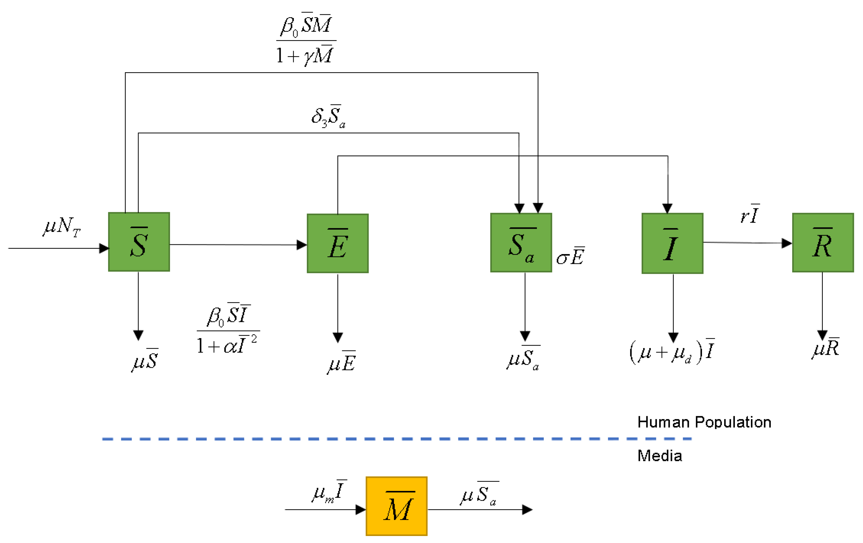
Figure 1. Schematics of the formulated model.
Symmetry 14 01010 g001
Figure 2. Numerical simulation for the open loop system given in Equation (5) with the parameters shown in Table 1.
Symmetry 14 01010 g002
Figure 3. Numerical simulation for the constant rate reaching law (CRRL) sliding mode control for the governmental interaction policy against the uncontrolled system.
Symmetry 14 01010 g003aSymmetry 14 01010 g003b
Figure 4. Numerical simulation for the power reaching law sliding mode control for the governmental interaction policy with m = 1 against the uncontrolled system.
Symmetry 14 01010 g004
Figure 5. The infected population I ( t ) and required media efforts M for the vaccination control strategy.
Symmetry 14 01010 g005
Figure 6. The infected population I ( t ) and required medis efforts M ( t ) for the vaccination control strategy under the assumption of imperfect vaccination with efficacy constant ϵ a = 0.85.
Symmetry 14 01010 g006
Figure 7. The infected population I ( t ) and associated media efforts M for the vaccination control strategy in the presence of disturbances to the system.
Symmetry 14 01010 g007
Table 1. Parameters used in the numerical simulation of the model.
ParameterValues
Birth/death rate, μ 0.08
Contact rate, β 0 0.76
Rate of transfer between the aware susceptible individuals back to susceptibles, δ 3 0.18
Governmental effort, α 10
Media inhibition parameter, γ 20
Rate of transfer between the exposed and infected classes, σ 0.20
Disease recovery rate, r1/7
Disease induced mortality rate, μ d 0.02
Implementation rate of the awareness program, μ m 0.05
Removal rate of the awareness program, μ 0 0.02
Table 2. Forward sensitivity parameter of R 0 with respect to the parameters of Table 1.
ParameterForward Sensitivity Ψ p R 0
μ −0.6151
β 0 1
δ 3 0
α 0
γ 0
σ 0.2857
r−0.5882
μ d −0.082
μ m 0
μ 0 0
Publisher’s Note: MDPI stays neutral with regard to jurisdictional claims in published maps and institutional affiliations.