Algebraic Analysis of Zero-Hopf Bifurcation in a Chua System

Abstract

This article first studies the stability conditions of a Chua system depending on six parameters. After, using the averaging method, as well as the methods of the Gröbner basis and real solution classification, we provide sufficient conditions for the existence of three limit cycles bifurcating from a zero-Hopf equilibrium of the Chua system. As we know, this last phenomena is first found. Some examples are presented to verify the established results.

1. Introduction and Main Results

The Chua system is a simple electronic circuit that exhibits classic chaotic behavior. It was presented in 1986 by Chua, Komuro and Matsumoto [1] and exhibits a rich range of dynamical behavior. Since then, the research on dynamical behaviors of Chua’s system and its generalizations has attracted the extensive interest of scholars; see [2,3,4] for instance. In particular, the authors in [5] found a coexistence limit cycle and symmetric hidden attractors in the Chua system. It was shown in [6] that a modified Chua system can display complex dynamics behaviors of symmetric and asymmetric coexisting attractors. In this paper, we study the following Chua system described by the differential equations

$$\begin{array}{cc}\hfill \dot{x}& =a(z-bx-{\alpha }_2{x}^2-{\alpha }_1{x}^3),\hfill \\ \hfill \dot{y}& =-z,\hfill \\ \hfill \dot{z}& =-{\beta }_{1}x+y+{\beta }_{2}z,\hfill \end{array}$$

(1)

where a, b, ${\alpha }_1$, ${\alpha }_2$, ${\beta }_1$ and ${\beta }_2$ are real parameters.

A few dynamics results for the Chua system are summarized as follows. The existence of local and global analytic first integrals in the Chua system was investigated in [7]. In [8], the authors obtained an analytical expression of the slow manifold equation of the Chua system by using techniques of differential geometry. The dynamics at infinity of system (1) was studied in [9] for the particular case where ${\beta }_1$ and ${\beta }_2$ are both one. Some aspects about the Hopf bifurcation can be found in [10,11].

The goal of this paper is to study how many limit cycles can bifurcate from a zero-Hopf equilibrium of the Chua system (1) by using the second averaging method. We recall that a zero-Hopf equilibrium of a 3D differential system is an isolated equilibrium point $p_0$ such that the Jacobian matrix of the system at $p_0$ has a zero and a pair of purely imaginary eigenvalues. There are many studies of zero-Hopf bifurcations in 3D differential systems; see [12,13,14,15,16,17] and the references therein. We remark that some results on the zero-Hopf bifurcation of system (1) were already obtained by Euzébio and Llibre in [18]. Our objective here is to further study analytically such a bifurcation using the averaging method together with the local stability of the system. Unlike the usual analysis of zero-Hopf bifurcation, by means of symbolic computation, we would like to compute a partition of the parametric space of the involved parameters such that, inside every open cell of the partition, the system can have the maximum number of limit cycles that bifurcate from a zero-Hopf equilibrium.

On the number of equilibria of the Chua system, we recall from [18] that system (1) can have three equilibria, including the origin and the two equilibria

$$\begin{array}{c}\hfill p_{\pm }=\left(\frac{-{\alpha }_2\pm \sqrt{{\alpha }_2^2-4{\alpha }_{1}b}}{2{\alpha }_1},-\frac{{\alpha }_2{\beta }_1}{2{\alpha }_1}\pm \frac{{\beta }_1\sqrt{{\alpha }_2^2-4{\alpha }_{1}b}}{2{\alpha }_1},0\right)\end{array}$$

(2)

if ${\alpha }_2^2-4{\alpha }_{1}b>0$ and ${\alpha }_1\ne 0$, and has only two equilibria, including the origin and the equilibrium

$$p=\left(-\frac{{\alpha }_2}{2{\alpha }_1},-\frac{{\alpha }_2{\beta }_1}{2{\alpha }_1},0\right)$$

when ${\alpha }_2^2-4{\alpha }_{1}b=0$ and ${\alpha }_1{\alpha }_2\ne 0$. Otherwise, the origin is the unique equilibrium of the system.

Motivated by the above results, our first goal of this paper is to study conditions on the parameters under which the Chua system (1) has a prescribed number of stable equilibrium points. Our result on this question is the following, and its proof can be found in Section 3.

Proposition 1.

The Chua system (1) cannot have three stable equilibrium points; it has two stable equilibrium points if the following condition

$$\begin{array}{c}\hfill {\mathcal{C}}_1=[T_1<0,T_2\le 0,0\le T_3,T_4<0]\wedge {\mathcal{C}}_0\end{array}$$

(3)

holds; and it has one stable equilibrium point if one of the following three conditions

$$\begin{array}{cc}\hfill {\mathcal{C}}_2& =[T_1<0,T_3\le 0]\wedge {\mathcal{C}}_0,\hfill \\ \hfill {\mathcal{C}}_3& =[T_1<0,0\le T_3,0<T_4]\wedge {\mathcal{C}}_0,\hfill \\ \hfill {\mathcal{C}}_4& =[0<T_1,T_2\le 0,0\le T_3,T_4<0]\wedge {\mathcal{C}}_0\hfill \end{array}$$

(4)

holds. Here, ${\mathcal{C}}_0=[{\beta }_2=1,ab-1>0,{\alpha }_1>0]$, and

$$\begin{array}{cc}\hfill T_1=& a^2{b}^2-a^{2}b{\beta }_1-ab+a{\beta }_1+1,\hfill \\ \hfill T_2=& 4a^2{b}^2{\alpha }_1^2+2a^{2}b{\alpha }_1^2{\beta }_1-5a^{2}b{\alpha }_1{\alpha }_2^2-a^2{\alpha }_1{\alpha }_2^2{\beta }_1+a^2{\alpha }_2^4+2ab{\alpha }_1^2\hfill \\ \hfill & +a{\alpha }_1^2{\beta }_1-a{\alpha }_1{\alpha }_2^2+{\alpha }_1^2,\hfill \\ \hfill T_3=& 16a^3{b}^3{\alpha }_1^3+8a^3{b}^2{\alpha }_1^3{\beta }_1-24a^3{b}^2{\alpha }_1^2{\alpha }_2^2-6a^{3}b{\alpha }_1^2{\alpha }_2^2{\beta }_1+9a^{3}b{\alpha }_1{\alpha }_2^4+a^3{\alpha }_1{\alpha }_2^4{\beta }_1\hfill \\ \hfill & -a^3{\alpha }_2^6+16a^2{b}^2{\alpha }_1^3+8a^{2}b{\alpha }_1^3{\beta }_1-12a^{2}b{\alpha }_1^2{\alpha }_2^2-2a^2{\alpha }_1^2{\alpha }_2^2{\beta }_1+2a^2{\alpha }_1{\alpha }_2^4+8ab{\alpha }_1^3\hfill \\ \hfill & +2a{\alpha }_1^3{\beta }_1-2a{\alpha }_1^2{\alpha }_2^2+2{\alpha }_1^3,\hfill \\ \hfill T_4=& 16a^4{b}^4{\alpha }_1^2+16a^4{b}^3{\alpha }_1^2{\beta }_1-8a^4{b}^3{\alpha }_1{\alpha }_2^2+4a^4{b}^2{\alpha }_1^2{\beta }_1^2-8a^4{b}^2{\alpha }_1{\alpha }_2^2{\beta }_1+a^4{b}^2{\alpha }_2^4\hfill \\ \hfill & -a^{4}b{\alpha }_1{\alpha }_2^2{\beta }_1^2+a^{4}b{\alpha }_2^4{\beta }_1+16a^3{b}^3{\alpha }_1^2+16a^3{b}^2{\alpha }_1^2{\beta }_1-8a^3{b}^2{\alpha }_1{\alpha }_2^2+4a^{3}b{\alpha }_1^2{\beta }_1^2\hfill \\ \hfill & -8a^{3}b{\alpha }_1{\alpha }_2^2{\beta }_1+a^{3}b{\alpha }_2^4-a^3{\alpha }_1{\alpha }_2^2{\beta }_1^2+a^3{\alpha }_2^4{\beta }_1+12a^2{b}^2{\alpha }_1^2+8a^{2}b{\alpha }_1^2{\beta }_1-7a^{2}b{\alpha }_1{\alpha }_2^2\hfill \\ \hfill & +a^2{\alpha }_1^2{\beta }_1^2-2a^2{\alpha }_1{\alpha }_2^2{\beta }_1+a^2{\alpha }_2^4+4ab{\alpha }_1^2+2a{\alpha }_1^2{\beta }_1-a{\alpha }_1{\alpha }_2^2+{\alpha }_1^2.\hfill \end{array}$$

(5)

Remark 1.

We remark that the condition ${\mathcal{C}}_0$ is used to facilitate the computation of the resulting semi-algebraic system (see Section 3) since the algebraic analysis usually involves heavy computation; see [19,20].

Example 1.

Let

$$\begin{array}{c}\hfill \left(a,b,{\alpha }_1,{\alpha }_2,{\beta }_1,{\beta }_2\right)=\left(1,2,1,4,4,1\right)\in {\mathcal{C}}_2.\end{array}$$

Then the Chua system (1) becomes

$$\begin{array}{cc}\hfill & \dot{x}=z-2x-4x^2-x^3,\hfill \\ \hfill & \dot{y}=-z,\hfill \\ \hfill & \dot{z}=-4x+y+z.\hfill \end{array}$$

(6)

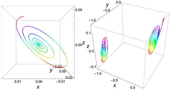
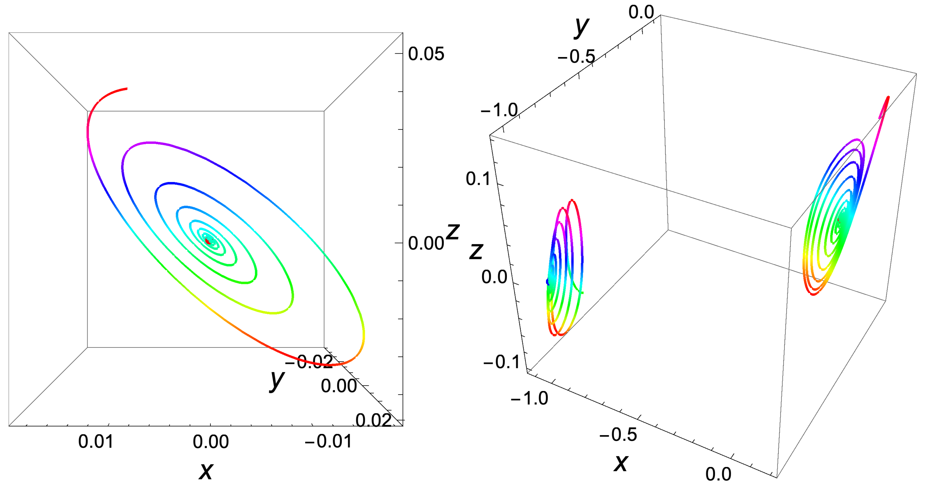
Its three equilibria are: $p=(0,0,0)$, $p_{\pm }=(-2\pm \sqrt{2},4(-2\pm \sqrt{2}),0)$. System (6) has only one stable equilibrium point p; see Figure 1 (left).

Figure 1. Numerical simulations of local asymptotically stability of the Chua system. (letf) Stability of system (6). (right) Stability of system (7).

Example 2.

Let

$$\begin{array}{c}\hfill \left(a,b,{\alpha }_1,{\alpha }_2,{\beta }_1,{\beta }_2\right)=\left(4,\frac{1}{2},1,\frac{3}{2},1,1\right)\in {\mathcal{C}}_1.\end{array}$$

Then the Chua system (1) becomes

$$\begin{array}{cc}\hfill & \dot{x}=4z-2x-6x^2-4x^3,\hfill \\ \hfill & \dot{y}=-z,\hfill \\ \hfill & \dot{z}=-x+y+z.\hfill \end{array}$$

(7)

It has three equilibria: $p=(0,0,0)$, $p_{+}=(-\frac{1}{2},-\frac{1}{2},0)$ and $p_{-}=(-1,-1,0)$. Two of them (p and $p_{-}$) are stable; see Figure 1 (right).

It is shown by Euzébio and Llibre in [18] that there are three 4-parameter families of Chua systems exhibiting a zero-Hopf equilibrium (see Proposition 1 in [18]). In particular, the origin is a zero-Hopf equilibrium when $b={\beta }_2=0$ and $a{\beta }_1+1={\omega }^2>0$. In this case, the linear part of the Chua system at the origin has the eigenvalues 0 and $\pm i\omega$ with $\omega \ne 0$. Euzébio and Llibre proved that for the first order averaging, 1 limit cycle can bifurcate from the origin and up to the second order averaging, 1, 2 or 3 limit cycles can bifurcate simultaneously from the other two families. The goal of this paper is to obtain further results on the bifurcation limit cycles from the origin of the Chua system (1). The main techniques are based on the second order averaging method and some algebraic methods, such as the Gröbner basis [21] and real root classifications [22]. The techniques used here for studying the zero-Hopf bifurcation can be applied to other high dimensional polynomial differential systems.

We consider the vector $(a,b,{\alpha }_1,{\alpha }_2,{\beta }_1,{\beta }_2)$ given by

$$\begin{array}{cc}\hfill a& ={\gamma }_0+\epsilon {\alpha }_{1,0}+{\epsilon }^2{\alpha }_{2,0},\hspace{1em}b=\epsilon {\beta }_{1,0}+{\epsilon }^2{\beta }_{2,0},\hfill \\ \hfill {\alpha }_1& ={\gamma }_1+\epsilon {\alpha }_{1,1}+{\epsilon }^2{\alpha }_{2,1},\hspace{1em}{\alpha }_2={\gamma }_2+\epsilon {\alpha }_{1,2}+{\epsilon }^2{\alpha }_{2,2},\hfill \\ \hfill {\beta }_1& =\frac{{\omega }^2-1}{a}+\epsilon {\beta }_{1,1}+{\epsilon }^2{\beta }_{2,1},\hspace{1em}{\beta }_2=\epsilon {\beta }_{1,2}+{\epsilon }^2{\beta }_{2,2},\hfill \end{array}$$

(8)

where $\epsilon \ne 0$ is a sufficiently small parameter, the constants ${\gamma }_i$, ${\alpha }_{i,j}$ and ${\beta }_{i,j}$ are all real parameters. The main result on the number of limit cycles of the Chua system is stated as follows.

Theorem 2.

The following statements are for $\epsilon \ne 0$ that is sufficiently small and the vector given by (8).

(i)

System (1) has, up to the first order averaging, at most 1 limit cycle bifurcates from the origin, and this number can be reached if one of the following two conditions holds:

$$\begin{array}{c}\hfill {\mathcal{C}}_5=[R_1<0,R_2<0]\wedge \overline{\mathcal{C}},{\mathcal{C}}_6=[0<R_1,0<R_2]\wedge \overline{\mathcal{C}},\end{array}$$

(9)

where

$$\begin{array}{cc}\hfill R_1& =({\omega }^2-1){\beta }_{1,0}{\gamma }_0+{\omega }^2{\beta }_{1,2},\hfill \\ \hfill R_2& =({\omega }^2-1){\beta }_{1,0}{\gamma }_0-{\omega }^2{\beta }_{1,2},\hfill \\ \hfill \overline{\mathcal{C}}& =[\omega \notin \{-1,0,1\},{\gamma }_0\ne 0,{\gamma }_2\ne 0].\hfill \end{array}$$

(ii)

System (1) has, up to the second order averaging, at most 3 limit cycles that bifurcate from the origin, and this number can be reached if the following condition holds:

$$\begin{array}{cc}\hfill {\mathcal{C}}_7& =[{\overline{R}}_1<0,{\overline{R}}_2<0,{\overline{R}}_3\le 0,0<{\overline{R}}_4]\wedge {\mathcal{C}}^{*},\hfill \end{array}$$

(10)

where ${\mathcal{C}}^{*}=[\omega ={\beta }_{2,0}={\alpha }_{1,2}=2,{\gamma }_0>0]$, and the explicit expressions of ${\overline{R}}_i$ for $i=1,\dots ,4$ are as follows:

$$\begin{array}{cc}\hfill {\overline{R}}_1& =2{\beta }_{2,2}-3{\gamma }_0,\hfill \\ \hfill {\overline{R}}_2& =2{\beta }_{2,2}^2{\gamma }_1+12{\beta }_{2,2}{\gamma }_0{\gamma }_1+18{\gamma }_0^2{\gamma }_1-6{\beta }_{2,2}{\gamma }_0-9{\gamma }_0^2,\hfill \\ \hfill {\overline{R}}_3& =16{\beta }_{2,2}^3{\gamma }_1^3-36{\beta }_{2,2}^2{\gamma }_0{\gamma }_1^3-198{\beta }_{2,2}{\gamma }_0^2{\gamma }_1^3+162{\gamma }_0^3{\gamma }_1^3+24{\beta }_{2,2}^2{\gamma }_0{\gamma }_1^2+264{\beta }_{2,2}{\gamma }_0^2{\gamma }_1^2\hfill \\ \hfill & +81{\gamma }_0^3{\gamma }_1^2-88{\beta }_{2,2}{\gamma }_0^2{\gamma }_1-144{\gamma }_0^3{\gamma }_1+32{\gamma }_0^3,\hfill \\ \hfill {\overline{R}}_4& =128{\beta }_{2,2}^3{\gamma }_1^3-288{\beta }_{2,2}^2{\gamma }_0{\gamma }_1^3+216{\beta }_{2,2}{\gamma }_0^2{\gamma }_1^3-54{\gamma }_0^3{\gamma }_1^3+192{\beta }_{2,2}^2{\gamma }_0{\gamma }_1^2-288{\beta }_{2,2}{\gamma }_0^2{\gamma }_1^2\hfill \\ \hfill & -297{\gamma }_0^3{\gamma }_1^2+96{\beta }_{2,2}{\gamma }_0^2{\gamma }_1+288{\gamma }_0^3{\gamma }_1-64{\gamma }_0^3.\hfill \end{array}$$

Theorem 2 shows that the Chua system (1) can have exactly 3 limit cycles bifurcating from the origin if the condition in (10) holds. In the following, we provide a concrete example of the Chua system (1) to verify this established result.

Corollary 3.

Consider the special family of the Chua system

$$\begin{array}{cc}\hfill \dot{x}& =2z-4{\epsilon }^{2}x-4\epsilon x^2+4x^3,\hfill \\ \hfill \dot{y}& =-z,\hfill \\ \hfill \dot{z}& =-\frac{3}{2}x+y-{\epsilon }^{2}z,\hfill \end{array}$$

(11)

where $\epsilon \ne 0$ is a sufficiently small parameter. Then system (11), up to the second order averaging, has exactly 3 limit cycles $(x_i(t,\epsilon ),y_i(t,\epsilon ),z_i(t,\epsilon ))$ bifurcating from the origin, namely,

$$\begin{array}{cc}\hfill x_i(t,\epsilon )& =\epsilon \left(\frac{1}{2}{W}_i+R_{i}sin\left(2t\right)\right)+\mathcal{O}\left({\epsilon }^3\right),\hfill \\ \hfill y_i(t,\epsilon )& =\epsilon \left(\frac{3}{4}{W}_i-\frac{1}{2}{R}_{i}sin\left(2t\right)\right)+\mathcal{O}\left({\epsilon }^3\right),\hfill \\ \hfill z_i(t,\epsilon )& =\epsilon R_{i}cos\left(2t\right)+\mathcal{O}\left({\epsilon }^3\right),i=1,2,3,\hfill \end{array}$$

where $(R_i,W_i)$ are solutions of a semi-algebraic system; see Section 5. Moreover, two of the three limit cycles are semistable, and the other one is unstable.

The rest of this paper is organized as follows. In Section 2, we recall the second order averaging method that we shall use for proving the main results. Section 3 is devoted to prove Proposition 1. The proofs of Theorem 2 and Corollary 3 are given in Section 4 and Section 5, respectively. The paper is concluded with a few remarks.

2. Preliminary Results

The averaging method for studying periodic orbits of nonlinear differential systems up to the second order in $\epsilon$ was developed in [23]. Recently, this theory was extended to an arbitrary order in $\epsilon$ for arbitrary dimensional differential systems, see [24]. More discussions on the averaging method, including some applications, can be found in [25,26].

We deal with differential systems in the form

$$\begin{array}{c}\hfill \dot{\mathbf{x}}=\epsilon F_1(t,\mathbf{x})+{\epsilon }^2{F}_2(t,\mathbf{x})+{\epsilon }^{3}R(t,\mathbf{x},\epsilon ),\end{array}$$

(12)

where $F_1,F_2:\mathbb{R}\times D\to {\mathbb{R}}^n$, $R:\mathbb{R}\times D\times (-{\epsilon }_f,{\epsilon }_f)\to {\mathbb{R}}^n$ are continuous functions, T-periodic in the variable t, and D is a bounded open subset of ${\mathbb{R}}^n$.

Define the averaged functions $f_1$, $f_2:D\to {\mathbb{R}}^n$ as

$$\begin{array}{cc}\hfill f_1\left(\mathbf{z}\right)& =\frac{1}{T}{\int }_0^T{F}_1(s,\mathbf{z})ds,\hfill \\ \hfill f_2\left(\mathbf{z}\right)& =\frac{1}{T}{\int }_0^T[D_{\mathbf{z}}{F}_1(s,\mathbf{z})·{\int }_0^s{F}_1(t,\mathbf{z})dt+F_2(s,\mathbf{z})]ds.\hfill \end{array}$$

(13)

Theorem 4.

For the differential system (12), we assume the following conditions hold.

(i)

$F_1(t,·)\in {\mathcal{C}}^1\left(D\right)$ for all $t\in \mathbb{R}$, $F_1$, $F_2$, R, $D_{\mathbf{x}}{F}_1$ are locally Lipschitz in the variable $\mathbf{x}$, and R is differentiable with respect to ε.

(ii)

Assume that $f_i=0$ for $i=1,2,\dots ,j-1$ and $f_j\ne 0$ with $j\in \{1,2\}$ (here $f_0=0$). Suppose that for some ${\mathbf{z}}^{*}\in D$ with $f_j\left({\mathbf{z}}^{*}\right)=0$, there exists a bounded open set $V\subset D$ of ${\mathbf{z}}^{*}$ such that $f_j\left(\mathbf{z}\right)\ne 0$ for all $\mathbf{z}\in \overline{V}\setminus \left\{{\mathbf{z}}^{*}\right\}$, and that $d_B(f_j\left(\mathbf{z}\right),V,0)\ne 0$, where $d_B(f_j\left(\mathbf{z}\right),V,0)\ne 0$ is the Brouwer degree of $f_j$ at 0 in the set V.

Then, for $\left|\epsilon \right|>0$ that is sufficiently small, there exists a T-periodic solution $\phi (·,\epsilon )$ of system (12) such that $\phi (0,\epsilon )\to {\mathbf{z}}^{*}$ when $\epsilon \to 0$.

The proof of Theorem 4 can be found in [26]. Remark that the Brouwer degree of $f_j$ at 0 is given by

$$d_B(f_j\left(\mathbf{z}\right),V,0)=\sum _{\mathbf{z}\in {\mathcal{Z}}_{f_j}}\mathrm{sign}\left(J_{f_j}\left(\mathbf{z}\right)\right),$$

where ${\mathcal{Z}}_{f_j}=\{\mathbf{z}\in V:f_j\left(\mathbf{z}\right)=0\}$. In this case, $J_{f_j}\left({\mathbf{z}}^{*}\right)\ne 0$ implies $d_B(f_j\left(\mathbf{z}\right),V,0)\ne 0$. For more properties of the Brouwer degree, we refer to [27].

Remark that one can control the stability of the limit cycles associated to the simple zero ${\mathbf{z}}^{*}$ by using the eigenvalues of the Jacobian of $f_j$ evaluated at ${\mathbf{z}}^{*}$. It follows from Lemma 1 of [24] that the expression of the limit cycle associated to the zero ${\mathbf{z}}^{*}$ of $f_2\left(\mathbf{z}\right)$ when $f_1\left(\mathbf{z}\right)=0$ can be described by

$$\begin{array}{c}\hfill x(t,{\mathbf{z}}^{*},\epsilon )={\mathbf{z}}^{*}+\epsilon {\int }_0^t{F}_1(s,{\mathbf{z}}^{*})ds+\mathcal{O}\left({\epsilon }^2\right).\end{array}$$

(14)

3. Stability Conditions of the Chua System

The goal of this section is to prove Proposition 1. Let $(\overline{x},\overline{y},\overline{z})$ be the equilibrium point of the Chua system (1). Namely, we have the algebraic system

$$\begin{array}{c}\hfill \mathsf{\Psi }=\{\overline{z}-b\overline{x}-{\alpha }_2{\overline{x}}^2-{\alpha }_1{\overline{x}}^3=0,\overline{z}=0,-{\beta }_1\overline{x}+\overline{y}+{\beta }_2\overline{z}=0\}.\end{array}$$

(15)

The Jacobian matrix of the Chua system evaluated at $(\overline{x},\overline{y},\overline{z})$ is given by

$$\begin{array}{c}\hfill \left(\begin{array}{ccc}a(-3{\alpha }_1{\overline{x}}^2-2{\alpha }_2\overline{x}-b)& 0& a\\ 0& 0& -1\\ -{\beta }_1& 1& {\beta }_2\end{array}\right),\end{array}$$

and the characteristic polynomial of this matrix can be written as

$$\begin{array}{c}\hfill P\left(\lambda \right)=c_0{\lambda }^3+c_1{\lambda }^2+c_2\lambda +c_3,\end{array}$$

where

$$\begin{array}{cc}\hfill c_0& =1,c_1=3a{\alpha }_1{\overline{x}}^2+2a{\alpha }_2\overline{x}+ab-{\beta }_2,\hfill \\ \hfill c_2& =-3a{\alpha }_1{\beta }_2{\overline{x}}^2-2a{\alpha }_2{\beta }_2\overline{x}-ab{\beta }_2+a{\beta }_1+1,c_3=3a{\alpha }_1{\overline{x}}^2+2a{\alpha }_2\overline{x}+ab.\hfill \end{array}$$

By Routh–Hurwitz’s stability criterion (e.g., [28]), $(\overline{x},\overline{y},\overline{z})$ is a stable equilibrium point if the following algebraic system is satisfied

$$\begin{array}{cc}\hfill D_1& =c_1=3a{\alpha }_1{\overline{x}}^2+2a{\alpha }_2\overline{x}+ab-{\beta }_2>0,\hfill \\ \hfill D_2& =\det \left(\begin{array}{cc}{c}_1& c_3\\ c_0& c_2\end{array}\right)=-9a^2{\alpha }_1^2{\beta }_2{\overline{x}}^4-12a^2{\alpha }_1{\alpha }_2{\beta }_2{\overline{x}}^3-6a^{2}b{\alpha }_1{\beta }_2{\overline{x}}^2-4a^2{\alpha }_2^2{\beta }_2{\overline{x}}^2\hfill \\ \hfill & -4a^{2}b{\alpha }_2{\beta }_2\overline{x}+3a^2{\alpha }_1{\beta }_1{\overline{x}}^2+3a{\alpha }_1{\beta }_2^2{\overline{x}}^2-a^2{b}^2{\beta }_2+2a^2{\alpha }_2{\beta }_1\overline{x}+2a{\alpha }_2{\beta }_2^2\overline{x}\hfill \\ \hfill & +a^{2}b{\beta }_1+ab{\beta }_2^2-a{\beta }_1{\beta }_2-{\beta }_2>0,\hfill \\ \hfill D_3& =\det \left(\begin{array}{ccc}{c}_1& c_3& 0\\ c_0& c_2& 0\\ 0& c_1& c_3\end{array}\right)=\left(3a{\alpha }_1{\overline{x}}^2+2a{\alpha }_2\overline{x}+ab\right)·D_2>0.\hfill \end{array}$$

(16)

Combining (15) and (16), we see that the Chua system has a prescribed number (say k) of stable equilibrium points if the following semi-algebraic system

$$\begin{array}{c}\hfill \left\{\begin{array}{cc}\hfill & \overline{z}-b\overline{x}-{\alpha }_2{\overline{x}}^2-{\alpha }_1{\overline{x}}^3=0,\overline{z}=0,-{\beta }_1\overline{x}+\overline{y}+{\beta }_2\overline{z}=0,\hfill \\ \hfill & D_1>0,D_2>0,D_3/D_2>0,\hfill \end{array}\right.\end{array}$$

(17)

has k distinct real solutions with respective to the variables $\overline{x},\overline{y},\overline{z}$. The above semi-algebraic system may be solved by the method of discriminant varieties of Lazard and Rouillier [29] (implemented as a Maple package by Moroz and Rouillier), or the method of Yang and Xia [22] for real solution classification (implemented as a Maple package DISCOVERER by Xia [30]; see also the recent improvements in [31] as well as the Maple package RegularChains[SemiAlgebraicSetTools]). However, in the presence of several parameters, the Yang–Xia method may be more efficient than that of Lazard–Rouillier, see [19].

Note that system (17) contains six free parameters $a,b,{\alpha }_1,{\alpha }_2,{\beta }_1,{\beta }_2$, and the polynomial expressions involved in the analysis are huge, which makes the computation very difficult. In order to obtain simple sufficient conditions for system (17) to have a prescribed number of stable equilibrium points, the computation is done under the constraint ${\mathcal{C}}_0=[{\beta }_2=1,ab-1>0,{\alpha }_1>0]$. By using DISCOVERER or RegularChains, we obtain that system (17) has exactly two distinct real solutions with respect to the variables $\overline{x},\overline{y},\overline{z}$ if the condition ${\mathcal{C}}_1$ in (4) holds, and it has only one real solution if one of the conditions in (5) holds; system (17) cannot have three distinct real solutions. This ends the proof of Proposition 1.

4. Bifurcation of Limit Cycles of the Chua System

This section is devoted to the proof of Theorem 2. Consider the vector defined by (8), then the Chua system becomes

$$\begin{array}{cc}\hfill \dot{x}& =({\gamma }_0+\epsilon {\alpha }_{1,0}+{\epsilon }^2{\alpha }_{2,0})(z-(\epsilon {\beta }_{1,0}+{\epsilon }^2{\beta }_{2,0})x\hfill \\ \hfill & -({\gamma }_2+\epsilon {\alpha }_{1,2}+{\epsilon }^2{\alpha }_{2,2})x^2-({\gamma }_1+\epsilon {\alpha }_{1,1}+{\epsilon }^2{\alpha }_{2,1})x^3),\hfill \\ \hfill \dot{y}& =-z,\hfill \\ \hfill \dot{z}& =y+(\epsilon {\beta }_{1,2}+{\epsilon }^2{\beta }_{2,2})z-\left(\frac{{\omega }^2-1}{{\gamma }_0+\epsilon {\alpha }_{1,0}+{\epsilon }^2{\alpha }_{2,0}}+\epsilon {\beta }_{1,1}+{\epsilon }^2{\beta }_{2,1}\right)x.\hfill \end{array}$$

(18)

We need to write the linear part of system (18) at the origin in its real Jordan normal form

$$\begin{array}{c}\hfill \left(\begin{array}{ccc}0& -\omega & 0\\ \omega & 0& 0\\ 0& 0& 0\end{array}\right),\end{array}$$

(19)

when $\epsilon =0$. For doing that, we perform the linear change of variables $(x,y,z)\to (u,v,w)$ given by

$$\begin{array}{cc}\hfill x& =\frac{{\gamma }_0}{{\omega }^2}w+\frac{{\gamma }_0}{\omega }v,\hfill \\ \hfill y& =w-\frac{w}{{\omega }^2}-\frac{v}{\omega },\hfill \\ \hfill z& =u.\hfill \end{array}$$

(20)

In these new variables $(u,v,w)$, system (18) becomes a new system which can be written as $(\dot{u},\dot{v},\dot{w})$. By computing the third order Taylor expansion of expressions in this new system, with respect to $\epsilon$, about the point $\epsilon =0$, we obtain

$$\begin{array}{cc}\hfill \dot{u}& =-\omega v+\epsilon F_{1,1}(u,v,w)+{\epsilon }^2{F}_{2,1}(u,v,w),\hfill \\ \hfill \dot{v}& =\omega u+F_{0,2}(u,v,w)+\epsilon F_{1,2}(u,v,w)+{\epsilon }^2{F}_{2,2}(u,v,w),\hfill \\ \hfill \dot{w}& =F_{0,3}(u,v,w)+\epsilon F_{1,3}(u,v,w)+{\epsilon }^2{F}_{2,3}(u,v,w),\hfill \end{array}$$

(21)

where

$$\begin{array}{cc}\hfill F_{1,1}& =\frac{1}{{\omega }^2{\gamma }_0}\left({\beta }_{1,2}{\omega }^2{\gamma }_{0}u+({\omega }^3{\alpha }_{1,0}-\omega {\beta }_{1,1}{\gamma }_0^2-\omega {\alpha }_{1,0})v+({\omega }^2{\alpha }_{1,0}-{\beta }_{1,1}{\gamma }_0^2-{\alpha }_{1,0})w\right),\hfill \\ \hfill F_{2,1}& ={\omega }^2{\beta }_{2,2}{\gamma }_0^{2}u+(-{\omega }^3{\alpha }_{1,0}^2+{\omega }^3{\alpha }_{2,0}{\gamma }_0-\omega {\beta }_{2,1}{\gamma }_0^3+\omega {\alpha }_{1,0}^2-\omega {\alpha }_{2,0}{\gamma }_0)v\hfill \\ & +(-{\omega }^2{\alpha }_{1,0}^2+{\omega }^2{\alpha }_{2,0}{\gamma }_0-{\beta }_{2,1}{\gamma }_0^3+{\alpha }_{1,0}^2-{\alpha }_{2,0}{\gamma }_0)w,\hfill \\ \hfill F_{0,2}& =\frac{1}{{\omega }^7}\left({\gamma }_0^2(1-{\omega }^2){(\omega v+w)}^2({\gamma }_0{\gamma }_1(\omega v+w)+{\omega }^2{\gamma }_2)\right),\hfill \\ \hfill F_{1,2}& =-\frac{1-{\omega }^2}{{\omega }^7{\gamma }_0}(-{\gamma }_0^2{\beta }_{1,0}{\omega }^{5}v+(-{\gamma }_0^3{\gamma }_1{\alpha }_{1,0}{\omega }^3-{\gamma }_0^4{\alpha }_{1,1}{\omega }^3)v^3+(-{\gamma }_0^3{\gamma }_1{\alpha }_{1,0}-{\gamma }_0^4{\alpha }_{1,1})w^3\hfill \\ \hfill & +(-{\gamma }_0^2{\gamma }_2{\alpha }_{1,0}{\omega }^2-{\gamma }_0^3{\alpha }_{1,2}{\omega }^2)w^2+(-{\gamma }_0^2{\gamma }_2{\alpha }_{1,0}{\omega }^4-{\gamma }_0^3{\alpha }_{1,2}{\omega }^4)v^2+(-2{\gamma }_0^2{\gamma }_2{\alpha }_{1,0}{\omega }^3\hfill \\ \hfill & -2{\gamma }_0^3{\alpha }_{1,2}{\omega }^3)wv+(-3{\gamma }_0^3{\gamma }_1{\alpha }_{1,0}{\omega }^2-3{\gamma }_0^4{\alpha }_{1,1}{\omega }^2)w{v}^2+(-3{\gamma }_0^3{\gamma }_1{\alpha }_{1,0}\omega \hfill \\ \hfill & -3{\gamma }_0^4{\alpha }_{1,1}\omega )w^{2}v+u{\alpha }_{1,0}{\omega }^6-{\gamma }_0^{2}w{\beta }_{1,0}{\omega }^4),\hfill \\ \hfill F_{2,2}& =-\frac{1-{\omega }^2}{{\omega }^7{\gamma }_0}((-{\beta }_{1,0}{\alpha }_{1,0}{\omega }^5{\gamma }_0-{\gamma }_0^2{\beta }_{2,0}{\omega }^5)v+(-3{\gamma }_0^3{\alpha }_{1,1}{\alpha }_{1,0}\omega -3{\gamma }_0^3{\gamma }_1{\alpha }_{2,0}\omega \hfill \\ \hfill & -3{\gamma }_0^4{\alpha }_{2,1}\omega )w^{2}v+(-3{\gamma }_0^3{\alpha }_{1,1}{\alpha }_{1,0}{\omega }^2-3{\gamma }_0^3{\gamma }_1{\alpha }_{2,0}{\omega }^2-3{\gamma }_0^4{\alpha }_{2,1}{\omega }^2)w{v}^2+(-2{\gamma }_0^2{\alpha }_{1,2}{\alpha }_{1,0}{\omega }^3\hfill \\ \hfill & -2{\gamma }_0^2{\gamma }_2{\alpha }_{2,0}{\omega }^3-2{\gamma }_0^3{\alpha }_{2,2}{\omega }^3)wv+(-{\gamma }_0^3{\alpha }_{1,1}{\alpha }_{1,0}{\omega }^3-{\gamma }_0^3{\gamma }_1{\alpha }_{2,0}{\omega }^3-{\gamma }_0^4{\alpha }_{2,1}{\omega }^3)v^3\hfill \\ \hfill & +(-{\gamma }_0^2{\alpha }_{1,2}{\alpha }_{1,0}{\omega }^2-{\gamma }_0^2{\gamma }_2{\alpha }_{2,0}{\omega }^2-{\gamma }_0^3{\alpha }_{2,2}{\omega }^2)w^2+u{\alpha }_{2,0}{\omega }^6+(-{\beta }_{1,0}{\alpha }_{1,0}{\omega }^4{\gamma }_0-{\gamma }_0^2{\beta }_{2,0}{\omega }^4)w\hfill \\ \hfill & +(-{\gamma }_0^2{\alpha }_{1,2}{\alpha }_{1,0}{\omega }^4-{\gamma }_0^2{\gamma }_2{\alpha }_{2,0}{\omega }^4-{\gamma }_0^3{\alpha }_{2,2}{\omega }^4)v^2+(-{\gamma }_0^3{\alpha }_{1,1}{\alpha }_{1,0}-{\gamma }_0^3{\gamma }_1{\alpha }_{2,0}-{\gamma }_0^4{\alpha }_{2,1})w^3),\hfill \\ \hfill F_{0,3}& =-\frac{1}{{\omega }^6}\left({\gamma }_0^2{(\omega v+w)}^2({\gamma }_0{\gamma }_1(\omega v+w)+{\omega }^2{\gamma }_2)\right),\hfill \\ \hfill F_{1,3}& =\frac{1}{{\omega }^6{\gamma }_0}(-{\gamma }_0^2{\beta }_{1,0}{\omega }^{5}v+(-2{\gamma }_0^2{\gamma }_2{\alpha }_{1,0}{\omega }^3-2{\gamma }_0^3{\alpha }_{1,2}{\omega }^3)wv+(-3{\gamma }_0^3{\gamma }_1{\alpha }_{1,0}{\omega }^2\hfill \\ \hfill & -3{\gamma }_0^4{\alpha }_{1,1}{\omega }^2)w{v}^2+(-3{\gamma }_0^3{\gamma }_1{\alpha }_{1,0}\omega -3{\gamma }_0^4{\alpha }_{1,1}\omega )w^{2}v+(-{\gamma }_0^3{\gamma }_1{\alpha }_{1,0}-{\gamma }_0^4{\alpha }_{1,1})w^3\hfill \\ \hfill & +(-{\gamma }_0^2{\gamma }_2{\alpha }_{1,0}{\omega }^2-{\gamma }_0^3{\alpha }_{1,2}{\omega }^2)w^2+(-{\gamma }_0^3{\gamma }_1{\alpha }_{1,0}{\omega }^3-{\gamma }_0^4{\alpha }_{1,1}{\omega }^3)v^3\hfill \\ \hfill & +(-{\gamma }_0^2{\gamma }_2{\alpha }_{1,0}{\omega }^4-{\gamma }_0^3{\alpha }_{1,2}{\omega }^4)v^2+{\alpha }_{1,0}{\omega }^{6}u-{\gamma }_0^2{\beta }_{1,0}{\omega }^{4}w),\hfill \\ \hfill F_{2,3}& =\frac{1}{{\omega }^6{\gamma }_0}((-{\beta }_{1,0}{\alpha }_{1,0}{\omega }^5{\gamma }_0-{\gamma }_0^2{\beta }_{2,0}{\omega }^5)v+(-3{\gamma }_0^3{\alpha }_{1,1}{\alpha }_{1,0}\omega -3{\gamma }_0^3{\gamma }_1{\alpha }_{2,0}\omega \hfill \\ & -3{\gamma }_0^4{\alpha }_{2,1}\omega )w^{2}v-(3{\gamma }_0^3{\alpha }_{1,1}{\alpha }_{1,0}{\omega }^2+3{\gamma }_0^3{\gamma }_1{\alpha }_{2,0}{\omega }^2+3{\gamma }_0^4{\alpha }_{2,1}{\omega }^2)w{v}^2\hfill \\ \hfill & +(-2{\gamma }_0^2{\alpha }_{1,2}{\alpha }_{1,0}{\omega }^3-2{\gamma }_0^2{\gamma }_2{\alpha }_{2,0}{\omega }^3-2{\gamma }_0^3{\alpha }_{2,2}{\omega }^3)wv+(-{\gamma }_0^2{\alpha }_{1,2}{\alpha }_{1,0}{\omega }^4-{\gamma }_0^2{\gamma }_2{\alpha }_{2,0}{\omega }^4\hfill \\ & -{\gamma }_0^3{\alpha }_{2,2}{\omega }^4)v^2+{\alpha }_{2,0}{\omega }^{6}u+(-{\beta }_{1,0}{\alpha }_{1,0}{\omega }^4{\gamma }_0-{\gamma }_0^2{\beta }_{2,0}{\omega }^4)w+(-{\gamma }_0^3{\alpha }_{1,1}{\alpha }_{1,0}-{\gamma }_0^3{\gamma }_1{\alpha }_{2,0}\hfill \\ \hfill & -{\gamma }_0^4{\alpha }_{2,1})w^3+(-{\gamma }_0^2{\alpha }_{1,2}{\alpha }_{1,0}{\omega }^2-{\gamma }_0^2{\gamma }_2{\alpha }_{2,0}{\omega }^2-{\gamma }_0^3{\alpha }_{2,2}{\omega }^2)w^2+(-{\gamma }_0^3{\alpha }_{1,1}{\alpha }_{1,0}{\omega }^3\hfill \\ \hfill & -{\gamma }_0^3{\gamma }_1{\alpha }_{2,0}{\omega }^3-{\gamma }_0^4{\alpha }_{2,1}{\omega }^3)v^3).\hfill \end{array}$$

By the rescaling of variables $(u,v,w)=(\epsilon U,\epsilon V,\epsilon W)$, system (21) becomes

$$\begin{array}{cc}\hfill \dot{U}& =-\omega V+\epsilon L_{1,1}(U,V,W)+{\epsilon }^2{L}_{2,1}(U,V,W),\hfill \\ \hfill \dot{V}& =\omega U+\epsilon L_{1,2}(U,V,W)+{\epsilon }^2{L}_{2,2}(U,V,W)+\mathcal{O}\left({\epsilon }^3\right),\hfill \\ \hfill \dot{W}& =\epsilon L_{1,3}(U,V,W)+{\epsilon }^2{L}_{2,3}(U,V,W)+\mathcal{O}\left({\epsilon }^3\right),\hfill \end{array}$$

(22)

where

$$\begin{array}{cc}\hfill L_{1,1}& =\frac{1}{{\omega }^2{\gamma }_0}\left({\beta }_{1,2}{\omega }^2{\gamma }_{0}U+({\omega }^3{\alpha }_{1,0}-\omega {\beta }_{1,1}{\gamma }_0^2-\omega {\alpha }_{1,0})V+({\omega }^2{\alpha }_{1,0}-{\beta }_{1,1}{\gamma }_0^2-{\alpha }_{1,0})W\right),\hfill \\ \hfill L_{2,1}& =\frac{1}{{\omega }^2{\gamma }_0^2}({\beta }_{2,2}{\omega }^2{\gamma }_0^{2}U+(-{\omega }^3{\alpha }_{1,0}^2+{\omega }^3{\alpha }_{2,0}{\gamma }_0-\omega {\beta }_{2,1}{\gamma }_0^3+\omega {\alpha }_{1,0}^2-\omega {\alpha }_{2,0}{\gamma }_0)V\hfill \\ \hfill & +(-{\omega }^2{\alpha }_{1,0}^2+{\omega }^2{\alpha }_{2,0}{\gamma }_0-{\beta }_{2,1}{\gamma }_0^3+{\alpha }_{1,0}^2-{\alpha }_{2,0}{\gamma }_0)W{\displaystyle )},\hfill \\ \hfill L_{1,2}& =\frac{{\omega }^2-1}{{\omega }^5{\gamma }_0}\left({\alpha }_{1,0}{\omega }^{4}U-{\gamma }_0^2{\beta }_{1,0}{\omega }^{3}V-{\gamma }_0^3{\gamma }_2{\omega }^2{V}^2-{\gamma }_0^2{\beta }_{1,0}{\omega }^{2}W-2{\gamma }_0^3{\gamma }_2\omega VW-{\gamma }_0^3{\gamma }_2{W}^2\right),\hfill \\ \hfill L_{2,2}& =\frac{{\omega }^2-1}{{\omega }^7{\gamma }_0}((-{\gamma }_0^2{\gamma }_2{\alpha }_{1,0}{\omega }^4-{\gamma }_0^3{\alpha }_{1,2}{\omega }^4)V^2+(-{\gamma }_0^2{\gamma }_2{\alpha }_{1,0}{\omega }^2-{\gamma }_0^3{\alpha }_{1,2}{\omega }^2)W^2-{\gamma }_0^4{\gamma }_1{\omega }^3{V}^3\hfill \\ \hfill & -{\gamma }_0^4{\gamma }_1{W}^3+(-2{\gamma }_0^2{\gamma }_2{\alpha }_{1,0}{\omega }^3-2{\gamma }_0^3{\alpha }_{1,2}{\omega }^3)WV-3{\gamma }_0^4{\gamma }_1{\omega }^2{V}^{2}W-3{\gamma }_0^4{\gamma }_1\omega V{W}^2\hfill \\ \hfill & +{\alpha }_{2,0}{\omega }^{6}U+(-{\beta }_{1,0}{\alpha }_{1,0}{\omega }^4{\gamma }_0-{\gamma }_0^2{\beta }_{2,0}{\omega }^4)W+(-{\beta }_{1,0}{\alpha }_{1,0}{\omega }^5{\gamma }_0-{\gamma }_0^2{\beta }_{2,0}{\omega }^5)V),\hfill \\ \hfill L_{1,3}& =\frac{1}{{\omega }^4{\gamma }_0}\left({\alpha }_{1,0}{\omega }^{4}U-{\gamma }_0^2{\beta }_{1,0}{\omega }^{3}V-{\gamma }_0^3{\gamma }_2{\omega }^2{V}^2-{\gamma }_0^2{\beta }_{1,0}{\omega }^{2}W-2{\gamma }_0^3{\gamma }_2\omega VW-{\gamma }_0^3{\gamma }_2{W}^2\right),\hfill \\ \hfill L_{2,3}& =\frac{1}{{\omega }^6{\gamma }_0}((-2{\gamma }_0^2{\gamma }_2{\alpha }_{1,0}{\omega }^3-2{\gamma }_0^3{\alpha }_{1,2}{\omega }^3)WV-3{\gamma }_0^4{\gamma }_1{\omega }^2{V}^{2}W-3{\gamma }_0^4{\gamma }_1\omega V{W}^2\hfill \\ \hfill & +(-{\gamma }_0^2{\gamma }_2{\alpha }_{1,0}{\omega }^4-{\gamma }_0^3{\alpha }_{1,2}{\omega }^4)V^2-{\gamma }_0^4{\gamma }_1{\omega }^3{V}^3+(-{\gamma }_0^2{\gamma }_2{\alpha }_{1,0}{\omega }^2-{\gamma }_0^3{\alpha }_{1,2}{\omega }^2)W^2\hfill \\ \hfill & -{\gamma }_0^4{\gamma }_1{W}^3+{\alpha }_{2,0}{\omega }^{6}U+(-{\beta }_{1,0}{\alpha }_{1,0}{\omega }^4{\gamma }_0-{\gamma }_0^2{\beta }_{2,0}{\omega }^4)W+(-{\beta }_{1,0}{\alpha }_{1,0}{\omega }^5{\gamma }_0-{\gamma }_0^2{\beta }_{2,0}{\omega }^5)V).\hfill \end{array}$$

Writing the differential system (22) in cylindrical coordinates $(R,\theta ,W)$ by $U=Rcos\theta$, $V=Rsin\theta$ and $W=W$, we have

$$\begin{array}{cc}\hfill \dot{R}& =\epsilon M_{1,1}(\theta ,R,W)+{\epsilon }^2{M}_{2,1}(\theta ,R,W),\hfill \\ \hfill \dot{\theta }& =\omega +\epsilon M_{1,2}(\theta ,R,W)+{\epsilon }^2{M}_{2,2}(\theta ,R,W),\hfill \\ \hfill \dot{W}& =\epsilon M_{1,3}(\theta ,R,W)+{\epsilon }^2{M}_{2,3}(\theta ,R,W),\hfill \end{array}$$

(23)

where

$$\begin{array}{cc}\hfill M_{1,1}& =\frac{1}{{\omega }^5{\gamma }_0}((-{\gamma }_0^3{\gamma }_{2}sin\theta {\omega }^2+{\gamma }_0^{3}sin\theta {\gamma }_2)W^2+({\gamma }_0^{3}sin\theta {\gamma }_2{cos}^2\theta {\omega }^4-{\gamma }_0^{3}sin\theta {\gamma }_2{cos}^2\theta {\omega }^2\hfill \\ \hfill & -{\gamma }_0^3{\gamma }_{2}sin\theta {\omega }^4+{\gamma }_0^3{\gamma }_{2}sin\theta {\omega }^2)R^2+(-{\gamma }_0^{2}sin\theta {\beta }_{1,0}{\omega }^4+cos\theta {\alpha }_{1,0}{\omega }^5-{\gamma }_0^{2}cos\theta {\beta }_{1,1}{\omega }^3\hfill \\ \hfill & +{\gamma }_0^{2}sin\theta {\beta }_{1,0}{\omega }^2-cos\theta {\alpha }_{1,0}{\omega }^3)W+(2{\gamma }_0^3{\gamma }_2{cos}^2\theta {\omega }^3-2{\gamma }_0^3{\gamma }_2{cos}^2\theta \omega -2{\gamma }_0^3{\gamma }_2{\omega }^3\hfill \\ \hfill & +2{\gamma }_0^3{\gamma }_2\omega )WR+(-{\gamma }_0^2{\beta }_{1,0}{\omega }^5-2cos\theta {\alpha }_{1,0}sin\theta {\omega }^4+{cos}^2\theta {\beta }_{1,2}{\omega }^5{\gamma }_0+{\gamma }_0^2{\beta }_{1,0}{cos}^2\theta {\omega }^5\hfill \\ \hfill & -{\gamma }_0^2{\beta }_{1,0}{cos}^2\theta {\omega }^3+{\gamma }_0^2{\beta }_{1,0}{\omega }^3+2{\omega }^{6}cos\theta {\alpha }_{1,0}sin\theta -{\gamma }_0^{2}cos\theta sin\theta {\beta }_{1,1}{\omega }^4\left)R\right),\hfill \\ \hfill M_{1,2}& =\frac{1}{R{\omega }^5{\gamma }_0}((-2{\gamma }_0^{3}cos\theta sin\theta {\gamma }_2{\omega }^3+2{\gamma }_0^{3}cos\theta sin\theta {\gamma }_2\omega )RW+(-{\gamma }_0^{3}cos\theta {\gamma }_2{\omega }^2\hfill \\ \hfill & +{\gamma }_0^{3}cos\theta {\gamma }_2)W^2+(-{\gamma }_0^{2}cos\theta {\beta }_{1,0}{\omega }^4-sin\theta {\alpha }_{1,0}{\omega }^5+{\gamma }_0^{2}sin\theta {\beta }_{1,1}{\omega }^3+{\gamma }_0^{2}cos\theta {\beta }_{1,0}{\omega }^2\hfill \\ \hfill & +sin\theta {\alpha }_{1,0}{\omega }^3)W+({\gamma }_0^3{cos}^3\theta {\gamma }_2{\omega }^4-{\gamma }_0^3{cos}^3\theta {\gamma }_2{\omega }^2-{\gamma }_0^{3}cos\theta {\gamma }_2{\omega }^4+{\gamma }_0^{3}cos\theta {\gamma }_2{\omega }^2)R^2\hfill \\ \hfill & +(-{\gamma }_0^{2}cos\theta sin\theta {\beta }_{1,0}{\omega }^5-2{cos}^2\theta {\alpha }_{1,0}{\omega }^4+{\gamma }_0^{2}cos\theta sin\theta {\beta }_{1,0}{\omega }^3-sin\theta cos\theta {\beta }_{1,2}{\omega }^5{\gamma }_0\hfill \\ \hfill & -{\gamma }_0^2{\beta }_{1,1}{cos}^2\theta {\omega }^4+{\alpha }_{1,0}{\omega }^4+2{\omega }^6{cos}^2\theta {\alpha }_{1,0}-{\omega }^6{\alpha }_{1,0}+{\gamma }_0^2{\beta }_{1,1}{\omega }^4\left)R\right),\hfill \\ \hfill M_{1,3}& =\frac{1}{{\omega }^4{\gamma }_0}(-2{\gamma }_0^{3}sin\theta {\gamma }_2\omega RW-{\gamma }_0^3{\gamma }_2{W}^2-{\gamma }_0^3{sin}^2\theta {\gamma }_2{\omega }^2{R}^2-{\gamma }_0^2{\beta }_{1,0}{\omega }^{2}W\hfill \\ \hfill & +(-{\gamma }_0^{2}sin\theta {\beta }_{1,0}{\omega }^3+cos\theta {\alpha }_{1,0}{\omega }^4)R),\hfill \end{array}$$

$$\begin{array}{cc}\hfill M_{2,1}& =-\frac{1}{{\omega }^7{\gamma }_0^2}(({\gamma }_0^{5}sin\theta {\gamma }_1{\omega }^2-{\gamma }_0^{5}sin\theta {\gamma }_1)W^3+(-{\gamma }_0^{3}sin\theta {\gamma }_2{\alpha }_{1,0}{cos}^2\theta {\omega }^6\hfill \\ \hfill & -{\gamma }_0^{4}sin\theta {\alpha }_{1,2}{cos}^2\theta {\omega }^6+{\gamma }_0^{3}sin\theta {\gamma }_2{\alpha }_{1,0}{cos}^2\theta {\omega }^4+{\gamma }_0^{4}sin\theta {\alpha }_{1,2}{cos}^2\theta {\omega }^4\hfill \\ \hfill & +{\gamma }_0^3{\gamma }_2{\alpha }_{1,0}sin\theta {\omega }^6+{\gamma }_0^4{\alpha }_{1,2}sin\theta {\omega }^6-{\gamma }_0^{3}sin\theta {\gamma }_2{\alpha }_{1,0}{\omega }^4-{\gamma }_0^4{\alpha }_{1,2}sin\theta {\omega }^4)R^2\hfill \\ \hfill & +({\gamma }_0^5{\gamma }_1{cos}^4\theta {\omega }^5-{\gamma }_0^5{\gamma }_1{cos}^4\theta {\omega }^3-2{\gamma }_0^5{\gamma }_1{cos}^2\theta {\omega }^5+2{\gamma }_0^5{\gamma }_1{cos}^2\theta {\omega }^3+{\gamma }_0^5{\gamma }_1{\omega }^5\hfill \\ \hfill & -{\gamma }_0^5{\gamma }_1{\omega }^3)R^3+(-2{\gamma }_0^3{\gamma }_2{\alpha }_{1,0}{cos}^2\theta {\omega }^5-2{\gamma }_0^4{\alpha }_{1,2}{cos}^2\theta {\omega }^5+2{\gamma }_0^3{\gamma }_2{\alpha }_{1,0}{cos}^2\theta {\omega }^3\hfill \\ \hfill & +2{\gamma }_0^4{\alpha }_{1,2}{cos}^2\theta {\omega }^3+2{\gamma }_0^3{\gamma }_2{\alpha }_{1,0}{\omega }^5+2{\gamma }_0^4{\alpha }_{1,2}{\omega }^5-2{\gamma }_0^3{\gamma }_2{\alpha }_{1,0}{\omega }^3-2{\gamma }_0^4{\alpha }_{1,2}{\omega }^3)WR\hfill \\ \hfill & +(-3{\gamma }_0^5{\gamma }_1{cos}^2\theta {\omega }^3+3{\gamma }_0^5{\gamma }_1{cos}^2\theta \omega +3{\gamma }_0^5{\gamma }_1{\omega }^3-3{\gamma }_0^5{\gamma }_1\omega )W^{2}R\hfill \\ \hfill & +(-3{\gamma }_0^{5}sin\theta {\gamma }_1{cos}^2\theta {\omega }^4+3{\gamma }_0^{5}sin\theta {\gamma }_1{cos}^2\theta {\omega }^2+3{\gamma }_0^5{\gamma }_{1}sin\theta {\omega }^4\hfill \\ \hfill & -3{\gamma }_0^{5}sin\theta {\gamma }_1{\omega }^2)W{R}^2+({\gamma }_0^{3}sin\theta {\gamma }_2{\alpha }_{1,0}{\omega }^4+{\gamma }_0^4{\alpha }_{1,2}sin\theta {\omega }^4-{\gamma }_0^{3}sin\theta {\gamma }_2{\alpha }_{1,0}{\omega }^2\hfill \\ \hfill & -{\gamma }_0^{4}sin\theta {\alpha }_{1,2}{\omega }^2)W^2+(-sin\theta {\beta }_{1,0}{\alpha }_{1,0}{\omega }^4{\gamma }_0^2+{\gamma }_0^{3}cos\theta {\beta }_{2,1}{\omega }^5-{\gamma }_0^{3}sin\theta {\beta }_{2,0}{\omega }^4\hfill \\ \hfill & +{\gamma }_0^{3}sin\theta {\beta }_{2,0}{\omega }^6+cos\theta {\alpha }_{1,0}^2{\omega }^7+cos\theta {\alpha }_{2,0}{\omega }^5{\gamma }_0+sin\theta {\beta }_{1,0}{\alpha }_{1,0}{\omega }^6{\gamma }_0^2\hfill \\ \hfill & -cos\theta {\alpha }_{1,0}^2{\omega }^5-cos\theta {\alpha }_{2,0}{\omega }^7{\gamma }_0)W+({\gamma }_0^3{\beta }_{2,0}{cos}^2\theta {\omega }^5-{\beta }_{1,0}{\alpha }_{1,0}{\omega }^5{\gamma }_0^2\hfill \\ \hfill & +2cos\theta sin\theta {\alpha }_{2,0}{\omega }^6{\gamma }_0-{\gamma }_0^3{\beta }_{2,0}{\omega }^5-2{\omega }^{8}cos\theta sin\theta {\alpha }_{2,0}{\gamma }_0-cos\theta sin\theta {\alpha }_{1,0}^2{\omega }^6\hfill \\ \hfill & -{\beta }_{1,0}{\alpha }_{1,0}{cos}^2\theta {\omega }^7{\gamma }_0^2+{\beta }_{1,0}{\alpha }_{1,0}{cos}^2\theta {\omega }^5{\gamma }_0^2+{\omega }^{8}cos\theta sin\theta {\alpha }_{1,0}^2+{\gamma }_0^{3}cos\theta sin\theta {\beta }_{2,1}{\omega }^6\hfill \\ \hfill & -{cos}^2\theta {\beta }_{2,2}{\omega }^7{\gamma }_0^2-{\gamma }_0^3{\beta }_{2,0}{cos}^2\theta {\omega }^7+{\beta }_{1,0}{\alpha }_{1,0}{\omega }^7{\gamma }_0^2+{\gamma }_0^3{\beta }_{2,0}{\omega }^7\left)R\right),\hfill \\ \hfill M_{2,2}& =\frac{1}{R{\omega }^7{\gamma }_0^2}\left(\right({\gamma }_0^{5}sin\theta {cos}^3\theta {\gamma }_1{\omega }^5-{\gamma }_0^{5}sin\theta {cos}^3\theta {\gamma }_1{\omega }^3-{\gamma }_0^{5}sin\theta cos\theta {\gamma }_1{\omega }^5\hfill \\ \hfill & +{\gamma }_0^{5}sin\theta cos\theta {\gamma }_1{\omega }^3)R^3+(-{\gamma }_0^{5}cos\theta {\gamma }_1{\omega }^2+{\gamma }_0^{5}cos\theta {\gamma }_1)W^3+(-{\gamma }_0^{3}cos\theta {\gamma }_2{\alpha }_{1,0}{\omega }^4\hfill \\ \hfill & -{\gamma }_0^{4}cos\theta {\alpha }_{1,2}{\omega }^4+{\gamma }_0^{3}cos\theta {\gamma }_2{\alpha }_{1,0}{\omega }^2+{\gamma }_0^{4}cos\theta {\alpha }_{1,2}{\omega }^2)W^2+({\gamma }_0^3{cos}^3\theta {\gamma }_2{\alpha }_{1,0}{\omega }^6\hfill \\ \hfill & +{\gamma }_0^4{cos}^3\theta {\alpha }_{1,2}{\omega }^6-{\gamma }_0^3{cos}^3\theta {\gamma }_2{\alpha }_{1,0}{\omega }^4-{\gamma }_0^4{cos}^3\theta {\alpha }_{1,2}{\omega }^4-{\gamma }_0^{3}cos\theta {\gamma }_2{\alpha }_{1,0}{\omega }^6\hfill \\ \hfill & -{\gamma }_0^{4}cos\theta {\alpha }_{1,2}{\omega }^6+{\gamma }_0^{3}cos\theta {\gamma }_2{\alpha }_{1,0}{\omega }^4+{\gamma }_0^{4}cos\theta {\alpha }_{1,2}{\omega }^4)R^2+(3{\gamma }_0^5{cos}^3\theta {\gamma }_1{\omega }^4\hfill \\ \hfill & -3{\gamma }_0^5{cos}^3\theta {\gamma }_1{\omega }^2-3{\gamma }_0^{5}cos\theta {\gamma }_1{\omega }^4+3{\gamma }_0^{5}cos\theta {\gamma }_1{\omega }^2)W{R}^2+(-3{\gamma }_0^{5}sin\theta cos\theta {\gamma }_1{\omega }^3\hfill \\ \hfill & +3{\gamma }_0^{5}cos\theta sin\theta {\gamma }_1\omega )R{W}^2+(-2{\gamma }_0^{3}cos\theta sin\theta {\gamma }_2{\alpha }_{1,0}{\omega }^5-2{\gamma }_0^{4}cos\theta sin\theta {\alpha }_{1,2}{\omega }^5\hfill \\ \hfill & +2{\gamma }_0^{3}cos\theta sin\theta {\gamma }_2{\alpha }_{1,0}{\omega }^3+2{\gamma }_0^{4}cos\theta sin\theta {\alpha }_{1,2}{\omega }^3)RW+(-sin\theta {\alpha }_{1,0}^2{\omega }^5+cos\theta {\beta }_{1,0}{\alpha }_{1,0}{\omega }^4{\gamma }_0^2\hfill \\ \hfill & -cos\theta {\beta }_{1,0}{\alpha }_{1,0}{\omega }^6{\gamma }_0^2+sin\theta {\alpha }_{2,0}{\omega }^5{\gamma }_0-{\gamma }_0^{3}cos\theta {\beta }_{2,0}{\omega }^6+{\gamma }_0^{3}sin\theta {\beta }_{2,1}{\omega }^5+sin\theta {{\alpha }_{1,0}}^2{\omega }^7\hfill \\ \hfill & +{\gamma }_0^{3}cos\theta {\beta }_{2,0}{\omega }^4-sin\theta {\alpha }_{2,0}{\omega }^7{\gamma }_0)W+(-{\omega }^8{\alpha }_{2,0}{\gamma }_0+{\omega }^8{\alpha }_{1,0}^2+{\gamma }_0^3{\beta }_{2,1}{\omega }^6-{\alpha }_{1,0}^2{\omega }^6\hfill \\ & -{\omega }^8{\alpha }_{1,0}^2{cos}^2\theta +{\alpha }_{1,0}^2{cos}^2\theta {\omega }^6+{\alpha }_{2,0}{\omega }^6{\gamma }_0+cos\theta sin\theta {\beta }_{1,0}{\alpha }_{1,0}{\omega }^5{\gamma }_0^2\hfill \\ \hfill & -cos\theta sin\theta {\beta }_{1,0}{\alpha }_{1,0}{\omega }^7{\gamma }_0^2+{\gamma }_0^{3}cos\theta sin\theta {\beta }_{2,0}{\omega }^5-2{cos}^2\theta {\alpha }_{2,0}{\omega }^6{\gamma }_0-{\gamma }_0^{3}cos\theta sin\theta {\beta }_{2,0}{\omega }^7\hfill \\ \hfill & +2{\omega }^8{cos}^2\theta {\alpha }_{2,0}{\gamma }_0-{\gamma }_0^3{\beta }_{2,1}{cos}^2\theta {\omega }^6-sin\theta cos\theta {\beta }_{2,2}{\omega }^7{\gamma }_0^2\left)R\right),\hfill \\ \hfill M_{2,3}& =-\frac{1}{{\omega }^6{\gamma }_0}({\gamma }_0^4{\gamma }_1{W}^3+{\gamma }_0^4{sin}^3\theta {\gamma }_1{\omega }^3{R}^3+({\gamma }_0^2{\gamma }_2{\alpha }_{1,0}{\omega }^2+{\gamma }_0^3{\alpha }_{1,2}{\omega }^2)W^2\hfill \\ \hfill & +({\gamma }_0^2{sin}^2\theta {\gamma }_2{\alpha }_{1,0}{\omega }^4+{\gamma }_0^3{sin}^2\theta {\alpha }_{1,2}{\omega }^4)R^2+({\beta }_{1,0}{\alpha }_{1,0}{\omega }^4{\gamma }_0+{\gamma }_0^2{\beta }_{2,0}{\omega }^4)W\hfill \\ \hfill & +3{\gamma }_0^{4}sin\theta {\gamma }_1\omega R{W}^2+3{\gamma }_0^4{sin}^2\theta {\gamma }_1{\omega }^2{R}^{2}W+(2{\gamma }_0^{2}sin\theta {\gamma }_2{\alpha }_{1,0}{\omega }^3+2{\gamma }_0^{3}sin\theta {\alpha }_{1,2}{\omega }^3)WR\hfill \\ \hfill & +(sin\theta {\beta }_{1,0}{\alpha }_{1,0}{\omega }^5{\gamma }_0-cos\theta {\alpha }_{2,0}{\omega }^6+{\gamma }_0^{2}sin\theta {\beta }_{2,0}{\omega }^5)R).\hfill \end{array}$$

One can easily verify that in some neighborhood of $(R,W)=(0,0)$ with $R>0$, we have $\dot{\theta }\ne 0$ since $\omega \ne 0$. Taking $\theta$ as the new independent variable, in the neighborhood of $(R,W)=(0,0)$ with $R>0$, system (22) becomes

$$\begin{array}{cc}\hfill \frac{dR}{d\theta }& =\epsilon \frac{M_{1,1}}{\omega }+{\epsilon }^2\frac{\omega M_{2,1}-M_{1,1}{M}_{1,2}}{{\omega }^2}+\mathcal{O}\left({\epsilon }^3\right),\hfill \\ \hfill \frac{dW}{d\theta }& =\epsilon \frac{M_{1,3}}{\omega }+{\epsilon }^2\frac{\omega M_{2,3}-M_{1,2}{M}_{1,3}}{{\omega }^2}+\mathcal{O}\left({\epsilon }^3\right),\hfill \end{array}$$

(24)

where $M_{i,j}$ are expressions given in (23). It is immediate to check that system (24) satisfies all the assumptions of Theorem 4, where we identify $t=\theta$, $T=2\pi$, $x={(R,W)}^T$. So we apply it to system (24).

Computing the integral in (13), we obtain the first order averaged functions:

$$\begin{array}{c}\hfill f_{1,1}(R,W)=-\frac{R}{2{\omega }^5}{\overline{f}}_{1,1}(R,W),f_{1,2}(R,W)=-\frac{{\gamma }_0}{2{\omega }^5}{\overline{f}}_{1,2}(R,W),\end{array}$$

(25)

where

$$\begin{array}{cc}\hfill {\overline{f}}_{1,1}(R,W)& =(2{\omega }^2{\gamma }_0^2{\gamma }_2-2{\gamma }_0^2{\gamma }_2)W+{\omega }^4{\beta }_{1,0}{\gamma }_0-{\omega }^4{\beta }_{1,2}-{\omega }^2{\beta }_{1,0}{\gamma }_0,\hfill \\ \hfill {\overline{f}}_{1,2}(R,W)& ={\omega }^2{\gamma }_0{\gamma }_2{R}^2+2{\omega }^2{\beta }_{1,0}W+2{\gamma }_0{\gamma }_2{W}^2.\hfill \end{array}$$

It obvious that system (22) can have at most one real solution with $R>0$. Hence, system (18) can have at most one limit cycle bifurcate from the origin. Moreover, the determinant of the Jacobian of $(f_{1,1}(R,W),f_{1,2}(R,W))$ is

$$\begin{array}{c}\hfill D_1(R,W)=\det \left(\begin{array}{cc}\frac{\partial f_{1,1}}{\partial R}& \frac{\partial f_{1,1}}{\partial W}\\ \frac{\partial f_{1,2}}{\partial R}& \frac{\partial f_{1,2}}{\partial W}\end{array}\right)=-\frac{{\gamma }_0}{2{\omega }^{10}}·{\overline{D}}_1(R,W),\end{array}$$

It follows from the averaging theorem that system (18) can have one limit cycle bifurcate from the origin if the following semi-algebraic system

$$\begin{array}{c}\hfill \left\{\begin{array}{cc}\hfill & {\overline{f}}_{1,1}(R,W)={\overline{f}}_{1,2}(R,W)=0,\hfill \\ \hfill & R>0,{\overline{D}}_1(R,W)\ne 0,\omega \ne 0\hfill \end{array}\right.\end{array}$$

(26)

has exactly one real solution with respective to the variables $R,W$.

Using DISCOVERER (or the package RegularChains[SemiAlgebraicSetTools] in Maple), we obtain that system (24) has only one real solution if and only if the condition ${\mathcal{C}}_5$ or the condition ${\mathcal{C}}_6$ holds (see (9)).

To consider the second order bifurcation of system (24), we must verify that the fist order averaged function $(f_{1,1}(R,W), f_{1,2}(R,W))$ is identically zero. For this, we take ${\beta }_{1,0}=0$, ${\gamma }_2=0$, ${\beta }_{1,2}=0$. Now update the normal form of averaging (24) by using the conditions and compute the second order averaged functions, we have

$$\begin{array}{cc}\hfill f_{2,1}(R,W)& =-\frac{R}{8{\omega }^7}{\overline{f}}_{2,1}(R,W),\hfill \\ \hfill f_{2,2}(R,W)& =-\frac{{\gamma }_0}{2{\omega }^7}{\overline{f}}_{2,2}(R,W),\hfill \end{array}$$

(27)

where

$$\begin{array}{cc}\hfill {\overline{f}}_{2,1}(R,W)& =4{\gamma }_0{\beta }_{2,0}{\omega }^6-4{\omega }^6{\beta }_{2,2}-4{\gamma }_0{\beta }_{2,0}{\omega }^4+(12{\gamma }_0^3{\gamma }_1{\omega }^2-12{\gamma }_0^3{\gamma }_1)W^2\hfill \\ \hfill & +(8{\gamma }_0^2{\alpha }_{1,2}{\omega }^4-8{\gamma }_0^2{\alpha }_{1,2}{\omega }^2)W+(3{\gamma }_0^3{\gamma }_1{\omega }^4-3{\gamma }_0^3{\gamma }_1{\omega }^2)\rho ,\hfill \\ \hfill {\overline{f}}_{2,2}(R,W)& ={\omega }^4{\alpha }_{1,2}{\gamma }_0\rho +3{\omega }^2{\gamma }_0^2{\gamma }_{1}W\rho +2{\omega }^4{\beta }_{2,0}W+2{\omega }^2{\alpha }_{1,2}{\gamma }_0{W}^2+2{\gamma }_0^2{\gamma }_1{W}^3,\hfill \end{array}$$

with $\rho =R^2$.

To analyze the zeros of $\{f_{2,1}(R,W)=0,f_{2,2}(R,W)=0\}$, we compute the Gröbner basis of the polynomial set $\{{\overline{f}}_{2,1}(R,W),{\overline{f}}_{2,2}(R,W)\}$ with respect to the lexicographic term ordering determined by $R\succ W$. One finds that a Gröbner basis is given by ${\mathcal{G}}_1=[{\overline{g}}_1,{\overline{g}}_2]$, where

$$\begin{array}{cc}\hfill {\overline{g}}_1& =15{\gamma }_0^4{\gamma }_1^2({\omega }^2-1)W^3+15{\omega }^2{\alpha }_{1,2}{\gamma }_0^3{\gamma }_1({\omega }^2-1)W^2+{\omega }^4{\gamma }_0(4{\omega }^2{\alpha }_{1,2}^2{\gamma }_0+3{\omega }^2{\beta }_{2,0}{\gamma }_0{\gamma }_1\hfill \\ \hfill & -6{\omega }^2{\beta }_{2,2}{\gamma }_1-4{\alpha }_{1,2}^2{\gamma }_0-3{\beta }_{2,0}{\gamma }_0{\gamma }_1)W+2{\omega }^6{\alpha }_{1,2}({\omega }^2{\beta }_{2,0}{\gamma }_0-{\omega }^2{\beta }_{2,2}-{\gamma }_0{\beta }_{2,0}),\hfill \\ \hfill {\overline{g}}_2& =4{\omega }^4({\omega }^2{\beta }_{2,0}{\gamma }_0-{\omega }^2{\beta }_{2,2}-{\gamma }_0{\beta }_{2,0})+3{\omega }^2{\gamma }_0^3{\gamma }_1({\omega }^2-1)\rho +12{\gamma }_0^3{\gamma }_1({\omega }^2-1)W^2\hfill \\ \hfill & +8{\omega }^2{\alpha }_{1,2}{\gamma }_0^2({\omega }^2-1)W,\hfill \end{array}$$

with $\rho =R^2$. So system (25) can have at most three real solutions with $\rho >0$. As a result, system (18) can have at most three limit cycles bifurcate from the origin. In the following, we show that this number can be reached.

The determinant of the Jacobian of $(f_{2,1}(R,W),f_{2,2}(R,W))$ is

$$\begin{array}{c}\hfill D_2(R,W)=\det \left(\begin{array}{cc}\frac{\partial f_{2,1}}{\partial R}& \frac{\partial f_{2,1}}{\partial W}\\ \frac{\partial f_{2,2}}{\partial R}& \frac{\partial f_{2,2}}{\partial W}\end{array}\right)=\frac{{\gamma }_0}{16{\omega }^{14}}·{\overline{D}}_2(R,W),\end{array}$$

where

$$\begin{array}{cc}\hfill {\overline{D}}_2(R,W)& =8{\gamma }_0{\beta }_{2,0}^2{\omega }^{10}-8{\omega }^{10}{\beta }_{2,2}{\beta }_{2,0}-8{\gamma }_0{\beta }_{2,0}^2{\omega }^8+(27{\omega }^6{\gamma }_0^5{\gamma }_1^2-27{\omega }^4{\gamma }_0^5{\gamma }_1^2){\rho }^2\hfill \\ \hfill & +(32{\omega }^8{\alpha }_{1,2}{\beta }_{2,0}{\gamma }_0^2-16{\omega }^8{\alpha }_{1,2}{\beta }_{2,2}{\gamma }_0-32{\omega }^6{\alpha }_{1,2}{\beta }_{2,0}{\gamma }_0^2)W+(-16{\omega }^8{\alpha }_{1,2}^2{\gamma }_0^3\hfill \\ \hfill & +30{\omega }^8{\beta }_{2,0}{\gamma }_0^3{\gamma }_1-12{\omega }^8{\beta }_{2,2}{\gamma }_0^2{\gamma }_1+16{\omega }^6{\alpha }_{1,2}^2{\gamma }_0^3-30{\omega }^6{\beta }_{2,0}{\gamma }_0^3{\gamma }_1)\rho \hfill \\ \hfill & +(96{\omega }^4{\alpha }_{1,2}{\gamma }_0^4{\gamma }_1-96{\omega }^2{\alpha }_{1,2}{\gamma }_0^4{\gamma }_1)W^3+(32{\omega }^6{\alpha }_{1,2}^2{\gamma }_0^3+48{\omega }^6{\beta }_{2,0}{\gamma }_0^3{\gamma }_1\hfill \\ \hfill & -24{\omega }^6{\beta }_{2,2}{\gamma }_0^2{\gamma }_1-32{\omega }^4{\alpha }_{1,2}^2{\gamma }_0^3-48{\omega }^4{\beta }_{2,0}{\gamma }_0^3{\gamma }_1)W^2+(-54{\omega }^4{\gamma }_0^5{\gamma }_1^2\hfill \\ \hfill & +54{\omega }^2{\gamma }_0^5{\gamma }_1^2)W^2\rho +(72{\omega }^2{\gamma }_0^5{\gamma }_1^2-72{\gamma }_0^5{\gamma }_1^2)W^4+(-36{\omega }^6{\alpha }_{1,2}{\gamma }_0^4{\gamma }_1\hfill \\ \hfill & +36{\omega }^4{\alpha }_{1,2}{\gamma }_0^4{\gamma }_1)W\rho ,\hfill \end{array}$$

with $\rho =R^2$.

By Theorem 4, we know that system (18) can have three limit cycles bifurcate from the origin if the following semi-algebraic system

$$\begin{array}{c}\hfill \left\{\begin{array}{cc}\hfill & {\overline{f}}_{2,1}(R,W)={\overline{f}}_{2,2}(R,W)=0,\hfill \\ \hfill & \rho >0,{\overline{D}}_2(R,W)\ne 0,\omega \ne 0\hfill \end{array}\right.\end{array}$$

(28)

has exactly three real solutions with respect to the variables $R,W$. In order to obtain simple conditions for system (28) to have three real solutions, we restrict the parameter condition: ${\mathcal{C}}^{*}=[\omega ={\beta }_{2,0}={\alpha }_{1,2}=2,{\gamma }_0>0]$. Using the Maple package RegularChains, we obtain that system (28) under condition ${\mathcal{C}}^{*}$ has exactly three real solutions if and only if the condition ${\mathcal{C}}_7$ in (10) holds.

This completes the proof of Theorem 2.

5. Zero-Hopf Bifurcation in a Special Chua System

Since the proof of Corollary 3 is very similar to that of Theorem 2, we omit some steps in order to avoid some long expressions.

The corresponding system (23) associated to system (11) now becomes

$$\begin{array}{cc}\hfill \dot{R}& ={\epsilon }^2(\frac{3}{2}(cos\left(2\theta \right)-1)RW+\frac{9}{8}(3sin\theta -sin\left(3\theta \right))R^{2}W+\frac{9}{8}(1-cos\left(2\theta \right))R{W}^2\hfill \\ \hfill & +\frac{3}{8}sin\theta W^3-\frac{3}{4}sin\theta W^2+\frac{3}{4}(sin\left(3\theta \right)-3sin\theta )R^2+\frac{3}{8}(cos\left(4\theta \right)+3-4cos\left(2\theta \right))R^3\hfill \\ \hfill & -\frac{3}{2}sin\theta W+(cos\left(2\theta \right)-2)R),\hfill \\ \hfill \dot{\theta }& =2+{\epsilon }^2(\frac{3}{8}(2sin\left(2\theta \right)-3sin\left(4\theta \right))R^2+\frac{3}{4}(cos\left(3\theta \right)-cos\theta )R+\frac{9}{8}(cos\theta -cos\left(3\theta \right))RW\hfill \\ \hfill & +\frac{9}{8}sin\left(2\theta \right)W^2-\frac{3}{2}sin\left(2\theta \right)W-sin\left(2\theta \right)+\frac{2cos\theta W^3}{8R}-\frac{3cos\theta W^2}{4R}-\frac{3cos\theta W}{2R}),\hfill \\ \hfill \dot{W}& ={\epsilon }^2(-2sin\theta RW+\frac{3}{2}(1-cos\left(2\theta \right))R^{2}W+\frac{3}{2}sin\theta R{W}^2+\frac{1}{4}{W}^3-\frac{1}{2}{W}^2\hfill \\ \hfill & +(cos\left(2\theta \right)-1)R^2+\frac{1}{2}(-sin\left(3\theta \right)+3sin\theta )R^3-W-2sin\theta R).\hfill \end{array}$$

(29)

Hence, we have

$$\begin{array}{cc}\hfill \frac{dR}{d\theta }& ={\epsilon }^2[\frac{3}{4}(cos\left(2\theta \right)-1)RW+\frac{9}{16}(3sin\theta -sin\left(3\theta \right))R^{2}W+\frac{9}{16}(1-cos\left(2\theta \right))R{W}^2\hfill \\ \hfill & +\frac{3}{16}sin\theta W^3-\frac{3}{8}sin\theta W^2+\frac{3}{8}(sin\left(3\theta \right)-3sin\theta )R^2-\frac{3}{4}sin\theta W+\frac{3}{16}(-4cos\left(2\theta \right)\hfill \\ \hfill & +3+cos\left(4\theta \right))R^3+\frac{1}{2}(cos\left(2\theta \right)-2)R]+\mathcal{O}\left({\epsilon }^3\right),\hfill \\ \hfill \frac{dW}{d\theta }& ={\epsilon }^2[\frac{3}{4}(1-cos\left(2\theta \right))R^{2}W-sin\theta RW+\frac{3}{4}sin\theta R{W}^2+\frac{1}{8}{W}^3-\frac{1}{4}{W}^2\hfill \\ \hfill & +\frac{1}{2}(cos\left(2\theta \right)-1)R^2-\frac{1}{2}W+\frac{1}{4}(-sin\left(3\theta \right)+3sin\theta )R^3-sin\theta R]+\mathcal{O}\left({\epsilon }^3\right),\hfill \end{array}$$

(30)

In order to find the limit cycles of system (11), we must study the real roots of the second order averaged functions

$$\begin{array}{cc}\hfill f_{2,1}(R,W)& =\frac{R}{16}\left(9R^2+9X_3^2-12X_3-16\right),\hfill \\ \hfill f_{2,2}(R,W)& =\frac{1}{8}\left(6R^2{X}_3+X_3^3-4R^2-2X_3^2-4X_3\right).\hfill \end{array}$$

(31)

Moreover, the determinant of the Jacobian of $(f_{2,1}(R,W),f_{2,2}(R,W))$ is

$$\begin{array}{cc}\hfill D_2(R,W)& =\frac{1}{128}(162R^4-81R^2{X}_3^2+27X_3^4+108R^2{X}_3-72X_3^3\hfill \\ \hfill & -300R^2-36X_3^2+112X_3+64).\hfill \end{array}$$

(32)

Using the built in Maple command RealRootIsolate (with the option ‘abserr’$=1/{10}^{10}$) to the semi-algebraic system

$$\begin{array}{c}\hfill \left\{\begin{array}{cc}\hfill & 9R^2+9X_3^2-12X_3-16=0,\hfill \\ \hfill & 6R^2{X}_3+X_3^3-4R^2-2X_3^2-4X_3=0,\hfill \\ \hfill & R>0,D_2(R,W)\ne 0,\hfill \end{array}\right.\end{array}$$

(33)

we obtain a list of three real solutions:

$$\begin{array}{cc}\hfill [& R_1\approx 0.4092375008\in \left[\frac{7,030,646,729}{17,179,869,184},\frac{3,515,323,365}{8,589,934,592}\right],\hfill \\ \hfill & W_1\approx -0.7667721671\in \left[-\frac{3,372,299,654,303}{4,398,046,511,104},-\frac{1,686,149,827,151}{2,199,023,255,552}\right]],\hfill \\ \hfill [& R_2\approx 1.140873422\in \left[\frac{4,900,014,037}{4,294,967,296},\frac{19,600,056,149}{17,179,869,184}\right],\hfill \\ \hfill & W_2\approx 1.626161355\in \left[\frac{893,991,659,197}{549,755,813,888},\frac{28,607,733,094,305}{17,592,186,044,416}\right]],\hfill \\ \hfill [& R_3\approx 1.413364486\in \left[\frac{6,070,354,243}{4,294,967,296},\frac{24,281,416,973}{17,179,869,184}\right],\hfill \\ \hfill & W_3\approx 1.140610812\in \left[\frac{39,191,089,085}{34,359,738,368},\frac{78,382,178,171}{68,719,476,736}\right]].\hfill \end{array}$$

This verifies that system (11) has exactly three limit cycles bifurcating from the origin. Now we shall present the expressions of these three limit cycles. The limit cycles ${\Lambda }_i$ for $i=1,2,3$ of system (30) associated to system (11) and corresponding to the zeros $(R_i,W_i)$ given by (33) can be written as $\{(R_i(\theta ,\epsilon ),W_i(\theta ,\epsilon )),\theta \in [0,2\pi ]\}$, where from (14) we have

$$\begin{array}{c}\hfill {\Lambda }_i:=\left(\begin{array}{c}{R}_i(\theta ,\epsilon )\\ W_i(\theta ,\epsilon )\end{array}\right)=\left(\begin{array}{c}{R}_i\\ W_i\end{array}\right)+\mathcal{O}\left({\epsilon }^2\right),i=1,2,3.\end{array}$$

(34)

Moreover, the eigenvalues of the Jacobian matrix $\left(\begin{array}{cc}\frac{\partial f_{2,1}}{\partial R}& \frac{\partial f_{2,1}}{\partial W}\\ \frac{\partial f_{2,2}}{\partial R}& \frac{\partial f_{2,2}}{\partial W}\end{array}\right)$ at the points $(R_1,W_1)$, $(R_2,W_2)$, $(R_3,W_3)$ are respectively about

$$(-0.553374408,0.971254073),(2.538019727,-0.418964814),(2.677177547,0.485887875).$$

We have the corresponding limit cycles ${\Lambda }_1$ and ${\Lambda }_2$ are semistable, and ${\Lambda }_3$ is unstable.

Further, in system (29), the limit cycles ${\Lambda }_i$ ($i=1,2,3$) write as

$$\begin{array}{c}\hfill \left(\begin{array}{c}{R}_i(t,\epsilon )\\ \theta (t,\epsilon )\\ W_i(t,\epsilon )\end{array}\right)=\left(\begin{array}{c}{R}_i\\ 2t\\ W_i\end{array}\right)+\mathcal{O}\left({\epsilon }^2\right),i=1,2,3.\end{array}$$

(35)

Finally, going back through the changes of variables, $\left(U,V,W\right)\mapsto \left(Rcos\theta ,Rsin\theta ,W\right)$, $\left(u,v,w\right)\mapsto \left(\epsilon U,\epsilon V,\epsilon W\right)$, and $\left(x,y,z\right)\mapsto \left(\frac{{\gamma }_0}{{\omega }^2}w+\frac{{\gamma }_0}{\omega }v,w-\frac{w}{{\omega }^2}-\frac{v}{\omega },u\right)$ with $\omega ={\gamma }_0=2$, we have for the differential system (11) the three limit cycles:

$$\begin{array}{cc}\hfill x_i(t,\epsilon )& =\epsilon \left(\frac{1}{2}{W}_i+R_{i}sin\left(2t\right)\right)+\mathcal{O}\left({\epsilon }^3\right),\hfill \\ \hfill y_i(t,\epsilon )& =\epsilon \left(\frac{3}{4}{W}_i-\frac{1}{2}{R}_{i}sin\left(2t\right)\right)+\mathcal{O}\left({\epsilon }^3\right),\hfill \\ \hfill z_i(t,\epsilon )& =\epsilon R_{i}cos\left(2t\right)+\mathcal{O}\left({\epsilon }^3\right),\hfill \end{array}$$

(36)

for $i=1,2,3$. This completes the proof of Corollary 3.

6. Conclusions

In this paper, using symbolic computation, we analyzed the conditions on the parameters under which the Chua differential system has a prescribed number of (stable) equilibrium points. Sufficient conditions for the existence of three limit cycles bifurcating from the origin of the Chua system are derived by making use of the averaging method, as well as the methods of the Gröbner basis and real solution classification. The special family of the Chua system (11) was provided as a concrete example to verify our established result. The algebraic analysis used in this paper is relatively general and can be applied to other n-dimensional differential systems.

References

- Chua, L.; Komuro, M.; Matsumoto, T. The double scroll family. IEEE Trans. Circuits Syst. 1986, 33, 1072–1097. [Google Scholar] [CrossRef] [Green Version]
- Lee, K.; Singh, S. Robust control of chaos in Chua’s circuit based on internal model principle. Chaos Solitons Fractals 2007, 31, 1095–1107. [Google Scholar] [CrossRef]
- Riaza, R. Dynamical properties of electrical circuits with fully nonlinear memristors. Nonlinear Anal. Real World Appl. 2011, 12, 3674–3686. [Google Scholar] [CrossRef] [Green Version]
- Zhao, H.; Lin, Y.; Dai, Y. Hopf bifurcation and hidden attractor of a modified Chua’s equation. Nonlinear Dyn. 2017, 90, 2013–2021. [Google Scholar] [CrossRef]
- Kuznetsov, N.; Kuznetsova, O.; Leonov, G.; Mokaev, T.; Stankevich, N. Hidden attractors localization in Chua circuit via the describing function method. IFAC-PapersOnLine 2017, 50, 2651–2656. [Google Scholar] [CrossRef]
- Tsafack, N.; Kengne, J. Complex dynamics of the Chua’s circuit system with adjustable symmetry and nonlinearity: Multistability and simple circuit realization. World J. Appl. Phys. 2019, 4, 24–34. [Google Scholar] [CrossRef] [Green Version]
- Llibre, J.; Valls, C. Analytic integrability of a Chua system. J. Math. Phys. 2008, 48, 102701. [Google Scholar] [CrossRef]
- Rossetto, B.; Ginoux, J.M. Differential geometry and mechanics: Applications to chaotic dynamical systems. Int. J. Bifurc. Chaos 2006, 4, 887–910. [Google Scholar]
- Messias, M. Dynamics at infinity of a cubic Chua’s system. Int. J. Bifurc. Chaos 2011, 21, 333–340. [Google Scholar] [CrossRef]
- Messias, M.; Braga, D.C.; Mello, L.F. Degenerate Hopf bifurcations in Chua’s system. Int. J. Bifurc. Chaos 2009, 19, 497–515. [Google Scholar] [CrossRef]
- Algaba, A.; Merino, M.; Fernández-Sánchez, F.; Rodríguez-Luis, A.J. Hopf bifurcations and their degeneracies in Chua’s equation. Int. J. Bifurc. Chaos 2011, 21, 2749–2763. [Google Scholar] [CrossRef]
- Llibre, J.; Buzzi, C.A.; da Silva, P.R. 3-dimensional Hopf bifurcation via averaging theory. Discret. Contin. Dyn. Syst. 2007, 17, 529–540. [Google Scholar] [CrossRef]
- Llibre, J.; Makhlouf, A. Zero-Hopf periodic orbits for a Rössler differential system. Int. J. Bifurc. Chaos 2020, 30, 2050170. [Google Scholar] [CrossRef]
- Sang, B.; Huang, B. Zero-Hopf bifurcations of 3D quadratic Jerk system. Mathematics 2020, 8, 1454. [Google Scholar] [CrossRef]
- Tian, Y.; Huang, B. Local stability and Hopf bifurcations analysis of the Muthuswamy-Chua-Ginoux system. Nonlinear Dyn. 2022, 1–17. [Google Scholar] [CrossRef]
- Guckenheimer, J.; Holmes, P. Nonlinear Oscillations, Dynamical Systems, and Bifurcations of Vector Fields; Springer: New York, NY, USA, 1993. [Google Scholar]
- Kuznetsov, Y. Elements of Applied Bifurcation Theory; Springer: New York, NY, USA, 2004. [Google Scholar]
- Euzébio, R.; Llibre, J. Zero-Hopf bifurcation in a Chua system. Nonlinear Anal. Real World Appl. 2017, 37, 31–40. [Google Scholar] [CrossRef] [Green Version]
- Niu, W.; Wang, D. Algebraic approaches to stability analysis of biological systems. Math. Comput. Sci. 2008, 1, 507–539. [Google Scholar] [CrossRef] [Green Version]
- Li, X.; Mou, C.; Niu, W.; Wang, D. Stability analysis for discrete biological models using algebraic methods. Math. Comput. Sci. 2011, 5, 247–262. [Google Scholar] [CrossRef]
- Buchberger, B. Gröbner bases: An algorithmic method in polynomial ideal theory. In Multidimensional Systems Theory; Bose, N.K., Ed.; Reidel: Dordrecht, The Netherlands, 1985; pp. 184–232. [Google Scholar]
- Yang, L.; Xia, B. Real solution classifications of parametric semi-algebraic systems. In Algorithmic Algebra and Logic, Proceedings of the A3L, Passau, Germany, 3–6 April 2005; Dolzmann, A., Seidl, A., Sturm, T., Eds.; Herstellung und Verlag: Norderstedt, Germany, 2005; pp. 281–289. [Google Scholar]
- Buicǎ, A.; Llibre, J. Averaging methods for finding periodic orbits via Brouwer degree. Bull. Sci. Math. 2004, 128, 7–22. [Google Scholar] [CrossRef] [Green Version]
- Llibre, J.; Novaes, D.D.; Teixeira, M.A. Higher order averaging theory for finding periodic solutions via Brouwer degree. Nonlinearity 2014, 27, 563–583. [Google Scholar] [CrossRef] [Green Version]
- Sanders, J.A.; Verhulst, F.; Murdock, J. Averaging Methods in Nonlinear Dynamical Systems, 2nd ed.; Applied Mathematical Sciences Series; Springer: New York, NY, USA, 2007; Volume 59. [Google Scholar]
- Llibre, J.; Moeckel, R.; Simó, C. Central Configuration, Periodic Oribits, and Hamiltonian Systems; Advanced Courses in Mathematics-CRM Barcelona Series; Birkhäuser: Basel, Switzerland, 2015. [Google Scholar]
- Browder, F.E. Fixed point theory and nonlinear problems. Bull. Am. Math. Soc. 1983, 9, 1–39. [Google Scholar] [CrossRef] [Green Version]
- Lancaster, P.; Tismenetsky, M. The Theory of Matrices: With Applications; Academic Press: London, UK, 1985. [Google Scholar]
- Lazard, D.; Rouillier, F. Solving parametric polynomial systems. J. Symb. Comput. 2007, 42, 636–667. [Google Scholar] [CrossRef] [Green Version]
- Xia, B. DISCOVERER: A tool for solving semi-algebraic systems. ACM Commun. Comput. Algebra 2007, 41, 102–103. [Google Scholar] [CrossRef]
- Chen, C.; Davenport, J.H.; May, J.P.; Moreno Maza, M.; Xia, B.; Xiao, R. Triangular decomposition of semi-algebraic systems. J. Sym. Compt. 2013, 49, 3–26. [Google Scholar] [CrossRef]
Publisher’s Note: MDPI stays neutral with regard to jurisdictional claims in published maps and institutional affiliations. |
© 2022 by the authors. Licensee MDPI, Basel, Switzerland. This article is an open access article distributed under the terms and conditions of the Creative Commons Attribution (CC BY) license (https://creativecommons.org/licenses/by/4.0/).