Analytical Solution for the MHD Flow of Non-Newtonian Fluids between Two Coaxial Cylinders

Abstract

This paper deals with the MHD peristaltic flow of Williamson fluids through a porous medium between two joint cylinders. The fluid flow was considered to be that of a non-Newtonian fluid, i.e., a Williamson fluid. The inner tube was uniform, while the flexible outer tube had a Sine wave moving down its wall. The analytical solutions for velocity and temperature were obtained as functions (Bessell functions of the first and second types). The solution for velocity profile, temperature, and concentration distribution were obtained as functions of the physical parameters of the problem (Darcy number, magnetic parameter, Grasoff thermal number, Reynolds number, Prantl number, and Schmidt number) along with other physical parameters. The effect of the physical parameters was discussed graphically. A comparison with previously published graphical results was also carried out. The ambition of the present paper is to contribute to practical applications in geographical and physiological fluid dynamics, such as on sandstone, in the human lungs, on beach sand, on limestone, and in the bile duct. This study is based on theoretical research and can be helpful in the fields of fluid mechanics and mathematics.

1. Introduction

Research on non-Newtonian fluids is important for the development of fluids, lubricants, and plastic products. In fact, there are numerous fluids whose flow is considered non Newtonian, such as plasma, liquid metals, nuclear fuel slurries, Bingham fluids, blood, etc. The flow of these fluids does not follow the Newtonian law of viscosity; therefore, it is more appropriate to consider them non-Newtonian fluids. Various researchers have analyzed different types of non-Newtonian fluids. These include Ellis fluids, nanofluids, Jaffery fluids, and Williamson fluids [1,2,3,4,5]. Williamson fluid is non-Newtonian fluid with shear thinning property. Several investigations have been made on the Williamson fluid model. For instance, the peristaltic flow of a Williamson fluid in a curved channel under the influence of a magnetic field was studied by Rashid et al. [6]. They solved the coupled partial differential equation by using the analytical technique known as Homotopy Perturbation Method (HPM) under the assumption of long wavelength and low Reynolds number. After obtaining the solution, they graphically analyzed the effects of pertinent parameters on velocity, temperature profile, etc. In another study by Nadeem and Akram [7], the peristaltic flow of a Williamson fluid in an asymmetric channel was discussed and it was concluded that the pressure rise is not linear for large values of the Williamson parameter, whereas, for small values of this parameter, the pressure rise behaves like that of a Newtonian fluid. Abdulmajeed [8] discussed the Williamson fluid considering heat and mass transfer. I Their examination concluded that the Williamson parameter can play an important role in momentum transport. The second law of MHD slip flow for Williamson fluids was analyzed by Dadheech et al. [9]. The analysis discovered that rate of entropy generation increased in relation to the magnetic field parameter, while chemical reactions and opposite effects on the porosity parameter were observed. Asjad MI et al. [10] developed a mathematical model of Williamson fluid in the presence of bioconvection. The mathematical model was solved by using the Range–Kutta method with shooting, and it was found that the velocity increased with mix convection. Shashikumar NS et al. [11] explored the steady flow of a Williamson fluid in a micro-channel, in the presence of viscous dissipation, magnetic effects, and Joule dissipation.

In recent years, due to the countless importance of physiological and engineering applications, peristaltic transportation has attracted researchers’ interest. The term “peristaltic “ derives from the Greek word paristaltikos and indicates a sort of wave motion that appears within tubular structures and compels the movement of an object or medium. Some prominent examples of peristaltic motion are the movement of chyme in the gastrointestinal region, of fluid in the male reproductive system, the movement imparted by roller and finger pumps, and that of blood in small vessels. Researchers carried out several examinations on these types of motions. Particularly, Abbas et al. [12] discussed the peristaltic flow of blood using a nanofluid in the presance of magnetohydrodynamics (MHD) by using the perturbation method and numerical integration and determined pressure and friction force. They found that the magnetic parameter and the Brownian motion parameter have an important effect on the velocity profile and pressure distribution. Such findings are useful to control bleeding during surgery. In another study, the same authors [13] examined the entropy generation of the peristaltic flow of blood within compliant walls and found that the elastic parameters of the walls affected the temperature profile and can be modified to minimize entropy generation as blood flows. Abbas et al. [14] investigated the minimization of entropy generation of the peristaltic flow of a nanofluid with compliant walls. Sinha et al. [15] discussed the MHD of peristaltic flow and heat transfer in an asymmetrical channel. The peristaltic flow of a hybrid nanofluid along a curve was analyzed by Saleem Akbar et al. [16]. A. Riaz et al. [17] developed a mathematical model of peristaltic flow with an asymmetrical wavy motion with the influence of entropy generation. Abbas et al. [18] used an Artificial Neural Network to predict and minimize entropy generation by the peristaltic flow of a non-Newtonian nanofluid.

The flow of fluids through porous media is a significant area of research. It has great applications in geophysical fluid dynamics. Flow on sandstone, in the human lungs, in the gall bladder in the presence of stones, and that of blood in small vessels are well-known examples of porous media flow. The first studies on peristaltic porous media made by Afifi [19] and Bhatti et al. [20] analyzed the peristaltic flow of blood through a porous medium under the effect of slip and MHD. They discussed different cases in which the flow became that of a Newtonian fluid and found that the magnetic fields can be used for the magnetic targeting of drugs in cancer treatment.

Noreen et al. [21] explored heat transfer on electroosmotic flow through a porous medium. Pattnaik P. K. et al. [22] experimentally examined metallic nanoparticles (Cu, A$l_2{O}_3$, and SWCNT) with effects of MHD. More recently, other interesting research works related to porous media were carried. Harelip et al. [23] developed a continuous mathematical model with the time probability density function of a poly-dispersed fluid in a porous medium. M. Yang et al. [24] considered MHD for an Eyring-Powell fluid in a porous medium. They analyzed the effects of energy and viscosity on the flow. Nawaz M and M. Adil Sadiq [25] created a mathematical model for non-Newtonian hybrid nanoparticles and solved it by using the finite element method. Other more recent studies were conducted, as reported in the Reference section [26,27,28,29].

In all the above-mentioned studies, no attention was paid to the MHD peristaltic flow of Williamson fluids through a porous medium in two coaxial cylinders. Shaaban and Abou-zeid [30] considered the geometry of two coaxial cylinders for the MHD peristaltic flow of a non-Newtonian fluid in a porous medium with the effects of heat and mass transfer. Similarly, the MHD peristaltic flow of a micro polar bi-viscosity fluid thorough a porous medium and two coaxial tubes was investigated by Nabil and Mohamed [31]. Among the non-Newtonian fluids, the most used fluids are pseudoplastic fluids. The Williamson fluid is also a type of pseudo plastic fluid and includes polish, paints, whipped cream, blood etc. In the current study, the Williamson model was used in solving the governing equations. The coupled partial differential equation was solved with the Bessel function subject to the boundary condition of the flow through the coaxial cylinders. Temperature, concentration force, and velocity profile are discussed in relation to various parameters using graphs. The variation of streamline wave frames for some significance parameters is also displayed in graphs. A comparison analysis with previously published graphical results [30] with the same geometry was also carried out in the conclusion section. The findings of the present analysis can help understand the flow mechanisms of many fluids with physiological and geographical interest.

2. Mathematical Formulation

The analysis considered the peristaltic flow of an incompressible Williamson electrically conducting fluid in coaxial cylinders. The cylindrical coordinate framework $\left(R,Z\right)$ were utilized, where R is along the span of the cylinder, and Z corresponds to the center line of the cylinder, as shown in Figure 1. A uniform magnetic field B₀ was applied and acted along the axis. The details of geometry with dimension is given in

Table 1. Details of the flow geometry.

Parameters	Dimensions	Values
$r_1$	Radius of the inner cylinder	$\frac{a_2}{2}$
$r_2$	Radius of the outer cylinder	$H \left(\overline{Z}, t\right)=a+bSin\left[\frac{2\pi }{\lambda } \left(\overline{Z}-ct\right)\right]$
$c=\frac{2{\epsilon }_0 \lambda }{\ln \left(\frac{r_2}{r_1}\right)}$	$\frac{\begin{array}{c}2 \\ 2\left(8.85\times {10}^{-2}\right)\left(10\times {10}^{-2}\right)\end{array}}{ln\frac{4mm}{2mm}}$	Capacitance of the Cylinder
$B_0$		Applied magnetic field
$a$	$\frac{r_1+r_2}{2}$	Average radius
R, Z	(Cylindrical coordinates)	R is the radical direction, and Z lies along the center line of the inner and outer tubes
$\lambda$	Length	$10\times {10}^{-2}m$
b	Amplitude of the peristaltic wave	Assumed as a constant
C		Wave propagation
$\overline{t}$		Time

.

The equations used were:

$$H \left(\overline{Z}, t\right)=a+bSin\left[\frac{2\pi }{\lambda } \left(\overline{Z}-ct\right)\right]$$

(1)

where a is the average radius of the undisturbed tube, b is the amplitude of the peristaltic wave, $\lambda$ is the wavelength, c is the wave propagation speed, and $\overline{t}$ is time. In the fixed coordinates ($\overline{R}$, $\overline{Z}$) the flow between the two tubes is unsteady. It becomes steady in a wave frame (r, z) moving with the same speed as the wave in the Z-direction. The transformations between the two frames is:

$$\overline{r}=\overline{R} , \overline{z}=\overline{Z}-c\overline{t},$$

$$\overline{u}=\overline{U} , \overline{w}=\overline{W}-c,$$

where ($\overline{r}$,$\overline{z}$) and ($\overline{U}$, $\overline{W}$) are the velocity components in the moving and fixed frames, respectively.

The extra stress tensor $\overline{S}$ for a Williamson fluid is [32,33]:

$$\overline{S}={\mu }_0\left[\left(1+\mathsf{\Gamma }\overline{\dot{\mathsf{\gamma }}}\right)\right]A_1$$

(2)

where $\overline{\dot{\mathsf{\gamma }}}=\sqrt{\frac{1}{2}\prod }$, and $\prod =tr{(A_1)}^2$. Here, $A_1=\nabla \overline{V}+{(\nabla \overline{V})}^T$ represents the first Rivlin–Ericksen tensors, $\mathsf{\Gamma }$ is the time constant, and ${\mu }_0$ is the zero-shear-rate viscosity. The stress component can be obtained by using Equation (2) as follows:

$${\overline{S}}_{\overline{z}\overline{r}}={\mu }_0\left[\left(1+\mathsf{\Gamma }\overline{\dot{\mathsf{\gamma }}}\right)\right]\left[\frac{\partial \overline{u}}{\partial \overline{z}}+\frac{\partial \overline{w}}{\partial \overline{r}}\right]$$

(3)

$${\overline{S}}_{\overline{r}\overline{r}}={\mu }_0\left[\left(1+\mathsf{\Gamma }\overline{\dot{\mathsf{\gamma }}}\right)\right]\left[2\frac{\partial \overline{u}}{\partial \overline{r}}\right]$$

(4)

$${\overline{S}}_{\overline{z}\overline{z}}={\mu }_0\left[\left(1+\mathsf{\Gamma }\overline{\dot{\mathsf{\gamma }}}\right)\right]\left[2\frac{\partial \overline{w}}{\partial \overline{z}}\right]$$

(5)

The governing equations of the flow can be written as [18]:

$$\frac{\partial \overline{u}}{\partial \overline{r}}+\frac{\overline{v}}{\overline{r}}+\frac{\partial \overline{w}}{\partial \overline{r}}=0,$$

(6)

$${\rho }_f\left(\overline{u} \left[\frac{\partial \overline{u}}{\partial \overline{r}}\right]+\overline{w}\frac{\partial \overline{u}}{\partial \overline{z}}\right)=-\frac{\partial \overline{p}}{\partial \overline{r}}+\frac{1}{\overline{r}}\frac{\partial }{\partial \overline{r}}\left(\overline{r}{\overline{S}}_{\overline{r}\overline{r}}\right)+\frac{\partial }{\partial \overline{z}}\left({\overline{S}}_{\overline{z}\overline{r}}\right)+\frac{{\overline{S}}_{\overline{\theta }\overline{\theta }}}{\overline{r}}$$

(7)

$${\rho }_f\left(\overline{u}\frac{\partial \overline{w}}{\partial \overline{r}}+\overline{w}\frac{\partial \overline{w}}{\partial \overline{z}}\right)=-\frac{\partial \overline{p}}{\partial \overline{z}}+\frac{1}{\overline{r}}\frac{\partial }{\partial \overline{r}}\left(\overline{r}{\overline{S}}_{\overline{r}\overline{z}}\right)+\frac{\partial }{\partial \overline{z}}\left({\overline{S}}_{\overline{z}\overline{z}}\right)+{\rho }_{f}g{\beta }_T\left(T-T_0\right)+{\rho }_{f}g{\beta }_C\left(C-C_2\right)-\sigma B_0^{2}Si{n}^2\left(\xi \right)\overline{w}-\frac{\mu }{k}\overline{w},$$

(8)

$$\overline{u}\frac{\partial T}{\partial \overline{r}}+\overline{w}\frac{\partial T}{\partial \overline{z}}=\frac{K}{c_p{\rho }_f}\left(\frac{{\partial }^{2}T}{\partial {\overline{r}}^2}+\frac{1}{\overline{r}}\frac{\partial T}{\partial \overline{r}}+\frac{{\partial }^{2}T}{\partial {\overline{z}}^2}\right)+\frac{16{\sigma }_0{T}_2^E}{3k_0{c}_p{\rho }_f}\frac{1}{\overline{r}}\left(\overline{r}\frac{\partial T}{\partial \overline{r}}\right)-\frac{Q}{c_p{\rho }_f}T$$

(9)

$$\overline{u}\frac{\partial C}{\partial \overline{r}}+\overline{w}\frac{\partial C}{\partial \overline{z}}=D_m\left(\frac{{\partial }^{2}C}{\partial {\overline{r}}^2}+\frac{1}{\overline{r}}\frac{\partial C}{\partial \overline{r}}+\frac{{\partial }^{2}C}{\partial {\overline{z}}^2}\right)+\frac{D_m{k}_T}{T_m}\frac{1}{\overline{r}}\left(\frac{{\partial }^{2}T}{\partial {\overline{r}}^2}+\frac{1}{\overline{r}}\frac{\partial T}{\partial \overline{r}}+\frac{{\partial }^{2}T}{\partial {\overline{z}}^2}\right)$$

(10)

The temperature equation is given by:

$$\frac{\partial T}{\partial \overline{t}}+\overline{u}\frac{\partial T}{\partial \overline{r}}+\overline{w}\frac{\partial T}{\partial \overline{z}}=\frac{K}{c_p\rho }\left(\frac{{\partial }^{2}T}{\partial {\overline{r}}^2}+\frac{1}{\overline{r}}\frac{\partial T}{\partial \overline{r}}+\frac{{\partial }^{2}T}{\partial {\overline{z}}^2}\right)-\frac{16{\sigma }_0{T}_2^E}{3k_0{c}_p\rho }\frac{1}{\overline{r}}\frac{\partial }{\partial \overline{r}}\left(\overline{r}\frac{\partial T}{\partial \overline{r}}\right)-\frac{Q}{c_p\rho }T$$

(11)

The concentration equation is given by:

$$\frac{\partial C}{\partial \overline{t}}+\overline{u}\frac{\partial C}{\partial \overline{R}}+\overline{w}\frac{\partial C}{\partial \overline{Z}}=D_m\left(\frac{{\partial }^{2}C}{\partial {\overline{R}}^2}+\frac{1}{\overline{R}}\frac{\partial C}{\partial \overline{R}}+\frac{{\partial }^{2}C}{\partial {\overline{Z}}^2}\right)+\frac{D_m{k}_T}{T_m}\left(\frac{{\partial }^{2}T}{\partial {\overline{R}}^2}+\frac{1}{\overline{R}}\frac{\partial T}{\partial \overline{R}}+\frac{{\partial }^{2}T}{\partial {\overline{Z}}^2}\right)$$

(12)

where the pressure is denoted by $\overline{p}$, the viscosity is $\mu$, the velocity in the $\overline{r}$ and $\overline{z}$ directions is by $\overline{u}$ and $\overline{w}$, respectively, the density id $\rho$. The appropriate boundary conditions are:

$$\begin{array}{c}\overline{w}=-1, \overline{u}=0, \hspace{1em}T=T_1, C=C_1 at r=r_1=\epsilon \\ \overline{w}=-1, \overline{u}=0, \hspace{1em}T=T_0 , C=C_0 at r=r_2=1+\varnothing Sin\left(2\pi \overline{z}\right) \end{array}\}$$

(13)

We introduced the dimensionless parameters as follows:

$$\begin{array}{c}r=\frac{\overline{r}}{a_2} , z=\frac{\overline{z}}{\lambda } , \delta =\frac{a_2}{\lambda }, u=\frac{\lambda \overline{u}}{a_{2}c}, w=\frac{\overline{w}}{c}, p=\frac{a_2{}^{2}p}{{\mu }_0\lambda c} ,{ r}_1=\frac{\overline{r_1}}{a_2}=\epsilon <1,\\ r_2=\frac{\overline{r_2}}{a_2}=1+\varnothing .\sin \left(2\pi z\right), \varnothing =\frac{b}{a_2}, \theta =\frac{T-T_0}{T_1-T_0}, Da=\frac{K}{a_2^2}, s=\frac{a_2\overline{s}}{{\mu }_{0}c} ,We=\frac{c\mathsf{\Gamma }}{a_2}\\ \Phi =\frac{C-C_0}{C_1-C_0} ,Re=\frac{cp{a}_2}{\mu },\dot{\gamma }=\frac{\overline{\dot{\mathsf{\gamma }}}}{D_m},Sc=\frac{\mu cp}{K},M_1^2=\frac{\sigma B_{0 }^2}{\mu a_2^2}si{n}^2\left(\alpha \right),Rn=\frac{\rho K_0 C_{p}v}{4T_2^2{\sigma }_0}\\ Gr=\frac{\rho g{\beta }_T{h}^2\left(T-T_0\right)}{\mu U},S_r=\frac{D{K}_T\left(T_1-T_0\right)}{U{T}_{m}h\left(C_1-C_2\right)},Gc=\frac{\rho g{\beta }_C{h}^2\left(T-T_0\right)}{\mu U}, Pr=\frac{{\mu }_0{c}_p}{k}\end{array}\}$$

(14)

where $\left(Rn\right)$ the is the radiation parameter, $(\varnothing )$ is the amplitude ratio, $(M_1^2)$ is the magnetic parameter, $\left(Re\right)$ is the Reynolds number, $\left(Da\right)$ is the Darcy number, $\left(Sr\right)$ is the Soret number, $\left(Sc\right)$ is the Brandt number, and $\left(\delta \right)$ is the dimensionless wave number. $\left(Gr\right)$ is the thermal Grashof number, and $\left(Gc\right)$ is by Solutol Grashof number.

Using Equation (14) in Equations (6)–(12), the dimensionless equations can be written as:

$$\left(\frac{\partial u}{\partial r}+\frac{u}{r}+\frac{\partial w}{\partial z}\right)=0,$$

(15)

$$R_e {\delta }^3(u \frac{\partial u}{\partial r}+w\frac{\partial u}{\partial z})=-\frac{\partial p}{\partial r}+{\delta }^2 \frac{\partial \left(S_{rz} \right)}{\partial z}+\frac{\delta }{r} \frac{\partial \left(r{S}_{rr} \right)}{\partial r}-\delta \frac{S_{\vartheta \vartheta }}{r},$$

(16)

$$R_e\delta \left( u \frac{\partial w}{\partial r}+w\frac{\partial w}{\partial z}\right)=-\frac{\partial p}{\partial z}+\frac{\left(S_{rz}\right)}{r}+\frac{\partial \left(S_{rz} \right)}{\partial r}+\delta \frac{\partial \left(S_{zz} \right)}{\partial z}-\left(M_1^2+\frac{1}{D_a}\right)w+Gr\vartheta +Gc\phi ,$$

(17)

$$\delta \left(u \frac{\partial \vartheta }{\partial r}+w\frac{\partial \vartheta }{\partial z}\right)=\frac{1}{p_r}\left(\frac{{\partial }^2\vartheta }{\partial r^2}+\frac{1}{r}\frac{\partial \vartheta }{\partial r}+{\delta }^2\frac{{\partial }^2\vartheta }{\partial z^2}\right)+\frac{4}{3R_n}\frac{1}{r}\frac{\partial }{\partial r}\left(r\frac{\partial \vartheta }{\partial r}\right)-\Omega \vartheta ,$$

(18)

$$\delta \left(u \frac{\partial \phi }{\partial r}+w\frac{\partial \phi }{\partial z}\right)=\frac{1}{S_c}\left(\frac{{\partial }^2\phi }{\partial r^2}+\frac{1}{r}\frac{\partial \phi }{\partial r}+{\delta }^2\frac{{\partial }^2\phi }{\partial z^2}\right)+S_r\left(\frac{{\partial }^2\vartheta }{\partial r^2}+\frac{1}{r}\frac{\partial \vartheta }{\partial r}+{\delta }^2\frac{{\partial }^2\vartheta }{\partial z^2}\right),$$

(19)

By assuming a long wavelength (δ << 1) and a low Reynolds number (Re → 0), one obtains:

$$\frac{\partial p}{\partial r}=0,$$

(20)

$$\frac{1}{r}\frac{\partial \left(r{S}_{rz} \right)}{\partial r}-\left(M_1^2+\frac{1}{Da}\right)w+Gr\theta +Gc\mathsf{\Phi }=\frac{\partial p}{\partial z}$$

(21)

$$\left(\frac{1}{R_e{p}_r}+\frac{4}{3R_n}\right)\left(\frac{{\partial }^2\theta }{\partial r^2}+\frac{1}{r}\frac{\partial \theta }{\partial r}\right)-\Omega \theta =0,$$

(22)

$$\frac{1}{S_c}\left(\frac{{\partial }^2\mathsf{\Phi }}{\partial r^2}+\frac{1}{r}\frac{\partial \mathsf{\Phi }}{\partial r}\right)=-S_r\left(\frac{{\partial }^2\theta }{\partial r^2}+\frac{1}{r}\frac{\partial \theta }{\partial r}\right),$$

(23)

where

$$S_{rr}=S_{\theta \theta }=S_{zz}=0,\mathrm{and} S_{rz}=\left[1+We\left(\frac{\partial w}{\partial r}\right)\right]\left(\frac{\partial w}{\partial r}\right)$$

By replacing $\left(S_{rz}\right)$ in Equation (21), we have:

$$\frac{\partial }{\partial r}\left(\left[\left(\frac{\partial w}{\partial r}\right)We\left(\frac{\partial w}{\partial r}\right)+\left(\frac{\partial w}{\partial r}\right)\right]\right)+\frac{1}{r}\left[\left(\frac{\partial w}{\partial r}\right)+We\left(\frac{\partial w}{\partial r}\right)\left(\frac{\partial w}{\partial r}\right)\right]-\left(M_1^2+\frac{1}{Da}\right)w+Gr\theta +Gc\mathsf{\Phi }=\frac{\partial p}{\partial z},$$

(24)

The dimensionless boundary conditions are the following:

$$\begin{array}{c}w=-1, u=0, \hspace{1em}\vartheta =1 \mathrm{at} r=r_1=\epsilon \\ w=-1, u=0, \hspace{1em}\vartheta =0 \mathrm{at} r=r_2=1+\varnothing Sin\left(2\pi z\right) \end{array}\}$$

(25)

Considering the stream function $\psi$:

$$u=-\frac{1}{r}\left(\frac{\partial \psi }{\partial z}\right) \mathrm{and} w=\frac{1}{r}\left(\frac{\partial \psi }{\partial r}\right),$$

(26)

3. Solution of the Problem

The dimensionless partial differential equations were solved using the Bessel functions of the first and second types, with the help of the software Mathematica (version-11). The Bessel functions can be applied on the following type of equation to obtain an exact solution

$$x^2 \frac{d^{2}y}{d{x}^2}+x\frac{dy}{dx}-\left(x^2+p^2\right)y=0$$

(27)

Comparing Equation (27) with Equations (22)–(24), we obtained temperature, concentration, and velocity profile, as shown here.

The solution of the temperature Equation (22) is:

$$\theta =c_1{I}_0\left[\sqrt{A}r\right]+c_2{B}_0\left[\sqrt{A}r\right]$$

(28)

The constant are

$$c_1=\frac{B_0\left[h\sqrt{A}\right]}{I_0ϵ\left[\left[\sqrt{A}\right]B_0\left[h\sqrt{A}\right]-\left(h\sqrt{A}\right)B_0\left(\sqrt{A}\right)\right]}$$

(29)

$$c_2=\frac{I_0\left[h\sqrt{A}\right]}{I_0ϵ\left[\left(h\sqrt{A}\right)B_0\left(\sqrt{A}\right)-\left(\sqrt{A}\right)B_0\left(h\sqrt{A}\right)\right]}$$

(30)

From the concentration Equation (23), we obtain

$$\Phi =-S_c{S}_r+c_3\ln \left(r\right)+c_4$$

(31)

With $c_3=\frac{1+S_c{S}_r}{Ln \left(r_1(1/r_2)\right)},$ and $c_4=-c_3\ln \left(r_2\right).$

Equation (24) shows that $p$ depends on z only. Equation (24) can be written as

$$\frac{{\partial }^{2}w}{\partial r^2}+\frac{1}{r}\frac{\partial w}{\partial r}+\frac{1}{r{\left(\frac{\partial w}{\partial r}\right)}^2}-\left(M_1^2+\frac{1}{D_a}\right)=\frac{\partial p}{\partial z}-Gc\theta -Gr\varphi$$

With $H=\left(M_1^2+\frac{1}{D_a}\right)$, and $Y=\left(\frac{\partial p}{\partial z}-Gr\vartheta -Gc\phi +\left(M_1^2+\frac{1}{D_a}\right)\right)$,

The general solution of Equation (25) is

$$w=\frac{H}{Y}+k_1{I}_0\left[\sqrt{F}r\right]+k_2{B}_0\left[\sqrt{F}r\right]$$

(32)

Considering the boundary conditions provided in Equation (25), we have

$$k_1=-\frac{\left(H+Y\right)\left(B_0\left[h\sqrt{Y}\right]-B_0\left[\sqrt{Y}ϵ\right]\right)}{H\left(I_0\left[\sqrt{Y}ϵ\right]B_0\left[h\sqrt{Y}\right]-I_0\left[h\sqrt{Y}\right]B_0\left[\sqrt{Y}ϵ\right]\right)}$$

(33)

$$k_2=-\frac{\left(H+Y\right)\left(-I_0\left[h\sqrt{Y}\right]+I_0\left[\sqrt{Y}ϵ\right]\right)}{Y\left(I_0\left[\sqrt{Z}ϵ\right]B_0\left[h\sqrt{Z}\right]-I_0\left[h\sqrt{Y}\right]B_0\left[\sqrt{Y}ϵ\right]\right)}$$

(34)

The modified Bessel functions of the first and second kind of zero order are $I_0$, $B_0$. The solution was obtained by using the boundary condition, which was provided in Equation (25); with the help of (MATHEMATICA-11) software, we obtained the constants $c_1, c_2,c_3$,$c_4, k_1$ and $k_2$.

4. Results and Discussion

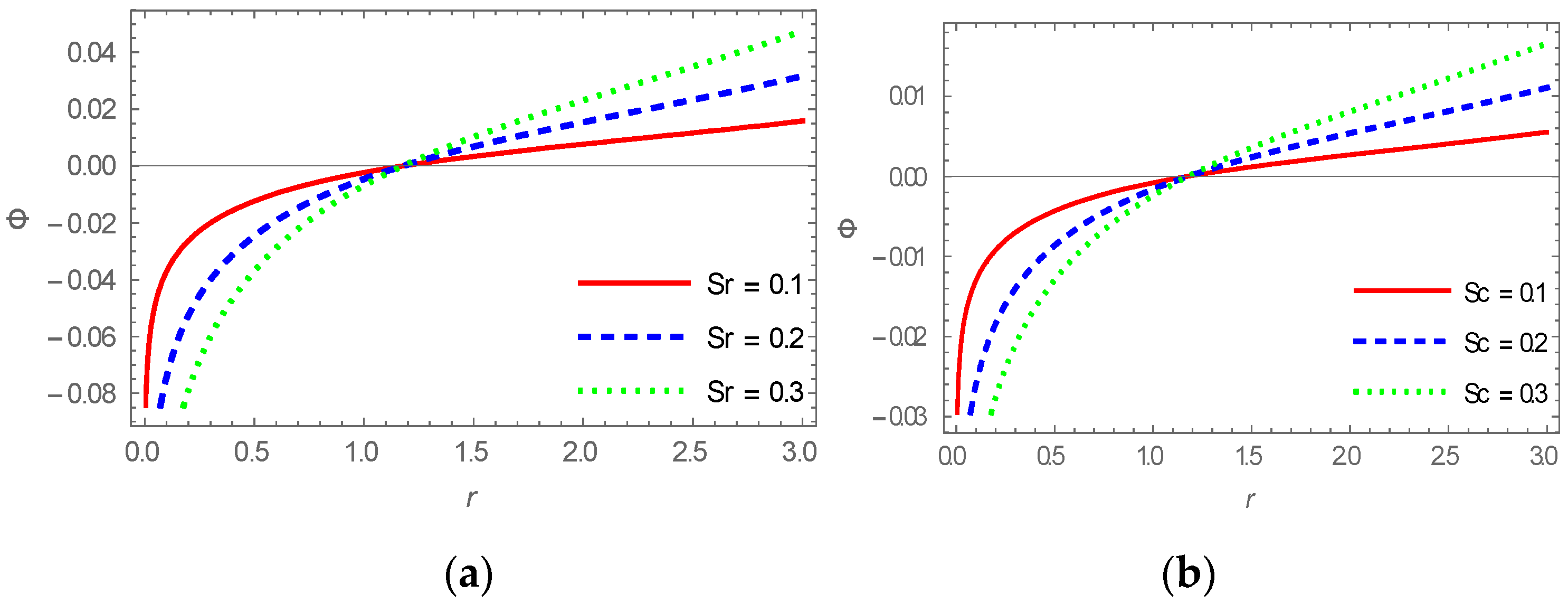
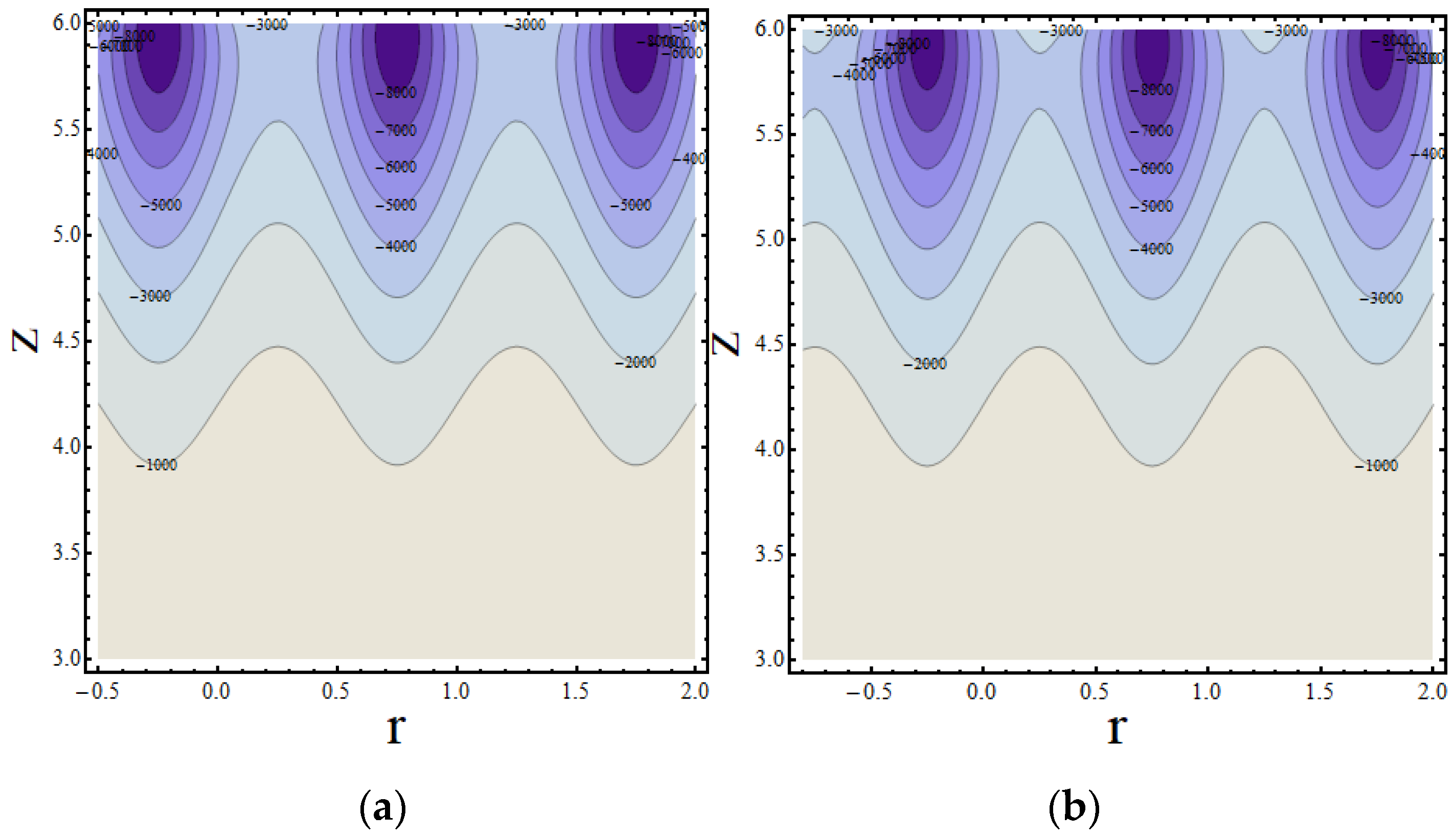
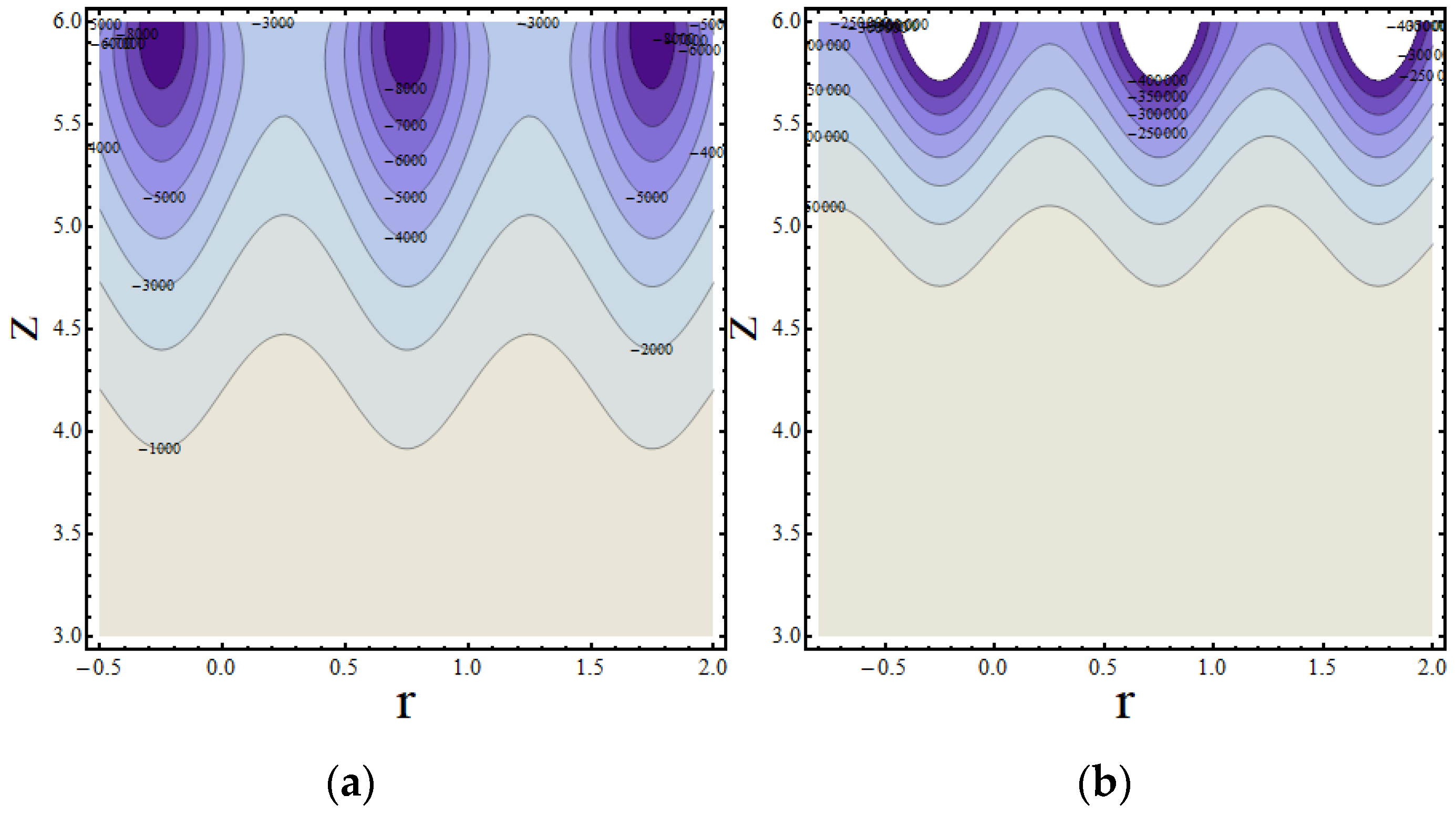
4.1. Concentration Profile

Figure 2 shows the effects of the parameters Sc and Sr on the concentration profile $\mathsf{\Phi }$. It was observed that $\mathsf{\Phi }$ decreases with the increase on Sr with $r$ in the range from 0 to 1.37622, beyond which, it increased with the increase of Sr. The curves of $\mathsf{\Phi }$ were obtained for $S_r$ = 0.1, 0.2, and 0.3 when the other parameters were constant. Figure 2b shows the effect of $S_c$ on the concentration distribution, and it is clear that $\mathsf{\Phi }$ decreased as $S_c$ increased, and also $S_c$ affected the relation between $\mathsf{\Phi }$ and r. This relation appeared approximately inverse for small values of Sc, but, for large values of Sc, $\mathsf{\Phi }$ increased with increasing, till a finite value of r (minimum value), after which it decreased. These phenomena are due to the fact that the solute diffusion in fluids is always proportional to the diffusion coefficient. Therefore, a decrease in the concentration is due to a decrease of the diffusion coefficient. The same behavior was shown for $S_c$ in Figure 2b. It can be explained by Equation (22), since both parameter are inversely proportional to the concentration. As a consequence for it recuses for higher values of Sr and Sc.

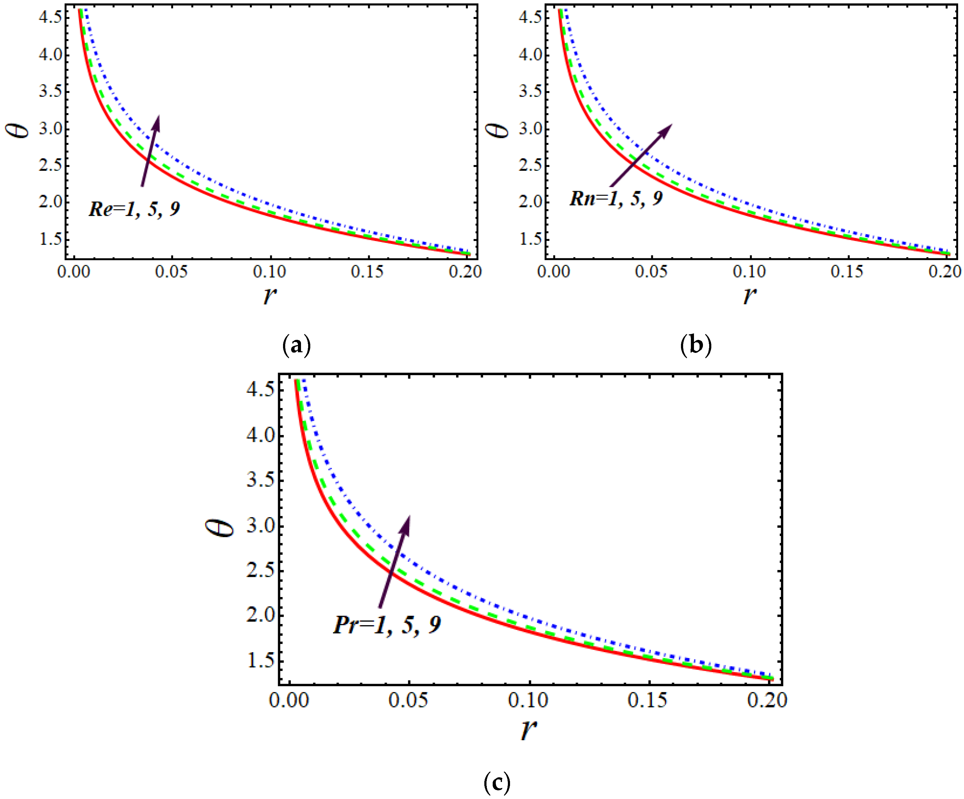
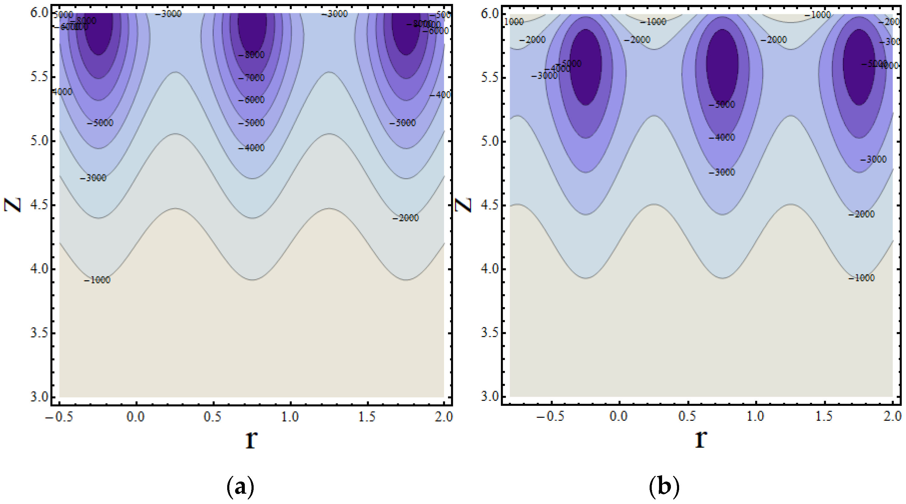
4.2. Temperature Profile

Figure 3 shows the effects of the parameters $Pr$, $Re$, and $Rn$ on the temperature profile. The graphs show that $\theta$ increased with the increase in any one of these parameters, while the others were fixed. It should be noted that for higher values of the Prandtl number, thermal conductivity was lower, which caused a reduction in conduction and boundary layer thickness. Further, the temperature increased when the radiation parameter increased. This was due to fact that the surface heat flux became large under the influence of thermal radiation, which resulted in higher temperature inside the boundary layer region. In Figure 3, the effect of $Re$, $Rn$, and $Pr$ on the temperature distribution T is displayed, and this figure shows that the temperature increased with the increasing of these parameters. The relation between T and r was approximately linear for large values of $Pr, Re, \mathrm{and} Rn>9$, but for large values of Pr (>0.7), T increased with increasing r till a finite value of r (maximum value), after which T decreased with increasing r.

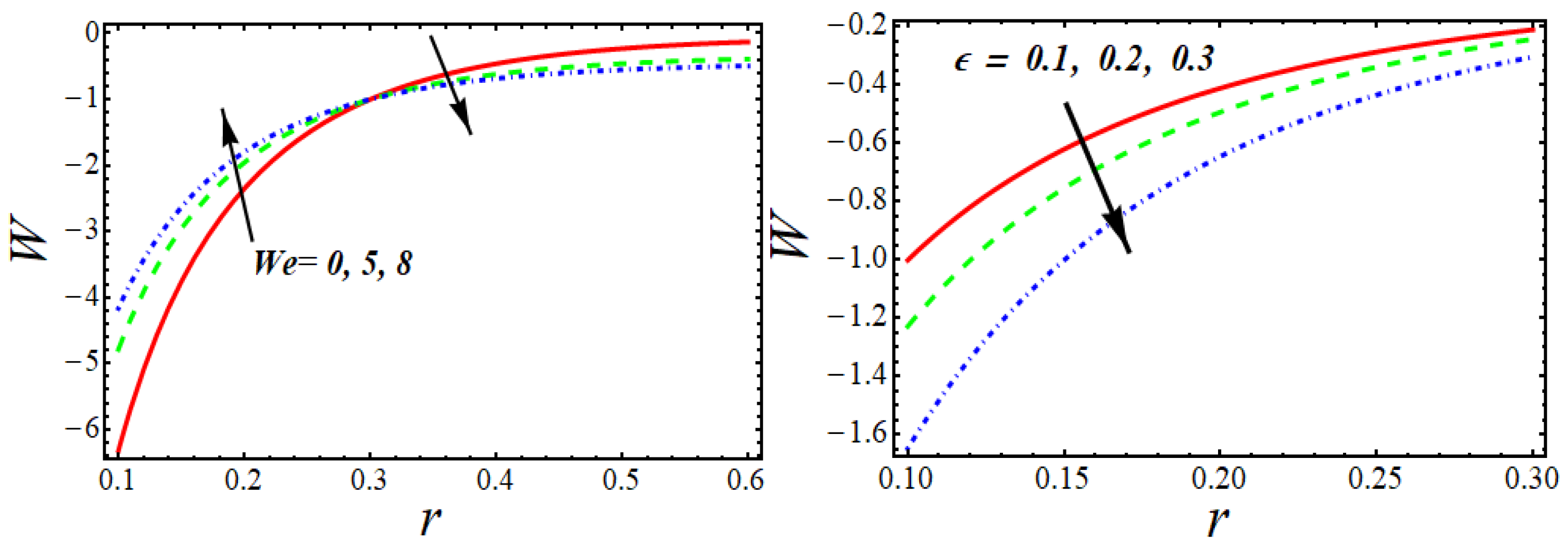
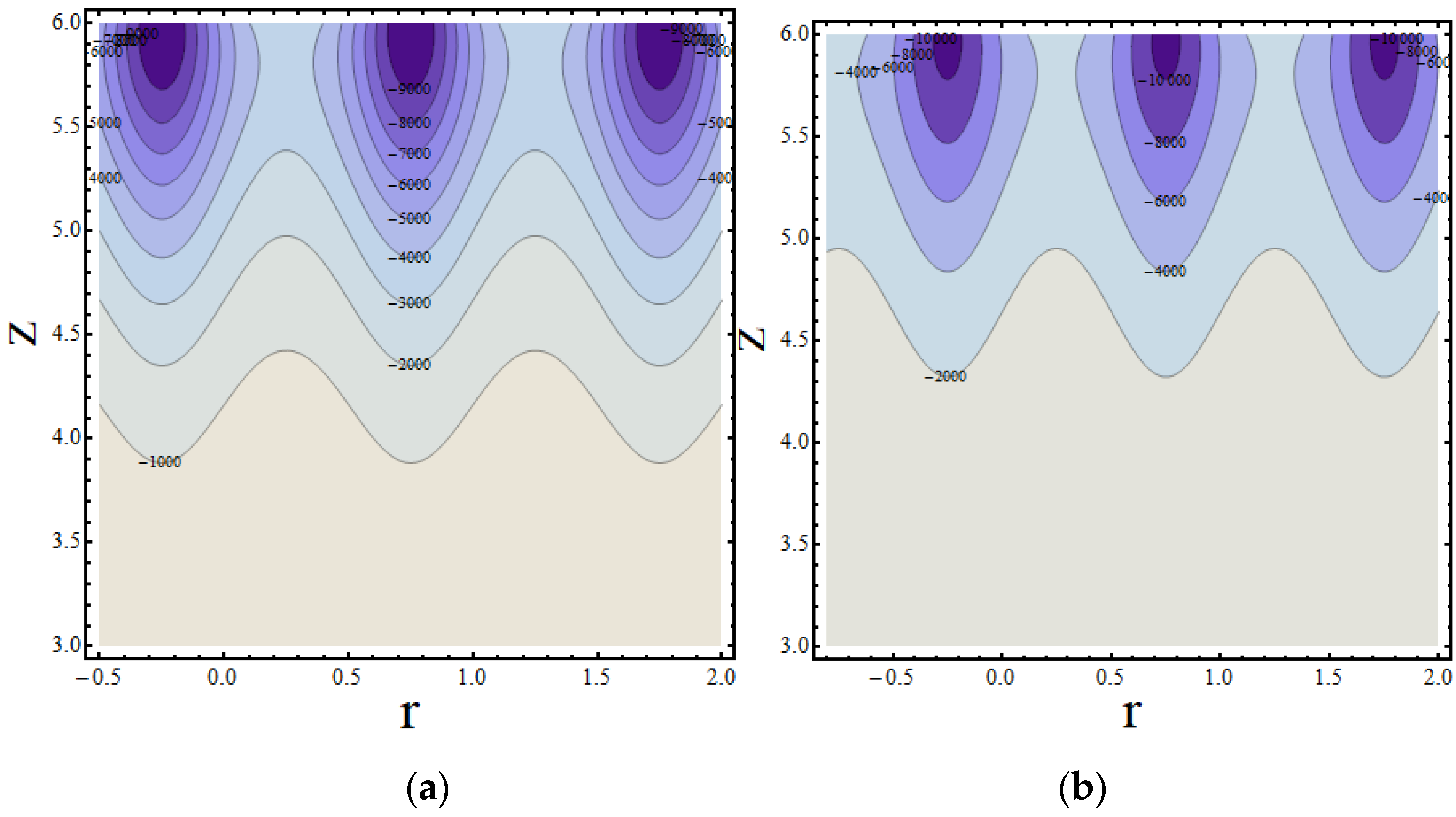
4.3. Velocity Profile

The effect of Grashof number $\left(Gc\right)$ is illustrated in Figure 4. It was observed that the fluid velocity $\left(W\right)$ decreased with the increase of $\left(Gc\right)$, and started to increase when $r \mathrm{was} 2.27$. It is seen that with the increase of $\left(Gr\right),$ the velocity $\left(W\right)$ declined, but $W$ became larger for $r>2.1726$. Figure 5 shows the variation of the velocity $\left(W\right)$ with $\left(\mathrm{r}\right)$ for various values of the Weissenberg number $\left(We\right)$. This figure shows that the fluid velocity increased with the increase of the Weissenberg number in the range of [0.1–0.32], whereas the opposite was observed in the range of [0.32–0.60]. To examine a viscoelastic flow, the Weissenberg number was used. We inspected the effect of forces from elastic to viscous. For high values of the Weissenberg number, the flow of fluid particles encountered resistance, and as a consequence, the velocity decreased. In Figure 5 we see that $\left(W\right)$ decreased with the increase of $\left(\epsilon \right)$. Figure 6 illustrates the velocity profile for various values of the magnetic and Darcy parameters. We concluded that the velocity decreased for increasing values of the magnetic field parameter $\left(M\right)$. The reason for this phenomenon is that, due to the increase in magnetic the parameters, the Lorentz force was generated and created a resistance force in the flow; as a result, the velocity profile decreased. Further, this figure shows that the velocity decreased by increasing M in the range of $0.10<r<0.27;$ ad after that, the velocity increased by increasing M. It is also clear that, in all curves in this figure, the maximum value of $\left(W\right)$ occurred at $0.23<r<0.25$. In Figure 6, the effect of $Da$ on the velocity distribution is displayed. It is clear that $\left(W\right)$ increased by increasing $Da$ in the range of $0.10<r<0.22$, and $\left(W\right)$ decreased by increasing $Da$ in the range of $0.22<r<0.30$. In this figure, we can also see that, although there was a big difference between the values of $Da$, we observed small differences between the three curves of $\left(W\right),$ which were taken at $Da=0.1, 0.5, 0.9$, when the other parameters were constant.

The effects of Grashof number $\left(Gc\right)$, Solutol Grashof number $\left(Gr\right)$, Weissenberg number $\left(We\right)$, Darcy number $\left(Da\right)$, magnetic field parameter $\left(M\right),$ and $\left(\epsilon \right)$ on trapping can be seen in Figure 7, Figure 8, Figure 9, Figure 10 and Figure 11. Trapping is basically the development of an interior circulating bolus of fluid by closed streamlines that is pushed ahead along with the peristaltic wave.

Figure 7 shows that the size of the trapped bolus increased with the increase in $Gr$, and near the upper wall, it disappeared when $Gr=4.1$. Figure 8 shows that a new region of the trapped bolus vanished at $Gc$ $=3.92$ nearby the flat wall of the channel, while the trapped bolus size increased for a large value of $Gc$.

It is observed in Figure 9 that the size of the trapped bolus declined with the enhancement of the magnetic parameter $M,$ while at $M$ $=4.82,$ a new trapped bolus appeared close to the flat wall of the channel and increased in dimension with the increase of $M$. Figure 10 reveals that close to the upper wall at $Da=3.99$, the trapped bolus vanished into a wave, while the size of the trapped bolus increased with the increase of $Da$.

It appears in Figure 11 that the size of the trapped bolus became larger for larger values of the parameter $We$, and at $We=3.9$, the trapped bolus disappeared into wave near the region of the upper wall.

Validation of the Model

The presented mathematical model was developed for non-Newtonian Williamson fluids and can be reduced to non-Newtonian fluids as $We \to 0$. In that case, we used the same model and mathematical equation previously described [30,31] for non-Newtonian fluids. For this purpose, the velocity profile for different values of magnetic parameter and Darcy number is presented in Figure 12. It can be seen from this comparison graph that the velocity decreased as M increased in the range of $0.5<r<1$. The effect of $Da$ on velocity distribution was similar. It is clear that w decreased as $Da$ increased in the range of $0.5<r<1$, and w decreased as $Da$ increased. Both results are similar to those obtained by Shabaan [30].

5. Conclusions

The magnetohydrodynamic peristaltic flow of a Williamson fluid for varying temperature, velocity, and concentration values through a porous medium was considered in this study. It is important to mention that if the current Williamson model is used in rectangular coordinates, we obtain the same results as those previously reported [23,24]. The following graphical results that we obtained with the described model are the same those as obtained by Shaban et al. [21].

• The behavior of the velocity profile was the same as the values of magnetic parameter and Da parameter increased.
• The temperature distribution was same for higher values of the Prandtl and M parameters.
• The dimensionless concentration $\varnothing$ was the same for different values of Sc and Sr

The essential features of this analysis are the following:

• For higher values of boundary layer thickness and thermal conductivity, the temperature $\theta$ increased; the relation between $\theta$ and r was approximately linear for large values of $Pr, Re, \mathrm{and} Rn>9$.
• The velocity decreased by increasing M in the range of $0.10<r<0.27;$ after that, the velocity increased by increasing M.
• The velocity decreased for higher values of the parameters $Gr$ and $Gc,$ but at $r=0.20,$ it started to increase.
• The concentration force showed a dual behavior for various values of the parameters Sc and $Sr$ because solute diffusion in fluids is always proportional to the diffusion coefficient. Therefore, a decrease in concentration field was due to a decrease in the diffusion coefficient.
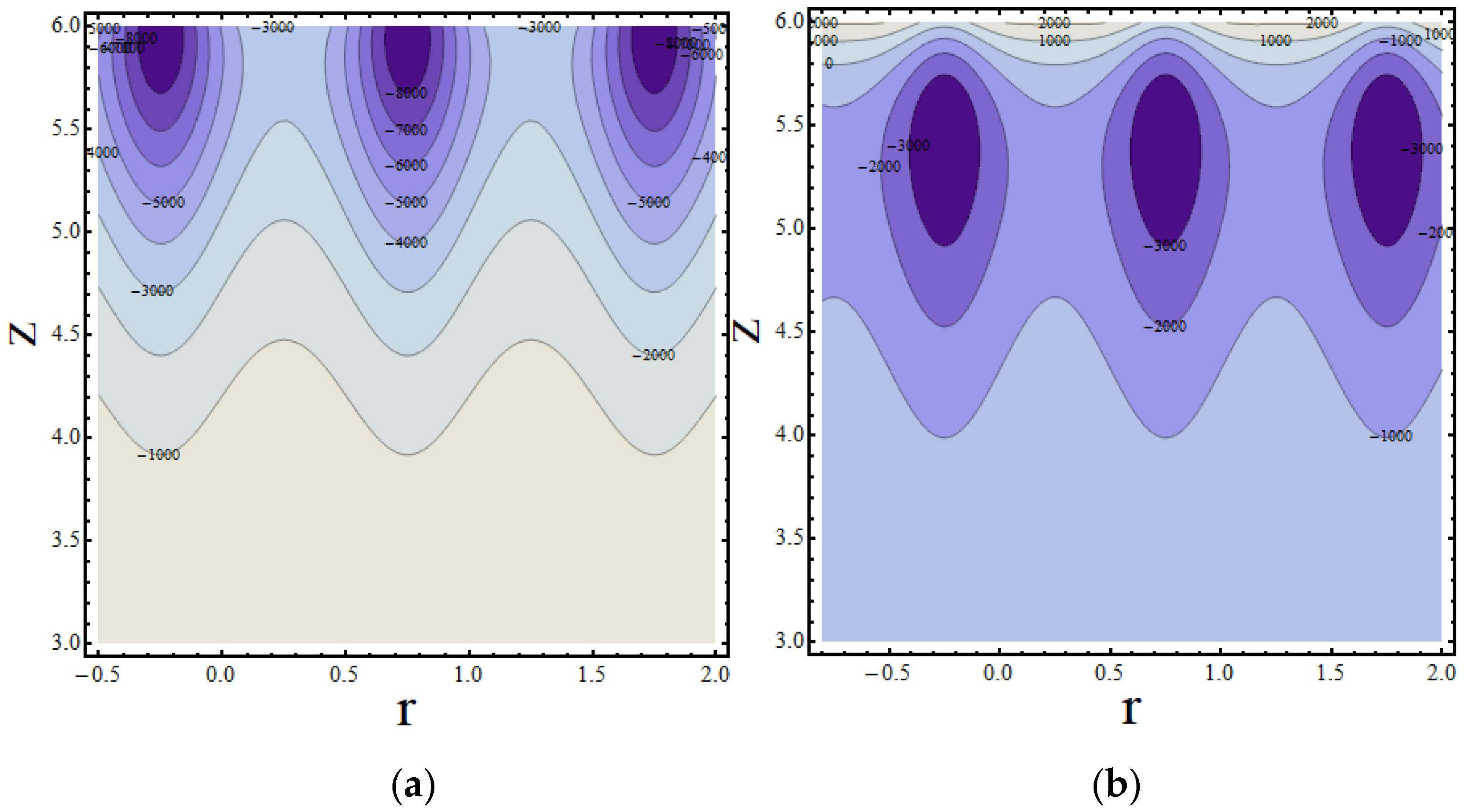
• Similar effects were observed in trapping for the parameter $Gr$, and the size of the trapped bolus decreased with the increase of $Gr$. It is further concluded that a trapped bolus developed in a new region near the flat wall of the channel and increased in size with the increase of $Gr$.
• The performance of the parameters $Da, M, Gc$, and $We$ was similar on the trap and it was revealed that near the trap, the bolus increased with the increase of $W$.

References

1. Bhatti, M.M.; Abbas, M.A.; Rashidi, M.M. Entropy generation in blood flow with heat and mass transfer for the Ellis fluid model. Heat Transf. Res. 2018, 49, 747–760. [Google Scholar] [CrossRef]
2. Bhatti, M.M.; Abbas, M.A.; Rashidi, M.M. Entropy generation for peristaltic blood flow with casson model and consideration of magnetohydrodynamics effects. Walailak J. Sci. Technol. (WJST). 2017, 14, 451–461. [Google Scholar]
3. Raza, R.; Mabood, F.; Naz, R.; Abdelsalam, S.I. Thermal transport of radiative Williamson fluid over stretchable curved surface. Therm. Sci. Eng. Prog. 2021, 23, 100887. [Google Scholar] [CrossRef]
4. Jia, Z.; Xuan, Y. Analysis on interaction among solar light and suspended nanoparticles in nanofluids. J. Quant. Spectrosc. Radiat. Transf. 2021, 269, 107692. [Google Scholar]
5. Sun, J.; Guo, L.; Jing, J.; Tang, C.; Lu, Y.; Fu, J.; Ullmann, A.; Brauner, N. Investigation on laminar pipe flow of a non-Newtonian Carreau-Extended fluid. J. Pet. Sci. Eng. 2021, 205, 108915. [Google Scholar] [CrossRef]
6. Rashid, M.; Ansar, K.; Nadeem, S. Effects of induced magnetic field for peristaltic flow of Williamson fluid in a curved channel. Phys. A Stat. Mech. Appl. 2020, 553, 123979. [Google Scholar] [CrossRef]
7. Nadeem, S.; Akram, S. Peristaltic flow of a Williamson fluid in an asymmetric channel. Communications in Nonlinear Sci. Num. Simul. 2010, 15, 1705–1716. [Google Scholar] [CrossRef]
8. Almaneea, A. Numerical study on heat and mass transport enhancement in MHD Williamson fluid via hybrid nanoparticles. Alex. Eng. J. 2022, 61, 8343–8354. [Google Scholar] [CrossRef]
9. Dadheech, A.; Parmar, A.; Agrawal, K.; Al-Mdallal, Q.; Sharma, S. Second law analysis for MHD slip flow for Williamson fluid over a vertical plate with Cattaneo-Christov heat flux. Case Stud. Therm. Eng. 2022, 33, 101931. [Google Scholar] [CrossRef]
10. Asjad, M.I.; Zahid, M.; Inc, M.; Baleanu, D.; Almohsen, B. Impact of activation energy and MHD on Williamson fluid flow in the presence of bioconvection. Alex. Eng. J. 2022, 61, 8715–8727. [Google Scholar] [CrossRef]
11. Shashikumar, N.; Madhu, M.; Sindhu, S.; Gireesha, B.; Kishan, N. Thermal analysis of MHD Williamson fluid flow through a microchannel. Int. Commun. Heat Mass Transf. 2021, 127, 105582. [Google Scholar] [CrossRef]
12. Bhatti, M.M.; Rashidi, M.M.; Abbas, M.A. Analytic Study of Drug Delivery in Peristaltically Induced Motion of Non-Newtonian Nanofluid. J. Nanofluids 2016, 5, 920–927. [Google Scholar] [CrossRef]
13. Abbas, M.A.; Bai, Y.; Rashidi, M.M.; Bhatti, M.M. Analysis of Entropy Generation in the Flow of Peristaltic Nanofluids in Channels with Compliant Walls. Entropy 2016, 18, 90. [Google Scholar] [CrossRef]
14. Sinha, A.; Shit, G.C.; Ranjit, N.K. Peristaltic transport of MHD flow and heat transfer in an asymmetric channel: Effects of variable viscosity, velocity-slip and temperature jump. Alex. Eng. J. 2015, 54, 691–704. [Google Scholar] [CrossRef] [Green Version]
15. Saleem, A.; Akhtar, S.; Alharbi, F.M.; Nadeem, S.; Ghalambaz, M.; Issakhov, A. Physical aspects of peristaltic flow of hybrid nano fluid inside a curved tube having ciliated wall. Results Phys. 2020, 19, 103431. [Google Scholar] [CrossRef]
16. Riaz, A.; Bhatti, M.M.; Ellahi, R.; Zeeshan, A.; Sait, S.M. Mathematical Analysis on an Asymmetrical Wavy Motion of Blood under the Influence Entropy Generation with Convective Boundary Conditions. Symmetry 2020, 12, 102. [Google Scholar] [CrossRef] [Green Version]
17. Abbas, M.A.; Bég, O.A.; Zeeshan, A.; Hobiny, A.; Bhatti, M.M. Parametric analysis and minimization of entropy generation in bioinspired magnetized non-Newtonian nanofluid pumping using artificial neural networks and particle swarm optimization. Therm. Sci. Eng. Prog. 2021, 24, 100930. [Google Scholar] [CrossRef]
18. Afifi, N.A.S. Study of Peristaltic Flow for Different Cases. Ph.D. Thesis, Ain Shams University, Cairo, Egypt, 1998. [Google Scholar]
19. Bhatti, M.M.; Abbas, M.A. Simultaneous effects of slip and MHD on peristaltic blood flow of Jeffrey fluid model through a porous medium. Alex. Eng. J. 2016, 55, 1017–1023. [Google Scholar] [CrossRef] [Green Version]
20. Noreen, S.; Tripathi, D. Heat transfer analysis on electroosmotic flow via peristaltic pumping in non-Darcy porous medium. Therm. Sci. Eng. Prog. 2019, 11, 254–262. [Google Scholar] [CrossRef]
21. Pattnaik, P.K.; Parida, S.K.; Mishra, S.R.; Abbas, M.A.; Bhatti, M.M. Analysis of Metallic Nanoparticles (Cu, Al2O3, and SWCNTs) on Magnetohydrodynamics Water-Based Nanofluid through a Porous Medium. J. Math. 2022, 2022, 3237815. [Google Scholar] [CrossRef]
22. Hareli, S.; Nave, O.; Gol’dshtein, V. The Evolutions in Time of Probability Density Functions of Poly dispersed Fuel Spray—The Continuous Mathematical Model. Appl. Sci. 2021, 11, 9739. [Google Scholar] [CrossRef]
23. Yang, M.; Abbas, M.A.; Khudair, W.S. Energy and Temperature-Dependent Viscosity Analysis on Magnetized Eyring-Powell Fluid Oscillatory Flow in a Porous Channel. Energies 2021, 14, 7829. [Google Scholar] [CrossRef]
24. Nawaz, M.; Sadiq, M.A. Unsteady heat transfer enhancement in Williamson fluid in Darcy-Forchheimer porous medium under non-Fourier condition of heat flux. Case Stud. Therm. Eng. 2021, 28, 101647. [Google Scholar] [CrossRef]
25. Hayat, T.; Saleem, A.; Tanveer, A.; Alsaadi, F. Numerical study for MHD peristaltic flow of Williamson nanofluid in an endoscope with partial slip and wall properties. Int. J. Heat Mass Transf. 2017, 114, 1181–1187. [Google Scholar] [CrossRef]
26. Bhatti, M.M.; Arain, M.B.; Zeeshan, A.; Ellahi, R.; Doranehgard, M.H. Swimming of Gyrotactic Microorganism in MHD Williamson nanofluid flow between rotating circular plates embedded in porous medium: Application of thermal energy storage. J. Energy Storage 2022, 45, 103511. [Google Scholar] [CrossRef]
27. Li, Y.-X.; Alshbool, M.H.; Lv, Y.-P.; Khan, I.; Khan, M.R.; Issakhov, A. Heat and mass transfer in MHD Williamson nanofluid flow over an exponentially porous stretching surface. Case Stud. Therm. Eng. 2021, 26, 100975. [Google Scholar] [CrossRef]
28. Ahmed, K.; Akbar, T.; Muhammad, T.; Alghamdi, M. Heat transfer characteristics of MHD flow of Williamson nanofluid over an exponential permeable stretching curved surface with variable thermal conductivity. Case Stud. Therm. Eng. 2021, 28, 101544. [Google Scholar] [CrossRef]
29. Salmi, A.; Madkhali, H.A.; Nawaz, M.; Alharbi, S.O.; Alqahtani, A. Numerical study on non-Fourier heat and mass transfer in partially ionized MHD Williamson hybrid nanofluid. Int. Commun. Heat Mass Transf. 2022, 133, 105967. [Google Scholar] [CrossRef]
30. Shaaban, A.A.; Abou-Zeid, M.Y. Effects of Heat and Mass Transfer on MHD Peristaltic Flow of a Non-Newtonian Fluid through a Porous Medium between Two Coaxial Cylinders. Math. Probl. Eng. 2013, 2013, 819683. [Google Scholar] [CrossRef]
31. Eldabe, N.T.; Mohamed, Y.A. Magnetohydrodynamic peristaltic flow with heat and mass transfer of mi-cropolar biviscosity fluid through a porous medium between two co-axial tubes. Arab. J. Sci. Eng. 2014, 39, 5045–5062. [Google Scholar] [CrossRef]
32. Khudair, W.S.; Dheia Gaze, S.A. Influence of Heat Transfer on MHD Oscillatory Flow for Williamson Fluid with Variable Viscosity through a Porous Medium. Int. J. Fluid Mech. Therm. Sci. 2018, 4, 11–17. [Google Scholar] [CrossRef] [Green Version]
33. Wissam, S.K.; Al-Khafajy, D.G. Influence of heat transfer on Magneto hydrodynamics oscillatory flow for Williamson fluid through a porous medium. Iraqi J. Sci. 2018, 59, 389–397. [Google Scholar]
Figure 1. Geometry of the flow.
Symmetry 14 00953 g001
Figure 2. The variation of the concentration Φ vs. r at Ω = 1 , R e = 3 , P r = 2 , R n = 0.5 , = 0.3 , ϵ = 0.3 , i = 1 , z = 0.1 for: (a) S c = 0.1 (b) S r = 0.07 .
Symmetry 14 00953 g002
Figure 3. The variation of the temperature θ vs. r, at Ω = 1 , P r = 2 ,   ϵ = 0.3 , = 0.3 , z = 0.1 . (a) Pr = 2, Rn = 2 (b) Re = 0.1, Pr = 2, (c) Re = 0.1, Rn = 2.
Symmetry 14 00953 g003
Figure 4. Velocity profile for G c and G r with Ω = 1 , ϵ = 0.2 , ϕ = 0.5 , W e = 1 , R e = 2 , P r = 2 , R n = 2 , p z = 1.5 , S c = 0.5 ,   S r = 0.07 , M = 1 , D a = 0.8 , ξ = π 4 .
Symmetry 14 00953 g004
Figure 5. Velocity profile for W e and ϵ with Ω = 1 , G c = 1 , ϕ = 0.5 , G r = 1 , R e = 2 , P r = 2 , R n = 2 , p z = 1.5 , S c = 0.5 ,   S r = 0.07 , M = 1 , D a = 0.8 , ξ = π 4 .
Symmetry 14 00953 g005
Figure 6. Velocity profile for M and D a with Ω = 1 , ϵ = 0.2 , ϕ = 0.5 , W e = 1 , R e = 2 , P r = 2 , R n = 2 , p z = 1.5 , S c = 0.5 , S r = 0.07 , G c = 1 , G r = 1 , ξ = π 4 .
Symmetry 14 00953 g006
Figure 7. Streamlines in the wave frame for various values of G r when Ω = 0.9 , ϵ = 0.3 , ϕ = 0.1 , W e = 0.1 , R e = 1 , R n = 2 , P r = 2 , S c = 0.5 , S r = 0.1 , G c = 0.1 , M = 1.1 , D a = 0.9 , ξ = π 4 ; ( a )   G r = 0.1 ,   ( b )   G r = 0.2 .
Symmetry 14 00953 g007
Figure 8. Streamlines in the wave frame for various values of G c when ϕ = 0.1 , ϵ = 0.3 , W e = 0.1 ,   Ω = 0.9 , R e = 1 , R n = 2 , P r = 2 , S c = 0.5 , S r = 0.1 , G r = 2 , M = 1.1 , D a = 0.9 , ξ = π 4 ; ( a )   G c = 3 ,   ( b )   G c = 3.5 .
Symmetry 14 00953 g008
Figure 9. Streamlines in the wave frame for various values of M when ϕ = 0.1 , ϵ = 0.3 , W e = 0.1 , R e = 1 , R n = 2 , P r = 2 , S c = 0.5 , S r = 0.1 , G c = 0.1 , G r = 2 , D a = 0.9 , ξ = π 4 ; ( a )   M = 0.1 ,   ( b )   M = 0.2 .
Symmetry 14 00953 g009
Figure 10. Streamlines in the wave frame for various values of W e when ϵ = 0.3 , M = 1.1 , R e = 1 , R n = 2 , Ω = 0.9 , P r = 2 , ϕ = 0.1 , S c = 0.5 , S r = 0.1 , D a = 0.9 , G r = 2 , G c = 0.1 , ξ = π 4 ; ( a )   W e = 0.3 ,   ( b )   W e = 0.4 .
Symmetry 14 00953 g010
Figure 11. Streamlines in the wave frame for various values of ϵ when D a = 0.9 , R n = 2 , ϕ = 0.1 , W e = 0.1 , Ω = 0.9 , R e = 1 , P r = 2 , S c = 0.5 , S r = 0.1 ,   G r = 2 , G r = 2 , M = 1 , ξ = π 4 ; ( a )   ϵ = 0.2 ,   ( b )   ϵ = 0.3 .
Symmetry 14 00953 g011
Figure 12. Graphical results of the Velocity Profile against Magnetic parameter and Darcy number for a non-Newtonian fluid ( W e   0 ).
Symmetry 14 00953 g012