Type II Half-Logistic Odd Fréchet Class of Distributions: Statistical Theory and Applications

Abstract

A new class of statistical distributions called the Type II half-Logistic odd Fréchet-G class is proposed. The new class is a continuation of the unusual Fréchet class. This class is analytically feasible and could be used to evaluate real-world data effectively. The new suggested class of distributions has many new symmetrical and asymmetrical sub-models. We propose new four sub-models from the new class of distributions which are called Type II half-Logistic odd Fréchet exponential distribution, Type II half-Logistic odd Fréchet Rayleigh distribution, Type II half-Logistic odd Fréchet Weibull distribution, and Type II half-Logistic odd Fréchet Lindley distribution. Some statistical features of Type II half-Logistic odd Fréchet-G class such as ordinary moments (ORMs), incomplete moments (INMs), moment generating function (MGEF), residual life (REL), and reversed residual life (RREL) functions, and Rényi entropy (RéE) are derived. Six methods of estimation such as maximum likelihood, least-square, a maximum product of spacing, weighted least square, Cramér-von Mises, and Anderson–Darling are produced to estimate the parameters. To test the six estimation methods’ performance, a simulation study is conducted. Four real-world data sets are utilized to highlight the importance and applicability of the proposed method.

1. Introduction

Today, there is a need for mathematical models required to retrieve all of the information from data and the ability to engage with it and make it usable in engineering, biological study, economics, and environmental sciences, to name a few examples. A lot of generations of academics have so far concentrated their efforts to build larger classes of distributions. The classic strategy consists of adding (parameters) to a scale or shape to the baseline model, also through the use of special functions (beta, gamma, excessive geometry, etc.), which makes the resulting distribution more adaptable, which is useful for understanding the behavior of density shapes and hazard rate shapes, for checking the goodness of fit of proposed distributions, or the flexibility on some important modeling aspects such as mean E(X), variance V(X), distribution tails, skewness (SK), kurtosis (KU), etc. Consequently, new different classes of continuous distributions have been offered, including those produced in the statistical literature listed below. Some well-known classes are the Fréchet class defined in [1], Marshall–Olkin class given in [2], beta-class given in [3], the generalized log-logistic class given in [4], the odd exponentiated half logistic (HL) class given in [5], the generalized odd log-logistic class given in [6], the Type I HL class given in [7], the logistic-X class given in [8], generalized odd log-logistic class given in [9], Kumaraswamy Type I HL class given in [10], the transmuted odd Fréchet ($OF$)-class given in [11], extended $OF$-G class given in [12], transmuted geometric-G [13], odd Perks-G class [14], odd Lindley-G in [15], truncated Cauchy power Weibull-G [16], generalized transmuted-G [17], truncated Cauchy power-G in [18], Burr X-G (BX-G) class [19], odd inverse power generalized Weibull-G [20], Type II exponentiated half-Logistic-G in [21], Topp Leone -G in [22], exponentiated M-G by [23], odd Nadarajah–Haghighi-G in [24], exponentiated truncated inverse Weibull-G in [25], T-X generator proposed in [26], among others.

Several Fréchet classes have been judged successful in a variety of statistical applications in the last years as [27] proposed a four-parameter model named the exponential transmuted Fréchet distribution, which extends the Fréchet distribution. Ref [1] proposed the $OF-G$ class of distributions with distribution function (cdf) and density function (pdf), respectively, are follows, for $x>0$

$$G_{{}_{O{F}_r}}(x;\theta )=e^{-{\left(\frac{\overline{G}(x,\phi )}{G(x,\phi )}\right)}^{\theta }},$$

(1)

and

$$g_{{}_{O{F}_r}}(x;\theta )=\frac{\theta g(x,\phi ){\left(1-G(x,\phi )\right)}^{\theta -1}}{G{(x,\phi )}^{\theta +1}}{e}^{-{\left(\frac{\overline{G}(x,\phi )}{G(x,\phi )}\right)}^{\theta }},$$

(2)

where $\theta$$>0$ is a shape parameter, $G(x,\phi )$ and $g(x,\phi )$ are the pdf and cdf of a baseline continuous distribution with $\phi$ as parameter vector, respectively.

The $OF-G$ class was successfully considered in various statistical applications over the last few years. This reputation can be explained by its simple and versatile exponential-odd form, with the use of just one additional parameter, very different from the other current families. Ref [28] represented a new class of continuous distributions with an extra scale parameter $\alpha >0$ called the Type II HL-G ($TIIHL-G)$ class. The cdf and pdf of the $TIIHL-G$ class of distributions, respectively, are provided by

$$F\left(x\right)=\frac{2{\left[G\left(x\right)\right]}^{\alpha }}{1+{\left[G\left(x\right)\right]}^{\alpha }},$$

(3)

and

$$f\left(x\right)=2\alpha g\left(x\right){\left[G\left(x\right)\right]}^{\alpha -1}{\left[1+{\left[G\left(x\right)\right]}^{\alpha }\right]}^{-2}.$$

(4)

The failure (hazard) rate function (hrf) is defined by

$$\tau \left(x\right)=\frac{2\alpha g\left(x\right){\left[G\left(x\right)\right]}^{\alpha -1}}{1-{\left[G\left(x\right)\right]}^{2\alpha }}.$$

(5)

In this paper, we discuss a new extension of the odd Fréchet-G class for a given baseline distribution with cdf $G(x,\phi )$ using the Type II HL generator and this class is called the Type II HL odd Fréchet-G$(TIIHLOF-G)$ class of distributions. This new suggested class of distributions is very flexible and has many new symmetrical and asymmetrical sub-models. The cdf of $(TIIHLOF-G)$ class is obtained by inserting Equation (1) in Equation (3), we get

$$F(x,\alpha ,\theta ,\phi )=\frac{2e^{-\alpha {\left(\frac{\overline{G}(x,\phi )}{G(x,\phi )}\right)}^{\theta }}}{1+e^{-\alpha {\left(\frac{\overline{G}(x,\phi )}{G(x,\phi )}\right)}^{\theta }}},x>0.$$

(6)

For each baseline G, the $TIIHLOF-G$ cdf is given by Equation (6). The corresponding pdf is

$$f(x;\alpha ,\theta ,\phi )=\frac{2\alpha \theta g(x,\phi )\overline{G}{(x,\phi )}^{\theta -1}}{G{(x,\phi )}^{\theta +1}}{e}^{-\alpha {\left(\frac{\overline{G}(x,\phi )}{G(x,\phi )}\right)}^{\theta }}{\left[1+e^{-\alpha {\left(\frac{\overline{G}(x,\phi )}{G(x,\phi )}\right)}^{\theta }}\right]}^{-2}.$$

(7)

The hrf of $TIIHLOF-G$ class is provided by

$$\chi \left(x\right)=\frac{2\alpha \theta g(x,\phi )\overline{G}{(x,\phi )}^{\theta -1}{e}^{-\alpha {\left(\frac{\overline{G}(x,\phi )}{G(x,\phi )}\right)}^{\theta }}}{G{(x,\phi )}^{\theta +1}\left[1-e^{-2\alpha {\left(\frac{\overline{G}(x,\phi )}{G(x,\phi )}\right)}^{\theta }}\right]}.$$

The $TIIHLOF-G$ quantile function (qf) is given below

$$F^{-1}\left(u\right)=Q_G\left(u\right)=G^{-1}\left[\frac{1}{1+{\left\{\frac{-1}{\alpha }log\left(\frac{u}{2-u}\right)\right\}}^{\frac{1}{\theta }}}\right].$$

(8)

The fundamental goal of the article under consideration is to introduce a new class of statistical distributions called the Type II half-Logistic odd Fréchet-G class (TIIHLOF-G for short) as well as to investigate its statistical characteristics. The following points provide sufficient incentive to study the proposed class of distributions. We specify it as follows: (i) the new class of distributions are very flexible and have many new symmetrical and asymmetrical sub-models; (ii) it is remarkable to observe the flexibility of the proposed family with the diverse graphical shapes of probability density functions (pdf) and hazard rate functions (hrf). So, the form analysis of the corresponding pdf and hrf has shown new characteristics, revealing the unseen fitting potential of the TIIHLOF-G; (iii) the new suggested class has a closed form of the quantile function; (iv) six methods of estimation are proposed to assess the behavior of the parameters; (v) the TIIHLOF-G is very flexible and applicable. This ability of the new class is explored using four real-life data sets proving the practical utility of the model being featured.

The substance of the article is arranged as follows: Section 2 presents a linear representation of the $TIIHLOF-G$ class density. Four new sub-models are provided in Section 3. Section 4 contains a number of statistical features such as ORMs, INMs, MGEF, REL, and RREL functions, and RéE. In Section 5, different estimation methods of the model parameters are determined. Section 6 shows simulation results. Section 7 investigates three real-world data sets to demonstrate the flexibility and potential of the $TIIHLOF-G$ class using the $TIIHLOFExp$ and $TIIHLOFW$ distributions. Finally, in Section 8, the conclusions are offered.

2. Useful Expansion

Assuming $\mid z\mid <1$ and $b>0$ be a real non-integer, then the next binomial expansions occur.

$${(1+z)}^{-b}=\sum _{k=0}^{\infty }{(-1)}^k\frac{\Gamma (b+k)}{k!\Gamma \left(b\right)}{z}^k.$$

(9)

Applying Equation (9) to the last term in Equation (7), then

$$f_{TIIHLOF-G}\left(x\right)=\frac{2\alpha \theta g(x,\phi )\overline{G}{(x,\phi )}^{\theta -1}}{G{(x,\phi )}^{\theta +1}}\sum _{i=0}^{\infty }(i+1)e^{-\alpha (i+1){\left(\frac{\overline{G}(x,\phi )}{G(x,\phi )}\right)}^{\theta }}.$$

(10)

The exponential function’s power series now yields

$$e^{-\alpha (i+1){\left(\frac{\overline{G}(x,\phi )}{G(x,\phi )}\right)}^{\theta }}=\sum _{j=0}^{\infty }\frac{{(-1)}^j{\alpha }^j{(i+1)}^j}{j!}\frac{\overline{G}{(x,\phi )}^{\theta j}}{G{(x,\phi )}^{\theta j}}.$$

(11)

Inserting Equation (11) in Equation (10), then

$$f_{TIIHLOF-G}\left(x\right)=g(x,\phi )\sum _{i,j=0}^{\infty }\frac{2\theta {(-1)}^j{\alpha }^{j+1}{(i+1)}^{j+1}}{j!}\frac{\overline{G}{(x,\phi )}^{\theta (j+1)-1}}{G{(x,\phi )}^{\theta (j+1)+1}},$$

(12)

using the generalized binomial expansion to ${(1-G(x;\phi ))}^{-\left[\theta (j+1)+1\right]}$,

$${(1-G(x;\phi ))}^{-\left[\theta (j+1)+1\right]}=\sum _{k=0}^{\infty }\frac{\Gamma \left(\theta \right(j+1)+k+1)}{k!\Gamma \left(\theta \right(j+1)+1)}G{(x;\phi )}^k,$$

(13)

and

$${(1-G(x;\phi ))}^{\left[\theta (j+1)+k+1\right]}=\sum _{d=0}^{\infty }{(-1)}^d\left(\genfrac{}{}{0pt}{}{\theta (j+1)+k+1}{d}\right)G{(x;\phi )}^d.$$

(14)

The $TIIHLOF$ pdf is an endless combination of exp-G pdfs

$$f_{TIIHLOF-G}\left(x\right)=\sum _{d=0}^{\infty }{\varpi }_d{h}_{(d+1)}\left(x\right),$$

(15)

where

$${\varpi }_d=\sum _{i,j,k=0}^{\infty }\frac{2\theta {(-1)}^{j+d}{\alpha }^{j+1}{(i+1)}^{j+1}\Gamma (\theta (j+1)+k+1)}{j!k!\Gamma \left(\theta \right(j+1)+1)(d+1)}\left(\genfrac{}{}{0pt}{}{\theta (j+1)+k+1}{d}\right),$$

and $h_{(d+1)}\left(x\right)=(d+1)g\left(x\right)G^d\left(x\right)$.

3. Submodels of the TIIHLOF-G Class

We exhibit four sub-models of the $TIIHLOF-G$ distribution class.

3.1. Type II Half-Logistic Odd Fréchet Exponential (TIIHLOFExp) Distribution

Let $G\left(x\right)$ and $g\left(x\right)$ in Equations (6) and (7) be the cdf and pdf of Exp distribution where $G(x;\phi )=1-e^{-\lambda x}$ and $g(x;\phi )=$$\lambda e^{-\lambda x}.$ The cdf and pdf of Type II half-Logistic odd Fréchet Exp ($TIIHLOFExp$) are given below

$$F\left(x\right)=\frac{2e^{-\alpha {\left(\frac{e^{-\lambda x}}{1-e^{-\lambda x}}\right)}^{\theta }}}{1+e^{-\alpha {\left(\frac{e^{-\lambda x}}{1-e^{-\lambda x}}\right)}^{\theta }}},x>0,$$

and

$$f\left(x\right)=\frac{2\alpha \theta \lambda e^{-\lambda x}{\left(e^{-\lambda x}\right)}^{\theta -1}}{{(1-e^{-\lambda x})}^{\theta +1}}{e}^{-\alpha {\left(\frac{e^{-\lambda x}}{1-e^{-\lambda x}}\right)}^{\theta }}{\left[1+e^{-\alpha {\left(\frac{e^{-\lambda x}}{1-e^{-\lambda x}}\right)}^{\theta }}\right]}^{-2}.$$

Figure 1 describes the different forms of the pdf of TIIHLOFExp distribution.

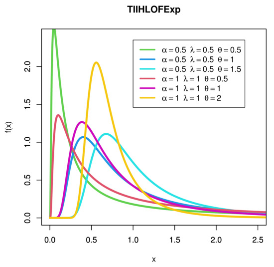
Figure 1. Shapes of the pdf of TIIHLOFExp $(\alpha ,\lambda ,\theta )$ for various values of parameter.

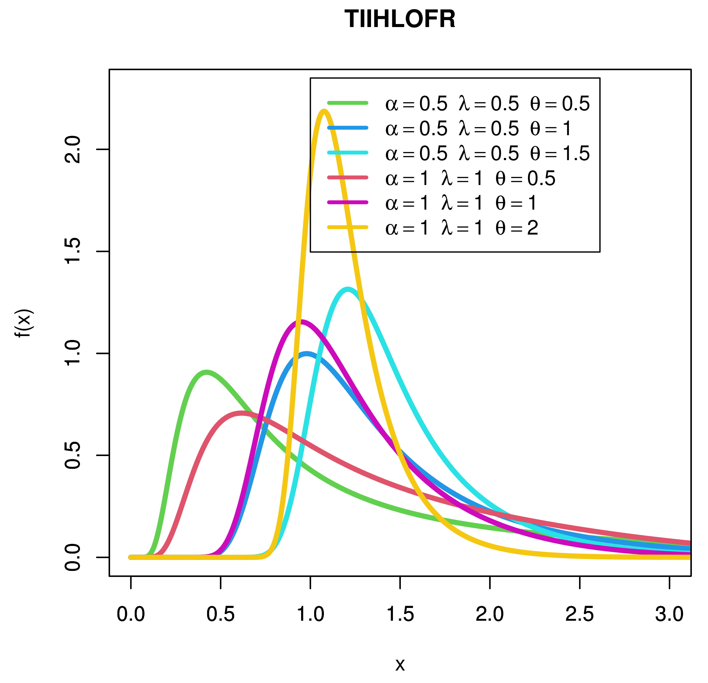
3.2. Type II Half-Logistic Odd Fréchet Rayleigh (TIIHLOFR) Distribution

Here we take $G\left(x\right)=1-e^{-\frac{\lambda }{2}{x}^2}$ and $g(x;\phi )=\lambda x{e}^{-\frac{\lambda }{2}{x}^2}$ be the Rayleigh distribution. The cdf and pdf of $TIIHLOFR$ model, are given below

$$F\left(x\right)=\frac{2e^{-\alpha {\left(\frac{e^{-\frac{\lambda }{2}{x}^2}}{1-e^{-\frac{\lambda }{2}{x}^2}}\right)}^{\theta }}}{1+e^{-\alpha {\left(\frac{e^{-\frac{\lambda }{2}{x}^2}}{1-e^{-\frac{\lambda }{2}{x}^2}}\right)}^{\theta }}},x>0,$$

and

$$f\left(x\right)=\frac{2\alpha \theta \lambda x{e}^{-\frac{\lambda }{2}{x}^2}{\left(e^{-\frac{\lambda }{2}{x}^2}\right)}^{\theta -1}}{{(1-e^{-\frac{\lambda }{2}{x}^2})}^{\theta +1}}{e}^{-\alpha {\left(\frac{e^{-\frac{\lambda }{2}{x}^2}}{1-e^{-\frac{\lambda }{2}{x}^2}}\right)}^{\theta }}{\left[1+e^{-\alpha {\left(\frac{e^{-\frac{\lambda }{2}{x}^2}}{1-e^{-\frac{\lambda }{2}{x}^2}}\right)}^{\theta }}\right]}^{-2}.$$

Figure 2 describes the different forms of the pdf of $TIIHLOFR$ distribution.

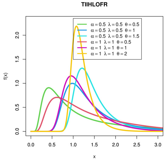
Figure 2. Shapes of the pdf of TIIHLOFR $(\alpha ,\beta ,\theta )$ for various values of parameter.

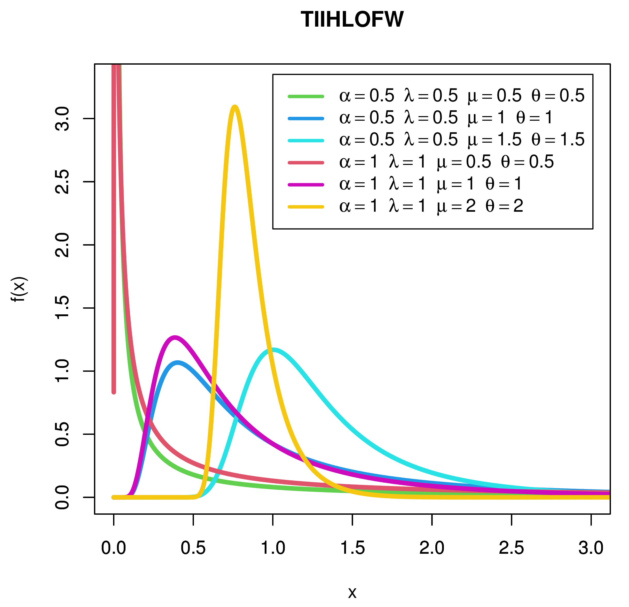
3.3. Type II Half-Logistic Odd Fréchet Weibull (TIIHLOFW) Distribution

Let $G\left(x\right)$ and $g\left(x\right)$ in Equations (6) and (7) be the cdf and pdf of Weibull distribution, where $G(x;\phi )=1-e^{-{\left(\lambda x\right)}^{\mu }}$ and $g(x;\phi )=\mu {\lambda }^{\mu }{x}^{\mu -1}$$e^{-{\left(\lambda x\right)}^{\mu }}.$ The cdf and pdf of ($TIIHLOFW$) distribution are given below

$$F\left(x\right)=\frac{2e^{-\alpha {\left(\frac{e^{-{\left(\lambda x\right)}^{\mu }}}{1-e^{-{\left(\lambda x\right)}^{\mu }}}\right)}^{\theta }}}{1+e^{-\alpha {\left(\frac{e^{-{\left(\lambda x\right)}^{\mu }}}{1-e^{-{\left(\lambda x\right)}^{\mu }}}\right)}^{\theta }}},x>0,$$

and

$$f\left(x\right)=\frac{2\alpha \theta \mu {\lambda }^{\mu }{x}^{\mu -1}{e}^{-\theta {\left(\lambda x\right)}^{\mu }}}{{(1-e^{-{\left(\lambda x\right)}^{\mu }})}^{\theta +1}}{e}^{-\alpha {\left(\frac{e^{-{\left(\lambda x\right)}^{\mu }}}{1-e^{-{\left(\lambda x\right)}^{\mu }}}\right)}^{\theta }}{\left[1+e^{-\alpha {\left(\frac{e^{-{\left(\lambda x\right)}^{\mu }}}{1-e^{-{\left(\lambda x\right)}^{\mu }}}\right)}^{\theta }}\right]}^{-2}.$$

Figure 3 describes the different forms of the pdf of TIIHLOFW distribution.

Figure 3. Shapes of the pdf of TIIHLOFW $(\alpha ,\lambda ,\mu ,\theta )$ for various values of parameter.

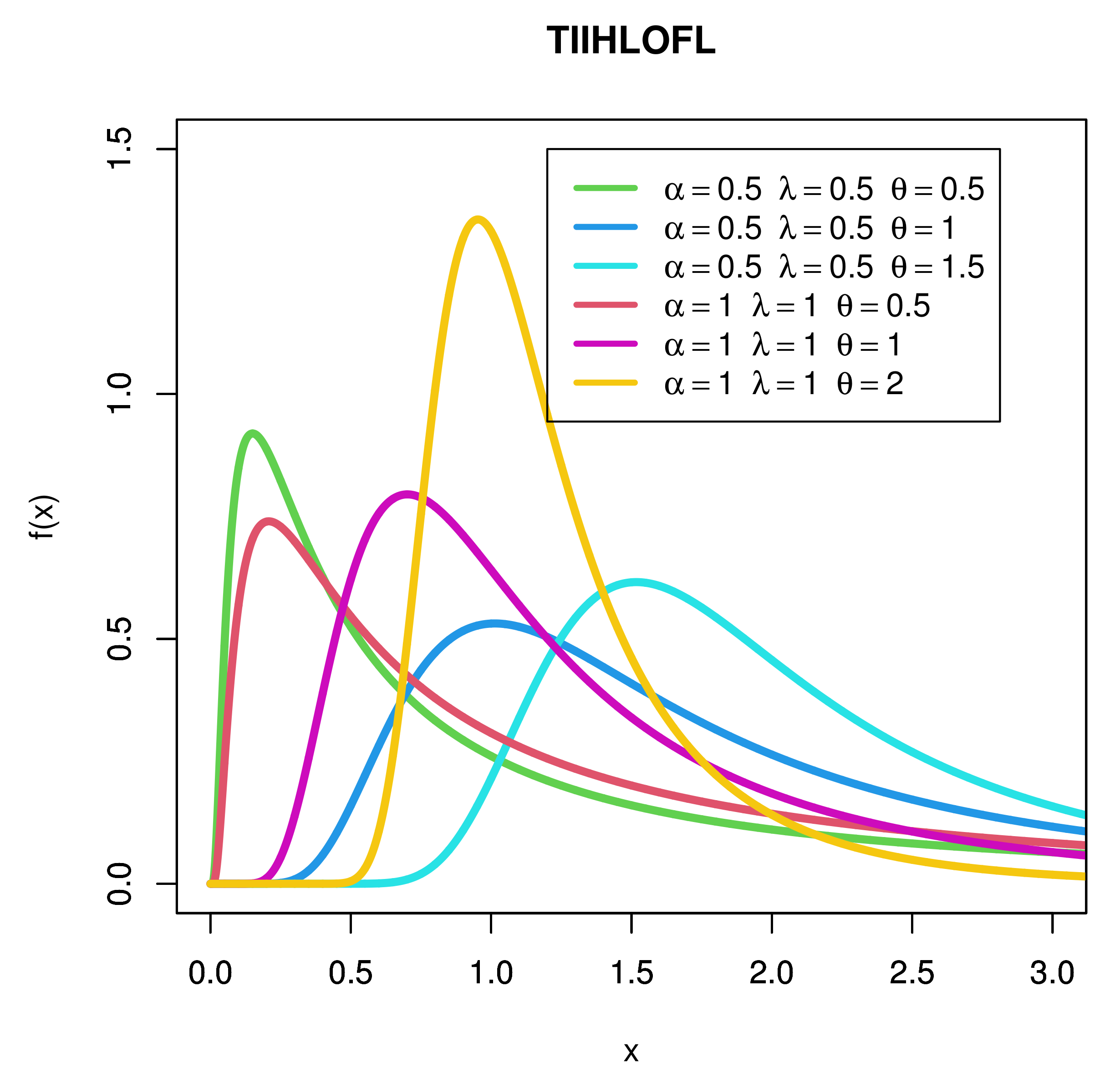
3.4. Type II Half-Logistic Odd Fréchet Lindely (TIIHLOFL) Distribution

Let Lindely be the baseline distribution having cdf and pdf $G(x;\phi )=1-(1+\frac{\lambda }{\lambda +1}x)e^{-\lambda x}$ and $g(x;\phi )=\frac{{\lambda }^2}{\lambda +1}(x+1)e^{-\lambda x}.$ The cdf and pdf of $TIIHLOFL$ model are provided below

$$F\left(x\right)=\frac{2e^{-\alpha {\left(\frac{(1+\frac{\lambda }{\lambda +1}x)e^{-\lambda x}}{1-(1+\frac{\lambda }{\lambda +1}x)e^{-\lambda x}}\right)}^{\theta }}}{1+e^{-\alpha {\left(\frac{(1+\frac{\lambda }{\lambda +1}x)e^{-\lambda x}}{1-(1+\frac{\lambda }{\lambda +1}x)e^{-\lambda x}}\right)}^{\theta }}},x>0,$$

and

$$f\left(x\right)=\frac{2\alpha \theta {\lambda }^2(x+1)e^{-\lambda x}{\left((1+\frac{\lambda }{\lambda +1}x)e^{-\lambda x}\right)}^{\theta -1}{e}^{-\alpha {\left(\frac{(1+\frac{\lambda }{\lambda +1}x)e^{-\lambda x}}{1-(1+\frac{\lambda }{\lambda +1}x)e^{-\lambda x}}\right)}^{\theta }}}{(\lambda +1){(1-(1+\frac{\lambda }{\lambda +1}x)e^{-\lambda x})}^{\theta +1}{\left[1+e^{-\alpha {\left(\frac{(1+\frac{\lambda }{\lambda +1}x)e^{-\lambda x}}{1-(1+\frac{\lambda }{\lambda +1}x)e^{-\lambda x}}\right)}^{\theta }}\right]}^2}.$$

Figure 4 describes the different forms of the pdf of TIIHLOFL distribution.

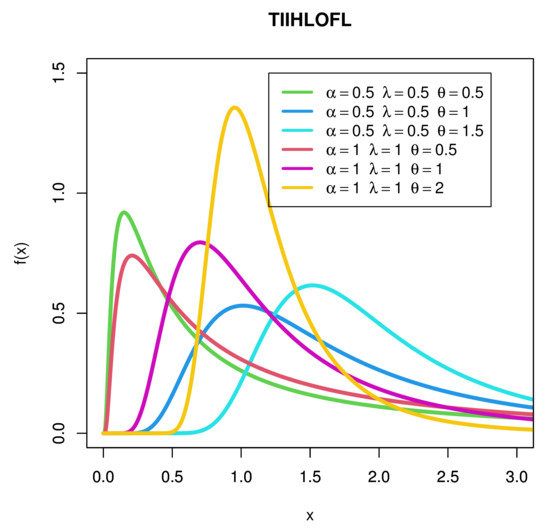
Figure 4. Shapes of the pdf of TIIHLOFL $(\alpha ,\lambda ,\theta )$ for various values of parameter.

4. Statistical Properties

In this section, we derive some statistical features for the $TIIHLOF-G$ class including ORMs, INMs, MGEF, REL, and RREL functions, and RéE.

4.1. Different Types of Moments

The rth ORM of the $TIIHLOF-G$ is

$${\mu }_r^{{}^{/}}=E\left(X^r\right)=\sum _{d=0}^{\infty }{\varpi }_{d}E\left(Z_{(d+1)}^r\right).$$

(16)

Table 1, Table 2 and Table 3 show the numerical values of $E\left(X\right)$, $E\left(X^2\right)$, $E\left(X^3\right)$, $E\left(X^4\right)$, Var(X), SK, KU, and coefficient of variation (CV) of the $TIIHLOFExp$ and $TIIHLOFR$ distributions.

Table 1. Numerical values of $E\left(X\right)$, $E\left(X^2\right)$, $E\left(X^3\right)$, $E\left(X^4\right)$, Var(X), SK, KU, and CV of the $TIIHLOFExp$ distribution.

$\mathit{\alpha }$	$\mathit{\lambda }$	$\mathit{\theta }$	$\mathit{E}\left(\mathit{X}\right)$	$\mathit{E}\left({\mathit{X}}^2\right)$	$\mathit{E}\left({\mathit{X}}^3\right)$	$\mathit{E}\left({\mathit{X}}^4\right)$	Var(X)	SK	KU	CV
0.5	0.5	0.5	1.386	8.647	98.110	1546.203	6.726	3.868	3.868	1.871
		0.9	1.183	3.394	18.738	154.587	1.994	3.552	3.552	1.193
		1.5	1.177	2.068	5.795	24.788	0.684	3.099	3.099	0.703
	0.9	0.5	0.770	2.669	16.823	147.291	2.076	3.868	3.868	1.871
		0.9	0.657	1.048	3.213	14.726	0.616	3.552	3.552	1.193
		1.5	0.654	0.638	0.994	2.361	0.211	3.099	3.099	0.703
	1.5	0.5	0.462	0.961	3.634	19.089	0.747	3.868	3.868	1.871
		0.9	0.394	0.377	0.694	1.908	0.222	3.552	3.552	1.193
		1.5	0.392	0.230	0.215	0.306	0.076	3.100	3.100	0.703
0.9	0.5	0.5	2.286	15.368	176.118	2781.125	10.144	2.929	2.929	1.393
		0.9	1.736	5.827	33.439	277.737	2.813	2.872	2.872	0.966
		1.5	1.531	3.239	9.975	44.119	0.894	2.693	2.693	0.617
	0.9	0.5	1.270	4.743	30.199	264.930	3.131	2.929	2.929	1.393
		0.9	0.964	1.798	5.730	26.457	0.868	2.868	2.868	0.966
		1.5	0.851	1.000	1.710	4.203	0.276	2.693	2.693	0.617
	1.5	0.5	0.762	1.708	6.523	34.335	1.127	2.929	2.929	1.393
		0.9	0.579	0.647	1.238	3.429	0.313	2.868	2.868	0.966
		1.5	0.510	0.360	0.369	0.545	0.099	2.693	2.693	0.617
1.5	0.5	0.5	3.395	24.984	291.692	4626.890	13.460	2.339	2.339	1.081
		0.9	2.351	9.119	54.810	461.069	3.590	2.424	2.424	0.806
		1.5	1.895	4.683	15.753	72.331	1.091	2.408	2.408	0.551
	0.9	0.5	1.886	7.711	50.016	440.757	4.154	2.339	2.339	1.081
		0.9	1.306	2.814	9.398	43.921	1.108	2.424	2.424	0.806
		1.5	1.053	1.445	2.701	6.890	0.337	2.408	2.408	0.551
	1.5	0.5	1.132	2.776	10.803	57.122	1.496	2.339	2.339	1.081
		0.9	0.784	1.013	2.030	5.692	0.399	2.424	2.424	0.806
		1.5	0.632	0.520	0.583	0.893	0.121	2.408	2.408	0.551

Table 2. Numerical values of $E\left(X\right)$, $E\left(X^2\right)$, $E\left(X^3\right)$, $E\left(X^4\right)$, Var(X), SK, KU, and CV of the $TIIHLOFR$ distribution.

$\mathit{\alpha }$	$\mathit{\lambda }$	$\mathit{\theta }$	$\mathit{E}\left(\mathit{X}\right)$	$\mathit{E}\left({\mathit{X}}^2\right)$	$\mathit{E}\left({\mathit{X}}^3\right)$	$\mathit{E}\left({\mathit{X}}^4\right)$	Var(X)	SK	KU	CV
0.5	0.5	0.5	1.260	2.772	8.786	34.588	1.184	1.793	1.793	0.863
		0.9	1.374	2.367	5.122	13.578	0.478	1.684	1.684	0.503
		1.5	1.469	2.353	4.170	8.274	0.195	1.629	1.629	0.300
	0.9	0.5	0.939	1.540	3.638	10.675	0.658	1.793	1.793	0.863
		0.9	1.024	1.315	2.121	4.191	0.266	1.684	1.684	0.503
		1.5	1.095	1.307	1.727	2.554	0.108	1.629	1.629	0.300
	1.5	0.5	0.728	0.924	1.691	3.843	0.395	1.793	1.793	0.863
		0.9	0.793	0.789	0.986	1.509	0.159	1.684	1.684	0.503
		1.5	0.848	0.784	0.803	0.919	0.065	1.629	1.629	0.300
0.9	0.5	0.5	1.777	4.571	15.319	61.470	1.412	1.295	1.295	0.669
		0.9	1.714	3.472	8.322	23.309	0.534	1.384	1.384	0.426
		1.5	1.689	3.063	6.023	12.957	0.210	1.463	1.463	0.271
	0.9	0.5	1.325	2.540	6.343	18.972	0.785	1.295	1.295	0.669
		0.9	1.278	1.929	3.446	7.194	0.297	1.384	1.384	0.426
		1.5	1.259	1.702	2.494	3.999	0.117	1.463	1.463	0.271
	1.5	0.5	1.026	1.524	2.948	6.830	0.471	1.295	1.295	0.669
		0.9	0.990	1.157	1.602	2.590	0.178	1.384	1.384	0.426
		1.5	0.975	1.021	1.159	1.440	0.070	1.463	1.463	0.271
1.5	0.5	0.5	2.304	6.789	24.223	99.935	1.483	0.970	0.970	0.529
		0.9	2.036	4.702	12.327	36.474	0.555	1.180	1.180	0.366
		1.5	1.890	3.790	8.124	18.731	0.218	1.343	1.343	0.247
	0.9	0.5	1.717	3.772	10.030	30.844	0.824	0.970	0.970	0.529
		0.9	1.518	2.612	5.104	11.257	0.309	1.180	1.180	0.366
		1.5	1.409	2.106	3.364	5.781	0.121	1.343	1.343	0.247
	1.5	0.5	1.330	2.263	4.662	11.104	0.494	0.970	0.970	0.529
		0.9	1.176	1.567	2.372	4.053	0.185	1.180	1.180	0.366
		1.5	1.091	1.263	1.563	2.081	0.073	1.343	1.343	0.247

Table 3. Numerical values of $E\left(X\right)$, $E\left(X^2\right)$, $E\left(X^3\right)$, $E\left(X^4\right)$, Var(X), SK, KU, and CV of the $TIIHLOFL$ distribution.

$\mathit{\alpha }$	$\mathit{\lambda }$	$\mathit{\theta }$	$\mathit{E}\left(\mathit{X}\right)$	$\mathit{E}\left({\mathit{X}}^2\right)$	$\mathit{E}\left({\mathit{X}}^3\right)$	$\mathit{E}\left({\mathit{X}}^4\right)$	Var(X)	SK	KU	CV
0.5	0.5	0.5	2.260	16.846	217.906	3836.068	11.740	3.152	3.152	1.516
		0.9	2.167	8.636	57.738	554.210	3.940	2.806	2.806	0.916
		1.5	2.256	6.553	25.753	138.065	1.463	2.469	2.469	0.536
	0.9	0.5	1.146	4.735	33.986	331.428	3.422	3.273	3.273	1.614
		0.9	1.068	2.276	8.404	44.729	1.135	2.935	2.935	0.997
		1.5	1.102	1.634	3.424	10.065	0.419	2.579	2.579	0.587
	1.5	0.5	0.633	1.550	6.632	38.591	1.150	3.405	3.405	1.695
		0.9	0.574	0.703	1.536	4.867	0.373	3.086	3.086	1.065
		1.5	0.586	0.479	0.576	0.997	0.136	2.719	2.719	0.630
0.9	0.5	0.5	3.595	29.612	390.003	6893.547	16.687	2.399	2.399	1.136
		0.9	3.022	14.300	101.607	991.829	5.165	2.314	2.314	0.752
		1.5	2.810	9.681	42.469	240.672	1.785	2.195	2.195	0.475
	0.9	0.5	1.849	8.356	60.885	595.744	4.938	2.476	2.476	1.202
		0.9	1.518	3.820	14.865	80.168	1.514	2.397	2.397	0.810
		1.5	1.395	2.466	5.738	17.692	0.519	2.272	2.272	0.516
	1.5	0.5	1.030	2.742	11.889	69.381	1.682	2.568	2.568	1.260
		0.9	0.826	1.190	2.726	8.731	0.507	2.502	2.502	0.862
		1.5	0.750	0.734	0.976	1.761	0.172	2.373	2.373	0.552
1.5	0.5	0.5	5.147	47.337	642.109	11444.724	20.848	1.932	1.932	0.887
		0.9	3.920	21.553	163.639	1635.462	6.187	1.991	1.991	0.635
		1.5	3.353	13.303	64.309	385.166	2.058	2.000	2.000	0.428
	0.9	0.5	2.680	13.430	100.417	989.623	6.248	1.981	1.981	0.933
		0.9	1.998	5.830	24.091	132.505	1.837	2.047	2.047	0.678
		1.5	1.685	3.446	8.815	28.564	0.605	2.057	2.057	0.462
	1.5	0.5	1.506	4.425	19.635	115.307	2.156	2.045	2.045	0.975
		0.9	1.100	1.834	4.438	14.455	0.624	2.123	2.123	0.718
		1.5	0.915	1.040	1.516	2.862	0.203	2.135	2.135	0.492

The sth INMs of the $TIIHLOF-G$ noted by ${\zeta }_s\left(t\right)$ for any real $s>0$, is

$${\zeta }_s\left(t\right)={\int }_{-\infty }^t{x}^{s}f\left(x\right)dx=\sum _{d=0}^{\infty }{\varpi }_d{\int }_{-\infty }^t{x}^s{h}_{(d+1)}\left(x\right)dx.$$

(17)

The MGEF of the $TIIHLOF-G$ is

$$M_X\left(t\right)=E\left(e^{tX}\right)=\sum _{d=0}^{\infty }{\varpi }_d{M}_{(d+1)}\left(t\right),$$

where $M_{(d+1)}\left(t\right)$ is the MGEF of $Z_{(d+1)}^{}$.

The rth-order moment of the REL of the $TIIHLOF-G$ is

$$\begin{array}{c}\hfill {\psi }_r\left(t\right)=\frac{1}{\overline{F}\left(t\right)}{\int }_t^{\infty }{(x-t)}^{r}f\left(x\right)dx,r\ge 1\\ & & \hfill \\ \hfill =\frac{1}{\overline{F}\left(t\right)}\sum _{d=0}^{\infty }{\varpi }_d^{*}{\int }_t^{\infty }{x}^r{h}_{(d+1)}\left(x\right)dx,\end{array}$$

(18)

where ${\varpi }_d^{*}={\displaystyle \sum _{d=0}^{\infty }}{\varpi }_d$${\sum }_{m=0}^r\left(\genfrac{}{}{0pt}{}{r}{m}\right){(-t)}^{r-m}.$ The rth-order moment of the RREL of the $TIIHLOF-G$ is

$$\begin{array}{c}\hfill m_r\left(t\right)=\frac{1}{F\left(t\right)}{\int }_0^t{(t-x)}^{r}f\left(x\right)dx,r\ge 1\\ & & \hfill \\ \hfill =\frac{1}{F\left(t\right)}\sum _{d=0}^{\infty }{\varpi }_d^{*}{\int }_0^t{x}^r{h}_{(d+1)}\left(x\right)dx,\end{array}$$

(19)

4.2. Rényi Entropy

The RéE of the $TIIHLOF-G$ is given below

$$I_R\left(\rho \right)=\frac{1}{1-\rho }log\left[{\int }_{-\infty }^{\infty }f{}^{\rho }\left(x\right)dx\right],\rho >0,\rho \ne 1.$$

(20)

Employing Equation (9) and the same manner of the beneficial expansion of Equation (15), we obtain, after a little simplification,

$$f^{\rho }\left(x\right)=\sum _{d=0}^{\infty }{\eta }_{d}g{\left(x\right)}^{\rho }G{\left(x\right)}^d,$$

where

$${\eta }_d=\sum _{i,k,m=0}^{\infty }\frac{{(-1)}^{k+m+d}{\left(\alpha i+\rho \right)}^k}{k!}\left(\genfrac{}{}{0pt}{}{-2\rho }{i}\right)\left(\genfrac{}{}{0pt}{}{-\theta (\rho +k)-\rho }{m}\right)\left(\genfrac{}{}{0pt}{}{\theta (\rho +k)+m-\rho }{d}\right).$$

Thus the RéE of $TIIHLOF-G$ class is given below

$$I_R\left(\rho \right)=\frac{1}{1-\rho }log\left\{\sum _{d=0}^{\infty }{\eta }_d{\int }_{-\infty }^{\infty }g{\left(x\right)}^{\rho }G{\left(x\right)}^{d}dx\right\}.$$

(21)

5. Estimation Methods

To evaluate the estimation problem of the $TIIHLOF-G$ family parameters, this part uses six estimate methods: maximum likelihood, least-square, a maximum product of spacing, weighted least square, Cramér-von Mises, and Anderson–Darling. For more examples see [29,30,31,32,33].

5.1. Method of Maximum Likelihood Estimation

Suppose $x_1,\cdots ,x_n$ represent a random sample of size n from the $TIIHLOF-G$ class having parameters $\alpha ,\theta$ and $\phi$. Consider $\Psi =$${(\alpha ,\theta ,\phi )}^T$ be a $p\times 1$ parameter vector. The log-likelihood (LL) function is defined as follows:

$$\begin{array}{ccc}\hfill L_n& =& nlog\left(2\alpha \right)+nlog\left(\theta \right)+\sum _{i=1}^{n}logg(x_i;\phi )+(\theta -1)\sum _{i=1}^{n}log\overline{G}(x_i;\phi )\hfill \\ & & -(\theta +1)\sum _{i=1}^{n}log\left(G(x_i;\phi )\right)-\alpha \sum _{i=1}^n{d}_i^{\theta }\hfill \\ & & -2\sum _{i=1}^{n}log\left\{1+e^{-\alpha d_i^{\theta }}\right\},\hfill \end{array}$$

(22)

where $d_i=\frac{\overline{G}(x_i;\phi )}{G(x_i;\phi )}.$ The components of score vector $U_n(\Psi )=\frac{\partial L_n}{\partial \Psi }=\left(\frac{\partial L_n}{\partial \alpha },\frac{\partial L_n}{\partial \theta },\frac{\partial L_n}{\partial {\phi }_k}\right)$ are given below

$$U_{\alpha }=\frac{\partial L_n}{\partial \alpha }=\frac{n}{\alpha }-\sum _{i=1}^n{d}_i^{\theta }+2\sum _{i=1}^n\frac{d_i^{\theta }{e}^{-\alpha d_i^{\theta }}}{1+e^{-\alpha d_i^{\theta }}},$$

(23)

$$\begin{array}{c}\hfill \begin{array}{ccc}{U}_{\theta }& =\hfill & \frac{\partial L_n}{\partial \theta }=\frac{n}{\theta }+\sum _{i=1}^{n}log\overline{G}(x_i;\phi )-\sum _{i=1}^{n}log\left(G(x_i;\phi )\right)\hfill \\ & & \\ & & -\alpha \sum _{i=1}^n{d}_i^{\theta }log\left(d_i\right)+2\sum _{i=1}^n\frac{\alpha d_i^{\theta }log\left(d_i\right)e^{-\alpha d_i^{\theta }}}{1+e^{-\alpha d_i^{theta}}},\hfill \end{array}\end{array}$$

(24)

and

$$\begin{array}{c}\hfill \begin{array}{ccc}{U}_{{\phi }_k}& =\hfill & \frac{\partial L_n}{\partial {\phi }_k}=\sum _{i=1}^n\frac{g^{\prime }(x_i;\phi )}{g(x_i;\phi )}+(\theta -1)\sum _{i=1}^n\frac{G^{\prime }(x_i;\phi )}{G(x_i;\phi )}-(\theta +1)\sum _{i=1}^n\frac{{\overline{G}}^{\prime }(x_i;\phi )}{\overline{G}(x_i;\phi )}\hfill \\ & & \\ & & -\alpha \theta \sum _{i=1}^n{d}_i^{\theta -1}\partial d_i\partial {\phi }_k-2\sum _{i=1}^n\frac{\alpha \theta d_i^{\theta -1}{e}^{-\alpha d_i^{\theta }}}{1+e^{-\alpha d_i^{\theta }}}\partial d_i\partial {\phi }_k,\hfill \end{array}\end{array}$$

(25)

where $g^{\prime }(x_i;\phi )=\frac{\partial g(x_i;\phi )}{\partial {\phi }_k},G^{\prime }(x_i;\phi )=\frac{\partial G(x_i;\phi )}{\partial {\phi }_k},{\overline{G}}^{\prime }(x_i;\phi )=\frac{\partial \overline{G}(x_i;\phi )}{\partial {\phi }_k}$.

5.2. Ordinary Least Squares and Weighted Least Squares Methods

The methods of ordinary least squares (OLS) and weighted least squares (WLS) are used to estimate the parameters of diverse distributions. Let $x_{\left(1\right)}<\cdots <x_{\left(n\right)}$ be a random sample with the $\Psi =$${(\alpha ,\theta ,\phi )}^T$ parameters from the $TIIHLOF-G$ class having parameters. OLS estimators (OLSE) and WLS estimators (WLSE) of the $\Psi =$${(\alpha ,\theta ,\phi )}^T$ distribution parameters of $TIIHLOF-G$ can be obtained by minimizing the following:

$$\begin{array}{c}\hfill V(\Psi )=\sum _{i=1}^n{\upsilon }_i{\left[\frac{2e^{-\alpha {\left(\frac{\overline{G}(x_{\left(i\right)},\phi )}{G(x_{\left(i\right)},\phi )}\right)}^{\theta }}}{1+e^{-\alpha {\left(\frac{\overline{G}(x_{\left(i\right)},\phi )}{G(x_{\left(i\right)},\phi )}\right)}^{\theta }}}\right]}^2\end{array}$$

(26)

${\upsilon }_i=1$ for OLSE and ${\upsilon }_i=\frac{{(n+1)}^2(n+2)}{\left[i\right(n-I+1\left)\right]}$ for WLSE with respect to $\alpha ,\theta ,$ and $\phi$. Furthermore, by resolving the nonlinear equations, the OLSE and WLSE with respect to $\alpha ,\theta ,$ and $\phi$.

5.3. Maximum Product of Spacings Method

If $x_{\left(1\right)}<\cdots <x_{\left(n\right)}$ is a random sample of the size n, you can describe the uniform spacing of the $TIIHLOF-G$ family as:

$$\begin{array}{c}\hfill D_i(\Psi )=F(x_{\left(i\right)},\Psi )-F(x_{(i-1)},\Psi );i=1,\cdots ,n+1\end{array}$$

(27)

where $D_i(\Psi )$ denotes to the uniform spacings, $F(x_{\left(0\right)},\Psi )=0$, $F(x_{(n+1)},\Psi )=1$ and ${\sum }_{i=1}^{n+1}{D}_i(\Psi )=1$. The maximum product of spacing (MPS) estimators (MPSE) of the $TIIHLOF-G$ family parameters can be obtained by maximizing

$$\begin{array}{c}\hfill G(\Psi )=\frac{1}{n+1}\sum _{i=1}^{n+1}ln\left\{{\left[\frac{2e^{-\alpha {\left(\frac{\overline{G}(x_{\left(i\right)},\phi )}{G(x_{\left(i\right)},\phi )}\right)}^{\theta }}}{1+e^{-\alpha {\left(\frac{\overline{G}(x_{\left(i\right)},\phi )}{G(x_{\left(i\right)},\phi )}\right)}^{\theta }}}\right]}^2-{\left[\frac{2e^{-\alpha {\left(\frac{\overline{G}(x_{(i-1)},\phi )}{G(x_{(i-1)},\phi )}\right)}^{\theta }}}{1+e^{-\alpha {\left(\frac{\overline{G}(x_{(i-1)},\phi )}{G(x_{(i-1)},\phi )}\right)}^{\theta }}}\right]}^2\right\}\end{array}$$

(28)

with respect to $\alpha ,\theta ,$ and $\phi$. Further, the MPSE of the $TIIHLOF-G$ family can also be obtained by solving nonlinear equation of derivatives of $G(\Psi )$ with respect to $\alpha ,\theta ,$ and $\phi$.

5.4. Cramér-von-Mises Method

In Cramér–von-Mises (CVM), we obtain the $TIIHLOF-G$ family by minimizing the following function with respect to $\alpha ,\theta ,$ and $\phi$; the CVM estimators (CVME) of the $TIIHLOF-G$ family parameters $\alpha ,\theta ,$ and $\phi$ are obtained.

$$\begin{array}{c}\hfill C(\Psi )=\frac{1}{12}+\sum _{i=1}^n{\left({\left[\frac{2e^{-\alpha {\left(\frac{\overline{G}(x_{\left(i\right)},\phi )}{G(x_{\left(i\right)},\phi )}\right)}^{\theta }}}{1+e^{-\alpha {\left(\frac{\overline{G}(x_{\left(i\right)},\phi )}{G(x_{\left(i\right)},\phi )}\right)}^{\theta }}}\right]}^2-\frac{2i-1}{2n}\right)}^2\end{array}$$

(29)

In addition, we resolve the nonlinear equations of derivatives of $C(\Psi )$ with respect to $\alpha ,\theta ,$ and $\phi$.

5.5. Anderson-Darling Method

In Anderson–Darling (AD), other forms of minimum distance estimators are the AD estimators (ADE). The ADE of the parameters of the $TIIHLOF-G$ family is acquired by minimizing

$$\begin{array}{c}\hfill A(\Psi )=-n-\frac{1}{n}\sum _{i=1}^n(2i-1){\left(ln\left({\left[\frac{2e^{-\alpha {\left(\frac{\overline{G}(x_{\left(i\right)},\phi )}{G(x_{\left(i\right)},\phi )}\right)}^{\theta }}}{1+e^{-\alpha {\left(\frac{\overline{G}(x_{\left(i\right)},\phi )}{G(x_{\left(i\right)},\phi )}\right)}^{\theta }}}\right]}^2\right)-ln\left(1-{\left[\frac{2e^{-\alpha {\left(\frac{\overline{G}(x_{(n+1-i)},\phi )}{G(x_{(n+1-i)},\phi )}\right)}^{\theta }}}{1+e^{-\alpha {\left(\frac{\overline{G}(x_{(n+1-i)},\phi )}{G(x_{(n+1-i)},\phi )}\right)}^{\theta }}}\right]}^2\right)\right)}^2\end{array}$$

(30)

for $\alpha ,\theta ,$ and $\phi$, respectively. It is also possible to obtain the ADE by resolving the nonlinear equations of derivatives of $A(\Psi )$ with respect to $\alpha ,\theta ,$ and $\phi$.

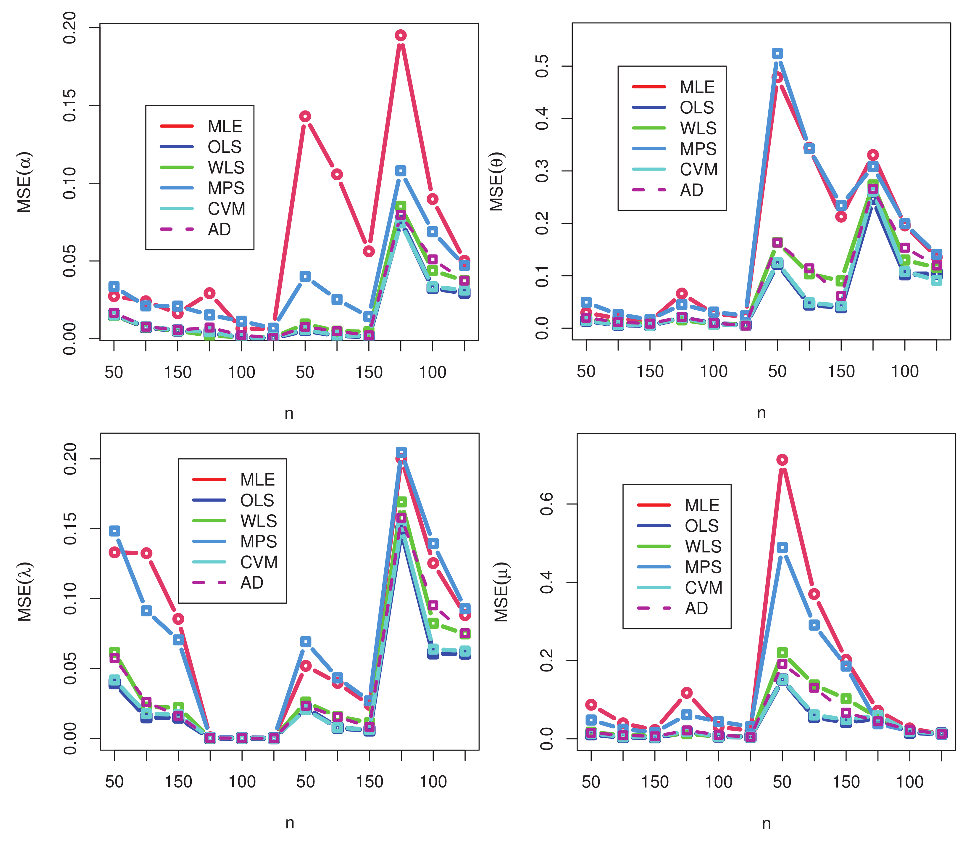
6. Numerical Outcomes

In this section, Monte Carlo simulations are run to evaluate the correctness and consistency of the new class’s six estimation methods. For the sake of example, the simulations are run with the estimators of the $TIIHLOFW$ distribution’s parameters. The simulation replication is taken as $N=1000$ and samples of sizes $n=50,100$ and 150 are generated by using the inverse transformation,

$$x_i=\frac{1}{\lambda }{\left[-log\left(1-\frac{1}{1+{[-\frac{1}{\alpha }log\left(\frac{U}{2-U}\right)]}^{\frac{1}{\theta }}}\right)\right]}^{\frac{1}{\mu }},i=1,2,\cdots ,n,$$

(31)

where U is a uniform distribution on $(0,1).$ The numerical outcomes are evaluated depending on the estimated relative biases (RB) and mean square errors (MSE). Table 4, shows the estimated RB and the MSE for the estimators of the parameters. Set four arbitrarily true values of ($\alpha ,\theta ,\lambda$ and $\mu$) such as Case I: ($\alpha =0.5;\theta =0.5;\lambda =0.5;\mu =0.5$), Case II: ($\alpha =1.5;\theta =1.5;\lambda =0.5;\mu =2$), Case III: ($\alpha =3;\theta =1.5;\lambda =3;\mu =2$), and Case IV: ($\alpha =3;\theta =1.5;\lambda =3;\mu =0.5$).

Table 4. The MLE, OLS, WLS, MPS, CVM, and AD estimated RB and MSE of the $TIIHLOFW$ distribution.

			MLE		OLS		WLS		MPS		CVM		AD
Case	n		RB	MSE	RB	MSE	RB	MSE	RB	MSE	RB	MSE	RB	MSE
I	50	$\alpha$	0.0900	0.0274	0.0289	0.0154	0.0296	0.0150	0.0897	0.0335	0.0039	0.0153	0.0280	0.0167
		$\theta$	0.0823	0.0296	0.0120	0.0142	0.0355	0.0188	0.0826	0.0494	−0.0043	0.0142	0.0364	0.0201
		$\lambda$	0.1366	0.1331	0.0488	0.0395	0.0545	0.0615	0.1357	0.1484	0.0801	0.0418	0.0875	0.0574
		$\mu$	0.0280	0.0870	0.0247	0.0115	0.0209	0.0169	0.0278	0.0480	0.0777	0.0139	0.0279	0.0155
	100	$\alpha$	0.0686	0.0241	0.0104	0.0074	0.0062	0.0076	0.0687	0.0211	−0.0024	0.0078	0.0118	0.0078
		$\theta$	0.0648	0.0183	0.0077	0.0066	0.0263	0.0105	0.0651	0.0262	0.0015	0.0066	0.0301	0.0115
		$\lambda$	0.1086	0.1325	0.0091	0.0151	0.0038	0.0224	0.1084	0.0913	0.0240	0.0177	0.0340	0.0260
		$\mu$	−0.0169	0.0395	0.0067	0.0046	0.0065	0.0091	−0.0171	0.0247	0.0302	0.0051	0.0066	0.0090
	150	$\alpha$	0.0496	0.0164	0.0059	0.0053	−0.0007	0.0051	0.0620	0.0210	0.0002	0.0054	0.0047	0.0056
		$\theta$	0.0425	0.0126	0.0058	0.0057	0.0174	0.0099	0.0429	0.0165	−0.0014	0.0056	0.0218	0.0088
		$\lambda$	0.0915	0.0855	0.0091	0.0149	0.0037	0.0221	0.0915	0.0705	0.0237	0.0169	0.0138	0.0162
		$\mu$	−0.0153	0.0225	0.0060	0.0039	0.0052	0.0081	−0.0163	0.0165	0.0301	0.0045	0.0062	0.0063
II	50	$\alpha$	0.0030	0.0293	0.0028	0.0037	0.0025	0.0021	0.0029	0.0153	0.0075	0.0045	0.0078	0.0072
		$\theta$	−0.0122	0.0660	−0.0082	0.0194	−0.0011	0.0158	−0.0123	0.0452	0.0075	0.0199	0.0009	0.0212
		$\lambda$	−0.0066	0.0008	−0.0022	0.0003	−0.0021	0.0003	−0.0067	0.0006	−0.0004	0.0003	−0.0008	0.0003
		$\mu$	−0.0178	0.1174	0.0009	0.0168	0.0027	0.0129	−0.0180	0.0614	0.0143	0.0191	0.0078	0.0214
	100	$\alpha$	−0.0024	0.0065	−0.0014	0.0007	0.0004	0.0010	−0.0025	0.0113	0.0014	0.0008	0.0015	0.0023
		$\theta$	0.0041	0.0277	−0.0062	0.0083	−0.0011	0.0071	0.0041	0.0307	0.0004	0.0077	−0.0008	0.0099
		$\lambda$	−0.0055	0.0003	−0.0002	0.0002	0.0005	0.0002	−0.0055	0.0004	0.0009	0.0002	0.0005	0.0002
		$\mu$	−0.0172	0.0301	−0.0004	0.0057	−0.0001	0.0057	−0.0172	0.0439	0.0032	0.0056	0.0006	0.0100
	150	$\alpha$	−0.0024	0.0064	−0.0012	0.0006	−0.0004	0.0009	−0.0024	0.0068	0.0004	0.0007	−0.0004	0.0006
		$\theta$	0.0040	0.0217	−0.0003	0.0062	0.0011	0.0070	0.0040	0.0241	0.0003	0.0057	0.0007	0.0049
		$\lambda$	−0.0053	0.0002	−0.0001	0.0001	−0.0003	0.0001	−0.0054	0.0003	0.0007	0.0001	0.0002	0.0001
		$\mu$	−0.0129	0.0211	−0.0004	0.0051	−0.0001	0.0057	−0.0149	0.0314	0.0013	0.0046	−0.0006	0.0040
III	50	$\alpha$	0.0201	0.1430	0.0056	0.0055	0.0078	0.0095	0.0200	0.0401	0.0082	0.0059	0.0087	0.0077
		$\theta$	0.1100	0.4787	−0.0042	0.1231	0.0105	0.1636	0.1107	0.5244	−0.0011	0.1252	0.0167	0.1633
		$\lambda$	−0.0090	0.0519	0.0037	0.0217	0.0014	0.0260	−0.0092	0.0692	0.0028	0.0205	−0.0002	0.0234
		$\mu$	−0.0111	0.7129	0.0298	0.1515	0.0330	0.2199	−0.0119	0.4888	0.0568	0.1518	0.0356	0.1916
	100	$\alpha$	0.0148	0.1057	0.0012	0.0021	0.0037	0.0049	0.0147	0.0253	0.0019	0.0022	0.0039	0.0048
		$\theta$	0.0977	0.3444	−0.0042	0.0452	0.0041	0.1036	0.0978	0.3428	0.0010	0.0485	0.0137	0.1142
		$\lambda$	−0.0081	0.0397	0.0033	0.0076	0.0013	0.0157	−0.0081	0.0433	0.0017	0.0077	0.0002	0.0153
		$\mu$	−0.0103	0.3699	0.0070	0.0559	0.0205	0.1377	−0.0113	0.2907	0.0159	0.0610	0.0175	0.1306
	150	$\alpha$	0.0107	0.0562	0.0002	0.0015	0.0033	0.0045	0.0108	0.0142	0.0010	0.0017	0.0014	0.0022
		$\theta$	0.0848	0.2128	0.0031	0.0400	0.0040	0.0902	0.0862	0.2343	0.0010	0.0428	0.0120	0.0615
		$\lambda$	−0.0080	0.0240	0.0001	0.0057	−0.0009	0.0113	−0.0081	0.0269	−0.0005	0.0063	−0.0002	0.0083
		$\mu$	−0.0106	0.2019	−0.0014	0.0433	0.0038	0.1024	−0.0106	0.1858	0.0072	0.0486	0.0012	0.0668
IV	50	$\alpha$	0.0062	0.1951	−0.0112	0.0759	−0.0106	0.0852	0.0064	0.1080	−0.0140	0.0745	−0.0064	0.0797
		$\theta$	0.0272	0.3304	−0.0230	0.2467	−0.0230	0.2735	0.0274	0.3084	−0.0362	0.2605	−0.0200	0.2659
		$\lambda$	−0.0129	0.2002	0.0064	0.1492	0.0059	0.1692	−0.0131	0.2047	0.0091	0.1519	0.0050	0.1579
		$\mu$	0.0509	0.0720	0.1289	0.0521	0.1382	0.0543	0.0502	0.0384	0.1805	0.0601	0.1350	0.0447
	100	$\alpha$	0.0062	0.0898	−0.0044	0.0327	−0.0073	0.0439	0.0057	0.0688	−0.0077	0.0334	−0.0059	0.0510
		$\theta$	0.0261	0.1960	0.0069	0.1027	−0.0064	0.1301	0.0237	0.1994	−0.0118	0.1083	−0.0132	0.1535
		$\lambda$	−0.0101	0.1254	0.0018	0.0608	0.0035	0.0824	−0.0102	0.1395	0.0057	0.0639	0.0047	0.0952
		$\mu$	0.0080	0.0266	0.0330	0.0159	0.0558	0.0202	0.0077	0.0199	0.0635	0.0191	0.0735	0.0223
	150	$\alpha$	0.0060	0.0501	−0.0027	0.0296	−0.0020	0.0373	0.0046	0.0471	−0.0032	0.0313	0.0007	0.0374
		$\theta$	0.0251	0.1355	0.0058	0.1032	0.0059	0.1154	0.0161	0.1409	0.0059	0.0911	0.0127	0.1197
		$\lambda$	−0.0093	0.0882	−0.0006	0.0607	−0.0017	0.0748	−0.0101	0.0928	−0.0006	0.0625	−0.0045	0.0752
		$\mu$	−0.0073	0.0126	0.0309	0.0138	0.0350	0.0136	−0.0069	0.0107	0.0440	0.0139	0.0300	0.0130

Extensive computations were carried out using the R statistical programming language software, with the most useful statistical package being the “stats” package, which used the conjugate-gradient maximization algorithm.

From Table 4, we are able to make the following observations. The performances of the proposed estimates of $\alpha ,\theta ,\lambda$, and $\mu$ in terms of their RB and MSE become better as n increases, as expected, where the results revealed that as the sample size increases, RB and MSE decrease. These findings clearly demonstrate the estimation methods estimators’ accuracy and consistency. As a result, the six estimation methods approach performs well in estimating the parameters of the $TIIHLOFW$ distribution. By the results of Table 4 and Figure 5, we show the OLS method and CVM method of estimation are better than other methods.

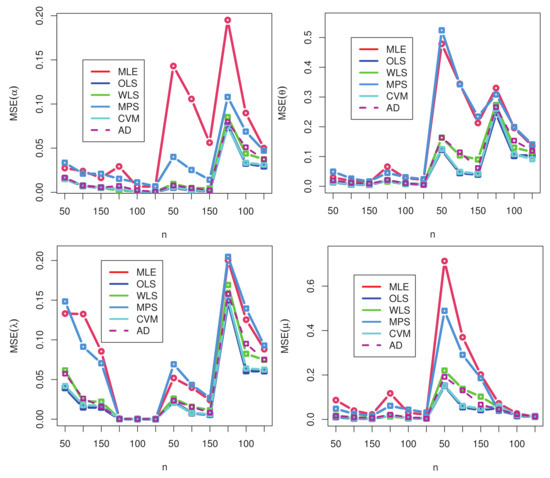
Figure 5. MSE with different sample sizes.

7. Applications

Here, we provide three applications to demonstrate the adaptability of the new recommended family. Some measures of goodness of fit are used to illustrate the flexibility of the TIIHLOF-G: the values of negative LL function (−LL), KAINC (Akaike Information Criterion (INC) ), KCAINC (Akaike INC with correction), KBINC (Bayesian INC), and KHQINC (Hannon–Quinn INC) are computed for all competitive models in order to verify which distribution fits the data more closely. The best distribution has the lowest numerical values of −LL, KAINC, KCAINC, KBINC, and KHQINC.

7.1. The Biomedical Data Set

The set of data just on relief times of 20 patients who received an analgesic (Gross and Clark, 1975) is 1.50, 1.20, 2.30, 1.80, 2.20, 1.70, 1.10, 4.10, 1.80, 1.60, 1.40, 1.40, 3.00, 1.70, 1.30, 1.60, 1.70, 1.90, 2.70, 2.00.

Throughout this subsection, we apply the TIIHLOFExp model to a real-world data set to assess its adaptability. To compare the TIIHLOFExp model to the other ten fitted distributions, one, two, three, four, and five parameters are employed. We compare the TIIHLOFExp distribution with the beta transmuted Weibull (BTW), Type I half-Logistic inverse power Ailamujia (TIHLIPA), McDonald log-logistic (McLL), Marshall–Olkin exponential (M-OExp), McDonald Weibull (McW), Burr X-Ex (BrXExp), transmuted exponentiated Chen (TEC), Kumaraswamy Ex (KwExp), generalized Marshall–Olkin Ex (GM-OExp), transmuted complementary Weibull-geometric (TCWG), beta Ex (BExp), Kumaraswamy Marshall–Olkin Ex (KwM-OExp), transmuted Chen (TC), Ailamujia (A), inverse Ailamujia (IA), Exp, beta Lomax (BL), gamma-Chen (GaC), Chen (C), Weibull Lomax (WL), Kumaraswamy Chen (KwC), odd log-logistic Weibull (OLL-W), beta Weibull (BW), beta-Chen (BC), Weibull (W), and Marshall–Olkin Chen (M-OC) models. All of these competitive models are mentioned in Al-Moisheer and Alotaibi (2022).

The parameter estimates and the numerical value of negative LL are presented in Table 5. Additionally, the numerical values of KAINC, KCAINC, KBINC, and KHQINC statistics for the biomedical data are presented in Table 6.

Table 5. The parameter estimates and the numerical values of −LL of the biomedical data.

Model	ML Estimates	−LL
TIIHLOFExp	$\widehat{\alpha }=0.052$, $\widehat{\lambda }=0.179$, $\widehat{\theta }=2.973$	15.392
BTW	$\widehat{\alpha }=5.619$, $\widehat{\beta }=0.531$, $\widehat{a}=53.344$, $\widehat{b}=3.568$, $\widehat{\lambda }=-0.772$	16.831
TIHLIPA	$\widehat{\alpha }=0.246$, $\widehat{\beta }=4.713$, $\widehat{\gamma }=-6.781$	16.095
McLL	$\widehat{\alpha }=0.881$, $\widehat{\beta }=2.070$, $\widehat{a}=19.225$, $\widehat{b}=32.033$, $\widehat{c}=1.926$	16.526
M-OExp	$\widehat{\alpha }=54.474$, $\widehat{\beta }=2.316$	19.755
McW	$\widehat{\alpha }=2.774$, $\widehat{\beta }=0.380$, $\widehat{a}=79.108$, $\widehat{b}=17.898$, $\widehat{c}=3.006$	16.927
BrXExp	$\widehat{\alpha }=1.164$, $\widehat{\beta }=0.321$	22.050
TEC	$\widehat{\alpha }=300.010$, $\widehat{\beta }=0.500$, $\widehat{a}=2.430$, $\widehat{b}=0.340$	15.780
KwExp	$\widehat{a}=83.756$, $\widehat{b}=0.568$, $\widehat{\beta }=3.333$	17.890
GM-OExp	$\widehat{\lambda }=0.519$, $\widehat{\alpha }=89.462$, $\widehat{\beta }=3.169$	18.375
TCWG	$\widehat{\alpha }=43.663$, $\widehat{\beta }=5.127$, $\widehat{\gamma }=0.282$, $\widehat{\lambda }=-0.271$	16.587
BExp	$\widehat{a}=81.633$, $\widehat{b}=0.542$, $\widehat{\beta }=3.514$	18.740
KwM-OExp	$\widehat{\alpha }=8.868$, $\widehat{\beta }=4.899$, $\widehat{a}=34.826$, $\widehat{b}=0.299$	17.400
TC	$\widehat{\alpha }=0.750$, $\widehat{a}=0.070$, $\widehat{b}=1.020$	23.815
A	$\widehat{\beta }=0.950$	26.160
IA	$\widehat{\beta }=3.449$	25.827
Exp	$\widehat{\beta }=0.526$	32.835
BL	$\widehat{a}=41.070$, $\widehat{b}=1.929$, $\widehat{\theta }=5.774$, $\widehat{\lambda }=0.429$	16.110
GaC	$\widehat{\alpha }=7.590$, $\widehat{\beta }=1.990$, $\widehat{a}=5.000$, $\widehat{b}=0.530$	23.175
C	$\widehat{a}=0.140$, $\widehat{b}=0.950$	24.570
WL	$\widehat{a}=14.739$, $\widehat{b}=5.585$, $\widehat{\theta }=0.263$, $\widehat{\lambda }=0.219$	19.631
KwC	$\widehat{\alpha }=160.070$, $\widehat{\beta }=0.490$, $\widehat{a}=2.210$, $\widehat{b}=0.520$	16.010
OLL-W	$\widehat{\alpha }=31.414$, $\widehat{\lambda }=0.134$, $\widehat{\theta }=26.771$	16.551
BW	$\widehat{\alpha }=0.831$, $\widehat{\beta }=0.613$, $\widehat{a}=29.947$, $\widehat{b}=11.632$	16.804
BC	$\widehat{\alpha }=85.870$, $\widehat{\beta }=0.480$, $\widehat{a}=2.010$, $\widehat{b}=0.55$	16.255
W	$\widehat{\lambda }=0.002$, $\widehat{\theta }=1.435$	20.586
M-OC	$\widehat{\alpha }=400.010$, $\widehat{a}=2.320$, $\widehat{b}=0.430$	19.440

Table 6. The numerical values of KAINC, KCAINC, KBINC, and KHQINC statistics for the biomedical data.

Models	KAINC	KCAINC	KBINC	KHQINC
TIIHLOFExp	36.784	38.284	34.688	37.368
BTW	43.662	50.124	39.468	44.828
TIHLIPA	38.189	39.112	36.092	38.772
McLL	43.051	47.337	39.556	44.023
M-OExp	43.51	45.51	44.22	43.9
McW	43.854	48.14	40.359	44.826
BrXExp	48.1	50.1	48.8	48.5
TEC	39.56	42.227	36.764	40.338
KwExp	41.78	44.75	43.28	42.32
GM-OExp	42.75	45.74	44.25	43.34
TCWG	51.173	55.459	47.678	52.145
BExp	43.48	46.45	44.98	44.02
KwM-OExp	42.8	46.84	45.55	43.6
TC	53.63	55.13	51.533	54.213
A	54.32	55.31	54.54	54.5
IA	53.653	53.888	52.954	53.847
Exp	67.67	68.67	67.89	67.87
BL	40.219	42.886	37.423	40.997
GaC	46.35	49.017	43.554	47.128
C	53.14	53.846	51.742	53.529
WL	47.261	49.928	44.465	48.039
KwC	40.02	42.687	37.224	40.798
OLL-W	39.101	40.601	37.004	39.684
BW	41.607	44.274	38.811	42.385
BC	40.51	43.177	37.714	41.288
W	45.1728	45.8786	45.5615	47.1642
M-OC	44.88	46.38	42.783	45.463

From Table 5 and Table 6, the values of −LL, KAINC, KCAINC, KBINC, and KHQINC are minimum for the $TIIHLOFExp$ distribution. Thus the $TIIHLOFExp$ distribution is a better model for the biomedical data as compared with the other twenty-six models.

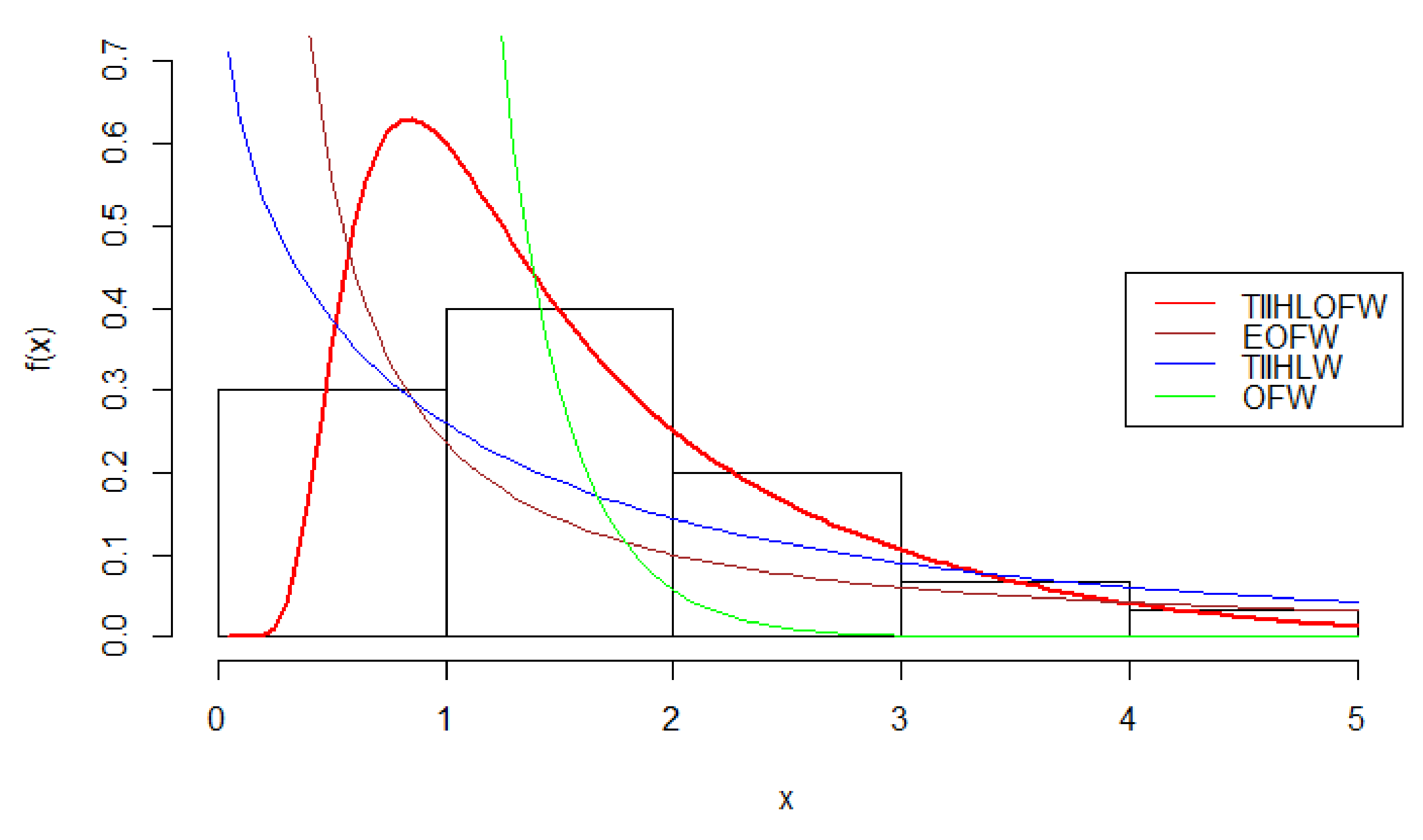
7.2. Engineering Data Set

The second data have been obtained from [34], it is for the time between failures (thousands of hours) of secondary reactor pumps. The data are as follows:

1.9210, 4.0820, 0.1990, 2.1600, 0.7460, 6.5600, 4.9920, 0.3470, 0.1500, 0.3580, 0.1010, 1.3590, 3.4650, 1.0600, 0.6140, 0.6050, 0.4020, 0.9540, 0.4910, 0.2730, 0.0700, 0.0620, 5.320.

We compare the fit of the $TIIHLOFW$ distribution with the following continuous lifetime distributions:

(i) Extended OF Weibull (EOFW) distribution of [12] has pdf given by

$$f(x;\lambda ,\alpha ,\mu ,\theta )=\frac{\alpha \theta \mu {\lambda }^{\mu }{x}^{\mu -1}{e}^{-{\left(\lambda x\right)}^{\mu }}{[1-{(1-e^{-{\left(\lambda x\right)}^{\mu }})}^{\alpha }]}^{\theta -1}}{{[1-e^{-{\left(\lambda x\right)}^{\mu }}]}^{\alpha \theta +1}},x>0.$$

(ii) Type II HL Weibull (TIIHLW) distribution of [28] has pdf given by

$$f(x;\lambda ,\alpha ,\mu ,\theta )=\frac{2\theta \mu {\lambda }^{\mu }{x}^{\mu -1}{e}^{-{\left(\lambda x\right)}^{\mu }}{(1-e^{-{\left(\lambda x\right)}^{\mu }})}^{\theta -1}}{{[1+{(1-e^{-{\left(\lambda x\right)}^{\mu }})}^{\theta }]}^2},x>0.$$

(iii) OF Weibull (OFW) distribution of [1] has pdf given by

$$f(x;\lambda ,\mu ,\theta )=\frac{\theta \mu {\lambda }^{\mu }{x}^{\mu -1}{e}^{-{\left(\lambda x\right)}^{\mu }}{\left(e^{-{\left(\lambda x\right)}^{\mu }}\right)}^{\theta -1}{e}^{-(\frac{e^{{-\left(\lambda x\right)}^{\mu }}}{1-e^{-{\left(\lambda x\right)}^{\mu }}}{)}^{\theta }}}{{(1-e^{-{\left(\lambda x\right)}^{\mu }})}^{\theta +1}},x>0.$$

The parameter estimates and the numerical value of negative LL are presented in Table 7. Additionally, the numerical values of KAINC, KCAINC, KBINC, and KHQINC statistics for the engineering data are presented in Table 8.

Table 7. The parameter estimates and the numerical values of −LL of the engineering data.

Model	ML Estimates	−LL
TIIHLOFW	$\widehat{\lambda }=0.3901$, $\widehat{\alpha }=0.5884$, $\widehat{\mu }=1.4299$, $\widehat{\theta }=0.3758$	30.759
EOFW	$\widehat{\lambda }=0.5436$, $\widehat{\alpha }=0.9057$, $\widehat{\mu }=0.3694$, $\widehat{\theta }=0.1980$	45.418
TIIHLW	$\widehat{\lambda }=0.3474$, $\widehat{\mu }=0.8837$, $\widehat{\theta }=0.9501$	32.574
OFW	$\widehat{\lambda }=0.0464$, $\widehat{\mu }=0.0575$, $\widehat{\theta }=0.7175$	60.544

Table 8. The numerical values of KAINC, KCAINC, KBINC, and KHQINC statistics for the engineering data.

Models	KAINC	KCAINC	KBINC	KHQINC
TIIHLOFW	69.519	71.741	74.061	70.661
EOFW	98.836	101.058	103.378	99.978
TIIHLW	71.147	72.410	74.554	72.004
OFW	127.087	128.350	130.494	127.944

From Table 7 and Table 8, the values of −LL, KAINC, KCAINC, KBINC, and KHQINC are minimum for the $TIIHLOFW$ distribution. Thus the $TIIHLOFW$ distribution is a better model for the engineering data as compared with the other three models. Figure 6 displays the fitted pdf plots of the engineering data set.

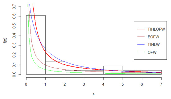
Figure 6. Fitted pdf for the engineering data set.

7.3. Environmental Data Set

The third data set is obtained from [35], it consists of thirty successive values of March precipitation (in inches) in Minneapolis/St Paul. The data are as follows:

1.180, 1.350, 4.750, 0.770, 1.950, 1.200, 0.470, 1.430, 3.370, 2.200, 3.000, 3.090, 1.510, 2.100, 0.520, 1.620, 1.310, 0.320, 0.590, 0.810, 2.810, 1.870, 2.480, 0.960, 1.890, 0.900, 1.740, 0.810, 1.200, 2.050.

We compare the fit of the $TIIHLOFW$ distribution with the following continuous lifetime distributions: EOFW, TIIHLW, and OFW models.

The parameter estimates and the numerical value of negative LL are presented in Table 9. Additionally, the numerical values of KAINC, KCAINC, KBINC, and KHQINC statistics for the environmental data are presented in Table 10.

Table 9. The parameter estimates and the numerical values of −LL of the environmental data.

Model	ML Estimates	−LL
TIIHLOFW	$\widehat{\lambda }=0.5477$, $\widehat{\alpha }=0.9205$, $\widehat{\mu }=1.8387$, $\widehat{\theta }=0.6241$	38.944
EOFW	$\widehat{\lambda }=0.2927$, $\widehat{\alpha }=0.8943$, $\widehat{\mu }=0.2182$, $\widehat{\theta }=1.0587$	55.876
TIIHLW	$\widehat{\lambda }=0.2675$, $\widehat{\mu }=0.9643$, $\widehat{\theta }=0.9297$	50.921
OFW	$\widehat{\lambda }=0.9615$, $\widehat{\mu }=1.5339$, $\widehat{\theta }=1.5469$	50.501

Table 10. The numerical values of KAINC, KCAINC, KBINC, and KHQINC statistics for the environmental data.

Models	KAINC	KCAINC	KBINC	KHQINC
TIIHLOFW	85.887	87.487	91.492	87.680
EOFW	119.752	121.352	125.357	121.545
TIIHLW	107.842	108.765	112.046	109.187
OFW	107.002	107.925	111.205	108.346

From Table 9 and Table 10, the values of −LL, KAINC, KCAINC, KBINC, and KHQINC are minimum for the $TIIHLOFW$ distribution. Thus the $TIIHLOFW$ distribution is a better model for the environmental data as compared with the other three models. Figure 7 displays the fitted pdf plots of the environmental data set.

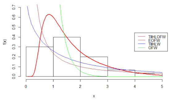
Figure 7. Fitted pdf for the environmental data.

7.4. Strength Data

The fourth data set is obtained from Ahmadini et al. [36], it consists of 56 values of strength data measured in GPA, the single carbon fibers, and 1000 impregnated carbon fiber tows. The data are as follows:

2.247, 2.64, 2.908, 3.099, 3.126, 3.245, 3.328, 3.355, 3.383, 3.572, 3.581, 3.681, 3.726, 3.727, 3.728, 3.783, 3.785, 3.786, 3.896, 3.912, 3.964, 4.05, 4.063, 4.082, 4.111, 4.118, 4.141, 4.246, 4.251, 4.262, 4.326, 4.402, 4.457, 4.466, 4.519, 4.542, 4.555, 4.614, 4.632, 4.634, 4.636, 4.678, 4.698, 4.738, 4.832, 4.924, 5.043, 5.099, 5.134, 5.359, 5.473, 5.571, 5.684, 5.721, 5.998, 6.06

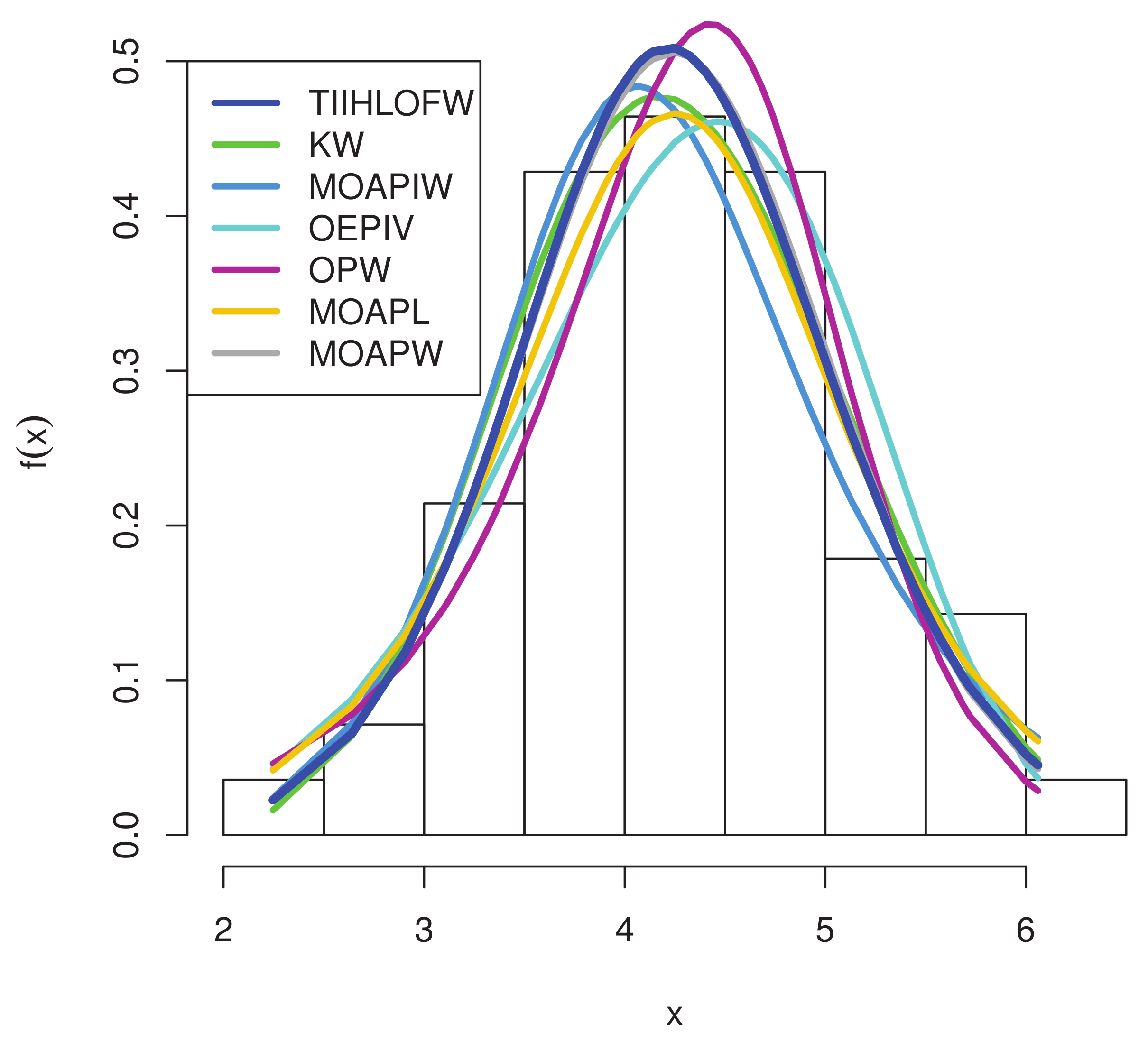
We compare the fit of the $TIIHLOFW$ distribution with the following continuous lifetime distributions: Kumaraswamy Weibull (KW) by Cordeiro et al. [37], Marshall–Olkin alpha power Weibull (MOAPW) by Almetwally [38], Marshall–Olkin alpha power inverse Weibull (MOAPIW) by Basheer et al. [32], odd Perks Weibull (OPW) by Elbatal et al. [14], Marshall–Olkin alpha power Lomax (MOAPL) by Almongy et al. [33], and Odds exponential-Pareto IV (OWPIV) by Baharith et al. [39].

The parameter estimates and the numerical value of negative LL are presented in Table 11. Additionally, the numerical values of KAINC, KCAINC, KBINC, and KHQINC statistics for the environmental data are presented in Table 12.

Table 11. The parameter estimates and the numerical values of −LL of the strength data.

Model	ML Estimates				−LL
TIIHLOFW	$\alpha =$ 5.2701,	0.3450	$\theta =$ 0.373,	$\mu =$ 3.2985,	67.7818
MOAPL	$\alpha =$ 281.8156,	$\beta =$ 270.1004,	$\theta =$ 550.4996,	$\lambda =$ 140.7209,	69.1317
MOAPW	$\alpha =$ 44.4414,	$\beta =$ 7.5156,	$\theta =$ 0.0101,	$\lambda =$ 5.7759,	67.9200
OPW	$\beta =$ 0.0101,	$\theta =$ 0.1355,	$\lambda =$ 0.3678,	$\delta =$ 0.5165,	70.2290
KW	$\alpha =$ 0.008,	$\beta =$ 4.1936,	$a=$ 2.8883,	$b=$ 0.2909,	67.9350
MOAPIW	$\alpha =$ 10.5695,	$\beta =$ 7.9752,	$\theta =$ 353.0412,	$\lambda =$ 100.1504,	69.3700
OEPIV	$\alpha =$ 40.7601,	$\beta =$ 0.1777,	$\theta =$ 54.1619,	$\lambda =$ 18.1516,	69.0468

Table 12. The numerical values of KAINC, KCAINC, KBINC, and KHQINC statistics for the strength data.

Model	KAINC	KCAINC	KBINC	KHQINC
TIIHLOFW	143.5636	144.3479	151.6650	146.7045
MOAPL	146.2634	147.0477	154.3648	149.4043
MOAPW	143.8401	144.6244	151.9415	146.9810
OPW	148.4581	149.2424	156.5595	151.5990
KW	143.8700	144.6543	151.9714	147.0109
MOAPIW	146.7408	147.5251	154.8422	149.8817
OEPIV	146.0936	146.8779	154.1950	149.2345

From Table 11 and Table 12, the values of −LL, KAINC, KCAINC, KBINC, and KHQINC are minimum for the $TIIHLOFW$ distribution. Thus the $TIIHLOFW$ distribution is a better model for the environmental data as compared with the other three models. Figure 8 displays the fitted pdf plots of the strength data set.

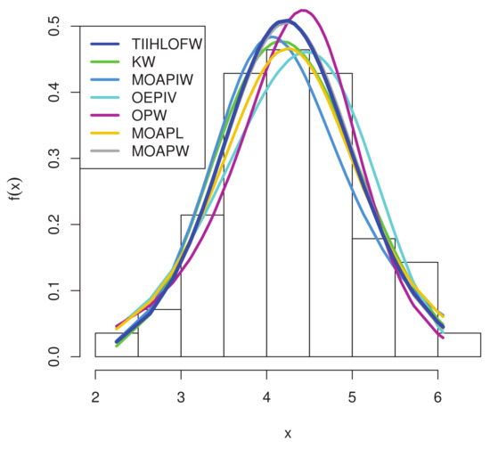
Figure 8. Fitted pdf for the strength data.

8. Conclusions and Summary

We presented a new class of continuous distributions entitled the Type II half-Logistic odd Fréchet-G class in this work. The identifiability of the proposed model was proved and also studied its relationship with other families of distributions. Some statistical properties such as ORMs, INMs, MGEF, REL, RREL, and entropy are derived. The estimates of the parameters of the new model are estimated using the ML method. A simulation outcome was conducted to check the performance of the MLE method. Using four real-life data sets we illustrated the flexibility of the TIIHLOFExp and TIIHLOFW models. In our future works, the new suggested class of distributions will be used to generate more new statistical models, the statistical features of which will be explored. We also intend to study the statistical inferences of new models generated using the TIIHLOF-G class.

References

- Haq, A.; Elgarhy, M. The odd Fréchet-G class of probability distributions. J. Stat. Appl. Probab. 2018, 7, 189–203. [Google Scholar] [CrossRef]
- Marshall, A.; Olkin, I. A new method for adding a parameter to a class of distributions with applications to the exponential and Weibull families. Biometrika 1997, 84, 641–652. [Google Scholar] [CrossRef]
- Eugene, N.; Lee, C.; Famoye, F. Beta-normal distribution and its applications. Commun. Stat. Theory Methods 2002, 31, 497–512. [Google Scholar] [CrossRef]
- Gleaton, J.U.; Lynch, J.D. Properties of generalized log-logistic families of lifetime distributions. J. Probab. Stat. Sci. 2006, 4, 51–64. [Google Scholar]
- Afify, A.Z.; Altun, E.; Alizadeh, M.; Ozel, G.; Hamedani, G.G. The odd exponentiated half-logistic-G class: Properties, characterizations and applications. Chil. J. Stat. 2017, 8, 65–91. [Google Scholar]
- Cordeiro, G.M.; Alizadeh, M.; Ozel, G.; Hosseini, B.; Ortega, E.M.M.; Altun, E. The generalized odd log-logistic class of distributions: Properties, regression models and applications. J. Stat. Comput. Simul. 2017, 87, 908–932. [Google Scholar] [CrossRef]
- Cordeiro, G.M.; Alizadeh, M.; Diniz Marinho, P.R. The type I half-logistic class of distributions. J. Stat. Comput. Simul. 2015, 86, 707–728. [Google Scholar] [CrossRef]
- Tahir, M.H.; Cordeiro, G.M.; Alzaatreh, A.; Mansoor, M.; Zubair, M. The Logistic-X class of distributions and its Applications. Commun. Stat. Theory Method 2016, 45, 7326–7349. [Google Scholar] [CrossRef] [Green Version]
- Haghbin, H.; Ozel, G.; Alizadeh, M.; Hamedani, G.G. A new generalized odd log-logistic class of distributions. Commun. Stat. Theory Methods 2017, 46, 9897–9920. [Google Scholar] [CrossRef]
- El-Sherpieny, E.; EL-Sehetry, M. Kumaraswamy Type I Half-logistic class of Distributions with Applications. Gazi Univ. J. Sci. 2019, 32, 333–349. [Google Scholar]
- Badr, M.; Elbatal, I.; Jamal, F.; Chesneau, C.; Elgarhy, M. The Transmuted Odd Fréchet-G class of Distributions: Theory and Applications. Mathematics 2020, 8, 958. [Google Scholar] [CrossRef]
- Nasiru, S. Extended Odd Fréchet-G class of Distributions. J. Probab. Stat. 2018, 2018, 2931326. [Google Scholar] [CrossRef]
- Afify, A.Z.; Alizadeh, M.; Yousof, H.M.; Aryal, G.; Ahmad, M. The transmuted geometric-G family of distributions: Theory and applications. Pak. J. Stat. 2016, 32, 139–160. [Google Scholar]
- Elbatal, I.; Alotaibi, N.; Almetwally, E.M.; Alyami, S.A.; Elgarhy, M. On Odd Perks-G Class of Distributions: Properties, Regression Model, Discretization, Bayesian and Non-Bayesian Estimation, and Applications. Symmetry 2022, 14, 883. [Google Scholar] [CrossRef]
- Gomes, F.; Percontini, A.; de Brito, E.; Ramos, M.; Venancio, R.; Cordeiro, G. The odd Lindley-G family of distributions. Austrian J. Stat. 2017, 1, 57–79. [Google Scholar]
- Alotaibi, N.; Elbatal, I.; Almetwally, E.M.; Alyami, S.A.; Al-Moisheer, A.S.; Elgarhy, M. Truncated Cauchy Power Weibull-G Class of Distributions: Bayesian and Non-Bayesian Inference Modelling for COVID-19 and Carbon Fiber Data. Mathematics 2022, 10, 1565. [Google Scholar] [CrossRef]
- Nofal, Z.M.; Afify, A.Z.; Yousof, H.M.; Cordeiro, G.M. The generalized transmuted-G family of distributions. Commun. Stat. Theory Methods 2017, 46, 4119–4136. [Google Scholar] [CrossRef]
- Aldahlan, M.A.; Jamal, F.; Chesneau, C.; Elgarhy, M.; Elbatal, I. The truncated Cauchy power family of distributions with inference and applications. Entropy 2020, 22, 346. [Google Scholar] [CrossRef] [Green Version]
- Yousof, H.M.; Afify, A.Z.; Hamedani, G.G.; Aryal, G. The Burr X generator of distributions for lifetime data. J. Stat. Theory Appl. 2017, 16, 288–305. [Google Scholar] [CrossRef] [Green Version]
- Al-Moisheer, A.S.; Elbatal, I.; Almutiry, W.; Elgarhy, M. Odd inverse power generalized Weibull generated family of distributions: Properties and applications. Math. Probl. Eng. 2021, 2021, 5082192. [Google Scholar] [CrossRef]
- Al-Mofleh, H.; Elgarhy, M.; Afify, A.Z.; Zannon, M.S. Type II exponentiated half logistic generated family of distributions with applications. Electron. J. Appl. Stat. Anal. 2020, 13, 36–561. [Google Scholar]
- Al-Shomrani, A.; Arif, O.; Shawky, A.; Hanif, S.; Shahbaz, M.Q. Topp–Leone family of distributions: Some properties and application. Pak. J. Stat. Oper. Res. 2016, 12, 443–451. [Google Scholar] [CrossRef] [Green Version]
- Bantan, R.A.; Chesneau, C.; Jamal, F.; Elgarhy, M. On the analysis of new COVID-19 cases in Pakistan using an exponentiated version of the M family of distributions. Mathematics 2020, 8, 953. [Google Scholar] [CrossRef]
- Nascimento, A.; Silva, K.F.; Cordeiro, M.; Alizadeh, M.; Yousof, H.; Hamedani, G. The odd Nadarajah–Haghighi family of distributions. Prop. Appl. Stud. Sci. Math. Hung. 2019, 56, 1–26. [Google Scholar]
- Almarashi, A.M.; Jamal, F.; Chesneau, C.; Elgarhy, M. The Exponentiated truncated inverse Weibull-generated family of distributions with applications. Symmetry 2020, 12, 650. [Google Scholar] [CrossRef] [Green Version]
- Alzaatreh, A.; Lee, C.; Famoye, F. A new method for generating families of continuous distributions. Metron 2013, 71, 63–79. [Google Scholar] [CrossRef] [Green Version]
- Jayakumar, K.; Babu, M.G. A new generalization of the Fréchet distribution: Properties and application. Statistica 2019, 79, 267–289. [Google Scholar]
- Hassan, A.S.; Elgarhy, M.; Shakil, M. Type II half-logistic class of distributions with applications. Pak. J. Stat. Oper. Res. 2017, 13, 245–264. [Google Scholar]
- Ibrahim, G.M.; Hassan, A.S.; Almetwally, E.M.; Almongy, H.M. Parameter estimation of alpha power inverted Topp–Leone distribution with applications. Intell. Autom. Soft Comput. 2021, 29, 353–371. [Google Scholar] [CrossRef]
- Almetwally, E.M. The odd Weibull inverse topp–leone distribution with applications to COVID-19 data. Ann. Data Sci. 2022, 9, 121–140. [Google Scholar] [CrossRef]
- Almetwally, E.M.; Ahmad, H.H. A new generalization of the Pareto distribution and its applications. Stat. Transit. New Ser. 2020, 21, 61–84. [Google Scholar] [CrossRef]
- Basheer, A.M.; Almetwally, E.M.; Okasha, H.M. Marshall-olkin alpha power inverse Weibull distribution: Non bayesian and bayesian estimations. J. Stat. Appl. Probab. 2021, 10, 327–345. [Google Scholar]
- Almongy, H.M.; Almetwally, E.M.; Mubarak, A.E. Marshall–Olkin alpha power lomax distribution: Estimation methods, applications on physics and economics. Pak. J. Stat. Oper. Res. 2021, 17, 137–153. [Google Scholar] [CrossRef]
- Salman, S.M.; Sangadji, P. Total time on test plot analysis for mechanical components of the RSG-GAS reactor. Atom Indones 1999, 25, 155–161. [Google Scholar]
- Hinkley, D. On quick choice of power transformations. J. R. Stat. Soc. Ser. Appl. Stat. 1977, 26, 67–69. [Google Scholar] [CrossRef]
- Ahmadini, A.A.H.; Hassan, A.S.; Mohamed, R.E.; Alshqaq, S.S.; Nagy, H.F. A New four-parameter moment exponential model with applications to lifetime data. Intell. Autom. Soft Comput. 2021, 29, 131–146. [Google Scholar] [CrossRef]
- Cordeiro, G.M.; Ortega, E.M.; Nadarajah, S. The Kumaraswamy Weibull distribution with application to failure data. J. Frankl. Inst. 2010, 347, 1399–1429. [Google Scholar] [CrossRef]
- Almetwally, E.M. Marshall olkin alpha power extended Weibull distribution: Different methods of estimation based on type i and type II censoring. Gazi Univ. J. Sci. 2022, 35, 293–312. [Google Scholar]
- Baharith, L.A.; Al-Beladi, K.M.; Klakattawi, H.S. The Odds exponential-pareto IV distribution: Regression model and application. Entropy 2020, 22, 497. [Google Scholar] [CrossRef]
Publisher’s Note: MDPI stays neutral with regard to jurisdictional claims in published maps and institutional affiliations. |
© 2022 by the authors. Licensee MDPI, Basel, Switzerland. This article is an open access article distributed under the terms and conditions of the Creative Commons Attribution (CC BY) license (https://creativecommons.org/licenses/by/4.0/).