The Convergence Rate on a Quadrature of a Fourier Integral with Symmetrical Jacobi Weight for an Analytical Function

Abstract

In this paper, through complex analysis, the convergence rate is given on a quadrature of a Fourier integral with symmetrical Jacobi weight. The interpolation nodes of this quadrature formula are expressed by the frequency, and the coefficients can be expressed by the Bessel function. When the frequency is close to 0, the nodes are close to those in the Gauss quadrature. When the frequency tends to infinity, the nodes tend symmetrically to the two ends of the integrand. The higher the frequency is, the higher the accuracy of this quadrature will be. Numerical examples are provided to illustrate the theoretical results.

1. Introduction

Numerical integration is an ancient subject that is still present today [1,2,3,4,5,6,7]. In recent years, for quadratures of highly oscillatory functions, many numerical analysts have developed approaches such as the Filon-type method, Clenshaw–Curtis quadrature, etc. [8,9,10,11,12,13,14,15,16,17,18]. As shown in these articles, the convergence rate is related to three factors: node location, node number, and frequency [4,6,7,9]. For a non-oscillatory function, the convergence rate of a Clenshaw–Curtis quadrature will approach that of a Gauss quadrature as the number of nodes increases [11,14]. On the contrary, for the quadrature of a highly oscillatory function, the interpolation node’s location is related to the frequency [4,12,13,14,15,16,17,18,19,20].

In this paper, for simplicity, we will focus on the quadrature of a Fourier integral with a symmetrical Jacobi weight function. Through the integral estimation of the analytical function, the interpolation nodes will be given.

Let

$$\langle f,g\rangle :={\int }_{-1}^{1}f\left(x\right)g\left(x\right)dx.$$

It is well known that the Gauss quadrature is

$$\langle f,1\rangle \approx \sum _{j=1}^{n}f\left({\xi }_j\right)〈1,l_j〉,$$

where the Lagrange basic polynomial $l_j\left(x\right)={\prod }_{m=1,m\ne j}^n\frac{x-{\xi }_m}{{\xi }_j-{\xi }_m}$ [7,9,13,16]. If g is a highly oscillatory function, then it is ineffective to approximate $\langle f,g\rangle$ by ${\displaystyle \sum _{j=1}^n}f\left({\xi }_j\right)g\left({\xi }_j\right)〈1,l_j〉$. So, many numerical analysts have given other efficient methods using derivatives in recent years [10,14,15,16,17,18,19,20,21,22]. However, free from derivatives, we will approximate $\langle f,g\rangle$ with the following quadrature interpolation formula:

$$\langle f,g\rangle \approx \sum _{j=1}^{n}f\left({\xi }_j\right)〈g,l_j〉.$$

(1)

Specifically, we will study the approximation of the following two Fourier integrals:

$$\langle f\left(x\right),e^{i\omega x}\rangle \approx \sum _{j}f\left({\xi }_j\right)〈e^{i\omega x},l_j\left(x\right)〉,$$

(2)

and

$$〈f\left(x\right),{\left(1-x^2\right)}^{\alpha }{e}^{i\omega x}〉\approx \sum _{j}f\left({\xi }_j\right)〈{\left(1-x^2\right)}^{\alpha }{e}^{i\omega x},l_j\left(x\right)〉,$$

(3)

where $\alpha >-1,$${\xi }_j$ are nodes, and $〈e^{i\omega x},l_j〉$, $〈{\left(1-x^2\right)}^{\alpha }{e}^{i\omega x},\mathrm{and}{l}_j\left(x\right)〉$ are coefficients. The quadrature nodes depend on the frequency $\omega$, so this quadrature method can be called the method of changing quadrature nodes.

The structure of this paper is as follows. Section 2 analyzes the algebraic precision of (1) when $\omega \to 0$ and the asymptotic order of (2) and (3) when $\omega \to \infty$. Section 3 gives the error bounds of (2) through complex analysis. According to the above error bounds, for simplicity, we suggest the simple expression of the nodes in Section 4. Section 5 gives the Bessel function expression of the coefficients. Based on the given expressions of the nodes and coefficients, Section 6 and Section 7 summarize the details of (2) and (3), respectively. Finally, the numerical experiments in Section 8 show the efficiency of (2) and (3). Furthermore, an error comparison between (2) and the Filon-type method is given.

2. The Algebraic Precision and Asymptotic Order

Suppose that $f,g\in C^{\infty }[-1,1]$ and $\alpha >-1$. In this section, we will analyze the algebraic precision of (1) when $\omega \to 0$ and the asymptotic order of (2) and (3) when $\omega \to \infty$.

2.1. The Algebraic Precision

Theorem 1.

If $l_1\left(x\right),l_2\left(x\right),\cdots ,l_n\left(x\right)$ are a set of Lagrange basic polynomials with different points ${\xi }_1,{\xi }_2,\cdots ,{\xi }_n$, then (1) is algebraically accurate of the $n-1$ order.

Proof. 

For the different points ${\xi }_1,{\xi }_2,\cdots ,{\xi }_n$, since the Lagrange interpolation approximation

$$f\left(x\right)\approx \sum _{j=1}^{n}f\left({\xi }_j\right)l_j\left(x\right)$$

is accurate if f is a polynomial of less than or equal to the $n-1$ order, the approximation

$$\langle f,g\rangle \approx \sum _{j=1}^{n}f\left({\xi }_j\right)〈g,l_j〉$$

is accurate if f is a polynomial of less than or equal to the $n-1$ order. □

Theorem 2.

Suppose that $P_k\left(x\right)$ is the k-th orthogonal polynomial with the weight $w\left(x\right)\ge 0$ in $[-1,1]$, where $k=0,1,\cdots ,n$, and ${\xi }_1,{\xi }_2,\cdots ,{\xi }_n$ are the roots of $P_n\left(x\right)$. For $\omega \to 0$, if ${lim}_{\omega \to 0}w\left(x\right)={lim}_{\omega \to 0}g\left(x\right)$, then (1) is algebraically accurate of the $2n-1$ order.

Proof. 

Let $l_j\left(x\right)={\prod }_{m=1,m\ne j}^n\frac{x-{\xi }_m}{{\xi }_j-{\xi }_m}$. According to the Gauss quadrature [3,4,7,11,13], the approximation

$$\langle f,w\rangle \approx \sum _{j=1}^{n}f\left({\xi }_j\right)〈w,l_j〉$$

is accurate if f is a polynomial of less than or equal to the $2n-1$ order. Noting that ${lim}_{\omega \to 0}w\left(x\right)={lim}_{\omega \to 0}g\left(x\right)$, for $\omega \to 0$, the approximation

$$\langle f,g\rangle \approx \sum _{j=1}^{n}f\left({\xi }_j\right)〈g,l_j〉$$

is accurate if f is a polynomial of less than or equal to the $2n-1$ order. □

2.2. The Asymptotic Order

First, the asymptotic orders of (2) and (3) with even nodes are discussed in the following.

Theorem 3.

For $\omega \to \infty$, if the even nodes satisfy

$$1-{\xi }_j^2=O\left({\omega }^{-1}\right)$$

and ${\xi }_{-j}=-{\xi }_j$ with $j=1,2,\cdots ,n$, then

$$\langle f\left(x\right),e^{i\omega x}\rangle -\sum _{j=-n,j\ne 0}^{n}f\left({\xi }_j\right)〈e^{i\omega x},l_j\left(x\right)〉=O\left({\omega }^{-n-1}\right),$$

(4)

$$〈f\left(x\right),{\left(1-x^2\right)}^{\alpha }{e}^{i\omega x}〉-\sum _{j=-n,j\ne 0}^{n}f\left({\xi }_j\right)〈{\left(1-x^2\right)}^{\alpha }{e}^{i\omega x},l_j\left(x\right)〉=O\left({\omega }^{-n-\alpha -1}\right),$$

(5)

where $l_j\left(x\right)={\prod }_{m=-n,m\ne 0,j}^n\frac{x-{\xi }_m}{{\xi }_j-{\xi }_m}$.

Proof. 

Let

$$F\left(x\right)=\frac{f\left(x\right)-{\sum }_{j=-n,j\ne 0}^{n}f\left({\xi }_j\right)l_j\left(x\right)}{{\prod }_{j=-n,j\ne 0}^n(x-{\xi }_j)}.$$

Then, ${\xi }_{\mp 1},{\xi }_{\mp 2},\cdots ,{\xi }_{\mp n}$ are removable discontinuity points of F such that $F\in C^{\infty }[-1,1]$ can be assumed. In addition,

$$\langle f,e^{i\omega x}\rangle -\sum _{j=-n,j\ne 0}^{n}f\left({\xi }_j\right)〈e^{i\omega x},l_j〉=〈F\left(x\right),\prod _{j=-n,j\ne 0}^n(x-{\xi }_j)e^{i\omega x}〉.$$

Noting that ${\xi }_{-j}=-{\xi }_j$ with $j=1,2,\cdots ,n$, the above formula can be rewritten as

$$\langle f,e^{i\omega x}\rangle -\sum _{j=-n,j\ne 0}^{n}f\left({\xi }_j\right)〈e^{i\omega x},l_j〉=〈F\left(x\right),\prod _{m=1}^n\left(x^2-{\xi }_m^2\right)e^{i\omega x}〉.$$

According to $x^2-{\xi }_m^2=x^2-1+1-{\xi }_m^2$ and

$$\prod _{m=1}^n\left(z+a_m\right)=\sum _{m=0}^n\sum _{\begin{array}{c}S\subseteq \{1,2,\cdots ,n\}\\ \left|S\right|=n-m\end{array}}\prod _{k\in S}{a}_k{z}^m,$$

where ${\displaystyle \sum _{S\subseteq \{1,2,\cdots ,n\},\left|S\right|=n-m}}{\displaystyle \prod _{k\in S}}{a}_k$ denotes the sum of the products of all $n-m$ elements chosen from the set $\{a_1,a_2,\cdots ,a_n\}$, and we have

$$\prod _{m=1}^n\left(x^2-{\xi }_m^2\right)=\sum _{m=0}^n\sum _{\begin{array}{c}S\subseteq \{1,2,\cdots ,n\}\\ \left|S\right|=n-m\end{array}}\prod _{k\in S}\left(1-{\xi }_k^2\right){\left(x^2-1\right)}^m.$$

By repeated integration by parts,

$${\int }_{-1}^{1}F\left(x\right){\left(x^2-1\right)}^m{e}^{i\omega x}dx=\frac{1}{{(-i\omega )}^m}{\int }_{-1}^1{\left[F\left(x\right){\left(x^2-1\right)}^m\right]}^{\left(m\right)}{e}^{i\omega x}dx.$$

For $\omega \to \infty$,

$$〈F\left(x\right),{\left(x^2-1\right)}^m{e}^{i\omega x}〉={\int }_{-1}^{1}F\left(x\right){\left(x^2-1\right)}^m{e}^{i\omega x}dx=O\left({\omega }^{-m-1}\right).$$

Therefore, with the assumption $1-{\xi }_j^2=O\left({\omega }^{-1}\right)$, (4) holds.

Similarly, for $\omega \to \infty$, according to

$${\int }_{-1}^{1}F\left(x\right){\left(1-x^2\right)}^{m+\alpha }{e}^{i\omega x}dx=O\left({\omega }^{-m-\alpha -1}\right),$$

(5) holds. □

Second, the asymptotic orders of (2) and (3) with odd nodes are discussed.

Theorem 4.

For $\omega \to \infty$, if the odd nodes satisfy

$$1-{\xi }_j^2=O\left({\omega }^{-1}\right),$$

${\xi }_{-j}=-{\xi }_j$ with $j=1,2,\cdots ,n$ and ${\xi }_0=0$, then

$$\langle f\left(x\right),e^{i\omega x}\rangle -\sum _{j=-n}^{n}f\left({\xi }_j\right)〈e^{i\omega x},l_j\left(x\right)〉=O\left({\omega }^{-n-1}\right),$$

(6)

$$〈f\left(x\right),{\left(1-x^2\right)}^{\alpha }{e}^{i\omega x}〉-\sum _{j=-n}^{n}f\left({\xi }_j\right)〈{\left(1-x^2\right)}^{\alpha }{e}^{i\omega x},l_j\left(x\right)〉=O\left({\omega }^{-n-\alpha -1}\right),$$

(7)

where $l_j\left(x\right)={\prod }_{m=-n,m\ne j}^n\frac{x-{\xi }_m}{{\xi }_j-{\xi }_m}$.

Proof. 

Let

$$F\left(x\right)=\frac{f\left(x\right)-{\sum }_{j=-n}^{n}f\left({\xi }_j\right)l_j\left(x\right)}{{\prod }_{j=-n}^n(x-{\xi }_j)};$$

then

$$\langle f,e^{i\omega x}\rangle -\sum _{j=-n}^{n}f\left({\xi }_j\right)〈e^{i\omega x},l_j〉=〈F\left(x\right),x\prod _{m=1}^n\left(x^2-{\xi }_m^2\right)e^{i\omega x}〉.$$

According to

$$x\prod _{m=1}^n\left(x^2-{\xi }_m^2\right)=x\sum _{m=0}^n\sum _{\begin{array}{c}S\subseteq \{1,2,\cdots ,n\}\\ \left|S\right|=n-m\end{array}}\prod _{k\in S}\left(1-{\xi }_k^2\right){\left(x^2-1\right)}^m.$$

For $\omega \to \infty$, by repeated integration by parts, we have

$$〈F\left(x\right),x{\left(x^2-1\right)}^m{e}^{i\omega x}〉=O\left({\omega }^{-m-1}\right).$$

Therefore, with the assumption $1-{\xi }_j^2=O\left({\omega }^{-1}\right)$, (6) holds.

Similarly, for $\omega \to \infty$, according to

$${\int }_{-1}^{1}xF\left(x\right){\left(1-x^2\right)}^{m+\alpha }{e}^{i\omega x}dx=O\left({\omega }^{-m-\alpha -1}\right),$$

(7) holds. □

3. The Error Bounds According to Complex Analysis

In this section, we assume that U is a bounded region whose boundary is $\mathsf{\Gamma }$ and that f is analytic in the region U and continuous in the closed region $\overline{U}$, i.e., $f\in \mathcal{O}\left(U\right)\bigcap C\left(\overline{U}\right)$, $\partial U=\mathsf{\Gamma }$.

Lemma 1.

If $f\in \mathcal{O}\left(U\right)\bigcap C\left(\overline{U}\right)$, then

$$\left|\langle f,e^{i\omega x}\rangle -\sum _{j=1}^{n}f\left({\xi }_j\right)〈e^{i\omega x},l_j〉\right|\le \frac{ML}{2\pi d{\prod }_{j=1}^n{\delta }_j}{\int }_{\gamma }\left|P\left(z\right)e^{i\omega z}\right|\left|dz\right|,$$

(8)

where the polynomial $P\left(z\right)={\prod }_{j=1}^n(z-{\xi }_j)$, $l_j\left(x\right)={\prod }_{m=1,m\ne j}^n\frac{x-{\xi }_m}{{\xi }_j-{\xi }_m},$ Γ is a Jordan curve with the points $\pm 1$ in its interior, L is the length of Γ, γ is the homotopy deformation of the integral path $[-1,1]$, the distance $d=inf\left\{\right|z-\zeta \left|\right|z\in \gamma ,\zeta \in \mathsf{\Gamma }\}$, the distance ${\delta }_j=inf\left\{\left|{\xi }_j-\zeta \right|\left|{\xi }_j\in [-1,1],\zeta \in \mathsf{\Gamma }\right.\right\}$, and

$$M=\underset{\zeta \in \mathsf{\Gamma }}{max}\left|f\left(\zeta \right)\right|.$$

Proof. 

Since

$$f\left(z\right)-\sum _{j=1}^{n}f\left({\xi }_j\right)l_j\left(z\right)=P\left(z\right)\frac{1}{2\pi i}{\int }_{\mathsf{\Gamma }}\frac{f\left(\zeta \right)}{\zeta -z}\frac{1}{P\left(\zeta \right)}d\zeta ,$$

we have

$$\langle f,e^{i\omega x}\rangle -\sum _{j=1}^{n}f\left({\xi }_j\right)〈e^{i\omega x},l_j〉=\frac{1}{2\pi i}{\int }_{-1}^{1}P\left(z\right)e^{i\omega z}dz{\int }_{\mathsf{\Gamma }}\frac{f\left(\zeta \right)}{\zeta -z}\frac{1}{P\left(\zeta \right)}d\zeta .$$

According to the Cauchy theorem,

$$\frac{1}{2\pi i}{\int }_{-1}^{1}P\left(z\right)e^{i\omega z}dz{\int }_{\mathsf{\Gamma }}\frac{f\left(\zeta \right)}{\zeta -z}\frac{1}{P\left(\zeta \right)}d\zeta =\frac{1}{2\pi i}{\int }_{\gamma }P\left(z\right)e^{i\omega z}dz{\int }_{\mathsf{\Gamma }}\frac{f\left(\zeta \right)}{\zeta -z}\frac{1}{P\left(\zeta \right)}d\zeta .$$

Next, exchanging the order of the integrals,

$$\langle f,e^{i\omega x}\rangle -\sum _{j=1}^{n}f\left({\xi }_j\right)〈e^{i\omega x},l_j〉=\frac{1}{2\pi i}{\int }_{\mathsf{\Gamma }}\frac{f\left(\zeta \right)}{P\left(\zeta \right)}\left({\int }_{\gamma }\frac{1}{\zeta -z}P\left(z\right)e^{i\omega z}dz\right)d\zeta .$$

According to the integral value theorem,

$$\left|\langle f,e^{i\omega x}\rangle -\sum _{j=1}^{n}f\left({\xi }_j\right)〈e^{i\omega x},l_j〉\right|\le \frac{1}{2\pi }{\int }_{\mathsf{\Gamma }}\left|\frac{f\left(\zeta \right)}{P\left(\zeta \right)}\right|\left({\int }_{\gamma }\frac{1}{\left|\zeta -z\right|}\left|P\left(z\right)e^{i\omega z}\right|\left|dz\right|\right)\left|d\zeta \right|.$$

Obviously, $|\zeta -{\xi }_j|\ge {\delta }_j,{\xi }_j\in [-1,1],\zeta \in \mathsf{\Gamma }$ implies that $\left|P\left(\zeta \right)\right|={\prod }_{j=1}^n\left|\zeta -{\xi }_j\right|\ge {\prod }_{j=1}^n{\delta }_j$.

Moreover, $|\zeta -z|\ge d,z\in \gamma ,\zeta \in \mathsf{\Gamma }$, so (8) holds. □

Lemma 2.

If $\omega ,a\in \mathbb{R}$, ${\xi }_{-j}=-{\xi }_j\in [-1,1]$ with $j=1,2,\cdots ,n$ and ${\xi }_0=0$, then for all $\omega a\ge 0$,

$${\int }_{\gamma }\left|\prod _{j=-n,j\ne 0}^n\left(z-{\xi }_j\right)e^{i\omega z}\right|\left|dz\right|\le 2c{\left\{{\int }_0^1\prod _{j=-n,j\ne 0}^n\left[{\left(1-t-{\xi }_j\right)}^2+a^2{t}^2\right]e^{-2\omega at}dt\right\}}^{1/2},$$

(9)

$${\int }_{\gamma }\left|\prod _{j=-n}^n\left(z-{\xi }_j\right)e^{i\omega z}\right|\left|dz\right|\le 2c{\left\{{\int }_0^1\prod _{j=-n}^n\left[{\left(1-t-{\xi }_j\right)}^2+a^2{t}^2\right]e^{-2\omega at}dt\right\}}^{1/2},$$

(10)

where $c=\sqrt{1+a^2}$, and the path is $\gamma =\left\{z|z=t+ia\left(1-\left|t\right|\right),-1\le t\le 1\right\}$.

Proof. 

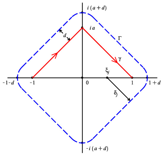
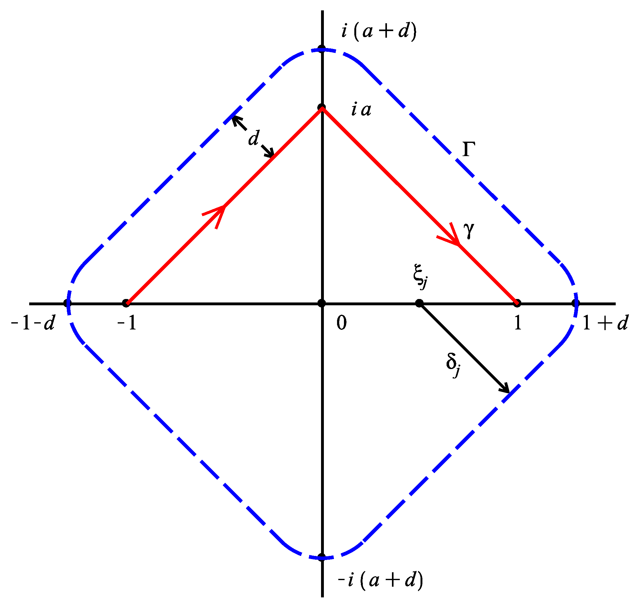
The path $\gamma$ is shown in Figure 1. By $z=t+ia\left(1-\left|t\right|\right)$,

$$\left|z-{\xi }_j\right|=\sqrt{{\left(t-{\xi }_j\right)}^2+a^2{\left(1-\left|t\right|\right)}^2}.$$

Moreover, $|e^{i\omega z}|=e^{-\omega a\left(1-\left|t\right|\right)}$, and $\left|dz\right|=\sqrt{1+a^2}dt=cdt$ on the path $\gamma$; it is true that

$$\begin{array}{c}\hfill {\int }_{\gamma }\left|\prod _{j=-n,j\ne 0}^n\left(z-{\xi }_j\right)e^{i\omega z}\right|\left|dz\right|=c{\int }_{-1}^1\prod _{j=-n,j\ne 0}^n\sqrt{{\left(t-{\xi }_j\right)}^2+a^2{\left(1-\left|t\right|\right)}^2}{e}^{-\omega a\left(1-\left|t\right|\right)}dt.\end{array}$$

Noting that ${\xi }_{-j}=-{\xi }_j\in [-1,1]$ with $j=1,2,\cdots ,n$, then ${\prod }_{j=-n,j\ne 0}^n\sqrt{{\left(t-{\xi }_j\right)}^2+a^2{\left(1-\left|t\right|\right)}^2}$ is an even function, so the above formula can be written as

$$\begin{array}{ccc}\hfill {\int }_{\gamma }\left|\prod _{j=-n,j\ne 0}^n\left(z-{\xi }_j\right)e^{i\omega z}\right|\left|dz\right|& =& 2c{\int }_0^1\prod _{j=-n,j\ne 0}^n\sqrt{{\left(t-{\xi }_j\right)}^2+a^2{\left(1-\left|t\right|\right)}^2}{e}^{-\omega a\left(1-\left|t\right|\right)}dt\hfill \\ & =& 2c{\int }_0^1\prod _{j=-n,j\ne 0}^n\sqrt{{\left(1-t-{\xi }_j\right)}^2+a^2{t}^2}{e}^{-\omega at}dt.\hfill \end{array}$$

According to the Schwartz inequality,

$${\int }_0^1\prod _{j=-n,j\ne 0}^n\sqrt{{\left(1-t-{\xi }_j\right)}^2+a^2{t}^2}{e}^{-\omega at}dt\le {\left\{{\int }_0^1\prod _{j=-n,j\ne 0}^n\left[{\left(1-t-{\xi }_j\right)}^2+a^2{t}^2\right]e^{-2\omega at}dt\right\}}^{1/2},$$

so (9) holds. Similarly, (10) holds. □

In the following two theorems, the contour $\mathsf{\Gamma }$, as shown in Figure 1, can be expressed as $\mathsf{\Gamma }={\bigcup }_{k=1}^8{\mathsf{\Gamma }}_k$, where

$${\mathsf{\Gamma }}_{1,2}=\left\{z\left|z=t-ad/c\pm id/c\pm ia(1+t),t\in [-1,0]\right.\right\},$$

$${\mathsf{\Gamma }}_{3,4}=\left\{z\left|z=t+ad/c\pm id/c\pm ia(1-t),t\in [0,1]\right.\right\},$$

$${\mathsf{\Gamma }}_{5,6}=\left\{z\left|z=\pm 1+d{e}^{i\theta },\theta \in [\mp \pi /2+arctana,\pi \mp \pi /2-arctana]\right.\right\},$$

$${\mathsf{\Gamma }}_{7,8}=\left\{z\left|z=\pm ia+d{e}^{i\theta },\theta \in [\pm \pi /2-arctana,\pm \pi /2+arctana]\right.\right\}.$$

Obviously, the length L of $\mathsf{\Gamma }$ satisfies $L=4c+2\pi d$, in which $c=\sqrt{1+a^2}$.

Theorem 5.

Suppose Γ as it is shown in Figure 1 and that U is a region enclosed by Γ. If $f\in \mathcal{O}\left(U\right)\bigcap C\left(\overline{U}\right)$ and the different even nodes satisfy ${\xi }_j=-{\xi }_{-j}\in (0,1]$ with $j=1,2,\cdots ,n$, then for all $\omega ,a\ge 0$, it is true that

$$\begin{array}{ccc}\hfill & & \left|\langle f,e^{i\omega x}\rangle -\sum _{j=-n,j\ne 0}^{n}f\left({\xi }_j\right)〈e^{i\omega x},l_j〉\right|\hfill \\ & \le & \frac{2c\left(1+\frac{2c}{\pi d}\right)M}{{\prod }_{j=1}^n{\left(\frac{a}{c}-\frac{a}{c}{\xi }_j+d\right)}^2}{\left\{{\int }_0^1\prod _{j=-n,j\ne 0}^n\left[{\left(1-t-{\xi }_j\right)}^2+a^2{t}^2\right]e^{-2\omega at}dt\right\}}^{1/2},\hfill \end{array}$$

(11)

where $c=\sqrt{1+a^2}$, $M={max}_{\zeta \in \mathsf{\Gamma }}\left|f\left(\zeta \right)\right|$, $l_j\left(x\right)={\prod }_{m=-n,m\ne j,0}^n\frac{x^2-{\xi }_m^2}{{\xi }_j^2-{\xi }_m^2}$.

Proof. 

According to Lemma 1,

$$\left|\langle f,e^{i\omega x}\rangle -\sum _{j=-n,j\ne 0}^{n}f\left({\xi }_j\right)〈e^{i\omega x},l_j〉\right|\le \frac{ML}{2\pi d{\prod }_{j=-n,j\ne 0}^n{\delta }_j}{\int }_{\gamma }\left|\prod _{j=-n,j\ne 0}^n\left(z-{\xi }_j\right)e^{i\omega z}\right|\left|dz\right|,$$

where the length $L=4c+2\pi d$. Noting the distance ${\delta }_j=inf\left\{\left|{\xi }_j-\zeta \right||{\xi }_j\in [-1,1],\zeta \in \mathsf{\Gamma }\right\}$, it is obvious that ${\delta }_j=\left(\left|a\right|-\left|a{\xi }_j\right|\right)/c+d$ with $j=\pm 1,\pm 2,\cdots ,\pm n$. Moreover, according to the inequality, (9) and (11) hold. □

Theorem 6.

Suppose Γ as it is shown in Figure 1 and that U is a region enclosed by Γ. If $f\in \mathcal{O}\left(U\right)\bigcap C\left(\overline{U}\right)$, the different odd nodes satisfy ${\xi }_j=-{\xi }_{-j}\in (0,1]$ with $j=1,2,\cdots ,n$, and ${\xi }_0=0$, then for all $\omega ,a\ge 0$, it is true that

$$\begin{array}{ccc}\hfill & & \left|\langle f,e^{i\omega x}\rangle -\sum _{j=-n}^{n}f\left({\xi }_j\right)〈e^{i\omega x},l_j〉\right|\hfill \\ & \le & \frac{2c\left(1+\frac{2c}{\pi d}\right)M}{\left(\frac{a}{c}+d\right){\prod }_{j=1}^n{\left(\frac{a}{c}-\frac{a}{c}{\xi }_j+d\right)}^2}{\left\{{\int }_0^1\prod _{j=-n}^n\left[{\left(1-t-{\xi }_j\right)}^2+a^2{t}^2\right]e^{-2\omega at}dt\right\}}^{1/2},\hfill \end{array}$$

(12)

where $c=\sqrt{1+a^2}$, $M={max}_{\zeta \in \mathsf{\Gamma }}\left|f\left(\zeta \right)\right|$, $l_j\left(x\right)={\prod }_{m=-n,m\ne j}^n\frac{x^2-{\xi }_m^2}{{\xi }_j^2-{\xi }_m^2}$.

Proof. 

According to Lemma 1,

$$\left|\langle f,e^{i\omega x}\rangle -\sum _{j=-n}^{n}f\left({\xi }_j\right)〈e^{i\omega x},l_j〉\right|\le \frac{ML}{2\pi d{\prod }_{j=-n}^n{\delta }_j}{\int }_{\gamma }\left|\prod _{j=-n}^n\left(z-{\xi }_j\right)e^{i\omega z}\right|\left|dz\right|,$$

where $L=4c+2\pi d$, and ${\delta }_j=\left(\left|a\right|-\left|a{\xi }_j\right|\right)/c+d$ with $j=-n,-n+1,\cdots ,n$. Moreover, according to the inequality (10), (12) holds. □

4. The Nodes Related to Frequency

4.1. The Nodes of ${\int }_{-1}^{1}f\left(x\right)e^{i\omega x}dx$

If the right sides of the inequalities (11) and (12) are minimized, then a is a function about $\omega$ and n. According to the theoretical analyses and numerical experiments, there are three conclusions. First, if $\omega =0$, then $a=0$, and the even nodes ${\xi }_{\mp 1},{\xi }_{\mp 2},\cdots ,{\xi }_{\mp n}$ are the roots of the $2n$-th Legendre orthogonal polynomial, or the odd nodes $0,{\xi }_{\mp 1},{\xi }_{\mp 2},\cdots ,{\xi }_{\mp n}$ are the roots of the $2n+1$-th Legendre orthogonal polynomial [7,13]. Second, a increases slowly as $\left|\omega \right|$ increases. Third, a decreases as n increases.

Therefore, for simplicity, we suggest that

$$a=\frac{\omega }{\omega +1}\frac{1}{\mathrm{Nodes}\mathrm{number}},$$

(13)

and for the even nodes,

$${\xi }_j=-{\xi }_{-j}=\frac{\omega +2n{\eta }_j}{\omega +2n},j=1,2,\cdots ,n,$$

(14)

where $\mp {\eta }_1,\mp {\eta }_2,\cdots ,\mp {\eta }_n$ are the roots of the $2n$-th Legendre orthogonal polynomial, and for the odd nodes,

$$\begin{array}{ccc}\hfill & & {\xi }_0=0,\hfill \\ & & {\xi }_j=-{\xi }_{-j}=\frac{\omega +(2n+1){\eta }_j}{\omega +2n+1},j=1,2,\cdots ,n,\hfill \end{array}$$

(15)

where $0,\mp {\eta }_1,\mp {\eta }_2,\cdots ,\mp {\eta }_n$ are the roots of the $2n+1$-th Legendre orthogonal polynomial.

4.2. The Nodes of ${\int }_{-1}^1{(1-x^2)}^{\alpha }f\left(x\right)e^{i\omega x}dx$

Similarly to Section 4.1, we suggest that a is defined as (13). If $\omega =0$, then $a=0$, and the even nodes ${\xi }_{\mp 1},{\xi }_{\mp 2},\cdots ,{\xi }_{\mp n}$ are the roots of the $2n$-th Jacobi orthogonal polynomial, or the odd nodes $0,{\xi }_{\mp 1},{\xi }_{\mp 2},\cdots ,{\xi }_{\mp n}$ are the roots of the $2n+1$-th Jacobi orthogonal polynomial with the weight ${\left(1-x^2\right)}^{\alpha }$ [7,13].

Therefore, for simplicity, we suggest that the even nodes are given as (14), where $\mp {\eta }_1,\mp {\eta }_2,\cdots ,\mp {\eta }_n$ are the roots of the $2n$-th Jacobi orthogonal polynomial with the weight ${\left(1-x^2\right)}^{\alpha }$, and the odd nodes are given as (15), where $0,\mp {\eta }_1,\mp {\eta }_2,\cdots ,\mp {\eta }_n$ are the roots of the Jacobi orthogonal polynomial with the weight ${\left(1-x^2\right)}^{\alpha }$.

5. The Expression of Coefficients with the Bessel Function

5.1. The Coefficients $〈e^{i\omega x},l_j\left(x\right)〉$

In this subsection, the coefficients $〈e^{i\omega x},l_j\left(x\right)〉$ in (2) will be expressed as follows.

• If the even nodes satisfy ${\xi }_{-j}=-{\xi }_j$ with $j=1,2,\cdots ,n$, then

$$l_j\left(x\right)=\prod _{m=-n,m\ne 0,j}^n\frac{x-{\xi }_m}{{\xi }_j-{\xi }_m}$$

can be expressed as

$$l_j\left(x\right)=\frac{1}{2}\left(\frac{x}{{\xi }_j}+1\right)\prod _{m=1,m\ne j}^n\frac{x^2-{\xi }_m^2}{{\xi }_j^2-{\xi }_m^2}$$

with $j=\mp 1,\mp 2,\cdots ,\mp n$. In addition,

$$\prod _{m=1,m\ne j}^n\left(x^2-{\xi }_m^2\right)=\sum _{m=0}^{n-1}{\beta }_{jm}{\left(x^2-1\right)}^m,$$

where ${\beta }_{jm}$ is the sum of products of all $n-m-1$ elements chosen from the set

$$\left\{1-{\xi }_1^2,\cdots ,1-{\xi }_{j-1}^2,1-{\xi }_{j+1}^2,\cdots ,1-{\xi }_n^2\right\},$$

denoted as

$${\beta }_{-j,m}={\beta }_{jm}=\sum _{\begin{array}{c}S\subseteq \{1,\cdots ,j-1,j+1,\cdots ,n\}\\ \left|S\right|=n-m-1\end{array}}\prod _{k\in S}\left(1-{\xi }_k^2\right).$$

(16)

Moreover, the following moments of Fourier integrals can be expressed by the Bessel function of the first kind [20]; if $\omega \ne 0,\alpha >-1$, then

$$\begin{array}{c}\hfill {\int }_{-1}^1{(1-x^2)}^{\alpha }{e}^{i\omega x}dx=\left\{\begin{array}{cc}\sqrt{\pi }\mathsf{\Gamma }(\alpha +1){\left(-2/\omega \right)}^{\alpha +1/2}{J}_{\alpha +1/2}(-\omega ),\hfill & arg\omega =\pi ,\hfill \\ \sqrt{\pi }\mathsf{\Gamma }(\alpha +1){\left(2/\omega \right)}^{\alpha +1/2}{J}_{\alpha +1/2}\left(\omega \right),\hfill & arg\omega \ne \pi ,\hfill \end{array}\right.\end{array}$$

and

$$\begin{array}{c}\hfill {\int }_{-1}^{1}x{(1-x^2)}^{\alpha }{e}^{i\omega x}dx=\left\{\begin{array}{cc}i\sqrt{\pi }\mathsf{\Gamma }(\alpha +1){\left(-2/\omega \right)}^{\alpha +1/2}{J}_{\alpha +3/2}(-\omega ),\hfill & arg\omega =\pi ,\hfill \\ i\sqrt{\pi }\mathsf{\Gamma }(\alpha +1){\left(2/\omega \right)}^{\alpha +1/2}{J}_{\alpha +3/2}\left(\omega \right),\hfill & arg\omega \ne \pi .\hfill \end{array}\right.\end{array}$$

If there is no segmentation, $\omega >0$ is assumed. We will not repeat this assumption below. According to the above formulas, the coefficients in (2) are

$$〈e^{i\omega x},l_j\left(x\right)〉=\frac{\sqrt{\pi }{\sum }_{m=0}^{n-1}{(-1)}^{m}m!{\beta }_{jm}{\left(\frac{2}{\omega }\right)}^{m+\frac{1}{2}}\left[{\xi }_j{J}_{m+\frac{1}{2}}\left(\omega \right)+i{J}_{m+\frac{3}{2}}\left(\omega \right)\right]}{2{\xi }_j{\prod }_{m=1,m\ne j}^n({\xi }_j^2-{\xi }_m^2)}$$

(17)

with $j=\mp 1,\mp 2,\cdots ,\mp n$.

• If the odd nodes satisfy ${\xi }_{-j}=-{\xi }_j$ with $j=1,2,\cdots ,n$ and ${\xi }_0=0$, then

$$l_j\left(x\right)=\prod _{m=-n,m\ne j}^n\frac{x-{\xi }_m}{{\xi }_j-{\xi }_m}$$

can be expressed as

$$\begin{array}{c}\hfill l_j\left(x\right)=\left\{\begin{array}{cc}\frac{1}{2}\left(\frac{x^2}{{\xi }_j^2}+\frac{x}{{\xi }_j}\right)\prod _{m=1,m\ne j}^n\frac{x^2-{\xi }_m^2}{{\xi }_j^2-{\xi }_m^2},\hfill & j\ne 0,\hfill \\ \prod _{m=1}^n\frac{x^2-{\xi }_m^2}{{\xi }_m^2},\hfill & j=0.\hfill \end{array}\right.\end{array}$$

For $j\ne 0$,

$$\prod _{m=1,m\ne j}^n\left(x^2-{\xi }_m^2\right)=\sum _{m=0}^{n-1}{\beta }_{jm}{\left(x^2-1\right)}^m,$$

where ${\beta }_{-j,m}={\beta }_{jm}$ is defined as in (16). According to the Bessel expression of the moments of Fourier integrals, the coefficients in (2) can be expressed as

$$〈e^{i\omega x},l_j\left(x\right)〉=\frac{\sqrt{\pi }{\sum }_{m=0}^{n-1}{(-1)}^{m}m!{\beta }_{jm}{\left(\frac{2}{\omega }\right)}^{m+\frac{1}{2}}\left[J_{m+\frac{1}{2}}\left(\omega \right)-\frac{2m+2}{\omega }{J}_{m+\frac{3}{2}}\left(\omega \right)+i{\xi }_j{J}_{m+\frac{3}{2}}\left(\omega \right)\right]}{2{\xi }_j^2{\prod }_{m=1,m\ne j}^n({\xi }_j^2-{\xi }_m^2)}$$

(18)

with $j=\mp 1,\mp 2,\cdots ,\mp n$. Meanwhile, for $j=0$,

$$\prod _{m=1}^n\left(x^2-{\xi }_m^2\right)=\sum _{m=0}^n{\beta }_{0,m}{\left(x^2-1\right)}^m,$$

where ${\beta }_{0,m}$ is the sum of the products of all $n-m$ elements chosen from the set $\left\{1-{\xi }_1^2,1-{\xi }_2^2,\cdots ,1-{\xi }_n^2\right\}$, denoted as

$${\beta }_{0,m}=\sum _{\begin{array}{c}S\subseteq \{1,2,\cdots ,n\}\\ \left|S\right|=n-m\end{array}}\prod _{k\in S}\left(1-{\xi }_k^2\right).$$

(19)

Therefore, the coefficients in (2) are

$$〈e^{i\omega x},l_0\left(x\right)〉=\frac{\sqrt{\pi }{\sum }_{m=0}^n{(-1)}^{m}m!{\beta }_{0,m}{\left(\frac{2}{\omega }\right)}^{m+\frac{1}{2}}{J}_{m+\frac{1}{2}}\left(\omega \right)}{{\prod }_{m=1}^n{\xi }_m^2}.$$

(20)

5.2. The Coefficients $〈{\left(1-x^2\right)}^{\alpha }{e}^{i\omega x},l_j\left(x\right)〉$

In this section, the coefficients $〈{\left(1-x^2\right)}^{\alpha }{e}^{i\omega x},l_j\left(x\right)〉$ in (3) will be expressed.

• Let the even nodes be ${\xi }_{-j}=-{\xi }_j$ with $j=1,2,\cdots ,n$. The coefficients in (3) are

$$〈e^{i\omega x},l_j\left(x\right)〉=\frac{\sqrt{\pi }{\sum }_{m=0}^{n-1}{(-1)}^m\mathsf{\Gamma }(m+\alpha +1){\beta }_{jm}{\left(\frac{2}{\omega }\right)}^{m+\alpha +\frac{1}{2}}\left[{\xi }_j{J}_{m+\alpha +\frac{1}{2}}\left(\omega \right)+i{J}_{m+\alpha +\frac{3}{2}}\left(\omega \right)\right]}{2{\xi }_j{\prod }_{m=1,m\ne j}^n({\xi }_j^2-{\xi }_m^2)}$$

(21)

with $j=\mp 1,\mp 2,\cdots ,\mp n$, where ${\beta }_{jm}$ is given as in (16).

• Let the odd nodes be ${\xi }_{-j}=-{\xi }_j$ with $j=1,2,\cdots ,n$ and ${\xi }_0=0$.

$$〈e^{i\omega x},l_j\left(x\right)〉=\frac{\sqrt{\pi }{\sum }_{m=0}^{n-1}{(-1)}^m\mathsf{\Gamma }(m+\alpha +1){\beta }_{jm}{\left(\frac{2}{\omega }\right)}^{m+\alpha +\frac{1}{2}}\left[J_{m+\alpha +\frac{1}{2}}\left(\omega \right)+\left(-2\frac{m+\alpha +1}{\omega }+i{\xi }_j\right)J_{m+\alpha +\frac{3}{2}}\left(\omega \right)\right]}{2{\xi }_j^2{\prod }_{m=1,m\ne j}^n({\xi }_j^2-{\xi }_m^2)}$$

(22)

with $j=\mp 1,\mp 2,\cdots ,\mp n$, where ${\beta }_{jm}$ is given as in (16). Meanwhile, for $j=0$, the coefficients in (2) are

$$〈e^{i\omega x},l_0〉=\frac{\sqrt{\pi }{\sum }_{m=0}^n{(-1)}^m\mathsf{\Gamma }(m+\alpha +1){\beta }_{0,m}{\left(\frac{2}{\omega }\right)}^{m+\alpha +\frac{1}{2}}{J}_{m+\alpha +\frac{1}{2}}\left(\omega \right)}{{\prod }_{m=1}^n{\xi }_m^2},$$

(23)

where ${\beta }_{0,m}$ is given as in (19).

6. The Quadrature Interpolation Formulas of ${\int }_{-\mathbf{1}}^{\mathbf{1}}\mathbf{f}\left(\mathbf{x}\right){\mathbf{e}}^{\mathbf{i}\mathbf{\omega }\mathbf{x}}\mathbf{dx}$

On one hand, by (18), the quadrature interpolation formula (2) with even nodes can be written as

$${\int }_{-1}^{1}f\left(x\right)e^{i\omega x}dx\approx \sum _{j=-n,j\ne 0}^{n}f\left({\xi }_j\right)\frac{\sqrt{\pi }{\sum }_{m=0}^{n-1}{(-1)}^{m}m!{\beta }_{jm}{\left(\frac{2}{\omega }\right)}^{m+\frac{1}{2}}\left[{\xi }_j{J}_{m+\frac{1}{2}}\left(\omega \right)+i{J}_{m+\frac{3}{2}}\left(\omega \right)\right]}{2{\xi }_j{\prod }_{m=1,m\ne j}^n({\xi }_j^2-{\xi }_m^2)},$$

(24)

where ${\beta }_{jm}$ is given as in (16).

On the other hand, by (18) and (20), the quadrature interpolation formula (2) with odd nodes can be written as

$$\begin{array}{ccc}\hfill & & {\int }_{-1}^{1}f\left(x\right)e^{i\omega x}dx\hfill \\ & \approx & f\left(0\right)\frac{\sqrt{\pi }{\sum }_{m=0}^n{(-1)}^{m}m!{\beta }_{0,m}{\left(\frac{2}{\omega }\right)}^{m+\frac{1}{2}}{J}_{m+\frac{1}{2}}\left(\omega \right)}{{\prod }_{m=1}^n{\xi }_m^2}\hfill \\ & & +\sum _{j=-n,j\ne 0}^{n}f\left({\xi }_j\right)\frac{\sqrt{\pi }{\sum }_{m=0}^{n-1}{(-1)}^{m}m!{\beta }_{jm}{\left(\frac{2}{\omega }\right)}^{m+\frac{1}{2}}\left[J_{m+\frac{1}{2}}\left(\omega \right)-\frac{2m+2}{\omega }{J}_{m+\frac{3}{2}}\left(\omega \right)+i{\xi }_j{J}_{m+\frac{3}{2}}\left(\omega \right)\right]}{2{\xi }_j^2{\prod }_{m=1,m\ne j}^n({\xi }_j^2-{\xi }_m^2)},\hfill \end{array}$$

(25)

where ${\beta }_{jm}$ is given as in (16) and ${\beta }_{0,m}$ is given as in (19).

As examples, the quadrature interpolation formulas with two, three, and four nodes are listed below.

• The quadrature formula with two nodes:

  $${\int }_{-1}^{1}f\left(x\right)e^{i\omega x}dx\approx \sum _{j=\mp 1}f\left({\xi }_j\right)\left(\frac{sin\omega }{\omega }+i\frac{sin\omega -\omega cos\omega }{{\omega }^2{\xi }_j}\right).$$

  (26)
• The quadrature formula with three nodes:

  $${\int }_{-1}^{1}f\left(x\right)e^{i\omega x}dx\approx w_{-1}f\left(-{\xi }_1\right)+w_{0}f\left(0\right)+w_{1}f\left({\xi }_1\right),$$

  (27)

  where

  $$w_0=2\frac{sin\omega }{\omega }\left(1-\frac{1}{{\xi }_1^2}\right)+4\frac{sin\omega -\omega cos\omega }{{\omega }^3}\frac{1}{{\xi }_1^2},$$

  $$w_{\mp 1}=\frac{sin\omega }{\omega }\frac{1}{{\xi }_1^2}-2\frac{sin\omega -\omega cos\omega }{{\omega }^3}\frac{1}{{\xi }_1^2}\mp i\frac{sin\omega -\omega cos\omega }{{\omega }^2}\frac{1}{{\xi }_1}.$$
• The quadrature formula with four nodes:

  $${\int }_{-1}^{1}f\left(x\right)e^{i\omega x}dx\approx \sum _{j=\mp 1,\mp 2}{w}_{j}f\left({\xi }_j\right),$$

  (28)

  where

  $$w_{\mp 1}=\frac{1}{{\xi }_1^2-{\xi }_2^2}\left((1-{\xi }_2^2){\mathsf{\Omega }}_1-{\mathsf{\Omega }}_2\mp i\frac{1-{\xi }_2^2}{{\xi }_1}{\mathsf{\Omega }}_3\pm i\frac{1}{{\xi }_1}{\mathsf{\Omega }}_4\right),$$

  $$w_{\mp 2}=\frac{1}{{\xi }_1^2-{\xi }_2^2}\left(({\xi }_1^2-1){\mathsf{\Omega }}_1+{\mathsf{\Omega }}_2\mp i\frac{{\xi }_1^2-1}{{\xi }_2}{\mathsf{\Omega }}_3\mp i\frac{1}{{\xi }_2}{\mathsf{\Omega }}_4\right),$$

  and

  $${\mathsf{\Omega }}_1=\frac{sin\omega }{\omega },{\mathsf{\Omega }}_2=2\frac{sin\omega -\omega cos\omega }{{\omega }^3},$$

  $${\mathsf{\Omega }}_3=\frac{sin\omega -\omega cos\omega }{{\omega }^2},{\mathsf{\Omega }}_4=2\frac{3sin\omega -3\omega cos\omega -{\omega }^{2}sin\omega }{{\omega }^4}.$$

7. The Quadrature Interpolation Formulas of ${\int }_{-\mathbf{1}}^{\mathbf{1}}{(\mathbf{1}-{\mathit{x}}^{\mathbf{2}})}^{\mathbf{\alpha }}\mathit{f}\left(\mathit{x}\right){\mathit{e}}^{\mathit{i}\mathit{\omega }\mathit{x}}\mathit{dx}$

On one hand, by (21), the quadrature interpolation formula (3) with even nodes can be written as

$$\begin{array}{ccc}\hfill & & {\int }_{-1}^1{(1-x^2)}^{\alpha }f\left(x\right)e^{i\omega x}dx\hfill \\ & \approx & \sum _{j=-n,j\ne 0}^{n}f\left({\xi }_j\right)\frac{\sqrt{\pi }{\sum }_{m=0}^{n-1}{(-1)}^m\mathsf{\Gamma }(m+\alpha +1){\beta }_{jm}{\left(\frac{2}{\omega }\right)}^{m+\alpha +\frac{1}{2}}\left[{\xi }_j{J}_{m+\alpha +\frac{1}{2}}\left(\omega \right)+i{J}_{m+\alpha +\frac{3}{2}}\left(\omega \right)\right]}{2{\xi }_j{\prod }_{m=1,m\ne j}^n({\xi }_j^2-{\xi }_m^2)},\hfill \end{array}$$

(29)

where ${\beta }_{jm}$ is given as in (16).

On the other hand, by (22) and (23), the quadrature interpolation formula (3) with odd nodes can be written as

$$\begin{array}{ccc}\hfill & & {\int }_{-1}^1{(1-x^2)}^{\alpha }f\left(x\right)e^{i\omega x}dx\hfill \\ & \approx & f\left(0\right)\frac{\sqrt{\pi }{\sum }_{m=0}^n{(-1)}^m\mathsf{\Gamma }(m+\alpha +1){\beta }_{0,m}{\left(\frac{2}{\omega }\right)}^{m+\alpha +\frac{1}{2}}{J}_{m+\alpha +\frac{1}{2}}\left(\omega \right)}{{\prod }_{m=1}^n{\xi }_m^2}\hfill \\ & & +\sum _{j=-n,j\ne 0}^{n}f\left({\xi }_j\right)\frac{\sqrt{\pi }{\sum }_{m=0}^{n-1}{(-1)}^m\mathsf{\Gamma }(m+\alpha +1){\beta }_{jm}{\left(\frac{2}{\omega }\right)}^{m+\alpha +\frac{1}{2}}\left[J_{m+\alpha +\frac{1}{2}}\left(\omega \right)+\left(-2\frac{m+\alpha +1}{\omega }+i{\xi }_j\right)J_{m+\alpha +\frac{3}{2}}\left(\omega \right)\right]}{2{\xi }_j^2{\prod }_{m=1,m\ne j}^n({\xi }_j^2-{\xi }_m^2)},\hfill \end{array}$$

(30)

where ${\beta }_{jm}$ is given as in (16) and ${\beta }_{0,m}$ is given as in (19).

As examples, the quadrature interpolation formulas with two, three, and four nodes are listed below.

• The quadrature formula with two nodes:

  $${\int }_{-1}^1{(1-x^2)}^{\alpha }f\left(x\right)e^{i\omega x}dx\approx \sqrt{\pi }\mathsf{\Gamma }(\alpha +1)\frac{2^{\alpha -1/2}}{{\omega }^{\alpha +1/2}}\sum _{j=\mp 1}f\left({\xi }_j\right)\left(J_{\alpha +1/2}\left(\omega \right)+i\frac{J_{\alpha +3/2}\left(\omega \right)}{{\xi }_j}\right).$$

  (31)
• The quadrature formula with three nodes:

  $${\int }_{-1}^1{(1-x^2)}^{\alpha }f\left(x\right)e^{i\omega x}dx\approx \sqrt{\pi }\mathsf{\Gamma }(\alpha +1){\left(\frac{2}{\omega }\right)}^{\alpha +1/2}\left[w_{-1}f\left(-{\xi }_1\right)+w_{0}f\left(0\right)+w_{1}f\left({\xi }_1\right)\right],$$

  (32)

  where

  $$w_0=J_{\alpha +1/2}\left(\omega \right)\left(1-\frac{1}{{\xi }_1^2}\right)+2\frac{(\alpha +1)J_{\alpha +3/2}\left(\omega \right)}{\omega {\xi }_1^2},$$

  $$w_{\mp 1}=\frac{J_{\alpha +1/2}\left(\omega \right)}{2{\xi }_1^2}-\frac{(\alpha +1)J_{\alpha +3/2}\left(\omega \right)}{\omega {\xi }_1^2}\mp i\frac{J_{\alpha +3/2}\left(\omega \right)}{2{\xi }_1}.$$
• The quadrature formula with four nodes:

$${\int }_{-1}^1{(1-x^2)}^{\alpha }f\left(x\right)e^{i\omega x}dx\approx \sqrt{\pi }\mathsf{\Gamma }(\alpha +1){\left(\frac{2}{\omega }\right)}^{\alpha +1/2}\sum _{j=\mp 1,\mp 2}{w}_{j}f\left({\xi }_j\right),$$

(33)

where

$$w_{\mp 1}=\frac{1}{{\xi }_1^2-{\xi }_2^2}\left(\frac{1-{\xi }_2^2}{2}{J}_{\alpha +\frac{1}{2}}\left(\omega \right)-\frac{\alpha +1}{\omega }{J}_{\alpha +\frac{3}{2}}\left(\omega \right)\mp i\frac{1-{\xi }_2^2}{2{\xi }_1}{J}_{\alpha +\frac{3}{2}}\left(\omega \right)\pm i\frac{\alpha +1}{\omega {\xi }_1}{J}_{\alpha +\frac{5}{2}}\left(\omega \right)\right),$$

$$w_{\mp 2}=\frac{1}{{\xi }_1^2-{\xi }_2^2}\left(\frac{{\xi }_1^2-1}{2}{J}_{\alpha +\frac{1}{2}}\left(\omega \right)+\frac{\alpha +1}{\omega }{J}_{\alpha +\frac{3}{2}}\left(\omega \right)\mp i\frac{{\xi }_1^2-1}{2{\xi }_2}{J}_{\alpha +\frac{3}{2}}\left(\omega \right)\mp i\frac{\alpha +1}{\omega {\xi }_2}{J}_{\alpha +\frac{5}{2}}\left(\omega \right)\right).$$

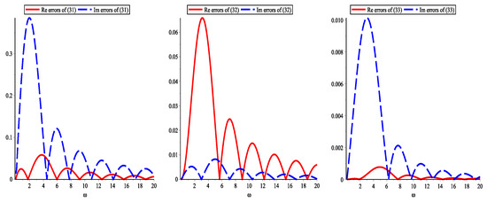
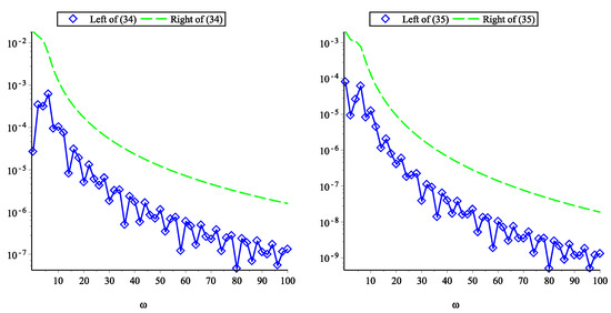
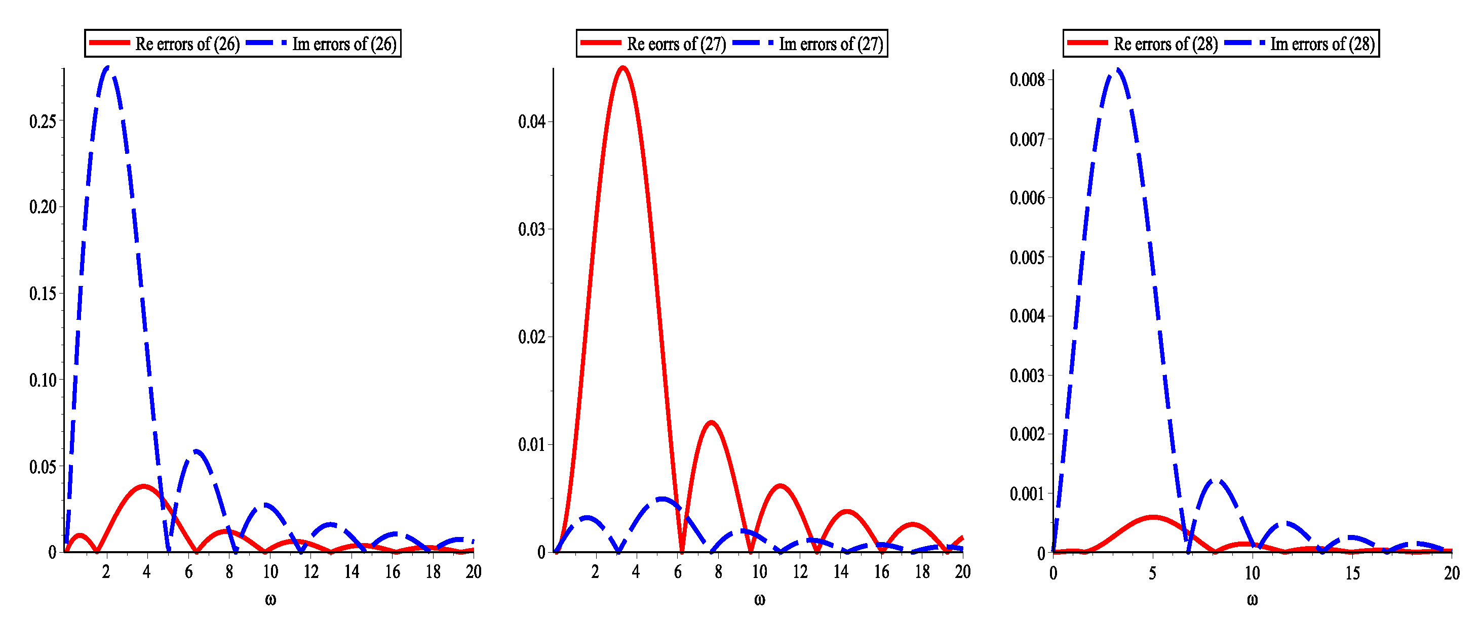
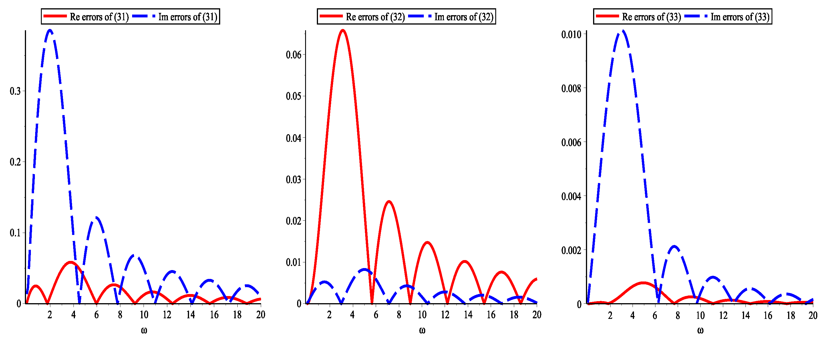
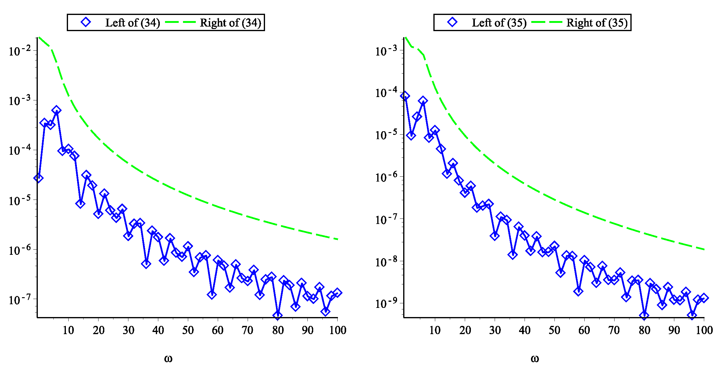
8. The Numerical Experiments

In this section, firstly, for Examples 1 and 2, we will show the real and imaginary absolute errors of ${\int }_{-1}^1{e}^{-x}{e}^{i\omega x}dx$ and ${\int }_{-1}^1{(1-x^2)}^{-1/2}{e}^{-x}{e}^{i\omega x}dx$ by using the quadrature interpolation formulas with two, three, and four nodes. Secondly, for Example 3, according to Theorems 5 and 6, we will give the absolute errors of ${\int }_{-1}^1{e}^{-x}{e}^{i\omega x}dx$ and their error bounds by using the quadrature interpolation formulas with five and six nodes. Finally, for Example 4, we will compare the errors of the six-node quadrature interpolation with those of the six-order Filon-type method.

These numerical experiments will be performed in Maple 16.

Example 1.

We consider ${\int }_{-1}^{1}f\left(x\right)e^{i\omega x}dx$. Let $f\left(x\right)=e^{-x}$. The real absolute errors of Formulas (26)–(28) are represented by real lines, and the imaginary absolute errors are represented by dashed lines in Figure 2 for $\omega \in (0,20]$, where the nodes are given as in (14) or (15).

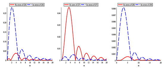
Example 2.

We consider ${\int }_{-1}^1{(1-x^2)}^{\alpha }f\left(x\right)e^{i\omega x}dx$. Let $\alpha =-1/2,f\left(x\right)=e^{-x}$. The real absolute errors of the Formulas (31)–(33) are represented by real lines, and the imaginary absolute errors are represented by dashed lines in Figure 3 for $\omega \in (0,20]$, where the nodes are given as in (14) or (15).

Example 3.

Let $f\left(x\right)=e^{-x}$. For simplicity, $\omega >0$ and $a\ge 0$ are assumed. Firstly, according to Theorem 6 and (12), $M=e^{d+1}$, and

$$\begin{array}{ccc}\hfill & & \left|{\int }_{-1}^1{e}^{-x}{e}^{i\omega x}dx-\frac{\sqrt{\pi }{\sum }_{m=0}^2{(-1)}^{m}m!{\beta }_{0,m}{\left(\frac{2}{\omega }\right)}^{m+\frac{1}{2}}{J}_{m+\frac{1}{2}}\left(\omega \right)}{{\prod }_{m=1}^2{\xi }_m^2}\right.\hfill \\ & & \left.-\sum _{j=-2,j\ne 0}^2{e}^{-{\xi }_j}\frac{\sqrt{\pi }{\sum }_{m=0}^1{(-1)}^{m}m!{\beta }_{jm}{\left(\frac{2}{\omega }\right)}^{m+\frac{1}{2}}\left[J_{m+\frac{1}{2}}\left(\omega \right)-\frac{2m+2}{\omega }{J}_{m+\frac{3}{2}}\left(\omega \right)+i{\xi }_j{J}_{m+\frac{3}{2}}\left(\omega \right)\right]}{2{\xi }_j^2{\prod }_{m=1,m\ne j}^2({\xi }_j^2-{\xi }_m^2)}\right|\hfill \\ & \le & \frac{2c^6(\pi d+2c)e^{d+1}}{\pi d{\prod }_{j=-2}^2\left(a-a{\xi }_j+cd\right)}{\left\{{\int }_0^1\prod _{j=-2}^2\left[{\left(1-t-{\xi }_j\right)}^2+a^2{t}^2\right]e^{-2\omega at}dt\right\}}^{1/2},\hfill \end{array}$$

(34)

where $c=\sqrt{1+a^2}$; the nodes are given as in (15), ${\beta }_{jm}$ is given as in (16) with $j=1,2$, and ${\beta }_{0,m}$ is given as in (19).

Secondly, according to Theorem 5 and (11), $M=e^{d+1}$, and

$$\begin{array}{ccc}\hfill & & \left|{\int }_{-1}^1{e}^{-x}{e}^{i\omega x}dx-\sum _{j=-3,j\ne 0}^3{e}^{-{\xi }_j}\frac{\sqrt{\pi }{\sum }_{m=0}^1{(-1)}^{m}m!{\beta }_{jm}{\left(\frac{2}{\omega }\right)}^{m+\frac{1}{2}}\left[{\xi }_j{J}_{m+\frac{1}{2}}\left(\omega \right)+i{J}_{m+\frac{3}{2}}\left(\omega \right)\right]}{2{\xi }_j{\prod }_{m=1,m\ne j}^2({\xi }_j^2-{\xi }_m^2)}\right|\hfill \\ & \le & \frac{2c^7(\pi d+2c)e^{d+1}}{\pi d{\prod }_{j=-3,j\ne 0}^3\left(a-a{\xi }_j+cd\right)}{\left\{{\int }_0^1\prod _{j=-3,j\ne 0}^3\left[{\left(1-t-{\xi }_j\right)}^2+a^2{t}^2\right]e^{-2\omega at}dt\right\}}^{1/2},\hfill \end{array}$$

(35)

where $c=\sqrt{1+a^2}$ the nodes are given as in (14), and ${\beta }_{jm}$ is given as in (16) with $j=1,2,3$.

As shown in Figure 4, the absolute errors of the quadrature interpolation formulas on the left side of the inequalities (34) and (35) are represented by diamond points for $\omega =0.1+2k$ with $k=0,1,\cdots ,50$. In addition, when $d=4.5$ or $d=6$, the right sides of (34) and (35) are taken as the error bounds, as shown by the dashed lines for $\omega =0.1+2k$ with $k=0,1,\cdots ,50$.

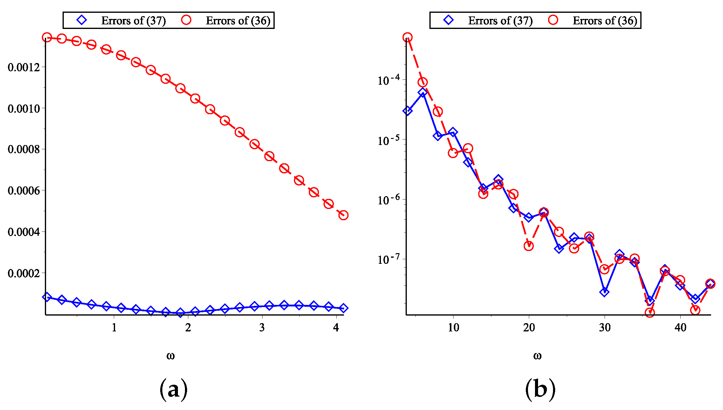
Example 4.

In recent years, Fourier integrals have usually been approximated with Filon-type methods [10,16]. A Filon-type method of the $2n+2$ order can be defined as

$${\int }_{-1}^{1}f\left(x\right)e^{i\omega x}dx\approx {\int }_{-1}^1{p}_{2n+1}\left(x\right)e^{i\omega x}dx,f\in C^{\infty }[-1,1],$$

where $p_{2n+1}\left(x\right)$ is the $2n+1$-th Hermite interpolation polynomial of $f\left(x\right)$ satisfying

$$p_{2n+1}^{\left(k\right)}(-1)=f^{\left(k\right)}(-1),p_{2n+1}^{\left(k\right)}\left(1\right)=f^{\left(k\right)}\left(1\right),k=0,1,\dots ,n.$$

These can be expressed as Bessel expansions [20]. For $f\left(x\right)=e^{-x}$, the six-order Filon-type formula is

$${\int }_{-1}^1{e}^{-x}{e}^{i\omega x}dx\approx \sqrt{\pi }\sum _{k=0}^{2}k!{\left(\frac{2}{\omega }\right)}^{k+1/2}\left[a_k{J}_{k+\frac{1}{2}}\left(\omega \right)+i{b}_k{J}_{k+\frac{3}{2}}\left(\omega \right)\right],$$

(36)

where $a_0=\frac{e+e^{-1}}{2},a_1=\frac{e^{-1}-e}{4},a_2=\frac{e^{-1}}{8}$ and $b_0=\frac{-e+e^{-1}}{2},b_1=\frac{e^{-1}}{2},b_2=\frac{7e^{-1}-e}{16}$.

On the other hand, according to (24), the quadrature interpolation formula with six nodes is

$${\int }_{-1}^1{e}^{-x}{e}^{i\omega x}dx\approx \sum _{j=-3,j\ne 0}^3{e}^{-{\xi }_j}\frac{\sqrt{\pi }{\sum }_{m=0}^2{(-1)}^{m}m!{\beta }_{jm}{\left(\frac{2}{\omega }\right)}^{m+\frac{1}{2}}\left[{\xi }_j{J}_{m+\frac{1}{2}}\left(\omega \right)+i{J}_{m+\frac{3}{2}}\left(\omega \right)\right]}{2{\xi }_j{\prod }_{m=1,m\ne j}^3({\xi }_j^2-{\xi }_m^2)},$$

(37)

where the nodes are given as in (14) with $j=1,2,3$.

Error comparisons between Filon-type formula (36) and the quadrature interpolation formula (37) are shown in Figure 5, where the absolute errors of (36) are represented by circular points and the those of (37) are represented by diamond points for $\omega =0.1+0.2k$ or $\omega =4+2k$ with $k=0,1,\cdots ,20$. These numerical experiments show that the quadrature interpolation formula in (37) is better than the Filon-type formula (36) from a low frequency to a medium frequency, and (37) is as good as (36) from a medium frequency to a high frequency. More importantly, there are no derivatives in the quadrature interpolation formula.

9. Conclusions

In this paper, according to the error bounds established by complex analysis, we studied the quadrature interpolation formula of a Fourier integral with Jacobi symmetrical weight, where the nodes and coefficients depend on frequency. For a fixed number of nodes, the formula for changing quadrature nodes is efficient regardless of whether the frequency is low or high. It is expected that the changing quadrature nodes can be generated in other ways. We will study these in the future.

References

- Filon, L.N.G. On a quadrature formula for trigonometric integrals. Proc. R. Soc. Edinb. 1928, 49, 38–47. [Google Scholar] [CrossRef]
- Chawla, M.M.; Jain, M.K. Asymptotic error estimates for the Gauss quadrature formula. Math. Comp. 1968, 22, 91–97. [Google Scholar] [CrossRef]
- Rabinowitz, P. Gaussian integration of functions with branch points singularities. Int. J. Comput. Math. 1968, 2, 625–638. [Google Scholar] [CrossRef]
- Piessens, R. Gaussian Quadrature Formulas for the Integration of Oscillating Functions. ZAMM 1970, 50, 698–700. [Google Scholar] [CrossRef]
- Piessens, R.; Branders, M. The evaluation and application of some modified moments. BIT Numer. Math. 1973, 13, 443–450. [Google Scholar] [CrossRef]
- Kzaz, M. Convergence acceleration of some Gaussian quadrature formula for analytic functions. Appl. Numer. Math. 1992, 10, 481–496. [Google Scholar] [CrossRef]
- Sobolev, S.L.; Vaskevich, V. The Theory of Cubature Formulas; Springer Science & Business Media: Berlin/Heidelberg, Germany, 1997; Volume 415. [Google Scholar]
- Bolinder, E.F. The Fourier integral and its applications. Proc. IEEE 2005, 51, 267. [Google Scholar] [CrossRef]
- Gradshteyn, I.S.; Ryzhik, I.M. Table of Integrals, Series, and Products, 7th ed.; Elsevier/Academic Press: Amsterdam, The Netherlands, 2007. [Google Scholar]
- Xiang, S.H. Efficient Filon-type methods for . BIT Numer. Math. 2007, 105, 633–658. [Google Scholar] [CrossRef]
- Trefethen, L.N. Is Gauss quadrature better than Clenshaw-Curtis? SIAM Rev. 2008, 50, 67–87. [Google Scholar] [CrossRef]
- Boykov, I.V.; Ventsel, E.S.; Boykova, A.I. An approximate solution of hypersingular integral equations. Appl. Numer. Math. 2010, 60, 607–628. [Google Scholar] [CrossRef]
- Brass, H.; Petras, K. Quadrature Theory: The Theory of Numerical Integration on a Compact Interval; American Mathematical Society: Providence, RI, USA, 2011. [Google Scholar]
- Xiang, S.; Bornemann, F. On the convergence rates of Gauss and Clenshaw-Curtis quadrature for functions of limited regularity. SIAM J. Numer. Anal. 2012, 50, 2581–2587. [Google Scholar] [CrossRef] [Green Version]
- He, G.; Zhang, C. On the numerical approximation for Fourier-type highly oscillatory integrals with Gauss-type quadrature rules. Appl. Math. Comp. 2017, 308, 96–104. [Google Scholar] [CrossRef]
- Deaño, A.; Huybrechs, D.; Iserles, A. Computing Highly Oscillatory Integrals; SIAM: Philadelphia, PA, USA, 2018. [Google Scholar]
- Wang, H. On the convergencerate of Clenshaw-Curtis quadrature for integrals with algebraic endpoint singularities. J. Comput. Appl. Math. 2018, 333, 87–98. [Google Scholar] [CrossRef]
- Kang, H. Efficient calculation and asymptotic expansions of many different oscillatory infinite integrals. Appl. Math. Comp. 2019, 346, 305–318. [Google Scholar] [CrossRef]
- Huybrechs, D.; Kuijlaars, A.; Lejon, N. A numerical method for oscillatory integrals with coalescing saddle points. SIAM J. Numer. Anal. 2019, 57, 2707–2729. [Google Scholar] [CrossRef] [Green Version]
- Zhou, Y.; Zhao, Z. The Bessel expansion of Fourier integral on finite interval. Symmetry 2019, 11, 607. [Google Scholar] [CrossRef] [Green Version]
- Liu, G.; Xiang, S. Clenshaw-Curtis-type quadrature rule for hypersingular integrals with highly oscilltory kernels. Appl. Math. Comput. 2019, 340, 251–267. [Google Scholar]
- Arama, A.; Xiang, S.; Khan, S. On the Convergence Rate of Clenshaw-Curtis Quadrature for Jacobi Weight Applied to Functions with Algebraic Endpoint Singularities. Symmetry 2020, 12, 716. [Google Scholar] [CrossRef]
Publisher’s Note: MDPI stays neutral with regard to jurisdictional claims in published maps and institutional affiliations. |
© 2022 by the authors. Licensee MDPI, Basel, Switzerland. This article is an open access article distributed under the terms and conditions of the Creative Commons Attribution (CC BY) license (https://creativecommons.org/licenses/by/4.0/).