Evaluation of Parameter Identification of a Real Manipulator Robot

Abstract

Given the widespread use of the Kalman filter in robotics, an increasing number of researchers devote themselves to its study and application. This work underscores the importance of this filter while analyzing the modifications made to the same to improve its performance and reduce its deficiencies in some fields and presenting some of its applications in robotics. The following methods are presented in this study: least squares (LS), Hopfield Neural Networks (HNN), Extended Kalman filter (EKF), and Unscented Kalman filter (UKF). These methods are used in the parameter identification of a Selective Compliant Assembly Robot Arm (SCARA) robot with 3-Degrees of Freedom (3-DoF) and a clamp at its end. The dynamic model of this robot is obtained and employed to identify its parameters; then, the identification results are compared considering the difference between the obtained parameters and the real values of the robot parameters; in this comparison, the good results yielded by the LS and UKF method stand out. Subsequently, the obtained parameters through each method are validated by measuring different performance indexes—during trajectory tracking—such as: Residual Mean Square Error (RMSE), Integral of the Absolute Error (IAE), and the Integral of the Square Error (ISE). In this way, a comparison of the robot’s performance is possible.

1. Introduction

Since dynamic systems abound in our environment, system identification techniques have gained relevance in diverse fields of knowledge, for example, engineering, economy, and biotechnology, which require an accurate model for analysis, prediction, simulation, design, and control purposes.

Particularly for system analysis and design, current control techniques require mathematical models that are increasingly precise. In many cases, these models cannot be obtained easily based on the laws governing the dynamic behavior of each system. In these cases, the Identification of Dynamic Systems plays a decisive role. This is a tool that provides the necessary approximation methods for obtaining the sought mathematical models in a relatively easy way, as well as estimating the parameters of the system under study.

Estimating the value of the dynamic parameters of the system can be calculated through different estimators, among which are the least-squares estimation, the maximum likelihood principle, neural networks, and the Kalman filter (KF).

Specifically, the Kalman filter, since its creation in 1960, has been based on the estimation of the non-observable state variables through the observed variables, which can have measurement errors [1].

The Kalman filter performs better than other estimation algorithms as it requires a small storage capacity and has a wide range of uses. Nevertheless, in actual applications, factors such as effect on the environment, incorrect parameters, and measurement errors produce errors in the system [2]. Different variations of this filter have been developed in recent years, which attempt to address the issues presented by the algorithm as a consequence of increased equipment complexity that requires enhanced efficiency and accuracy in some processes in the manufacturing, medicine, and navigation industries.

This filter has suffered several modifications that allow it to be used in diverse engineering areas, especially in robotics. Among the most relevant modifications are the Extended Kalman filter (EKF), which can be used in non-linear systems by conducting a system linearization; the Unscented Kalman filter (UKF), which is based on the premise that it is easier to approximate a probability distribution than an arbitrary linear transformation, using the Unscented Transformation (UT) for this purpose [3]. However, some modifications based on the adaptability feature, such as the Adaptive Extended Kalman filter (AEKF) and Adaptive Unscented Kalman filter (AUKF), have also been developed to determine the statistical parameters of the dynamic system according to the behavior of the system during data processing [4]. Furthermore, filters for countering undesired responses such as inconsistency from the EKF have been created.

Localization is among the most used applications of the KF and its modifications [5,6,7]. This application is employed to correct the position of some robots [8,9,10], for trajectory tracking [11,12,13,14], and for parameter estimation [15,16,17].

Recently, the KF has been applied in sensor-less speed control, which seeks to control a synchronous reluctance motor [18]. Variations of the KF have also been employed in solving one of the main challenges presented by real-time image and video processing applications, i.e., following objects and detecting movement [19].

2. Materials and Methods

2.1. Kalman Filter for Linear Systems

As an algorithm, the KF comprises two types of equation: the first type is called main equations, which associate state variables with observable variables, while the second type, called state equations, is related to the temporary structure of state variables.

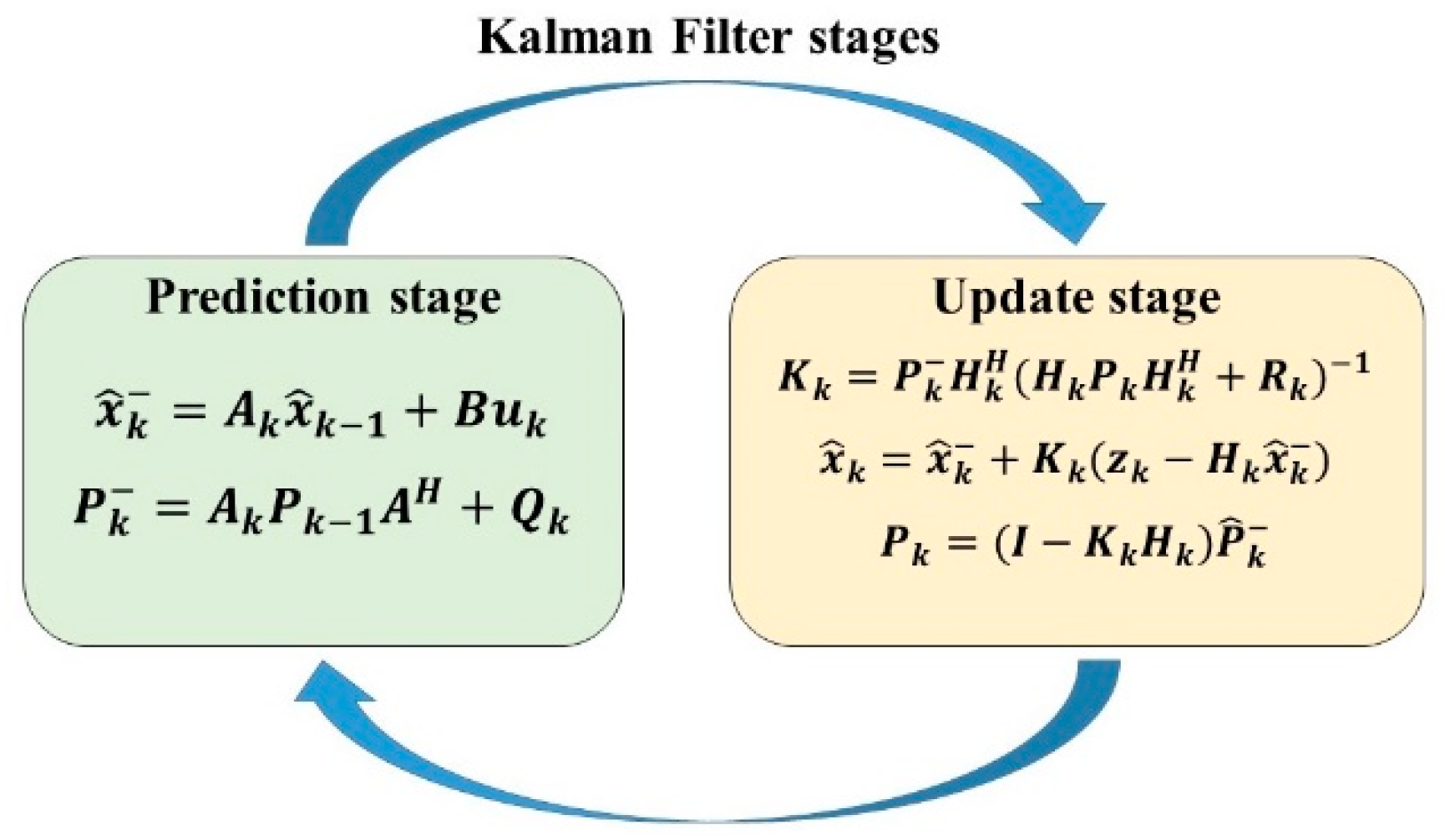
State variables are estimated by calculating time and dimension, which represent the dynamics of estate variables, but also by measuring the values of observable variables at each time instant (transversal). In conclusion, two steps explain this dynamic (see Figure 1):

• Prediction stage: state variables are estimated through their own dynamics.
• Correction stage: the first estimation is improved based on information from observable variables.

The Kalman filter is very attractive due to its recursion, i.e., its suitability for real-time use. When the new state is predicted by the algorithm at the moment t, a correction term is added, and the new state, which has been corrected, becomes an initial condition for the next stage, t + 1. In other words, in addition to the information from the state previous to estimation, available information is also used to estimate the state variables, which is denominated “signal extraction”.

The KF represents a belief or trust in the x_k state at time k that is given by the mean, ${\widehat{x}}_k^{-}$ and the $P_k^{-}$ covariance. The entry received by KF is the belief in time k − 1, represented by ${\widehat{x}}_{k-1}$ and $P_{k-1}$. The KF also needs control signals (u_k) and environment observations from the sensors (z_k) to update this belief. The output of the KF would be the belief in the time instant k, which is represented by ${\widehat{x}}_k$ and P_k.

Figure 1 shows the equations that describe the KF, which consists of two stages. In the prediction stage, the state and covariance of the error are projected in the current instant t, i.e., it is the sum to the system of instant t − 1 that was generated from the instant before the current. The second stage, or update stage, considers the observed characteristics. At this stage, based on the estimation from the prediction stage, an estimation of the characteristic location can be conducted, and thereby, a correction can be applied to the system. The new characteristics added to the map are useful for later reobservation, which can be conducted using information about the current characteristics of the system and about the association between new and old characteristics.

According to the definitions of the matrices in Figure 1:

• A_k: Matrix n × n related to the states at instant t − 1 and at instant t, without control signals.
• B_k: Matrix n × l related to control signals that are optional to the current state.
• Q_k: Matrix n × n representing process noise, or constant covariance.
• H_k: Matrix m × n that associates the current state and environment observations.
• R_k: Matrix m × m that indicates the covariance of noise in observations.
• K_k: Matrix n × m that indicates the Kalman gain, which is trust in the observed characteristics, based on the uncertainty of all characteristics together plus a data quality measurement.

The Kalman filter has been applied in a wide range of technologies. Vehicle guidance, navigation, and control are common applications of the KF, particularly in aircrafts and exploration robots. Furthermore, this filter has also expanded its use to signal processing and econometrics.

As described above, the Kalman filter is an estimation method whose parameters are corrected for each iteration based on the prediction error from the previous iteration [20]. In its original form, the KF is known to be unable to deal with state estimations correctly if employed in non-linear systems. Therefore, its extension was developed by R. Kalman, Dr. Schmidt, and the research team of the Dynamic Analysis Branch of NASA [21]. The Extended Kalman filter has an algorithm with the same recursive steps as linear Kalman filter, i.e., prediction and correction, but Taylor’s linearization is conducted during the prediction stage instead, as shown in Figure 2, where A and W are the Jacobian matrices from the partial derivatives of function f, while H and V correspond to the Jacobian matrices from the partial derivatives of function h.

2.2. Unscented Kalman Filter

The Unscented Transform is a method for calculating the statistics of a random variable that suffers a non-linear transformation [20].

If it is considered the possibility of propagating a random variable x (of L dimensions) a through a y = g(x) non-linear function, and assuming that x has a mean $\overline{x}$ and a covariance P_x, to calculate the statistics of y, a matrix X of 2L + 1 X_i sigma vectors can be formed (with its W_i corresponding weights) according to the following equations:

$$X_0=\overline{x}$$

(1)

$$X_i=\overline{x}+{\left(\sqrt{\left(L+\gamma \right)P_x}\right)}_i\hspace{1em}i=1,\dots ,L$$

(2)

$$X_i=\overline{x}-{\left(\sqrt{\left(L+\gamma \right)P_x}\right)}_i-L\hspace{1em}i=L+1,\dots ,2L$$

(3)

$$W_0^{\left(m\right)}=\frac{\gamma }{L+\gamma }$$

(4)

$$W_0^{\left(c\right)}=\frac{\gamma }{L+\gamma }+\left(1-{\alpha }^2+\beta \right)$$

(5)

$$W_i^{\left(m\right)}=W_i^{\left(c\right)}=\frac{\gamma }{2\left(L+\gamma \right)}\hspace{1em}i=1,\dots , 2L$$

(6)

where γ = α² (L + K) − L is a scaling parameter, α determines the distribution of the sigma points around the $\overline{x}$ mean—which is normally a positive value—K is a secondary scaling parameter—which should be higher or equal to 0—β is a parameter employed for obtaining previous knowledge of the x distribution—whose optimal value for Gaussian distributions is β = 2—and ${\left(\sqrt{\left(L+\gamma \right)P_x}\right)}_i$ is the i-th row of the matrix square. Sigma vectors propagate according to the following non-linear function:

$$Y_i=g\left(X_i\right)\hspace{1em}i=1,\dots ., 2L.$$

(7)

In turn, the mean and covariance of Y can be approximated using a weighed sample mean and the covariance of the posterior sigma points, according to:

$$\overline{y}={\displaystyle \sum }_{i=0}^{2L}{W}_i^{\left(m\right)}{Y}_i$$

(8)

$$P_y={\displaystyle \sum }_{i=0}^{2L}{W}_i^{\left(c\right)}\left(Y_i-\overline{y}\right){\left(Y_i-\overline{y}\right)}^T$$

(9)

It is necessary to consider that this method substantially differs from general state “sampling” methods such as the Monte-Carlo methods in terms of the particle filter, which at some point may require more sample points to propagate an accurate distribution that is likely non-Gaussian.

Each sigma point is used in the state evolution model, and, thereby, it is possible to obtain the sigma points of the predicted state based on the following equation:

$$X_k^{-}=f\left(X_{k-1},u_{k-1}\right)$$

(10)

Subsequently, the weighed measure and the covariance of the predicted sigma points are obtained according to:

$${\widehat{X}}_k^{-}={\displaystyle \sum }_{i=0}^{2L}{W}_i\left(X_{i,k}^{-}\right)$$

(11)

$$P_{x_k}^{-}={\displaystyle \sum }_{i=0}^{2L}{W}_i\left(X_{i,k}^{-}-X_k^{-}\right){\left(X_{i,k}^{-}-X_k^{-}\right)}^T$$

(12)

The predicted sigma points are used in the measurement equation for generating the predicted measurement sigma points in the following way:

$${\delta }_k^{-}=h\left(X_k^{-},u_k\right)$$

(13)

The weighted mean of the predicted measurement, the corresponding covariance matrix, and the cross-correlation matrix are calculated as follows:

• The matrix $P_{x_k{y}_k}^{-}$ represents the cross-correlation between the difference of the sigma points of the predicted state $X_{i,k}^{-}$ and corresponding predicted state ${\widehat{X}}_k$, and the difference between the sigma points of the predicted measurement ${\delta }_k^{-}$ and the corresponding predicted measurement $y_k^{-}$:

  $${\widehat{y}}_k^{-}={{\displaystyle \sum }}_{i=0}^{2L}{W}_i\left({\delta }_{i,k}^{-}\right)$$

  (14)

  $$P_{y_k}^{-}={\displaystyle \sum }_{i=0}^{2L}{W}_i\left({\delta }_k^{-}-y_k^{-}\right){\left({\delta }_k^{-}-y_k^{-}\right)}^T+R$$

  (15)

  $$P_{x_k{y}_k}^{-}={\displaystyle \sum }_{i=0}^{2L}{W}_i\left(X_{i,k}^{-}-X_k^{-}\right){\left({\delta }_k^{-}-y_k^{-}\right)}^T$$

  (16)
• Finally, the Kalman gain matrix $K_k$ is calculated to find the mean ${\widehat{X}}_k$ and the covariance matrix $P_{X_k}$ as indicated below:

  $$K_k=P_{x_k{y}_k}^{-}{\left(P_{y_k}^{-}\right)}^{-1}$$

  (17)

  $${\widehat{X}}_k=X_k^{-}+K_k\left(y_k-y_k^{-}\right)$$

  (18)

  $$P_{X_k}=P_{x_k}^{-}-K_k{P}_{y_k}^{-}{K}_k$$

  (19)

2.3. Parameters Identification and System under Study

Automation systems are present in a wide range of industrial applications, in which the inclusion of robotics is increasingly important for tasks such as manipulation and transport of elements. The growing need for manipulator robots in this industry to execute tasks with more accuracy and promptness requires the development of more exact mathematical models, which allows for a better representation of the kinematic and dynamic behavior of such robots. Therefore, the parameters employed in the dynamic model of the manipulator robot are relevant to model-based control algorithms in order to validate simulation results and to improve the accuracy of the algorithms that permit these robots to plan trajectories [22].

Parameter identification is used in the creation of mathematical models and controllers [23,24,25]. The proper selection of parameter estimation methods for robotized systems directly impacts the accuracy of these systems. Therefore, the comparison of the behavior of diverse identification methods assists in the development of more accurate and better controllers.

Through identifiability, a single parameter set is found, which is able to describe the behavior of the mathematical model [26]. This is achieved by means of data compiled from diverse experiments conducted in real systems, thanks to which it is possible to find a single solution for each unknown parameter of a mathematical model [27]. The parameter identification process of a manipulator robot starts with the gathering of input/output data from the signals that excite the robot when this executes a function or trajectory. Since, in a dynamic model, not all parameters have the same relevance, they cannot be estimated all at once. This impossibility occurs because the links of a manipulator robot contain redundant parameters that impede finding a single solution for each unknown parameter of its mathematical model. However, the non-redundant and identifiable parameters can be represented through a minimal set of dynamic parameters, whose values are useful for the development of a mathematical model. This set of parameters is denominated by base dynamic parameters or minimal dynamic parameters and is enough to describe the dynamic behavior of a mechanical system [28,29].

After parameter identification, the mathematical model needs to be validated to verify that the model properly represents the real system. The diagram in Figure 3 shows a two-stage mathematical model, in which the first stage corresponds to trajectory validation, and the second is the comparison of measured and estimated torques/forces and the calculation of the executed trajectories [22].

2.4. System under Study

The system under study corresponds to a SCARA manipulator robot with 3-DoF, which has a clamp on its end. Its first two joints are rotational, while the third one is prismatic. This robot was designed and implemented in the Laboratory of Robotics at the Electric Engineering Department of the University of Santiago of Chile for research and educational purposes (see Figure 4).

Dynamics is a branch of physics that studies the forces/torques that cause the movement of bodies. The following dynamic models are obtained from these forces/torques [31]:

• Direct Dynamic Model: Expresses the evolution of a robot’s joint coordinates over time based on the forces/torques that intervene.
• Inverse Dynamic Model: Expresses the forces/torques that intervene based on joint coordinates and their derivatives.

2.4.1. Newton–Euler Formulation

This formulation is based on the equilibrium of the forces/torques in a link, which can be represented by two equations: Newton’s motion Equation (20) and Euler’s motion Equation (21) [32].

$${\displaystyle \sum }F=m\dot{v}$$

(20)

$${\displaystyle \sum }T=I\dot{\omega }+\omega \times \left(I\omega \right)$$

(21)

where F represents the linear force, m the mass of the body, v corresponds to linear speed, I is the inertia tensor, ω is angular speed, $\dot{\omega }$ is angular acceleration, and T is the torque.

2.4.2. Lagrange–Euler Formulation

This formulation describes the behavior of a dynamic system in terms of work and energy stored in it. The closed-form equations can be systematically derived in any coordinate system [33].

The Lagrangian L is defined as:

$$L\left(q_i,{\dot{q}}_i\right)=T-U$$

(22)

From the Lagrangian, the motion equations of the dynamic system are given by:

$$\frac{d}{dt}\frac{\partial L}{\partial {\dot{q}}_i}-\frac{\partial L}{\partial q_i}=Q_i$$

(23)

where L represents the Lagrangian function, T the kinetic energy, U the potential energy, q_i the generalized coordinates, Q_i represents the generalized force applied to q_i.

Finally, the general form of the dynamic model of a manipulator robot can be expressed as:

$$\tau =M\left(q\right)\ddot{q}+C\left(q,\dot{q}\right)\dot{q}+G\left(q\right)$$

(24)

where:

• $\tau$: Generalized forces vector.
• $q$: Generalized coordinates vector.
• $M\left(q\right)$: Inertia matrix.
• $C\left(q,\dot{q}\right)$: Centrifuge and Coriolis forces vector.
• $G\left(q\right)$: Gravitational force vector.

2.4.3. Dynamic Model of the Manipulator Robot

Figure 5 shows the parameters of the system under study, based on which a dynamic model of the manipulator robot will be obtained by applying the Lagrange–Euler formulation.

where:

• m₁: First link mass.
• M₂: Second link mass.
• M₃: Third link mass.
• L₁: First link length.
• L₂: Second link length.
• L₃: Third link length.
• L_c1: Length from the first link origin to its center of mass.
• L_c2: Length from the second link origin to its center of mass.
• L_c3: Length from the third link origin to its center of mass.
• I₁: Moment of inertia of first link.
• I₂: Moment of inertia of second link.
• I₃: Moment of inertia of third link.

For the 3-DoF SCARA manipulator robot, the generalized coordinates vector is:

$$q=\left|\begin{array}{c}{\theta }_1\\ {\theta }_2\\ d_3\end{array}\right|$$

(25)

$$r_{0,c1}=\left|\begin{array}{c}{l}_{c1}\cos \left({\theta }_1\right)\\ l_{c1}\mathrm{sen}\left({\theta }_1\right)\\ l_0\end{array}\right|$$

(26)

$$r_{0,c2}=\left|\begin{array}{c}{l}_1\cos \left({\theta }_1\right)+l_{c2}\cos \left({\theta }_1+{\theta }_2\right)\\ l_1\mathrm{sen}\left({\theta }_1\right)+l_{c2}\mathrm{sen}\left({\theta }_1+{\theta }_2\right)\\ l_0\end{array}\right|$$

(27)

$$r_{0,c3}=\left|\begin{array}{c}{l}_1\cos \left({\theta }_1\right)+l_2\cos \left({\theta }_1+{\theta }_2\right)\\ l_1\mathrm{sen}\left({\theta }_1\right)+l_2\mathrm{sen}\left({\theta }_1+{\theta }_2\right)\\ l_0-d_3\end{array}\right|$$

(28)

Then, from Equations (25)–(28), the Jacobian matrixes for m₁, m₂, and m₃ are respectively calculated.

$$J_{vc1}=\left|\begin{array}{ccc}-l_{c1}\mathrm{sen}\left({\theta }_1\right)& 0& 0\\ l_{c1}\cos \left({\theta }_1\right)& 0& 0\\ 0& 0& 0\end{array}\right|$$

(29)

$$J_{vc2}=\left|\begin{array}{ccc}-l_1\mathrm{sen}\left({\theta }_1\right)-l_{c2}\mathrm{sen}\left({\theta }_1+{\theta }_2\right)& -l_{c2}\mathrm{sen}\left({\theta }_1+{\theta }_2\right)& 0\\ l_1\cos \left({\theta }_1\right)+l_{c2}\cos \left({\theta }_1+{\theta }_2\right)& -l_{c2}\cos \left({\theta }_1+{\theta }_2\right)& 0\\ 0& 0& 0\end{array}\right|$$

(30)

$$J_{vc3}=\left|\begin{array}{ccc}-l_1\mathrm{sen}\left({\theta }_1\right)-l_2\mathrm{sen}\left({\theta }_1+{\theta }_2\right)& -l_{c2}\mathrm{sen}\left({\theta }_1+{\theta }_2\right)& 0\\ l_1\cos \left({\theta }_1\right)+l_2\cos \left({\theta }_1+{\theta }_2\right)& -l_{c2}\cos \left({\theta }_1+{\theta }_2\right)& 0\\ 0& 0& -1\end{array}\right|$$

(31)

From these Jacobian matrixes, the kinetic and potential energy of the robot can be obtained, using the following equations:

$$T=\frac{1}{2}m{v}^T+\frac{1}{2}{\omega }^{T}I\omega$$

(32)

$$U=mg\stackrel{\rightharpoonup }{r}$$

(33)

Therefore, employing Equation (22), the corresponding Lagrangian for this robot will be given by the following equation:

$$L=T_1+T_2+T_3-U_1-U_2-U_3$$

(34)

Now, substituting the corresponding values in Equation (34), it is obtained:

$$\begin{array}{cc}L=& \frac{1}{2}[m_1{l}_{c1}^2+m_2\left(l_1^2+l_{c2}^2+2l_1{l}_{c2}cos{\theta }_2\right)\hfill \\ & +m_3\left(l_1^2+l_2^2+2l_1{l}_{2}cos{\theta }_2\right)+I_1+I_2\hfill \\ & +I_3]{\dot{\theta }}_1^2\hfill \\ & +[m_2{l}_{c2 }\left(l_{c2}+l_{1}cos{\theta }_2\right)+m_3\left(l_1{l}_{2}cos{\theta }_2+l_2^2\right)\hfill \\ & +I_2+I_3]{\dot{\theta }}_1{\dot{\theta }}_2+\frac{1}{2}\left[m_2{l}_{c2}^2+m_3{l}_2^2+I_3\right]{\dot{\theta }}_2^2\hfill \\ & +\frac{1}{2}{m}_3{\dot{d}}_3^2-g\left[\left(m_1+m_2\right)l_0+m_3(l_0-d_3)\right]\hfill \end{array}$$

(35)

When calculating total and partial derivatives, specified in Equation (23), the following equations describing the dynamics of the manipulator robot are obtained:

$${\tau }_1=M_{11}{\ddot{\theta }}_1+M_{12}{\ddot{\theta }}_2-2h{\dot{\theta }}_1{\dot{\theta }}_2-h{\dot{\theta }}_2{}^2$$

(36)

$${\tau }_2=M_{11}{\ddot{\theta }}_1+M_{22}{\ddot{\theta }}_2+h{\dot{\theta }}_1{}^2$$

(37)

$$F_3=M_{33}{\ddot{d}}_3+G$$

(38)

where:

$$M_{11}=m_1{l}_{c1}^2+m_2\left(l_1^2+l_{c2}^2+2l_1{l}_{c2}\cos ({\theta }_2)\right)+m_3\left(l_1^2+l_2^2+2l_1{l}_2\cos {\theta }_2\right)+I_1+I_2+I_3$$

(39)

$$M_{12}=m_2{l}_{c2}\left(l_{c2}+l_1\cos \left({\theta }_2\right)\right)+m_3\left(l_1{l}_2\cos \left({\theta }_2\right)+l_2{}^2\right)+I_2+I_3$$

(40)

$$h=\left(m_2{l}_1{l}_{c2}+m_3{l}_1{l}_2\right)\sin ({\theta }_2)$$

(41)

$$M_{22}=m_2{l}_{c2}{}^2+m_3{l}_2{}^2+I_2+I_3$$

(42)

$$M_{33}=m_3$$

(43)

$$G=m_{3}g$$

(44)

Below, the parameters of each robot link, specified in

Table 1. Parameters of manipulator robot.

Parameters	Link 1	Link 2	Link 3
mi [kg]	12	6	2
li [m]	0.6	0.4	-
lci [m]	0.3	0.2	-
Ii [kgm2]	0.36	0.08	0.08

[34] (mass, length, mass center, and inertia) are used to then simulate their dynamic behavior and obtain their position, velocity, acceleration, and torques, which will be employed in the parameter identification of the real robot. It should be noted that the parameters that are not specified in Table 1 are those not required in the dynamic equation of the manipulator robot.

The control scheme proposed for this 3-DoF robot is presented in Figure 6; a PID controller is employed in each of its links, whose values are presented in

Table 2. Parameters of manipulator robot.

Controller	P	I	D
1	0.5	0	0.37
2	1	0	0.04
3	40	50	10

.

Thirty dynamic parameters are obtained for the 3-DoF SCARA robot. However, not all these parameters affect the dynamics of the robot. Therefore, parameter identification is simplified into finding a set of minimum base parameters. In turn, thanks to the reduced number of DoF in the manipulator robot, an empirical formulation can be obtained, considering that the regressor should be a full rank matrix [35].

From the dynamic equations of the manipulator robot above developed, substituting and arranging each component, the following equations are obtained:

$$\begin{array}{cc}\hfill {\tau }_1=& \left(\begin{array}{c}{m}_1{l}_{c1}{}^2+I_1+ m_2{l}_1{}^2+ m_2{l}_{c2}{}^2+I_2+\\ m_3{l}_1{}^2+m_3{l}_2{}^2+I_3+2\left(m_2{l}_1{l}_{c2}+m_3{l}_1{l}_2\right)\cos \left({\theta }_2\right)\\ \end{array}\right){\ddot{\theta }}_1\hfill \\ & \hfill +\left(\begin{array}{c}\left(m_2{l}_{c2}{}^2+I_2+m_3{l}_2{}^2+I_3\right)+\\ \left(m_2{l}_1{l}_{c2}+m_3{l}_1{l}_2\right)\cos \left({\theta }_2\right)\end{array}\right){\ddot{\theta }}_2\hfill \\ & \hfill + -2\left(m_2{l}_1{l}_{c2}+m_3{l}_1{l}_2\right)sen\left({\theta }_2\right){\dot{\theta }}_1{\dot{\theta }}_2\hfill \\ & \hfill -\left(m_2{l}_1{l}_{c2}+m_3{l}_1{l}_2\right)sen\left({\theta }_2\right){\dot{\theta }}_1{\dot{\theta }}_2\hfill \\ & \hfill -\left(m_2{l}_1{l}_{c2}+m_3{l}_1{l}_2\right)sen\left({\theta }_2\right){\dot{\theta }}_2{}^2\hfill \end{array}$$

(45)

$$\begin{array}{c}{\tau }_2=\left(\begin{array}{c}\left(m_2{l}_{c2}{}^2+I_2+m_3{l}_2{}^2+I_3\right)+\\ \left(m_2{l}_1{l}_{c2}+m_3{l}_1{l}_2\right)\cos \left({\theta }_2\right)\end{array}\right){\ddot{\theta }}_1+\left(m_2{l}_{c2}{}^2+I_2+m_3{l}_2{}^2+I_3\right){\ddot{\theta }}_2\\ +\left(m_2{l}_1{l}_{c2}+m_3{l}_1{l}_2\right)sen\left({\theta }_2\right){\dot{\theta }}_1{}^2\end{array}$$

(46)

$$F_3=m_3{\ddot{d}}_3-m_{3}g$$

(47)

Now, if the parameters are grouped as follows:

$$\begin{array}{c}{I}_{ZZ1}=m_1{l}_{c1}{}^2+I_1+m_2{l}_1{}^2+m_2{l}_{c2}{}^2+I_2+m_3{l}_1{}^2+m_3{l}_2{}^2+I_3\\ I_{ZZ2}=m_2{l}_{c2}{}^2+I_2+m_3{l}_2{}^2+I_3\\ m_r=m_2{l}_1{l}_{c2}+m_3{l}_1{l}_2\end{array}$$

(48)

Then, it is obtained:

$$\begin{array}{c}{\tau }_1=\left(I_{ZZ1}+2m_r\cos \left({\theta }_2\right)\right){\ddot{\theta }}_1+I_{ZZ2}+m_r\cos \left({\theta }_2\right){\ddot{\theta }}_2\\ \hspace{1em}\hspace{1em}\hspace{1em}\hspace{1em}\hspace{1em}\hspace{1em}-2m_{r}sen\left({\theta }_2\right){\dot{\theta }}_1{\dot{\theta }}_2-m_{r}sen\left({\theta }_2\right){\dot{\theta }}_2{}^2\end{array}$$

(49)

$${\tau }_2=I_{ZZ2}+m_r\cos \left({\theta }_2\right){\ddot{\theta }}_1+I_{ZZ2}{\ddot{\theta }}_2+m_{r}sen\left({\theta }_2\right){\dot{\theta }}_1{}^2$$

(50)

$$F_3=m_3{\ddot{d}}_3-m_{3}g$$

(51)

Finally, the following equations depict the linear formulation based on four base parameters: $I_{ZZ1}$, $I_{ZZ2}$, $m_r$ and $m_3$.

$${\tau }_1=I_{ZZ1}{\ddot{\theta }}_1+I_{ZZ2}{\ddot{\theta }}_2+m_r\left(\left(2{\ddot{\theta }}_1+{\ddot{\theta }}_2\right)\cos \left({\theta }_2\right)-\left({\dot{\theta }}_2{}^2+2{\dot{\theta }}_1{\dot{\theta }}_2\right)sen\left({\theta }_2\right)\right)$$

(52)

$${\tau }_2=I_{ZZ2}\left({\ddot{\theta }}_1+{\ddot{\theta }}_2\right)+m_r\left({\ddot{\theta }}_1\cos \left({\theta }_2\right)+{\dot{\theta }}_1{}^{2}sen\left({\theta }_2\right)\right)$$

(53)

$$F_3=m_3\left({\ddot{d}}_3-g\right)$$

(54)

where: $I_{ZZ1}$ represents the inertia of links 1, 2, and on the Z₀ axis, while $I_{ZZ2}$ is the inertia of links 2 and 3 on the Z₁ axis, $m_r$ is the mass center of links 1 and 2, and $m_3$ is the mass of link 3.

Equations (52)–(54) can be represented in vectorial terms of force/torque as shown in (36) and as a matrix in (37).

$$y\left(\tau \right)=\left|\begin{array}{c}{\tau }_1\\ {\tau }_2\\ F_3\end{array}\right|$$

(55)

$$y\left(\tau \right)=\Phi \left(q,\dot{q},\ddot{q}\right)p$$

(56)

where: Equation (57) corresponds to the regressor $\Phi$ and Equation (58) to the vector of base parameters $p$.

$$\Phi =\left|\begin{array}{cccc}{\ddot{\theta }}_1& {\ddot{\theta }}_2& \left(2{\ddot{\theta }}_1+{\ddot{\theta }}_2\right)\cos \left({\theta }_2\right)-\left({\dot{\theta }}_2{}^2+2{\dot{\theta }}_1{\dot{\theta }}_2\right)sen\left({\theta }_2\right)& 0\\ 0& \left({\ddot{\theta }}_1+{\ddot{\theta }}_2\right)& \left({\ddot{\theta }}_1\cos \left({\theta }_2\right)+{\dot{\theta }}_1{}^{2}sen\left({\theta }_2\right)\right)& 0\\ 0& 0& 0& \left({\ddot{d}}_3-g\right)\end{array}\right|$$

(57)

$$p=\left|\begin{array}{c}{I}_{ZZ1}\\ I_{ZZ2}\\ m_r\\ m_3\end{array}\right|$$

(58)

3. Results

When a parameter identification parameter is designed for a robot, a trajectory to be followed by the robot needs to be designed, so the robot parameters are sufficiently excited during the execution of the movement. Otherwise, it will not be possible to identify some parameters, or these could be too sensitive to noise [36].

3.1. Simulation

3.1.1. Recurrent Neural Networks: Hopfield Neural Networks

HNNs are characterized by conducting on-line parameter estimations. Therefore, they allow for updating the estimated parameters over time. However, to achieve a satisfactory identification, condition (3.1) needs to be met:

$$I\left[t_0,+\infty \right] , \underset{t\in I}{{\displaystyle \cap }}ker\left(\Phi \left(t\right)\right)=\left\{0\right\}$$

(59)

Thus, considering the regressor $\Phi$:

$$\tilde{p}\in \ker \left(\varphi \left(t\right)\right)\stackrel{}{\iff }\{\begin{array}{c}{\varphi }_{11}{\tilde{p}}_1+{\varphi }_{12}{\tilde{p}}_2+{\varphi }_{13}{\tilde{p}}_3=0\\ {\varphi }_{22}{\tilde{p}}_2+{\varphi }_{23}{\tilde{p}}_3=0\\ {\varphi }_{34}{\tilde{p}}_4=0\end{array}$$

(60)

Then, condition (59) holds for all intervals $I\subset \left[0,+\infty \right]$.

Figure 7 shows the response produced by HNN. In this case, for parameter comparison, the estimated value is calculated by applying the mean value to the HNN response during the 30 s of simulation. One variation stands out during parameter identification, which is caused by the presence of Gaussian noise in the input data.

Table 3. Comparison between real parameters and parameters estimated with Hopfield networks.

Parameters	Value	Estimation	Dev.	Err. %
$I_{ZZ1}$	4.968	4.0126	1.0943	19.23
$I_{ZZ2}$	0.648	0.3605	0.3898	44.37
$m_r$	1.200	0.9774	0.4430	18.55
$m_3$	2.000	1.9991	0.0265	0.045

shows the error associated with the estimation calculated.

3.1.2. Extended Kalman Filter

The Extended Kalman filter employed the direct dynamic model of the robot, i.e., of the joint coordinates based on the forces/torques. The direct dynamic model is symbolically calculated through the Lagrange–Euler formulation, considering the parameter groups described in Equation (48). Subsequently, the transformation into state variables is conducted considering that to estimate parameters through this algorithm, and an extended state needs to be added that includes the parameters. Therefore, for the 3-DoF manipulator robot, it is obtained:

$$\begin{array}{c}{x}_1={\theta }_1 \to {\dot{x}}_1={\dot{\theta }}_1\\ x_2={\dot{\theta }}_1 \to {\dot{x}}_2={\ddot{\theta }}_1\\ x_3={\theta }_2 \to {\dot{x}}_3={\dot{\theta }}_2\\ x_4={\dot{\theta }}_2 \to {\dot{x}}_4={\ddot{\theta }}_2\\ x_5=d_3 \to {\dot{x}}_5={\dot{d}}_3\\ x_6={\dot{d}}_3 \to {\dot{x}}_6={\ddot{d}}_3\\ x_7=I_{ZZ1} \to {\dot{x}}_7=0\\ x_8=I_{ZZ2} \to {\dot{x}}_8=0\\ x_9=m_r \to {\dot{x}}_9=0\\ x_{10}=m_3 \to {\dot{x}}_{10}=0\end{array}$$

(61)

Considering the Euler approximation for the derivatives, which is shown in Equation (62):

$$\dot{x}\approx \frac{x^{k+1}-x^k}{\Delta t}$$

(62)

Using this approximation and substituting it in the state equations, the Formulation (63) is obtained, which will be implemented in the Kalman filter with $\Delta t$ = 0.01.

$$x^{k+1}=x^k+\Delta t{\dot{x}}^k$$

(63)

Since the Kalman filter is an iterative algorithm, to initiate the parameter identification process, the following values are considered: initial value, the covariance matrix of the initial error, the covariance matrix of the process noise, and the covariance matrix of observation:

$$x^0={\left(1 1 1 1 1 1 5 \mathrm{0,5} 1 \mathrm{1,5}\right)}^T$$

(64)

$$P^0=Q=10·diag\left(1 1 1 1 1 1 1 1 1 1\right)$$

(65)

$$R=diag\left({\left(\frac{5\pi }{180}\right)}^2{\left(\frac{\pi }{180}\right)}^2{\left(\frac{5\pi }{180}\right)}^2{\left(\frac{\pi }{180}\right)}^2{\left(0,02\right)}^2{\left(0,01\right)}^2\right)$$

(66)

The comparison of the estimated and real parameters is shown in

Table 4. Comparison between real parameters and parameters estimated using EKF.

Parameters	Value	Estimation	Dev.	Err. %
$I_{ZZ1}$	4.968	4.6792	0.2932	5.8130
$I_{ZZ2}$	0.648	−0.9285	1.7369	243.28
$m_r$	1.200	1.0965	0.2015	8.6250
$m_3$	2.000	1.9965	0.0342	0.1750

. Finally, the evolution of the parameter estimation curves is displayed in Figure 8.

3.1.3. Least Squares

The least-squares method is based on the use of an inverse linear model in terms of parameters. This method allows for estimating the inertial base parameters from the measurement or estimation of the joint’s torques or positions, optimizing the average square root of the model error under the assumption that errors in measurements are negligible. This method includes the following steps [28]:

• Using a mathematic formulation to generate a robot model that is linear with respect to the inertial parameters.
• Reducing the inertial parameters to a set of base parameters.
• Determine the optimal parameter trajectory and optimize trajectory excitation.
• Estimate link parameters through the least-squares method.

Since the regressor $\Phi$ is based on the joint coordinates and their time derivatives, when the manipulator robot travels along a particular trajectory, there will be DoF ∙$n_{pts}$ equations, thereby obtaining an overdetermined system. Therefore, considering the points traveled in the trajectory, the system will be given by the expression:

$${\tau }_{n_{pts}x1}=W_{n_{pts}x{n}_p}·p_{n_{p}x1}$$

(67)

where: ${\tau }_{n_{pts}x1}$ is the force/torque vector, $W_{n_{pts}x{n}_p}$ is the observation matrix of the system, $p_{n_{p}x1}$ is the base parameter vector, $n_{pts}$ is the number of points and $n_p$ is the number of base parameters.

Then, to identify the parameters, the following should be calculated:

$$p_{n_{p}x1}={\left(W_{n_{ptos}x{n}_p}{}^T·W_{n_{ptos}x{n}_p}\right)}^{-1}{W}_{n_{ptos}x{n}_p}{}^T·{\tau }_{n_{ptos}x1}$$

(68)

Table 5. Comparison between real parameters and parameters estimated using least squares.

Parameters	Value	Estimation	Err. %
$I_{ZZ1}$	4.968	4.7825	3.7334
$I_{ZZ2}$	0.648	0.6305	2.7001
$m_r$	1.200	1.1243	6.3054
$m_3$	2.000	1.9999	0.0063

shows the results when employing the least-squares methods for estimating the parameters of a 3-DoF manipulator robot.

3.1.4. Unscented Kalman Filter

In order to use the UKF, first, the sigma points and their corresponding weights are calculated, as explained in Section 2.2. From these calculations, the parameters of the system described in the Section 2.4.3 are estimated.

Table 6. Comparison between real parameters and parameters estimated using UKF.

Parameters	Value	Estimation	Err. %
$I_{ZZ1}$	4.968	4.762	4.1468
$I_{ZZ2}$	0.648	0.480	25.920
$m_r$	1.200	1.18	1.6670
$m_3$	2.000	1.9968	0.0062

shows the results obtained when employing this method for estimating the parameters of a 3-DoF manipulator robot; in addition, this table presents a comparison with the real value of these parameters. In turn, Figure 9 presents the evolution of the obtained parameter estimation over time.

4. Discussion

The results obtained for parameter identification when using each of the methods above were satisfactory. The method with the best performance was least squares, as it yielded values closer to the real parameters of the 3-DoF manipulator robot, as observed in

Table 7. Comparison of the different parameter estimation methods.

Identification Method	Parameters
	${\mathit{I}}_{\mathit{Z}\mathit{Z}1}$	${\mathit{I}}_{\mathit{Z}\mathit{Z}2}$	${\mathit{m}}_{\mathit{r}}$	${\mathit{m}}_3$
Real value	4.9680	0.6480	1.2000	2.0000
Least squares	4.7825	0.6305	1.1243	1.9999
HNN	4.0126	0.3605	0.9774	1.9991
EKF	4.6792	−0.9285	1.0965	1.9965
UKF	4.7620	0.48600	1.1800	1.9968

. While the EKF and HNN diverge in the estimation of the value of the parameter I_ZZ2, the value in which the error related to the estimation is higher. Comparing the EKF and HNN, better parameter estimation is obtained through the use of the UKF, as observed in Figure 10, Figure 11 and Figure 12.

The figures above show how the UKF offers a better estimation, especially for parameters one and two, compared to other methods, presenting a smaller divergence from the real value.

It is noteworthy that the standard deviation values in both Table 3 and Table 4 were calculated and considered the real value to be estimated as an average. This was performed to know how close the values estimated by both HNN and the EKF were during simulation. In this context, the EKF presented a lower deviation in the parameter estimation of the parameters $I_{ZZ1}$ and $m_r$, while the estimation of the parameter $m_3$ was the best by all methods. However, the results of the UKF are superior to those of the EKF for all identified parameters.

Below, to conduct the validation of the estimated parameters through all the methods employed, real values are substituted for estimated values, and a simulation is conducted in the trajectory tracking used for parameter estimation. In this way, the response of the 3-DoF manipulator robot is analyzed.

When using the parameters obtained from the estimation of the EKF, the value of the parameter $I_{ZZ2}$ is changed for the value found with the least-squares method. Figure 13, Figure 14 and Figure 15 show the response of each link of the manipulator robot using the parameters estimated for each method.

From the figures above, a good response of the 3-DoF manipulator robot to trajectory tracking can be observed when its parameters are replaced by the values estimated for each of the methods used. It can be seen that each robot link is able to go across the established trajectories in a very accurate way. Below, performance indexes will be used to quantify the behavior of the robot. In this way, the results of all the parameter identification methods will be validated by performing an analysis of the response error of the robot when real values are employed in the trajectory tracking of each joint.

Table 8. Comparison of the error parameters of the 1st link.

	RMSE	IAE	ISE
Real	0.1246	0.7822	0.4564
Least squares	0.1244	0.7802	0.4550
HNN	0.1209	0.7701	0.4289
EKF	0.1242	0.7789	0.4538
UKF	0.1229	0.7792	0.4442

—with the calculations of the Residual Mean Square Error (RMSE), Integral of the Absolute Error (IAE), and the Integral of the Square Error (ISE)—presents a comparison of the robot’s performance based on the responses of its first link and the values of the estimated parameters through the four identification methods employed in this work. In Table 8, the value of the performance indexes of the “real” robot refers to the value delivered by the dynamic model of the robot using the values of the default parameters of the real robot. It is observed that the values of the estimated parameters are very close to the real parameters, especially the response results with parameters found through EKF and UKF, which present a lower estimation error.

From the responses of the second and third links,

Table 9. Comparison of the error parameters of the 2nd link.

	RMSE	IAE	ISE
Real	0.1059	0.2737	0.2842
Least squares	0.1071	0.2803	0.2917
HNN	0.0908	0.1721	0.1953
EKF	0.1074	0.2818	0.2935
UKF	0.0960	0.2081	0.224

and

Table 10. Comparison of the error parameters of the 3rd link.

	RMSE	IAE	ISE
Real	0.0102	0.0567	0.0029
Least squares	0.0102	0.0568	0.0029
HNN	0.0102	0.0568	0.0029
EKF	0.0102	0.0568	0.0029
UKF	0.0102	0.0568	0.0029

, respectively, present a comparison of the robot’s performance with the values of the parameters estimated through the four identification methods employed. In the case of the second link, the response of the robot stands out when considering the parameters obtained through HNN and UKF since the estimated parameters are very close to the values of the real parameters. Likewise, the excellent response of the robot is highlighted for the third link when considering the parameters obtained through each identification method employed.

5. Conclusions

In this article, the current importance of the Kalman filter in robotics has been underscored. It has been demonstrated that over the years, researchers have been able to modify this filter in order to solve some of its deficiencies, for example, inconsistency. In addition, several applications of the different modifications of the Kalman filter have been enumerated, with the UKF being one of the most employed. In general, parameter identification plays a key role in a control system when the exact values of its model are not known. Therefore, several algorithms have been developed to know these parameters, among which is the KF.

Specifically, the dynamic model of a 3-DoF manipulator robot was developed.

The validation of the results of each method proposed for the parameter identification of the 3-DoF manipulator robot showed that, in general, all these methods present good results. However, Hopfield Neural Networks and the Extended Kalman filter diverge in the estimation of the $I_{ZZ2}$ parameter, which is not a problem for the estimation of this parameter through the UKF. Therefore, using the values of the parameters identified employing EKF and UKF, the dynamic behavior of the robot is excellent. This was demonstrated through the calculation of the performance indexes of Residual Mean Square Error, Integral of the Absolute Error, and Integral of the Square Error. These indexes were calculated for each DoF of the SCARA robot during the trajectory tracking of its links.

Overall, the UKF presented the best results in parameter estimation, but it was not able to compete with the results delivered by the least-squares method. Nevertheless, the least-squares method exhibits the disadvantage of estimating a final value that can only be seen at the end of the estimation process, while it is not possible to observe such behavior over time.

The literature review of different parameter identification methods employed in manipulator robots was key in the development of this work. This allowed for the selection, analysis, and validation of parameter identification methods that delivered good results when this type of robot is used. Likewise, the development of a dynamic model of the 3-DoF manipulator robot was a key aspect of this work, enabling an excellent mathematical approximation for a real 3-DoF manipulator robot.

In turn, the comparisons and analyses of the simulations for each parameter identification method, based on diverse performance indexes, facilitated the validation of the good results obtained.

6. Future Works

Despite the good outcomes in this work and the fact that they are similar to the real values of the robot to a great extent, more methods based on the variations of the Kalman filter should be addressed by further works in order to obtain better results in the parameter identification of manipulator robots. Furthermore, an extension of this work should deal with manipulator robots with more than 3-DoF.

References

- Kalman, R.E. A New Approach to Linear Filtering and Prediction Problems. J. Basic Eng. 1960, 82, 35–45. [Google Scholar] [CrossRef] [Green Version]
- Wang, M.; Yan, G.; Sun, X. A New Incremental Kalman Filter under Poor Observation Condition. In Proceedings of the 2017 2nd International Conference on Robotics and Automation Engineering (ICRAE), Shanghai, China, 29–31 December 2017; pp. 469–472. [Google Scholar]
- Lapouge, G.; Troccaz, J.; Poignet, P. Multi-Rate Unscented Kalman Filtering for Pose and Curvature Estimation in 3D Ultrasound-Guided Needle Steering. Cont. Eng. Pract. 2018, 80, 116–124. [Google Scholar] [CrossRef] [Green Version]
- Yang, N.; Li, J.; Xu, M.; Wang, S. Real-Time Identification of Time-Varying Cable Force Using an Improved Adaptive Extended Kalman Filter. Sensors 2022, 22, 4212. [Google Scholar] [CrossRef] [PubMed]
- Al Khatib, E.I.; Jaradat, M.A.K.; Abdel-Hafez, M.F. Low-Cost Reduced Navigation System for Mobile Robot in Indoor/Outdoor Environments. IEEE Access 2020, 8, 25014–25026. [Google Scholar] [CrossRef]
- Eman, A.; Ramdane, H. Mobile Robot Localization Using Extended Kalman Filter. In Proceedings of the 2020 3rd International Conference on Computer Applications Information Security (ICCAIS), Riyadh, Saudi Arabia, 19–21 March 2020; pp. 1–5. [Google Scholar]
- Ullah, I.; Qian, S.; Deng, Z.; Lee, J.-H. Extended Kalman Filter-Based Localization Algorithm by Edge Computing in Wireless Sensor Networks. Digit. Comm. Net. 2021, 7, 187–195. [Google Scholar] [CrossRef]
- Jamil, F.; Kim, D. Enhanced Kalman Filter Algorithm Using Fuzzy Inference for Improving Position Estimation in Indoor Navigation. J. Intell. Fuzzy Syst. 2021, 40, 8991–9005. [Google Scholar] [CrossRef]
- Farahan, S.B.; Machado, J.J.M.; de Almeida, F.G.; Tavares, J.M.R.S. 9-DOF IMU-Based Attitude and Heading Estimation Using an Extended Kalman Filter with Bias Consideration. Sensors 2022, 22, 3416. [Google Scholar] [CrossRef]
- Eldesoky, A.; Hamed, A.; Kamel, A.M. Improved Position Estimation of Real Time Integrated Low-Cost Navigation System Using Unscented Kalman Filter. J. Phys. Conf. Ser. 2020, 1447, 012017. [Google Scholar] [CrossRef] [Green Version]
- Qiao, S.; Fan, Y.; Wang, G.; Mu, D.; He, Z. Radar Target Tracking for Unmanned Surface Vehicle Based on Square Root Sage–Husa Adaptive Robust Kalman Filter. Sensors 2022, 22, 2924. [Google Scholar] [CrossRef]
- Joo, D.; Yeom, K. Improved Hybrid Trajectory Tracking Algorithm for a 3-Link Manipulator Using Artificial Neural Network and Kalman Filter. IJMERR 2021, 10, 60–66. [Google Scholar] [CrossRef]
- Chen, Z.; Duan, Y.; Zhang, Y. Automated Vehicle Path Planning and Trajectory Tracking Control Based on Unscented Kalman Filter Vehicle State Observer; SAE International: Warrendale, PA, USA, 2021. [Google Scholar]
- Doraiswami, R.; Cheded, L.; Brinkmann, M. Kalman-Filter-Based Accurate Trajectory Tracking and Fault-Tolerant Control of Quadrotor. In Proceedings of the 8th International Conference of Control Systems, and Robotics (CDSR’21), Virtual Conference, 23–25 May 2021. [Google Scholar]
- Song, S.; Dai, X.; Huang, Z.; Gong, D. Load Parameter Identification for Parallel Robot Manipulator Based on Extended Kalman Filter. Complexity 2020, 2020, e8816374. [Google Scholar] [CrossRef]
- Le Nguyen, V.; Caverly, R.J. Cable-Driven Parallel Robot Pose Estimation Using Extended Kalman Filtering With Inertial Payload Measurements. IEEE Robot. Autom. Lett. 2021, 6, 3615–3622. [Google Scholar] [CrossRef]
- Mohammadi, H.; Khademi, G.; Simon, D.; Bogert, A.J.; Richter, H. Upper Body Estimation of Muscle Forces, Muscle States, and Joint Motion Using an Extended Kalman Filter. IET Cont. Theory Appl. 2020, 14, 3204–3216. [Google Scholar] [CrossRef]
- Boztas, G.; Aydogmus, O. Implementation of Sensorless Speed Control of Synchronous Reluctance Motor Using Extended Kalman Filter. Eng. Sci. Technol. Int. J. 2022, 31, 101066. [Google Scholar] [CrossRef]
- Babu, P.; Parthasarathy, E. FPGA Implementation of Multi-Dimensional Kalman Filter for Object Tracking and Motion Detection. Eng. Sci. Technol. Int. J. 2022, 33, 101084. [Google Scholar] [CrossRef]
- Loweth, R.P. Manual of Offshore Surveying for Geoscientists and Engineers; Springer: Dordrecht, The Netherlands, 2012; ISBN 978-94-011-5826-8. [Google Scholar]
- Mcgee, L.A.; Schmidt, S.F. Discovery of the Kalman Filter as a Practical Tool for Aerospace and Industry; NASA Ames Research Center: Mountain View, CA, USA, 1985. [Google Scholar]
- Wu, J.; Wang, J.; You, Z. An Overview of Dynamic Parameter Identification of Robots. Robot. Comput.-Integr. Manuf. 2010, 26, 414–419. [Google Scholar] [CrossRef]
- Gollee, C.; Majschak, J.-P. A Parameter Identification Case-Study for a Dynamical Mechanical System Using Frequency Response Analysis and a Particle Swarm Algorithm for Trajectory Optimization. Eng. Sci. Technol. Int. J. 2020, 23, 769–780. [Google Scholar] [CrossRef]
- Koç, M.; Emre Özçiflikçi, O. Precise Torque Control for Interior Mounted Permanent Magnet Synchronous Motors with Recursive Least Squares Algorithm Based Parameter Estimations. Eng. Sci. Technol. Int. J. 2022, 34, 101087. [Google Scholar] [CrossRef]
- Kobelski, A.; Osinenko, P.; Streif, S. Experimental Verification of an Online Traction Parameter Identification Method. Cont. Eng. Pract. 2021, 113, 104837. [Google Scholar] [CrossRef]
- Fu, Z.; Yuan, P.; Liu, X.; Yin, Y. Identification of Model Free Nonlinear System via Parametric Dynamic Neural Networks with Improved Learning. Int. J. Inn. Comp. Inf. Cont. 2021, 17, 1871–1885. [Google Scholar]
- Urrea, C.; Pascal, J. Design and validation of a dynamic parameter identification model for industrial manipulator robots. Arch. App. Mech. 2021, 19, 1981–2007. [Google Scholar] [CrossRef]
- Mayeda, H.; Yoshida, K.; Osuka, K. Base Parameters of Manipulator Dynamic Models. In Proceedings of the 1988 IEEE International Conference on Robotics and Automation Proceedings, Philadelphia, PA, USA, 24–29 April 1988; Volume 3, pp. 1367–1372. [Google Scholar]
- Díaz-Rodríguez, M.; Mata, V.; Valera, Á.; Page, Á. A Methodology for Dynamic Parameters Identification of 3-DOF Parallel Robots in Terms of Relevant Parameters. Mech. Mach. Theory 2010, 45, 1337–1356. [Google Scholar] [CrossRef]
- Urrea, C.; Cortés, J.; Pascal, J. Design, Construction and Control of a SCARA Manipulator with 6 Degrees of Freedom. J. Appl. Res. Technol. 2016, 14, 396–404. [Google Scholar] [CrossRef]
- Urrea, C.; Santander, F.; Jamett, M. Comparison of Identification Techniques for a 6-DOF Real Robot and Development of an Intelligent Controller. In Multi-Robot Systems, Trends and Development; Yasuda, T., Ohkura, K., Eds.; INTECH: London, UK, 2011; Volume 29, pp. 561–586. [Google Scholar] [CrossRef] [Green Version]
- Urrea, C.; Kern, J. Design and implementation of a wireless control system applied to a 3-DoF redundant robot using Raspberry Pi interface and User Datagram Protocol. Comput. Electr. Eng. 2021, 95, 107424. [Google Scholar] [CrossRef]
- Urrea, C.; Pascal, J. Dynamic Parameter Identification Based on Lagrangian Formulation and Servomotor-Type Actuators for Industrial Robots. Int. J. Cont. Autom. Syst. 2021, 19, 2902–2909. [Google Scholar] [CrossRef]
- Mester, G. Adaptive Force and Position Control of Rigid-Link Flexible-Joint SCARA Robots. In Proceedings of the IECON’94—20th Annual Conference of IEEE Industrial Electronics, Bologna, Italy, 5–9 September 1994; Volume 3, pp. 1639–1644. [Google Scholar]
- Choi, J.S.; Yoon, J.H.; Park, J.H.; Kim, P.J. A Numerical Algoritm to Identify Idependent Grouped Parameters of Robot Manipulator for Control. In Proceedings of the IEEE/ASME International Conference on Advance Intelligent Mechatronics (AIM), Budapest, Hungary, 3–7 July 2011. [Google Scholar]
- Swevers, J.; Ganseman, C.; De Schutter, J.; Van Brussel, H. Experimental robot identification using optimised periodic trajectories. Mech. Syst. Signal Process. 1996, 10, 561–577. [Google Scholar] [CrossRef]
Figure 1.
Kalman filter stages.