Algebraic Theory of Patterns as Generalized Symmetries

Abstract

We generalize the exact predictive regularity of symmetry groups to give an algebraic theory of patterns, building from a core principle of future equivalence. For topological patterns in fully-discrete one-dimensional systems, future equivalence uniquely specifies a minimal semiautomaton. We demonstrate how the latter and its semigroup algebra generalizes translation symmetry to partial and hidden symmetries. This generalization is not as straightforward as previously considered. Here, though, we clarify the underlying challenges. A stochastic form of future equivalence, known as predictive equivalence, captures distinct statistical patterns supported on topological patterns. Finally, we show how local versions of future equivalence can be used to capture patterns in spacetime. As common when moving to higher dimensions, there is not a unique local approach, and we detail two local representations that capture different aspects of spacetime patterns. A previously developed local spacetime variant of future equivalence captures patterns as generalized symmetries in higher dimensions, but we show that this representation is not a faithful generator of its spacetime patterns. This motivates us to introduce a local representation that is a faithful generator, but we demonstrate that it no longer captures generalized spacetime symmetries. Taken altogether, building on future equivalence, the theory defines and quantifies patterns present in a wide range of classical field theories.

1. Patterns in Nature

Symmetry plays a central role in fundamental physics. When we look out at the world around us, on the human scale, however, there is a notable lack of exact symmetries. Cows are not spherical, for instance. The disconnect between physics at the fundamental level and the human scale is often described in terms of spontaneous symmetry breaking, the most famous example being the Higgs et. al. mechanism of spontaneously broken gauge symmetries [1,2,3,4]. How and why spontaneous symmetry breaking occurs so ubiquitously in natural systems are interesting and challenging questions, but not our concern here. Rather, we are interested in the question of what structures result from broken symmetries. In particular, a special case of spontaneous symmetry breaking is spontaneous self-organization. However, what is organization in the first place? Can we mathematically formalize it and quantitatively measure it?

We will use the general rubric pattern to refer to the forms of organization that spontaneously emerge in natural systems. When a system undergoes a spontaneous symmetry breaking event it self-organizes into some pattern, either in time, space, or both.

In many canonical examples of pattern formation near equilibrium [5,6,7]—recall the convection roles that emerge in Bénard flow [8,9] or the spiral waves in the Belousov-Zhabotinsky chemical reaction [10,11]—a system undergoes a continuous-to-discrete symmetry breaking bifurcation event. This occurs when it self-organizes, going from a homogeneous state with trivial continuous spacetime symmetries to a state with nontrivial discrete symmetries.

Hexagonal convection cells form in a fluid with velocity initially zero everywhere during a Bénard instability. Belousov first discovered a “chemical clock” with a discrete-time symmetry oscillation that arises from an initially stationary mixture. Farther from equilibrium, these discrete symmetries may be further broken during subsequent bifurcations, resulting in states we may consider “patterned”, but that have no discernible simple symmetries remaining. Turbulent fluid flows containing coherent structures [12,13], such as Jupiter’s Great Red spot [14,15], provide many commonly encountered examples.

What we would like then, and what the following contributes, is a unified account of patterns—an account that rigorously and formally describes the full range of phenomenon including, but going beyond, organizations with exact symmetries. Given that symmetries are formally captured using the mathematics of group theory and given the enormous success group theory has had in formulating physical theory [16], we take an algebraic approach to framing patterns as generalized symmetries.

We start with the simplest setting of discrete one-dimensional spatial systems (e.g., spin lattices) and show how the semigroup algebra of semiautomata—a mathematical representation originating in symbolic computation—generalizes translational symmetry. In doing so, we rigorously clarify subtleties posed by this generalization—subtleties that have not been previously addressed. Based on this, we introduce a classification hierarchy in terms of exact symmetries, partial symmetries, hidden symmetries, and general patterns. We also describe distinct statistical structures supported on these one-dimensional patterns and show that stochastic generalizations of semiautomata provide mathematical representations of these statistical patterns.

In addition, we explore generalizations to patterns in higher dimensions. We introduce a class of local models that generalize the semiautomata approach for spatiotemporal systems. Two models in this class are shown to be particularly useful. Intriguingly, the uses of these models appear mutually exclusive. The first model, introduced previously, can discover hidden spacetime symmetries and coherent structures [17], such as those in turbulent fluid flows [18]. However, we describe a previously unknown shortcoming of these models: they are not consistent generators of their associated spacetime field patterns. The second model, introduced here for the first time, corrects this flaw and introduces a consistent generator of spacetime field patterns. Unfortunately, it loses the first model’s useful generalized spacetime symmetries.

These representations’ conflicting strengths—generalized spacetime symmetries and consistent spacetime generation—add new questions and suggest new paths of inquiry to the enigma of patterns in higher dimensions [19,20,21].

2. One-Dimensional Patterns

Abstractly, we can think of a pattern as a predictive regularity [22]:

… some object O has a pattern P—O has a pattern ‘represented’, ‘described’, ‘captured’, and so on by P—if and only if we can use P to predict or compress O.

On one extreme, symmetries represent an exact predictive regularity. If the symmetries are known, the pattern can be perfectly predicted at any other point in time or space. On the other extreme, a completely random system is entirely devoid of predictive regularity. If every point in spacetime is an independent, identically distributed random variable, there is no regularity. So, knowledge of any part of the system cannot be leveraged to predict other parts of the system. The notion of pattern that we seek encompasses both of these extremes and systems in between. A general pattern will be neither perfectly predicable nor entirely unpredictable—it will be an amalgamation of regularity and randomness.

Before proceeding, let us briefly compare and contrast the theory developed here with the Pattern Theory of Ulf Grenander and colleagues [23]. As both aim at a general quantitative understanding of what patterns are and how to discover them in the world, there are many conceptual similarities. While some quantitative similarities emerge, in particular the use of nonparametric learning algorithms for hidden Markov models [24], most of the quantitative machinery differs. Pattern Theory is grander in scope than what is developed here, and so we do not require the very general constructs of bonds, connectors, configurations, images, and the like [23]. Likewise, Pattern Theory does not employ the machinery of symbolic dynamics, sofic shifts, and predictive equivalence used here. Thus, our work is complementary to the more general approach of Pattern Theory.

2.1. Statistical Field Theories

The following mainly concerns fully-discrete one-dimensional spatial systems. These are given as a shift space $\mathcal{X}$—a set of indexed bi-infinite sequences, or strings, of symbols taken from a finite alphabet $\mathcal{A}$. Before diving into details, let us first take a moment to compare shift spaces to the analogous setup from statistical mechanics for analyzing ordered systems.

A shift space can be thought of as a topological ensemble—a set of strings—in contrast with a statistical ensemble that is a distribution over a set of strings. This is an abstraction of discrete-spin models in one-dimension—e.g., $\mathcal{A}=\{-1,1\}$ for a standard Ising model. Rather than specify interactions on the spin lattice and analyze the resulting statistical field theory, we wish to analyze any pattern present for a given (topological) ensemble $\mathcal{X}$.

A key distinction between a shift space $\mathcal{X}$ as a topological ensemble and a spin lattice ensemble in a statistical field theory is that all elements $x\in \mathcal{X}$ are related to one another through the shift operator $\sigma$. (Formally described below.) In fact, for the irreducible sofic shifts we consider, $(\mathcal{X},\sigma )$ is an ergodic dynamical system. So, every member x of the ensemble can eventually be sampled through $\sigma$’s action. Thus, we equivalently consider (i) $\mathcal{X}$ as an ensemble of points and $\sigma$ as a deterministic mapping between those points or (ii) $\mathcal{X}$ as a single infinite lattice and $\sigma$ moves indices on that lattice. The difference is that of active versus passive transformation.

Spontaneous symmetry breaking in statistical field theories is monitored through an order parameter [25]; such as total magnetization for an Ising model. In the symmetric “ordered” phase, the order parameter has a nonzero value and, after a symmetry-breaking phase transition, the order parameter vanishes. For the Ising model, below the transition—below the critical temperature—spins tend to align giving nonzero magnetization. At zero temperature the model reaches its ground state with all spins aligned. This is a fully symmetric state with maximal magnetization, corresponding to strings of the form $\{\dots ,1,1,1,\dots \}$ or $\{\dots ,-1,-1,-1,\dots \}$. Above the critical temperature, this symmetry is fully broken, with zero magnetization.

While effective as an approach to thermal spin lattices, such as the Ising and related lattice models, abstractly quantifying “order” with a single scalar quantity—the order parameter—is far from ideal.

First, for the Ising model, there are only two configurations with maximal magnetization, as given above. Second, these configurations are maximally symmetric, with ${\sigma }^p\left(x\right)=x$ for integer p. Consider, though, configurations of the form $\{\dots ,-1,1,-1,1,-1,\dots \}$. These configurations are still symmetric, with ${\sigma }^{2p}\left(x\right)=x$, although they have vanishing order parameter. There are many such symmetric configurations with zero magnetization: e.g., those of the form $\{\dots ,{(-1)}^n,{\left(1\right)}^n,\dots \}$, with ${\sigma }^{2np}\left(x\right)=x$. More novelly, there are zero order-parameter configurations that are neither completely symmetric nor completely random. Third, these symmetric sequences with zero order parameter are not the ground state and they are not stable under thermal perturbations. Thus, though singled out by the choice of total magnetization as the order parameter, they are edge cases that will almost never be seen. Finally and more generally, order parameters in statistical mechanics are not determined from first physical principles. They must be posited initially and then proved appropriate.

Similarly, correlation functions and structure factors are additional and commonly-employed scalar quantities that capture one or another notion of order. Conceptually, a system considered highly ordered will surely be highly correlated. Patterns that emerge on the macroscopic scale correspond to collective behaviors on the microscale that certainly exhibit nonzero correlations. However, as with order parameters, there can be many degeneracies between specific patterns and correlation values. In short, order is something beyond correlation. A diverging correlation length in an Ising model at the critical temperature does not signify the presence of intricate patterns and organization, such as spiral wave patterns in lattice models of excitable media [26]. To remedy these failings, we seek a definition of pattern that is not scalar.

This is not to banish all scalar quantities. Many, in given settings, can be insightful [27]. We will show that the algebraic presentations for topological patterns have a natural extension to patterns in statistical field theories. Moreover, scalar quantities of interest, like correlation functions, can be computed in closed-form from the stochastic presentations. We also return later, briefly, to discuss generalized order parameters in light of the algebraic theory.

2.2. Symbolic Dynamics

We now detail shift spaces and how they quantify topological patterns as generalized symmetries. Consider a finite alphabet of n symbols $\mathcal{A}=\{0,1,\dots ,(n-1\left)\right\}$ and (indexed) bi-infinite symbol sequences or strings. The set ${\mathcal{A}}^{\mathbb{Z}}$ of all possible bi-infinite sequences is known as the full-n shift. A particular sequence $x=\dots x_{-1}{x}_0{x}_1\dots \in {\mathcal{A}}^{\mathbb{Z}}$ is described as a point in ${\mathcal{A}}^{\mathbb{Z}}$. For now, we need not specify whether sequence indices are time coordinates or space coordinates. In either case, translations are generated via the shift operator $\sigma$ that maps a point $x\in {\mathcal{A}}^{\mathbb{Z}}$ to another point $y=\sigma \left(x\right)$ whose $i\mathrm{th}$ coordinate is $y_i=x_{i+1}$ for all i. (That is, $\sigma$ shifts every element of x one place to the left.) Our interest is in patterns as predictive regularity, and the predictions are made over translations generated by $\sigma$. Thus, we want to capture patterns in closed, $\sigma$-invariant subsets of ${\mathcal{A}}^{\mathbb{Z}}$. The subsets are called shift spaces (or subshifts or simply shifts).

Often one can concisely specify a shift space as the set of all strings that do not contain a collection of forbidden words. A word is a finite block of symbols $a_j\in \mathcal{A}$ and a point x is said to contain or admit a word $w=a_0{a}_1\cdots a_k$ if there are indices i and $j=i+k$ such that $x_{i:j}=w$; explicitly, $x_i=a_0,x_{i+1}=a_1,\dots ,x_{j-1}=a_k$. Again, a word is a finite sequence of symbols; a string, bi-infinite.

For a collection $\mathcal{F}$ of forbidden words, define ${\mathsf{X}}_{\mathcal{F}}$ to be the subset of strings in ${\mathcal{A}}^{\mathbb{Z}}$ that do not contain any words $w\in \mathcal{F}$. A shift space $\mathcal{X}$ is a subset of the full shift ${\mathcal{A}}^{\mathbb{Z}}$ such that $\mathcal{X}={\mathsf{X}}_{\mathcal{F}}$ for some collection $\mathcal{F}$ of forbidden words [28]. The language $\mathcal{W}\left(\mathcal{X}\right)={\mathcal{F}}^c$ of a shift space $\mathcal{X}$ is the collection of all words that occur in some point in $\mathcal{X}$.

If $\mathcal{F}$ is a finite set, the resulting shift space is called a subshift of finite type [29] or an intrinsic or a topological Markov chain [30]. A wider class of finitely-definable shift spaces are the sofic shifts. These are the closure of subshifts of finite type under continuous local mappings—k-block factor maps [31]. Though, note that there are many equivalent definitions of sofic shifts; several of which are given below as needed. A sofic shift is irreducible if, for every ordered pair of words $u,v\in \mathcal{W}\left(\mathcal{X}\right)$, there is a word w such that $uwv\notin \mathcal{F}$. For reasons elaborated on shortly, we define general discrete one-dimensional patterns as irreducible sofic shifts.

2.3. Sofic Shifts as Topological Patterns

To recap, we seek a mathematical specification of patterns in strings that captures a range of organizations spanning fully-symmetric sequences to arbitrary (“random”) sequences. Moreover, we wish to identify, from first principles, an associated algebra that generalizes the group algebra of symmetries. For physical consistency, we started with shift spaces since they are shift-invariant subspaces of strings. To fulfill the algebraic requirement, we now further restrict to sofic shifts as they are shift spaces defined in terms of a finite semigroup [31].

Recall that a group is a set of elements closed under an associative and invertible binary operation with an identity element. In this, they are too restrictive and impose only exact symmetry. In contrast, semigroups require neither invertibility nor an identity operation. This relaxation is key to defining generalized patterns, as we laid out above. It permits exact symmetries but also allows expressing noisy and approximate symmetries.

The elements of a sofic shift’s semigroup are words and the binary operation is word concatenation. For example, the set $\mathcal{W}\left({\mathcal{A}}^{\mathbb{Z}}\right)$ of all words in ${\mathcal{A}}^{\mathbb{Z}}$ and their concatenation products together form the free semigroup. For example, the product of $u=00$ and $v=11$ in the free semigroup is the word $w=uv=0011$. A sofic shift $\mathcal{X}={\mathsf{X}}_{\mathcal{F}}$ is defined in terms of a finite semigroup G with an absorbing element e, whose product is $ge=eg=e$ for all $g\in G$. The absorbing element e together with the elements from the alphabet $\mathcal{A}=\{0,1,\dots ,(n-1\left)\right\}$ generates G via single-symbol concatenations. G’s production rules are such that for any pair of allowed words $u,v\notin \mathcal{F}$, if their concatenation $w=uv$ contains a forbidden word $f\in \mathcal{F}$, then their product in G gives the absorbing element $uv=e$.

A semigroup of word concatenations is also associated with a simple presentation in the form of a semiautomaton finite-state machine [32]—the triple $(\Xi ,\mathcal{A},\mathcal{M})$, where $\Xi =\{{\xi }_0,{\xi }_1,\dots ,{\xi }_m\}$ is a set of internal states, $\mathcal{A}=\{0,1,\dots ,(n-1\left)\right\}$ is the symbol alphabet, and $\mathcal{M}=\{M_0,M_1,\dots ,M_{(n-1)}\}$ is a set of mappings from $\Xi$ into $\Xi$. To be explicit, we consider deterministic and fully-specified semiautomata for which each $M_a$ is a function—each input has one and only one output—with domain over the full set $\Xi$ of internal states. Semiautomata can be usefully depicted as an edge-labeled directed graph. The vertices represent the internal states in $\Xi$ and for every pair $({\xi }_i,{\xi }_j)$ such that ${\xi }_j=M_a\left({\xi }_i\right)$ there is an edge labeled $a\in \mathcal{A}$ that leads from ${\xi }_i$ to ${\xi }_j$. For a deterministic and fully-specified semiautomaton, there is an edge labeled with each symbol in $\mathcal{A}$ emanating from every state in $\Xi$.

A fully-specified semiautomaton directly determines a subshift’s algebra from the free semigroup as follows. For every state ${\xi }_i\in \Xi$ and any element $a_0{a}_1\cdots a_k$ of the the free semigroup ${\mathcal{A}}^{\mathbb{Z}}$ there is a map $M_{a_0}\circ M_{a_1}\circ \cdots \circ M_{a_k}$ from ${\xi }_i$ to another state ${\xi }_j\in \Xi$ [32]. A deterministic and fully-specified semiautomaton is a presentation of a sofic shift if we include an absorbing “forbidden” state ${\xi }_e\in \Xi$. That is, the mappings associated with all elements of the free semigroup containing a forbidden word in $\mathcal{F}$ lead to the forbidden state. Additionally, all mappings from the forbidden state return the forbidden state. That is, $M_w\left({\xi }_i\right)={\xi }_e$ for all ${\xi }_i$ and $w\in \mathcal{F}$, and $M_a\left({\xi }_e\right)={\xi }_e$ for all $a\in \mathcal{A}$. See Figure 1 for presentations of example shifts.

Since sofic shifts are defined by a finite semigroup, every sofic shift can be presented by a semiautomaton with a finite set of states $\Xi$. Recall from above that the idea of compression is related to our intuition of pattern. A pattern—a predictive regularity—allows for a compressed representation of a system’s behaviors. Note that sofic shifts and their presentations provide a finite representation of an ensemble of infinite strings through their finite semigroup.

Here, we distinguish between three types of sofic-shift semiautomaton presentation. Appendix A gives example constructions of these three types of presentation.

The most straightforward presentation assigns a state $\xi \in \Xi$ to each element of a semigroup G of $\mathcal{X}$ and fills in the state transitions $M_a$ using G’s production rules [33]. While straightforward to construct, if a G is known, this semiautomaton presentation is not necessarily minimal, in terms of the state set size $|\Xi |$. To specify a particular pattern as a sofic shift, it is crucial to have a minimal and unique presentation associated with the given sofic shift. This also allows extracting unambiguous quantitative measures of the ensemble of strings, such as measures of correlation, from the finite presentation.

An important presentation that is minimal and constructible without knowing any G is $\mathcal{X}$’s future cover [34], defined below. The future cover semiautomaton of every irreducible sofic shift $\mathcal{X}$ has a unique strongly connected component [35,36]. This irreducible component is our mathematical representation of patterns as generalized symmetries. We refer to it as the canonical machine presentation $\mathcal{P}\left(\mathcal{X}\right)$ of $\mathcal{X}$. The future cover and its recurrent component $\mathcal{P}\left(\mathcal{X}\right)$ provide a unique, minimal mathematical representation of $\mathcal{X}$.

The future set (sometimes follower set) $F_{\mathcal{X}}\left(w\right)$ of a word $w\in \mathcal{W}\left(\mathcal{X}\right)$ is the collection of all words u such that $wu\in \mathcal{W}\left(\mathcal{X}\right)$. Define the future equivalence relation ${\sim }_F$ on $\mathcal{X}$ as:

$$\begin{array}{c}\hfill u{\sim }_{F}v\iff F_{\mathcal{X}}\left(u\right)=F_{\mathcal{X}}\left(v\right),\end{array}$$

(1)

for all $u,v\in \mathcal{W}\left(\mathcal{X}\right)$.

An important definition of sofic shifts that we use shortly is:

Theorem 1. 

([28], Theorem 3.2.10) A shift space is sofic if and only if it has a finite number of future sets.

Therefore, sofic shifts have finitely-many equivalence classes, denoted ${[·]}_F$, and these equivalence classes plus the absorbing forbidden state are the internal states $\Xi$ of the future cover semiautomaton.

The mappings $M_a$ that give the state transitions are defined from the allowed concatenations that do not contain a forbidden word in $\mathcal{F}$. That is, each state ${\xi }_i\in \Xi \backslash \left\{{\xi }_e\right\}$ is an equivalence class ${\left[u\right]}_F$ and, for each symbol $a\in \mathcal{A}$, the concatenation $v=ua\ne e$ belongs to the equivalence class ${\left[v\right]}_F$ assigned as state ${\xi }_j\in \Xi$, giving $M_a\left({\xi }_i\right)={\xi }_j$. Note that this is independent of the choice $u\in {\left[u\right]}_F$ and that ${\left[v\right]}_F$ in some cases may be equal to ${\left[u\right]}_F$. This gives a self-edge transition in the semiautomaton: $M_a\left({\xi }_i\right)={\xi }_i$. If $ua=e$, then $M_a\left({\xi }_i\right)$ maps to the forbidden state ${\xi }_e$.

This natural transition structure follows from future equivalence and it leads to a very important property of the future-cover semiautomaton. They are called unifilar [37] in information theory, equivalently also called right resolving in symbolic dynamics ([28], Corollary 3.3.19) or deterministic in automata theory [38]. A fully-specified semiautomaton is unifilar if for every internal state ${\xi }_i$ and every word (element of the free semigroup) $a_0{a}_1\cdots a_k$ the map $M_{a_0}\circ M_{a_1}\circ \cdots M_{a_k}$ leads to one and only one internal state ${\xi }_j$. (It may be that j = i.)

Unifilarity is the defining property of a predictive semiautomaton. Since the goal is to formalize patterns as predictive regularities, this is an important point to stress. By way of contrast, first note that any presentation of a sofic shift $\mathcal{X}$, whether unifilar or not, is a generator of $\mathcal{X}$. Every string in $\mathcal{X}$ can be generated by following the symbol-labeled transitions of the presentation and no forbidden words can be generated. Thus, being generative can be thought of as the baseline property of any model of a sofic shift. Prediction is an additional capability beyond generation that arises from a presentation being unifilar.

Unifilarity establishes a presentation as predictive in the following way. For topological patterns, the task of prediction is to establish what may happen in the future, given what has happened in the past. Specifically, given a word w, what words are allowed to follow in the shift space? That is, what is w’s future set? Due to the implied determinism, each internal state of a unifilar presentation is uniquely specified by the word w leading to that state. Notably, this is not guaranteed for an arbitrary generator of a shift. Furthermore, in a unifilar presentation every subsequent word again leads to a unique internal state. It is straightforward to see that the future cover is a predictive presentation: By definition, its internal states are future separated—the set of all words that may follow from each internal state is unique.

To establish that sofic shifts and their canonical machine presentations express patterns as generalized symmetries, it is helpful to first describe how they capture exact translation symmetries of symbolic sequences.

2.4. Exact Symmetries

A string x has a discrete translation symmetry if ${\sigma }^p\left(x\right)=x$, where the minimal such $p\in \mathbb{N}$ is the symmetry’s period. The symmetry group is the set $\{{\sigma }^{np}:n\in \mathbb{N}\}$ with ${\sigma }^{ip}{\sigma }^{jp}={\sigma }^{kp}$ where $k=i+j$. Since here p is finite, the action of $\sigma$ on x produces a compact shift-invariant subspace of ${\mathcal{A}}^{\mathbb{Z}}$. Therefore, translation symmetric strings are shift spaces $\mathcal{X}$.

We now show that the shift space $\mathcal{X}$ of translation symmetric strings is sofic. The action of the symmetry group used to define x is determined by the shift operator $\sigma$, while the action of sofic semigroups is word concatenation.

To connect these, consider windows $x_{i:j}$ ($i<j)$ that return the word w from coordinates i through j in x. For $(i<j<k)$, if $x_{i:j}=u$ and $x_{j:k}=v$, then $x_{i:k}=w=uv$ gives the concatenated window. Recall that $\sigma$ shifts indices in x so that ${\sigma }^k{\left(x\right)}_i=x_{i+k}$. If we have a word $u\in \mathcal{W}\left(\mathcal{X}\right)$, there is some $(i,j)$ such that $x_{i:j}=u$. Then the allowed concatenations $uv\ne e$ are determined by the shift operator $\sigma$, since we can write $v=x_{j:j+k}=\left(x_j\right)\sigma {\left(x\right)}_j{\sigma }^2{\left(x\right)}_j\cdots {\sigma }^k{\left(x\right)}_j$. All such concatenations determine $\mathcal{X}$’s semigroup G. For translation symmetric strings with ${\sigma }^p\left(x\right)=x$, we have that ${\sigma }^p{\left(x\right)}_i=x_i$. So, intuitively, there is only a finite number of elements in G because there is a closure of allowed single-symbol concatenations after a finite number of unit-shifts. Therefore, $\mathcal{X}$ for translation symmetric strings is sofic.

We now show this explicitly by constructing the canonical machine presentation $\mathcal{P}\left(\mathcal{X}\right)$ with a finite number of states.

Proposition 1. 

Translation-symmetric strings, ${\sigma }^p\left(x\right)=x$ for some $p\in \mathbb{N}$, together with their shifts $y={\sigma }^n\left(x\right)$ for all $n\in \mathbb{N}$, form an irreducible sofic shift space.

Proof. 

First, note that ${\sigma }^p\left(x\right)=x$ implies x can be written as a tiling $\cdots bbbbb\cdots$, where b is a word of length p. Pick any $x_i$ as the first symbol $b_0$ in the word b. Then $\sigma {\left(x\right)}_i=b_1$, ${\sigma }^2{\left(x\right)}_i=b_2$,…, with ${\sigma }^{p-1}{\left(x\right)}_i=b_{p-1}$. Applying $\sigma$ one more time gives ${\sigma }^p{\left(x\right)}_i=x_i=b_0$, arriving at the next tile b.

Second, using this observation we create $\mathcal{P}\left(\mathcal{X}\right)$ using $p+1$ internal states, where we have a state ${\xi }_{b_i}$ for each symbol $b_i\in \mathcal{A}$ in the tile b (there are p of these) and one absorbing state ${\xi }_e$. Let ${\xi }_{b_{p-1}}$ be the future-set equivalence class ${\left[b\right]}_F$ of the word b ($b_{p-1}$ is the last symbol in b). Due to x’s exact symmetry, there is one and only one symbol $a\in \mathcal{A}$ such that $ua\ne e$ for $u\in {\left[b\right]}_F$; namely $b_0$. Therefore, let $M_{b_0}\left({\xi }_{b_{p-1}}\right)={\xi }_{b_0}$, and then all other $M_a$ map to ${\xi }_e$, for $a\ne b_0$. Now, ${\xi }_{b_0}={\left[b{b}_0\right]}_F$ and $b_1$ is the only symbol such that $ua\ne e$ for $u\in {\left[b{b}_0\right]}_F$. Thus, $M_{b_1}\left({\xi }_{b_0}\right)={\xi }_{b_1}$, with ${\xi }_{b_1}={\left[b{b}_0{b}_1\right]}_F$, and all other $M_a$ map to ${\xi }_e$, for $a\ne b_1$. Repeat this argument for all generators in b until we arrive at ${[b{b}_0{b}_1\dots b_{p-1}]}_F={\left[bb\right]}_F$.

Third, as with ${\xi }_{b_{p-1}}={\left[b\right]}_F$, the only symbol that can follow is $b_0$ and we repeat the full argument again, where each $b_i$ sequentially follows. Therefore, ${\left[bb\right]}_F$’s future set equals that of ${\left[b\right]}_F$ and so ${\left[bb\right]}_F={\left[b\right]}_F$. Thus, the only transition from ${\xi }_{b_{p-2}}={[b{b}_0{b}_1\dots b_{p-2}]}_F$ that is allowed returns to the original state ${\xi }_{b_{p-1}}={[b{b}_0{b}_1\dots b_{p-1}]}_F={\left[bb\right]}_F={\left[b\right]}_F$. This completely specifies $\mathcal{P}\left(\mathcal{X}\right)$ with a finite number of states $\Xi =\{{\xi }_{b_0},\dots ,{\xi }_{b_p},{\xi }_e\}$. Given Theorem (1) above, one concludes that the shift space $\mathcal{X}$ for a translation symmetric sequence is sofic. □

Figure 1a gives an example of $\mathcal{P}\left(\mathcal{X}\right)$ for the set of translation symmetric strings $\cdots 000111000111000\cdots$ with $b=111000$. For visual clarity it omits the self-loops on state ${\xi }_e$.

Recall that $\mathcal{P}\left(\mathcal{X}\right)$ is the irreducible component of the future cover, so for a given shift there may be additional states beyond those just described. However, these are equivalence classes for words of length less than p, since we started with ${\left[b\right]}_F$. Since p is finite, there are only finitely many additional equivalence classes. These correspond to transient (nonrecurrent) states of the future cover semiautomaton.

In Figure 1a’s example, knowing $x_i=0$ does not fully specify which state $\mathcal{P}\left(\mathcal{X}\right)$ is in, since three states ${\xi }_3$, ${\xi }_4$, and ${\xi }_5$ correspond to observing the symbol 0. The additional transient states of the future cover specify how to synchronize to $\mathcal{P}\left(\mathcal{X}\right)$’s states from the generators $a\in \mathcal{A}$ (single-symbol words).

Having constructed the canonical machine presentation $\mathcal{P}\left(\mathcal{X}\right)$, we can further relate $\mathcal{X}$’s semigroup action to x’s translation symmetry group. For each state ${\xi }_{b_i}\in \Xi$ there is one and only one transition that does not lead to the absorbing forbidden state ${\xi }_e$. That is, only one generator $a\in \mathcal{A}$ can be concatenated to the words $u\in {\left[u\right]}_F={\xi }_{b_i}$. Similarly, if we consider a word $u\in {\xi }_{bi}$ as the window $u=x_{i:j}$, then a unit shift by $\sigma$ reveals one and only one new symbol at index j in ${\sigma \left(x\right)}_{i:j}$. Therefore, ignoring the absorbing state and transitions to it, the graph of $\mathcal{P}\left(\mathcal{X}\right)$ is a cyclic graph with period p: Every p-length path from ${\xi }_i$ returns to ${\xi }_i$ for all ${\xi }_i\in \Xi \backslash \left\{{\xi }_e\right\}$. Thus, the permutation symmetries of this (edge-labeled) graph correspond to elements of x’s translation symmetry group.

In Figure 1a’s example, the state labeled ${\xi }_{b_0}$ corresponds to the start of the tile $b=111000$, but we could equivalently use ${\xi }_{b_0}$ as the start of tile 000111. Furthermore, the internal states have a functional meaning. They are the elements of the quotient group of the translation symmetry—counters that track the symmetry’s phase.

It must be emphasized that sofic shifts and their semigroups do not formally generalize such exact symmetries in the obvious way. That is, the semigroup of a sofic shift for exact symmetry strings does not simply become a symmetry group. G’s absorbing semigroup element e is still required for an exact symmetry sofic shift $\mathcal{X}$. From our construction of translation symmetric $\mathcal{P}\left(\mathcal{X}\right)$, we see that, for every internal state ${\xi }_{b_i}\ne {\xi }_e$, there is one and only one transition that does not lead to ${\xi }_e$. This makes it clear that exact symmetries are a highly restrictive form of pattern. By representing exact symmetries using sofic shifts and their machine presentations, though, it is now straightforward to generalize by relaxing the restrictions that impose exact symmetries.

2.5. Generalized Symmetries

Ignoring ${\xi }_e$, a sofic shift $\mathcal{X}$ whose machine presentation is not cyclic then represents a pattern as a generalized symmetry. We can again either consider $\mathcal{X}$ as an ensemble of strings or one infinite sequence that possesses a generalized symmetry described by $\mathcal{X}$’s semigroup, which is well represented by the machine presentation $\mathcal{P}\left(\mathcal{X}\right)$. By removing the restriction of a cyclic graph in $\mathcal{P}\left(\mathcal{X}\right)$—that imposed the perfect regularity of $x=\cdots bbbbb\cdots$—we now can capture a much wider class of patterned strings with approximate or partial regularities.

Consider the extreme case of the full shift ${\mathcal{A}}^{\mathbb{Z}}$ that has no regularity. There are no forbidden products such that $uv=e$ in G for ${\mathcal{A}}^{\mathbb{Z}}$, and so there are no restrictions on its words; $\mathcal{F}=\varnothing$. The algebra of the full shift is the free semigroup. Its machine presentation $\mathcal{P}\left({\mathcal{A}}^{\mathbb{Z}}\right)$ is a single state with all $M_a$ mapping that one state back to itself—i.e., all transitions are self transitions. Since all words can be concatenated to each other, they all belong to a single future equivalence class.

We interpret ${\mathcal{A}}^{\mathbb{Z}}$’s complete lack of regularity to be a null pattern. Analogously, the opposite extreme of total regularity with strings of the form $x=\cdots aaaaa\cdots$ for $a\in \mathcal{A}$ is also a null pattern with a single-state (again, ignoring ${\xi }_e$) machine presentation that has a single self-transition. The null pattern, in these cases, has zero memory—the logarithm of $|\Xi \backslash \{{\xi }_e\left\}\right|$ vanishes. While both extremes at first seem to be polar opposites, recall our goal is that “pattern” represents a predictive regularity and this is lacking in both cases. The full shift is completely “random” and thus unpredictable. Whereas, for trivially translation symmetric strings $x=\cdots aaaa\cdots$, the future is always the same. There is nothing to predict.

Between the complete regularity of exact symmetries and lack of predictive regularity in null patterns, we identify several categories of partial predictive regularity.

First, note that for translation symmetric strings ${\sigma }^p{\left(x\right)}_i=x_i$ for all i.

Second, there are string classes for which ${\sigma }^p{\left(x\right)}_i=x_i$ for only some i. We call these partial symmetries. A particular case of partial symmetries are stochastic symmetries. For simplicity, consider binary sequences with $\mathcal{A}=\{0,1\}$, and let $\omega$ denote a “wildcard” that can be either 0 or 1 [39]. Sofic shifts with stochastic (partial) symmetries are fully translation symmetric after making wildcard substitutions. For example, we can specify a sofic shift with sequences of the form $x=\cdots \omega \omega 0\omega \omega 0\omega \omega 0\cdots$, say. Examples of such strings are $\cdots 110010000100110\cdots$, where spaces help emphasize the “fixed” 0s that are the scaffolding of the partial symmetry. Note that the canonical machine presentation $\mathcal{P}\left(\mathcal{X}\right)$ for such stochastic symmetries are also cyclic graphs, as shown in Figure 1b.

Third, recall that if the canonical presentation $\mathcal{P}\left(\mathcal{X}\right)$ is a cyclic graph, every p-length path from ${\xi }_i$ returns to ${\xi }_i$ for all ${\xi }_i\in \Xi \backslash \left\{{\xi }_e\right\}$. Similar to how we generalized from exact to partial symmetries, we define hidden symmetries for which only some states ${\xi }_i\in \Xi \backslash \left\{{\xi }_e\right\}$ return to themselves on all p-length paths in $\mathcal{P}\left(\mathcal{X}\right)$. We exclude the case of $p=1$, so that self-loops do not count as a hidden symmetry. Figure 1c shows an example with ${\xi }_2$ as the symmetric state. The canonical machine presentation specifies a sofic shift consisting of arbitrary arrangements of blocks $a=000$ and $b=111$; e.g., $x=\cdots aababba\cdots =\cdots 000000111000111111000\cdots$. The exact symmetry shift in Figure 1a is the special case of the symmetric tiling $x=\cdots abababa\cdots$.

Finally, Figure 1d gives an example of a general nonnull pattern that is not an exact, partial, or hidden symmetry. This is the well-known Even Shift [31,33]—the set of binary strings in which only even blocks of 1s bounded by 0s are allowed. This $\dots {01}^{2n}0\dots$ pattern extends to arbitrary lengths, despite being specified by only two internal states. While there are no states in the presentation $\mathcal{P}\left(\mathcal{X}\right)$ that always return to themselves after $p\ne 1$ transitions, there is still predictive regularity. In particular, if a 1 is seen after a 0, it is guaranteed that the next symbol will be a 1. This is specified by ${\xi }_B$ having only one allowed transition to ${\xi }_A$ on a 1. Appendix A.2 discusses this example in more detail, along with its semigroup and three semiautomaton presentations.

Before moving to probabilistic patterns represented by sofic measures, we note that Krohn–Rhodes theory [40,41] was the first to connect finite automata with a semigroup algebra. Moreover, it showed that finite semigroups and their corresponding automata naturally decompose into simpler components, including finite simple groups. This is yet another perspective showing finite automata and their semigroup algebra capture patterns as generalized symmetries. Further exploration of the connection between Krohn–Rhodes theory and the perspective developed here is left for future work. One important difference to note is that their approach did not address statistical or noisy patterns, as the following now does.

2.6. Statistical Patterns Supported on Sofic Shifts

The exposition on sofic shift patterns did not invoke probabilities over symbols, words, or strings. Shift spaces are not concerned with the probability of a word occurring, only whether a word can possibly occur or not. This is why we referred to sofic shifts as topological patterns. We just saw that exact symmetries are given as sofic shifts and so are topological patterns. Recall that our key motivation for showing this was to argue for sofic shifts as a mathematical formalism that captures a notion of (topological) pattern that greatly expands exact symmetry to generalized symmetry. However, as we now describe, we can generalize further to formalize statistical patterns that are supported on sofic shifts. Doing so provides a direct link with the more familiar statistical measures of order and organization used in statistical mechanics, such as correlation functions.

Our goal is to build a probability space on top of a shift space. The key property of this probability space is that words are assigned positive probability if and only if they are allowed in the shift space. This is accomplished through the use of cylinder sets as the sigma algebra on a shift space $\mathcal{X}$ [42]. For a shift space $\mathcal{X}$ and a length-n word w, the cylinder set$C_i\left(w\right)$ is defined as:

$$\begin{array}{c}\hfill C_i\left(w\right):=\{x\in \mathcal{X}:x[i:i+n-1]=w\}.\end{array}$$

Naturally then, a probability measure $\mu$ is assigned such that the probability of a word w occurring is given as:

$$\begin{array}{c}\hfill Pr\left(w\right)=\mu \left(C_i\left(w\right)\right).\end{array}$$

By definition, $Pr\left(w\right)=0$ if $w\in \mathcal{F}$, as the associated cylinder sets will be empty for forbidden words.

Such a probability measure defines a stationary stochastic process over the shift space $\mathcal{X}$ if it is shift-invariant, such that the probability of a word is independent of the index i in $C_i\left(w\right)$, and each word satisfies prefix and suffix marginalization:

$$\begin{array}{cc}\hfill \mu \left(w\right)& =\sum _{\{a:aw\in \mathcal{W}(\mathcal{X}\left)\right\}}\mu \left(aw\right)\hfill \end{array}$$

and:

$$\begin{array}{cc}\hfill \mu \left(w\right)& =\sum _{\{a:wa\in \mathcal{W}(\mathcal{X}\left)\right\}}\mu \left(wa\right).\hfill \end{array}$$

This is the Kolmogorov extension theorem that guarantees the finite-dimensional word distributions consistently define a stochastic process [43]. We only consider shift-invariant measures and, so without loss of generality, we simply use $C_0\left(\omega \right)$ for the cylinder sets.

Crucially, the semigroup algebra and canonical machine presentation machinery for topological patterns have natural generalizations to stochastic patterns, as we now describe.

Following Ref. [44] in the context of shift spaces, a (free) stochastic semigroup is a function F defined on the free semigroup S, with identity element $\eta$ (the empty symbol), that satisfies the following properties ([42], Definition 4.29):

• $F\left(\eta \right)=1$,
• $F\left(s\right)\ge 0$ for each $s\in S$ and $F\left(a\right)\ge 0$ for each $a\in \mathcal{A}$, and
• ${\sum }_{a_i\in \mathcal{A}}F\left(a_{i}s\right)={\sum }_{a_i\in \mathcal{A}}F\left(s{a}_i\right)$ for each $s\in S$.

For a sofic shift $\mathcal{X}$, we define a stochastic semigroup on $\mathcal{X}$ using the semigroup G defined above, with absorbing element e corresponding to forbidden words. We simply set $F\left(e\right)=0$. Then, a shift-invariant measure $\mu$ satisfying Kolmogorov extension on a sofic shift $\mathcal{X}$ with semigroup G forms a stochastic semigroup as follows. For all elements of the free semigroup $a_0{a}_1\cdots a_k$—i.e., for every word $w=a_0{a}_1\cdots a_k$—define F such that $F\left(\eta \right)=1$, $F\left(w\right)=0$ if and only if $w\in \mathcal{F}$ (equivalently, $a_0{a}_1\cdots a_k=e$ in the semigroup G), and otherwise $F\left(w\right)=\mu \left(C_0\left(w\right)\right)$. Such a measure $\mu$ is called a sofic measure [42].

In this way, sofic measures allow for statistical structure on top of a sofic shift $\mathcal{X}$, while maintaining an algebraic structure related to $\mathcal{X}$’s semigroup algebra. More importantly, there is a canonical machine presentation associated with sofic measures, analogous to the canonical machine presentation of sofic shifts. As in the topological case for sofic shifts, the canonical machine presentation of sofic measures provides the mathematical formulation of statistical patterns.

Recall that the future cover semiautomaton—the canonical topological machine presentation—is defined from Equation (1)’s future equivalence relation. The canonical stochastic machine presentation is defined through a stochastic generalization of future equivalence, called predictive or causal equivalence, defined on semi-infinite words. Each index i partitions a sequence into a semi-infinite past ${\overleftarrow{x}}_i=\left\{x_j\right\},j\le i$, and semi-infinite future${\overrightarrow{x}}_i=\left\{x_k\right\},k>i$. In the topological case, two pasts are considered future-equivalent if they have the same future—the same set of futures that follow. In the stochastic case, two pasts are predictively or causally equivalent if they have the same distribution $Pr(\overrightarrow{X}|\overleftarrow{X})$ over futures conditioned on the past:

$$\begin{array}{c}\hfill {\overleftarrow{x}}_i{\sim }_{ϵ}{\overleftarrow{x}}_j\iff Pr(\overrightarrow{X}|\overleftarrow{X}={\overleftarrow{x}}_i)=Pr(\overrightarrow{X}|\overleftarrow{X}={\overleftarrow{x}}_j).\end{array}$$

(2)

Just as the future equivalence relation ${\sim }_F$ defines the unique minimal semiautomaton presenting a sofic shift, the causal equivalence relation ${\sim }_{ϵ}$ defines the unique minimal hidden Markov chain (HMC) that presents a sofic measure and its stationary stochastic process [22].

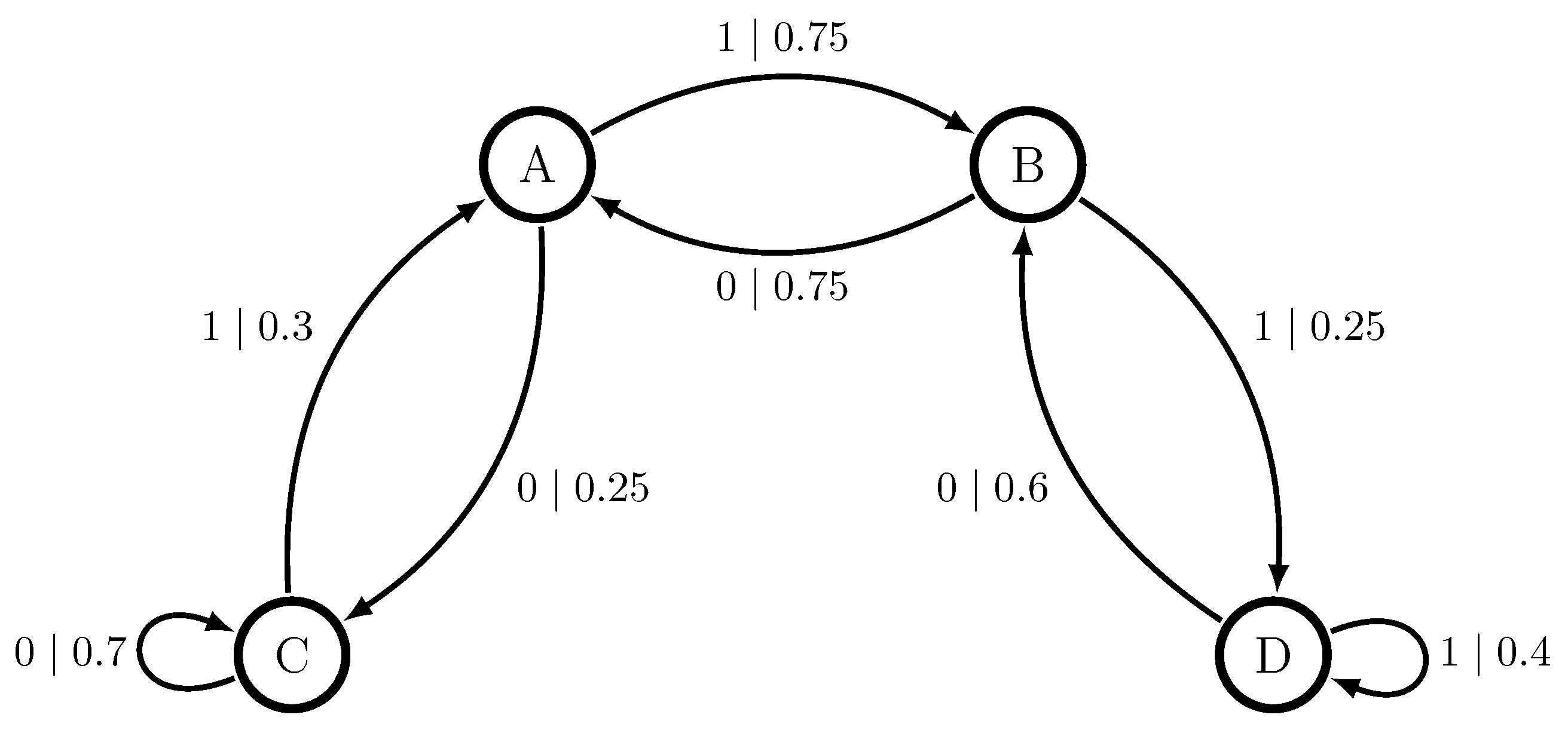
Speaking simply, a hidden Markov chain $(\Xi ,\mathcal{A},\mathcal{T})$ is a semiautomaton whose deterministic symbol-labeled transitions $\mathcal{M}=\{M_0,M_1,\dots ,M_{(n-1)}\}$ are replaced by symbol-labeled transition probabilities $\mathcal{T}=\{T^0,T^1,\dots ,T^{(n-1)}\}$, where $T_{\xi ,{\xi }^{\prime }}^a$ is the probability of transitioning from state $\xi$ to ${\xi }^{\prime }$ on the symbol $a\in \mathcal{A}$.

Paralleling the topological setting, the canonical stochastic machine presentation is a hidden Markov chain whose internal states $\Xi$—the predictive or causal states—are the equivalence classes of Equation (2)’s causal equivalence relation. The symbol-labeled transitions are then defined through the one-step conditional distributions $Pr(X^1=a|\overleftarrow{X}={\overleftarrow{x}}_i)$. For a given causal state $\xi$, we write $Pr(\overrightarrow{X}|\overleftarrow{X}\in \xi )$ since by definition each past ${\overleftarrow{x}}_i$ in the equivalence class $\xi ={[{\overleftarrow{x}}_i]}_{ϵ}$ has the same predictive distribution.

The transition probability $T_{\xi ,{\xi }^{\prime }}^a$ is then given as $Pr(X^1=a|\overleftarrow{X}={\overleftarrow{x}}_i\in \xi )$, with ${\xi }^{\prime }={[{\overleftarrow{x}}_{i}a]}_{ϵ}$, where ${\overleftarrow{x}}_{i}a$ is the new past given by concatenating the observed symbol a onto the current past ${\overleftarrow{x}}_i$. This follows from unifilarity [22]: in the stochastic setting for each internal state $\xi \in \Xi$ and symbol $a\in \mathcal{A}$ there is at most one internal state ${\xi }^{\prime }$ such that $T_{\xi ,{\xi }^{\prime }}^a>0$. It then follows that ${[{\overleftarrow{x}}_{i}a]}_{ϵ}$ is the same for all ${\overleftarrow{x}}_i\in \xi$.

Historically, the canonical stochastic machine presentation $(\Xi ,\mathcal{A},\mathcal{T})$ is known as the ϵ-machine [22] of the associated stochastic process. As described shortly, the $ϵ$-machine is a generator of its associated statistical field theory. It generates all words with their corresponding probabilities. Similar to its topological counterpart, unifilarity additionally elevates the $ϵ$-machine to a predictive presentation. Prediction in the stochastic setting means identifying the predictive distribution associated with a given past. Additionally, by definition, an $ϵ$-machine’s causal states carry unique predictive distributions.

Summing over all symbol-labeled transitions produces a Markov transition operator over the internal causal states: $T_{ϵ}={\sum }_{a\in \mathcal{A}}{T}^a$. This operator evolves probability distributions over the causal states, regardless of the symbols involved, and specifies an order-1 Markov process over the states [22]. The left eigenvector of $T_{ϵ}$ with unit eigenvalue provides the stationary distribution over causal states: $\pi T_{ϵ}=\pi$. For ergodic systems, as we consider here, $\pi$ is unique.

We emphasize that the causal states identify a hidden, internal Markov process underlying the non-Markovian process over the symbols in $\mathcal{A}$, specified by a sofic measure on a sofic shift. This inverts the abstract definition of sofic measures, given as factor maps on Markov processes [42]. There, a shift-invariant measure obeying Kolmogorov extension on a subshift of finite type produces a Markov chain of finite order and sofic shifts are abstractly defined as factor maps of subshifts of finite type. Hidden Markov chains are then given as the pushforward of the Markov measure along the factor map. Here, in contrast, we start with a statistical field theory supported on a sofic shift. The causal equivalence relation then identifies the underlying causal states and the Markov process defined over them.

With our given assumption of a stationary ergodic process over symbols we can use the stationary distribution $\pi$ and the symbol-labeled transition operators to directly extract the word probabilities $Pr\left(w\right)=\mu \left(C_0\left(w\right)\right)$ from the $ϵ$-machine presentation. First, single-symbol probabilities are given as:

$$\begin{array}{c}\hfill Pr\left(a\right)=\sum _{\xi \in \Xi }\pi \left(\xi \right)\sum _{{\xi }^{\prime }\in \Xi }{T}_{\xi {\xi }^{\prime }}^a.\end{array}$$

(3)

where ${\sum }_{{\xi }^{\prime }}{T}_{\xi {\xi }^{\prime }}^a$ gives the probability of observing the symbol $a\in \mathcal{A}$, conditioned on being in causal state $\xi$, and this is summed over all states in $\Xi$ weighted by their stationary probabilities $\pi$. We write this compactly as:

$$\begin{array}{c}\hfill Pr\left(a\right)=\langle \pi \left|T^a\right|\mathbf{1}\rangle ,\end{array}$$

(4)

where $\langle \pi |$ indicates $\pi$ as a row vector and $|\mathbf{1}\rangle$ is the column vector of all 1s.

The probability of a word $w=a_0{a}_1\dots a_k$ is then:

$$\begin{array}{cc}\hfill Pr(a_0{a}_1\cdots a_k)& =\mu \left(C_0(a_0{a}_1\dots a_k)\right)\hfill \\ \hfill & =\langle \pi |T^{a_0}{T}^{a_1}\cdots T^{a_k}|\mathbf{1}\rangle .\hfill \end{array}$$

(5)

Recall that in the topological case, the semigroup algebra of the canonical machine presentation is given through composition of the mappings $\mathcal{M}=\left\{M_a\right\}$. Now, we see the same semigroup algebraic structure in the products of the symbol-labeled transition matrices $\mathcal{T}=\left\{T^a\right\}$. In fact, the topological structure, the set of mappings $\mathcal{M}$, is recovered from the statistical structure, the set of transitions $\mathcal{T}$, by setting all nonzero elements of each $T^a\in \mathcal{T}$ to unity and then applying future equivalence.

It must be emphasized that this last step, applying future equivalence, is essential. There may be distinct $ϵ$-machines—presentations of statistical patterns—that are supported on the same sofic shift—topological pattern. Said another way, statistical patterns signify distinct structure supported on topological patterns. They are not merely “adding probabilities onto” topological patterns. Formally, the symbol-labeled transition matrices $\mathcal{T}$ can represent a different semigroup than that represented by their topological counterparts $\mathcal{M}$ on which they are supported. Appendix B illustrates this distinction.

Let us briefly turn to mention the quantitative benefits of having these presentations. Using the word probabilities as just described, in addition to the underlying pattern of the sofic shift that supports the ensemble, a wide range of statistical properties of the sequence ensembles, such as correlation functions, power spectral densities, and informational properties [45,46] can be directly determined via the $ϵ$-machine. For example, the Shannon entropy rate $h_{\mu }$ of an ensemble measures its degree of randomness and can be calculated as:

$$\begin{array}{cc}\hfill h_{\mu }& =\underset{\ell \to \infty }{lim}\frac{\mathrm{H}\left[X_{0:\ell }\right]}{\ell }\hfill \\ \hfill & =\underset{\ell \to \infty }{lim}\mathrm{H}\left[X_0\right|X_{-\ell :0}]\hfill \\ \hfill & =-\sum _{\xi \in \Xi }\pi \left(\xi \right)\sum _{a\in \mathcal{A}}\sum _{{\xi }^{\prime }\in \Xi }{T}_{\xi {\xi }^{\prime }}^{\left(a\right)}{log}_2{T}_{\xi {\xi }^{\prime }}^{\left(a\right)},\hfill \end{array}$$

where $X_{0:\ell }$ for $\ell >0$ is the random variable for the subsequence of symbols $x_0{x}_1\cdots x_{\ell -1}$. Moreover, the Shannon information in the causal states measures a process’ historical memory [47]. This is the amount of memory about the past that must be stored in order to optimally predict the future of the process.

3. Patterns in Spacetime

The preceding demonstrated that sofic shifts and their semiautomaton presentations provide a formulation of patterns in discrete one-dimensional systems. Additionally, it showed how they generalize to stochastic ensembles with associated information-theoretic measures. With this, one can argue that the theory of one-dimensional patterns in discrete stationary processes, augmented with the cited extensions, is largely complete. Now, we turn to the question of how to capture patterns in higher dimensions. While patterns in this new setting are amenable to similar analysis, there are key differences, new phenomena, and open problems.

Consider now the time evolution of symbols $\mathcal{A}$ on the sites of a spatial lattice $\mathcal{L}$. A spacetime field ${\mathbf{x}}_{}^{}\in {\mathcal{A}}^{\mathcal{L}\otimes \mathbb{Z}}$ is a time series $x_0,x_1,\dots$ of spatial configurations $x_t\in {\mathcal{A}}^{\mathcal{L}}$. With a d-dimensional lattice $\mathcal{L}={\mathbb{Z}}^d$ a spacetime field ${\mathbf{x}}_{}^{}$ is an element of a spacetime shift space ${\mathcal{A}}^{{\mathbb{Z}}^{d+1}}$ [19,21]. In what follows, upper indices on field values are spatial coordinates (e.g., at time t site i has value $x^i$) and lower indices are time coordinates (e.g., $x_t$).

Multidimensional shift spaces are notoriously difficult to study, with many simple properties being uncomputable [21,48]. Similarly, while sofic shifts and their canonical machine presentations provide a mathematical formalism for patterns as generalized symmetries in one dimension, generalizing to higher dimensions is not straightforward. Significantly, there is not a unique generalization for finite-state machines and regular languages in higher dimensions [20]. If there were a unique generalization, we could use the semiautomata special case as the mathematical representation of high-dimensional patterns.

As we argued, models that create a compressed representation of a system’s behavior must do so by harnessing patterns—predictive regularities—in the system. Fully-discrete one-dimensional systems are ideal as there is a unique minimal presentation of the system and, in this case, that predictive presentation is the pattern. The situation is more complicated in higher dimensions. A conflict arises between useful generalized spacetime symmetries and predictive presentations that faithfully generate fields in their spacetime shift spaces.

We now outline the local spacetime generalization of predictive equivalence for constructing presentations of spacetime patterns. As with finite-state machines and regular languages, degeneracy is broken when moving to higher dimensions as the spacetime generalization is not unique. In particular, we demonstrate that the shape of local “futures” determines the algebraic properties of the resulting local presentation.

3.1. Local Spacetime Presentations

Since an evolving spacetime field is a time series of spatial lattice configurations, it can be interpreted as a one-dimensional shift space over an exponentially-large alphabet (of lattice configurations). While formally well defined, however, this perspective is an unwieldy basis for a mathematical formulation of patterns in spacetime. First, for space and time translation symmetries, we typically consider the idealized case of infinitely-large spatial lattices. Thus, one must work with shift spaces over an infinitely-large alphabet. Second, capturing patterns within the spatial configurations themselves means not treating an entire lattice configuration simply as a single symbol, as done with the one-dimensional framing. There is internal organization within the spatial configurations that is dynamically and structurally important.

Therefore, we take a local approach to generalizing machine presentations of spacetime shift spaces [17,49]. This is implemented by identifying equivalence classes over local pasts that have the same future set of local futures in spacetime. The latter can be either topological (sets) or statistical (predictive distributions).

Motivated by the causal restrictions of local interactions, past lightcones in spacetime are the natural choice for local pasts when building local presentations. Formally, the past lightcone ${\mathtt{L}}^{-}$ of a site $(r,t)$ in spacetime is the set of all field values ${\mathbf{x}}_{t^{\prime }}^{r^{\prime }}$ at previous times $(t^{\prime }\le t)$ that could influence ${\mathbf{x}}_t^r$ through local interactions:

$$\begin{array}{c}\hfill {\mathtt{L}}^{-}(r,t)\equiv \left\{{\mathbf{x}}_{t^{\prime }}^{r^{\prime }}:t^{\prime }\le t\mathrm{and}|r^{\prime }-r|\le c(t-t^{\prime })\right\},\end{array}$$

(6)

where c is the finite speed of information propagation in the system. We include the present field value ${\mathbf{x}}_t^r$ in $(r,t)$’s past lightcone, but not in its local future.

Due to the richness and complication of multidimensional shift spaces, the following explores only topological spacetime patterns. Paralleling the one-dimensional development, local presentations of topological spacetime patterns are defined through the local analog of the future equivalence relations:

$$\begin{array}{c}\hfill {\mathtt{L}}_i^{-}{\sim }_F{\mathtt{L}}_j^{-}\iff F\left({\mathtt{L}}_i^{-}\right)=F({\mathtt{L}}_j^{-}),\end{array}$$

(7)

where $F\left({\mathtt{L}}_i^{-}\right)=\{$Local futures co-occurring with ${\mathtt{L}}_i^{-}\}$. We define co-occurring local futures more precisely shortly, as there are alternatives.

Relation (7)’s equivalence classes determine the internal states for a local spacetime presentation. The generalization of symbol-labeled transitions between the internal states is constructed in terms of spatial ${\left[{\sigma }^s\left({\mathbf{x}}_{}^{}\right)\right]}_t^r={\mathbf{x}}_t^{r+s}$ and temporal ${\left[{\sigma }_{\tau }\left({\mathbf{x}}_{}^{}\right)\right]}_t^r={\mathbf{x}}_{t+\tau }^r$ shift operators. (Note that all space-time shift operators commute.) For a past lightcone ${\mathtt{L}}^{-}(r,t)$ at spacetime site $(r,t)$, let ${\sigma }_{\tau }^s\left({\mathtt{L}}^{-}(r,t)\right)$ denote the action of the shift operator on all of the field values in ${\mathtt{L}}^{-}(r,t)$. That is, an entire lightcone is shifted analogously to an individual spacetime site.

The right spatial transition fringe is defined as the set difference between ${\mathtt{L}}^{-}(r,t)$ and ${\sigma }^1\left({\mathtt{L}}^{-}(r,t)\right)$. This is the generalization of the “symbol” emitted during a rightwards move in one spatial dimension. Similarly, the left spatial transition fringe is defined as the set difference between ${\mathtt{L}}^{-}(r,t)$ and ${\sigma }^{-1}\left({\mathtt{L}}^{-}(r,t)\right)$, and the forward temporal transition fringe is the set difference between ${\mathtt{L}}^{-}(r,t)$ and ${\sigma }_1\left({\mathtt{L}}^{-}(r,t)\right)$ (see Figure 4 in Ref. [49]). For simplicity, we consider spacetime fields with one spatial dimension, but the generalization to higher dimensions is straightforward.

Time and space transition fringes form the appropriate alphabet to define local spacetime presentations $(\Xi ,\mathcal{A},\mathcal{M})$, with $\Xi$ the set of past lightcone equivalence classes, $\mathcal{A}$ the set of space and time transition fringes, and $\mathcal{M}$ the fringe-labeled state transitions [49]. Briefly, a site $(r,t)$ in spacetime has an associated internal state $\xi (r,t)$ that is the equivalence class of the past lightcone ${\mathtt{L}}^{-}(r,t)$. Consider the neighboring site $(r+1,t)$, which similarly has an associated internal state $\xi (r+1,t)={\left[{\mathtt{L}}^{-}(r+1,t)\right]}_F$. The right transition fringe provides the missing information to construct ${\mathtt{L}}^{-}(r+1,t)$ from ${\mathtt{L}}^{-}(r,t)$. Therefore, $\xi (r,t)$ plus a right transition fringe uniquely determines $\xi (r+1,t)$. That is, such local presentations are unifilar, and therefore have the requisite structure of predictive presentations. Recall that predictive models are also generative.

Generating words is rather straightforward for machine presentations in one dimension, markedly less so for local spacetime presentations. The fringe-labeled transitions establish local spacetime presentations $(\Xi ,\mathcal{A},\mathcal{M})$ as local generative spacetime models. Local spacetime patches, local “words”, are generated via concatenation of transition fringe “symbols”. Denote concatenations of right spatial fringes generally as ${\mathtt{V}}_r$, to signify the particular shape of the resulting spacetime patches. Similarly, let ${\mathtt{V}}_l$ be the spacetime patches resulting from concatenations of left spatial fringes and ${\mathtt{V}}_t$ the patches from forward temporal fringes.

Note that spacetime patches are more than merely collections of values from spacetime sites. The configuration and space-time relation among the values matter. This is why we refer to their shape. The ${\mathtt{V}}_r$ patches are a distinct form of local spacetime words apart from ${\mathtt{V}}_l$ and ${\mathtt{V}}_t$. Only patches of the same shape may be concatenated together to extend patches.

Let $\mathtt{V}$ be the spacetime patches resulting from the union of forward, left, and right transition fringes. Let depth denote the number of single-fringe symbols concatenated together in a particular spacetime patch word. See Figure 2.

Concatenating fringes into local spacetime patches has the same semigroup algebra structure as in the one-dimensional setting. Similarly, the semigroup algebra is captured by the local presentations through the action of the fringe-labeled transitions $\mathcal{M}$, analogous to the one-dimensional presentations $\mathcal{P}\left(\mathcal{X}\right)$. We now examine possible choices of local futures and the algebraic properties of the induced local presentations.

3.2. The Shape of Local Futures

Recall that Relation (7) did not specify local futures when defining local presentations. The future sets $F\left({\mathtt{L}}^{-}\right)$ of past lightcones there were intentionally left ambiguous to allow for possible alternatives—alternatives that arise to address several subtleties of spacetime shifts.

Prior work assumed that the natural choice for a local future is a future lightcone ${\mathtt{L}}^{+}$ [17,18,49]. The latter is defined as all field values at subsequent times that could possibly be influenced from the given spacetime site ${\mathbf{x}}_t^r$ through the local interactions:

$$\begin{array}{c}\hfill {\mathtt{L}}^{+}(r,t)\equiv \left\{{\mathbf{x}}_{t^{\prime }}^{r^{\prime }}:t^{\prime }>t\mathrm{and}|r^{\prime }-r|\le c(t^{\prime }-t)\right\}.\end{array}$$

(8)

Co-occurring past $\left({\mathtt{L}}^{-}\right)$ and future $\left({\mathtt{L}}^{+}\right)$ lightcones at spacetime point $(r_0,t_0)$ are depicted in Figure 3 for a $1+1$ dimensional spacetime field with $c=1$. Local presentations constructed as equivalence classes of past lightcones that have the same future set of future lightcones are known as local causal states.

Interestingly, the benefit of local causal-state models derives from generalized symmetries [17,18]. However, this is a spacetime symmetry distinct from the semigroup algebra of fringe concatenations. While we describe these spacetime symmetries in more detail below, we first demonstrate that such symmetries are at odds with the semigroup algebra of fringe concatenations for local causal states. That is, while employing lightcones as local futures allows one to discover useful spacetime symmetries, the resulting local machine presentation $(\Xi ,\mathcal{A},\mathcal{M})$ is not a faithful generator of the underlying spacetime shift space. Even though all local presentations possess the unifilarity property of predictive models, the more basic generative ability falls short unless the appropriate local futures are used. We again emphasize that phenomena in higher dimensions are complicated—sometimes in counterintuitive ways, as the following demonstrates.

Elementary cellular automata (ECA)—see Appendix C—produce spacetime shift spaces with nontrivial patterns and structure in their spacetime fields; e.g., domains, particles, and particle interactions [17,50]. In addition, their one-dimensional fully-discrete spatial lattices are shift spaces and so provide a link between one-dimensional shifts and $1+1$ dimensional shifts of their spacetime fields.

Following convention, denote the mapping from a past lightcone to its equivalence class or, equivalently, to its associated local (causal) state $\xi$, as $ϵ\left({\mathtt{L}}^{-}\right)={\left[{\mathtt{L}}^{-}\right]}_F=\xi$. Crucially, this provides a local pointwise mapping over any spacetime field ${\mathbf{x}}_{}^{}$. Each site $(r,t)$ has a unique past lightcone ${\mathtt{L}}^{-}$ that is then mapped to its local state via $ϵ\left({\mathtt{L}}^{-}\right)$. We use this pointwise mapping to transform a spacetime field ${\mathbf{x}}_{}^{}$ to an associated local-state field ${\mathcal{S}}_{}^{}=ϵ\left({\mathbf{x}}_{}^{}\right)$ that shares the same coordinate geometry as ${\mathbf{x}}_{}^{}$. Each site ${\mathcal{S}}_r^t$ in the local state field ${\mathcal{S}}_{}^{}$ is the local state ${\mathcal{S}}_r^t=\xi =ϵ\left({\mathtt{L}}^{-}\right)$ that is the image under the $ϵ$-map of the past lightcone ${\mathtt{L}}^{-}$ at the spacetime point ${\mathbf{x}}_t^r$.

An example spacetime field ${\mathbf{x}}_{}^{}$ from ECA Rule 90 is shown in Figure 4 consisting of black ($x_t^r=1$) and white ($x_t^r=0$) squares. The associated local causal-state field ${\mathcal{S}}_{}^{}$ is shown as the overlaid colored letters, using lightcones as local futures. In the case of Rule 90, there is a single local causal state, labeled as $\mathsf{A}$—all past lightcones are future-lightcone equivalent.

This is consistent with prior findings [17] that connect the local causal states with the canonical machine presentations of one-dimensional sofic shifts that represent invariant sets of spatial configurations for the ECA. The full 2-shift is invariant under Rule 90, meaning there are no forbidden words in the one-dimensional spatial configurations generated by Rule 90. All binary strings have pre-images under the global dynamic $\Phi$ of Rule 90. Recall that the canonical machine presentation of full shifts consists of a single internal state and, hence, we expect the single local causal-state for the spacetime fields produced by Rule 90.

Even though there are no forbidden words in Rule 90’s one-dimensional spatial configurations, there certainly are forbidden patches in its spacetime fields. In particular, note that the ECA’s local update rule $\varphi$ corresponds to a spacetime patch in the shape of a depth-1 past lightcone—the present spacetime site together with its local neighborhood one time-step in the past. Therefore, any spacetime patch of the same shape that is inconsistent with local update rule $\varphi$ is forbidden in the spacetime shift space of the ECA’s spacetime fields. For example, the following patch is allowed by Rule 90, since ${\varphi }_{90}\left(010\right)=0$:

$$\begin{array}{c}\hfill \begin{array}{ccc}0& 1& 0\\ & 0\end{array}\end{array}$$

Therefore:

$$\begin{array}{c}\hfill \begin{array}{ccc}0& 1& 0\\ & 1\end{array}\end{array}$$

is a forbidden spacetime patch in Rule 90’s spacetime shift space.

From ECA Rule 90’s single local causal-state, it is easy to see that the local causal-state machine presentation is not a consistent spacetime generator. Since there is only one state, $\mathsf{A}$, all fringe-labeled transitions occur from state $\mathsf{A}$ back to itself. Thus, all like-shaped fringe symbols that occur may be concatenated together to form spacetime patches. Figure 4 highlights three right-transition fringes. If they are concatenated in order of orange, green, magenta (left to right) they form the depth-3 ${\mathtt{V}}_r$ patch:

$$\begin{array}{c}\hfill \begin{array}{ccccc}& & 1& 1& 0\\ & 0& 1& 0& \\ 0& 1& 1& \end{array}\end{array}$$

This patch contains the spacetime word given above that is forbidden in Rule 90’s spacetime shift. In fact, the other word of the same shape in this patch is also forbidden by Rule 90:

$$\begin{array}{c}\hfill \begin{array}{ccc}1& 1& 0\\ & 0\end{array}\end{array},$$

since ${\varphi }_{90}\left(110\right)=1$.

Concatenations of left and forward fringes produce, respectively, ${\mathtt{V}}_l$ and $V_t$ spacetime patches that similarly contain words forbidden by Rule 90’s spacetime shift space, as shown algorithmically in a supplementary Jupyter Notebook [51]. Similar results for another ECA shift space, the domain of Rule 18 discussed in more detail below, are also given in a supplementary Jupyter Notebook [52]. Empirically, we found that local causal state presentations are generically not faithful generative models of their CA spacetime shift spaces.

Comparing Figure 3 with the ${\mathtt{V}}_i$ patch shapes in Figure 2, there is little to no overlap between the “futures” (lightcones in this case) used to define the equivalence classes of past lightcones and the spacetime patches generated from fringe-labeled transitions between the equivalence classes. Therefore, it is not surprising that local presentations created with future lightcones are not faithful generators of their spacetime shifts.

In one dimension, there is only one “future” that always follows from the past. When translating forward, what once was a future becomes part of the past. This is not necessarily the case for local pasts and futures in spacetime. The predictive ability of unifilar models follows from this succession of futures becoming pasts, when combined with future equivalence. As we now see, future equivalence without the successional relation between local pasts and futures yields models that, while unifilar, are not consistent spacetime generators.

Constructively, this insight points the way to creating local presentations that are faithful generators. As the future lightcones do not play a role in generating local spacetime patches, they should not be used to define past lightcone equivalence in Relation (7). Rather, we should use spacetime patch shapes—denote them ${\mathtt{V}}_i$—that are to be generated as our notion of a local future for defining future equivalence in Relation (7). Local causal states are defined using the future sets with future lightcones $F\left({\mathtt{L}}_i^{-}\right)=\left\{{\mathtt{L}}^{+}\mathrm{co}-\mathrm{occurring}\mathrm{with}{\mathtt{L}}_i^{-}\right\}$. We can alternatively define local machine presentations whose internal states are defined as equivalence classes from Relation (7) using $F\left({\mathtt{L}}_i^{-}\right)=\left\{{\mathtt{V}}_i\mathrm{co}-\mathrm{occurring}\mathrm{with}{\mathtt{L}}_i^{-}\right\}$.

Indeed, as demonstrated computationally in the supplementary Jupyter Notebook Ref. [51], using ${\mathtt{V}}_r$ shapes with $F\left({\mathtt{L}}_i^{-}\right)=\left\{{\mathtt{V}}_r\mathrm{co}-\mathrm{occurring}\mathrm{with}{\mathtt{L}}_i^{-}\right\}$ yields a local machine presentation that is a faithful generator of ${\mathtt{V}}_r$ spacetime patches. However, this presentation is not a faithful generator of ${\mathtt{V}}_l$ or ${\mathtt{V}}_t$ spacetime patches. Similar to the use of future lightcones, local presentations can only generate faithful spacetime patches in the shape used to define $F\left({\mathtt{L}}^{-}\right)$. Therefore, as also demonstrated in Ref. [51], using ${\mathtt{V}}_l$ to define $F\left({\mathtt{L}}^{-}\right)$ results in local presentations that faithfully generate ${\mathtt{V}}_l$, but not ${\mathtt{V}}_r$ nor ${\mathtt{V}}_t$. Similar for ${\mathtt{V}}_t$.

This motivates the definition of $\mathtt{V}$ in Figure 2d as the union of ${\mathtt{V}}_r$, ${\mathtt{V}}_l$, and ${\mathtt{V}}_t$. Local presentations defined using $F\left({\mathtt{L}}_i^{-}\right)=\left\{\mathtt{V}\mathrm{co}-\mathrm{occurring}\mathrm{with}{\mathtt{L}}_i^{-}\right\}$ are faithful generators of spacetime patches in all directions emanating from a seed past lightcone. As the resulting presentations are also unifilar, additionally they are consistent predictive models of local spacetime patches. These $\mathtt{V}$ presentations can thus be seen as the most natural generalization of the predictive canonical machine presentations $\mathcal{P}\left(\mathcal{X}\right)$ for one-dimensional sofic shifts. Moreover, they possess the same semigroup algebra of “symbol” (fringe) concatenation that allows the generation and prediction of arbitrarily-long “words”—arbitrarily large spacetime patches.

It is important also to note that the spacetime fields considered here are generated by deterministic cellular automata. As pointed out above, each site in spacetime is fully determined by its depth-1 past lightcone. From Figure 2d, we see that ${\mathtt{L}}^{-}\cup \mathtt{V}$ is an enlarged past lightcone. Moreover, the depth-1 past lightcone for each site in $\mathtt{V}$ is contained within ${\mathtt{L}}^{-}\cup \mathtt{V}$. Therefore, the internal states of the $\mathtt{V}$ presentations are sets of past lightcones that make the same prediction over spacetime regions that contain the full predictive information necessary to make such predictions. This is not the case for local causal states that make predictions over future lightcones, as ${\mathtt{L}}^{-}\cup {\mathtt{L}}^{+}$ regions do not contain the depth-1 past lightcones required to make local spacetime patch predictions.

That said, as the following now details, local causal-state presentations that use future lightcones to define $F\left({\mathtt{L}}^{-}\right)$ possess interesting and useful generalized spacetime symmetries that are lost when using $\mathtt{V}$ presentations.

3.3. Generalized Spacetime Symmetries

Recall from above that machine transitions in one-dimension determine the structural relations among internal states and that they are driven by the shift operator. We just saw that the analogous fringe-labeled transition structure in spacetime is similarly related to spacetime shift operators through the definition of the fringes. However, the spacetime shift operators provide structural algebraic relations among local states independent of fringe symbols and their concatenated spacetime words. This is due to the local pointwise $ϵ$-map and the resulting shared coordinate geometry between spacetime fields ${\mathbf{x}}_{}^{}$ and corresponding local state fields ${\mathcal{S}}_{}^{}=ϵ\left({\mathbf{x}}_{}^{}\right)$.

To see this, consider two space-adjacent sites in a spacetime field, ${\mathbf{x}}_t^r$ and ${\mathbf{x}}_t^{r+1}={\sigma }^1{\mathbf{x}}_t^r$. Under the $ϵ$-map, this produces ${\xi }_i={\mathcal{S}}_t^r$ and ${\xi }_j={\mathcal{S}}_t^{r+1}={\sigma }^1{\xi }_i$. As past lightcones are defined solely in terms of spacetime distances, they are equivariant under spacetime isometries. In the present setting, these are translations.

For example, if a spacetime field ${\mathbf{x}}_{}^{}$ has exact time and space translation symmetries ${\sigma }_{\tau }{\mathbf{x}}_{}^{}={\mathbf{x}}_{}^{}$ and ${\sigma }^s{\mathbf{x}}_{}^{}={\mathbf{x}}_{}^{}$, for some s and $\tau$, then the corresponding local state field ${\mathcal{S}}_{}^{}=ϵ\left({\mathbf{x}}_{}^{}\right)$ shares these symmetries: ${\sigma }_{\tau }{\mathcal{S}}_{}^{}={\mathcal{S}}_{}^{}$ and ${\sigma }^s{\mathcal{S}}_{}^{}={\mathcal{S}}_{}^{}$. This is because the spacetime shift operators act equivalently on lightcones, so that ${\sigma }^s{\mathtt{L}}_i^{-}={\mathtt{L}}_i^{-}$ and ${\sigma }_{\tau }{\mathtt{L}}_i^{-}={\mathtt{L}}_i^{-}$. Therefore, $ϵ\left({\sigma }^s{\mathtt{L}}_i^{-}\right)=ϵ\left({\mathtt{L}}_i^{-}\right)$ and $ϵ\left({\sigma }_{\tau }{\mathtt{L}}_i^{-}\right)=ϵ\left({\mathtt{L}}_i^{-}\right)$. Note that this argument is independent of which local future shape is used, as they all define a local $ϵ$-map on past lightcones.

When future lightcones specifically are used as local futures, we previously showed (i) there are spacetime fields ${\mathbf{x}}_{}^{}$ that do not have translation symmetries, but (ii) the associated local causal state field ${\mathcal{S}}_{}^{}=ϵ\left({\mathbf{x}}_{}^{}\right)$ does [17]. These are the spacetime generalizations of partial and hidden symmetries; cf. Figure 1.

For the cellular automata examples in Ref. [17] and shown here in Figure 5, generalized symmetries—exact, partial, and hidden—in the spacetime fields are generated by the evolution of invariant one-dimensional sofic shifts (spatial configurations) under the CA dynamic. Such spacetime regions are known as domains [17,50]. Interestingly, exact symmetry domains are generated from the evolution of exact symmetry sofic shifts. Moreover, stochastic partial symmetry domains are generated from stochastic partial symmetry sofic shifts and hidden symmetry domains from hidden symmetry shifts. Examples of each of these cases are shown in Figure 5 as the generalizations of the one-dimensional cases in Figure 1. Appendix D displays the presentations $\mathcal{P}\left(\mathcal{X}\right)$ for each sofic shift $\mathcal{X}$ used to generate the fields in Figure 5.

Exact symmetries are straightforward, as just described. There is a finite s and $\tau$ such that for every site $(r,t)$ in spacetime we have that ${\sigma }_{\tau }{\mathbf{x}}_t^r={\mathbf{x}}_t^r$ and ${\sigma }^s{\mathbf{x}}_t^r={\mathbf{x}}_t^r$. Due to the shared coordinate geometry and isometry equivariance of past lightcones, this applies for the local causal state field as well: ${\sigma }_{\tau }{\mathcal{S}}_t^r={\mathcal{S}}_t^r$ and ${\sigma }^s{\mathcal{S}}_t^r={\mathcal{S}}_t^r$. The exact symmetry field shown in Figure 5a is a sample of the domain of ECA Rule 54. As can be seen, both the spacetime fields and corresponding local state fields have a period-4 translation symmetry in both time and space.

For partial symmetries, some, but not all, of the spacetime coordinates return to themselves after fixed translation, just as in one dimension. For example, there are some sites $(r^{\ast },t^{\ast })$ such that ${\mathbf{x}}_{t^{\ast }}^{r^{\ast }+s}={\sigma }^s{\mathbf{x}}_{t^{\ast }}^{r^{\ast }}={\mathbf{x}}_{t^{\ast }}^{r^{\ast }}$, but this does not hold for all $(r,t)$. As in one-dimension, a special case of partial symmetries are stochastic symmetries that become symmetric after a wildcard substitution. For example, consider a 1+1 dimensional spacetime field with $\mathcal{A}=\{0,1\}$ such that it has a checkerboard layout with 0s on the black squares and wildcards (either 0 or 1) on the white squares. The partial (stochastic) symmetry example shown in Figure 5b is ECA Rule 18’s domain, which is a strict subset (subshift) of the 0-wildcard checkerboard shift space. We examine these two spacetime shift spaces in more detail below.

Unlike in one-dimension, hidden symmetries in higher dimensions correspond to exact symmetries in the local causal-state field for spacetime fields that themselves have no symmetries, exact or partial. The hidden symmetry spacetime fields in Figure 5c and Figure 6c are samples of ECA Rule 22’s domain and their structure is manifestly harder to detect from visual inspection.

What is most important to note here is that the observable field ${\mathbf{x}}_{}^{}$ does not have any space or time translation symmetries, exact or partial. The corresponding local causal-state field ${\mathcal{S}}_{}^{}=ϵ\left({\mathbf{x}}_{}^{}\right)$ (shown in Figure 5), though, does have symmetries that are period-4 in both time and space. Essentially, there are motifs that appear in ${\mathbf{x}}_{}^{}$—such as, the black “triangles” that occur with a local period-4 structure (e.g., 1110 in space and 1100 in time). However, in contrast to a stochastic symmetry field, there is no global symmetry that captures how these stochastic motifs occur. The global hidden symmetry is more complicated than can be revealed by simple wildcard substitutions. It is uncovered, though, by the local causal-state field.

A general spacetime pattern then is one for which the local causal-state field does not exhibit spacetime symmetries. There is still an algebraic relation among the local states from the spacetime shift operators, but they do not correspond to spacetime symmetries.

Note that the example in Figure 5d has regions that are locally symmetric in both ${\mathbf{x}}_{}^{}$ and ${\mathcal{S}}_{}^{}$. However, this symmetry is globally broken by localized defects or coherent structures [17]. Figure 5d is produced from from ECA Rule 54 evolving a random initial configuration. The local symmetry regions are instances Rule 54’s domain—the exact symmetry field shown in Figure 5a.

We emphasize that, with the exception of exact symmetries, these generalized spacetime symmetries are empirically observed only with local causal-state presentations that employ future lightcone shapes. For example, the corresponding local state fields of presentations using $\mathtt{V}$ local futures are shown in Figure 6 with the same spacetime fields as Figure 5. As expected, the exact symmetry case also has space-time translation symmetries in the local state field in (a). However, there are no space-time symmetries present in the local state fields for partial (b) or hidden (c) symmetry spacetime fields when $\mathtt{V}$ local futures are employed.

Altogether, these observations portray a somewhat unsatisfactory scenario. On the one hand, lightcone local futures and the resulting local causal-state models produce insightful and predictive generalized symmetries in spacetime. Moreover, these clearly connect to the one-dimensional sofic shifts of CA spatial configurations, as demonstrated in Ref. [17]. However, we just demonstrated that local causal-state models are unfaithful generators of their underlying CA shift spaces.

On the other hand, we also showed how to create faithful local generators using $\mathtt{V}$ future shapes. These presentations thus appear to be the most natural local generalization of the canonical machine presentations in one dimension. In this case, though, the useful spacetime generalized symmetries are lost with these generative models.

Let us now examine in more detail the trade-offs between these two local presentations by diving deeper into the case of stochastic symmetries.

4. Case Study: Stochastic Symmetries

The partial (stochastic) symmetry spacetime fields in Figure 5b and Figure 6b are generated from ECA Rule 18 evolving a string from its domain’s invariant sofic shift. Appendix D shows that these are points in the stochastic symmetry sofic shift with the form 0-$\Sigma$, where $\Sigma$ is a wildcard that can be either 0 or 1.

It is easy to see from Rule 18’s lookup table ${\varphi }_{18}$ that the wildcard locations oscillate each time step between even- and odd-indexed lattice sites. Thus, the spacetime field can be interpreted as a checkerboard pattern of fixed 0s and wildcards $\Sigma =\{0,1\}$; giving the checkerboard pattern seen in the local causal-state field shown in Figure 5b. In this way, the two local causal states can be interpreted as a “fixed” 0 state and a wildcard state. The local states of the $\mathtt{V}$ machine presentation, though, do not occur in a checkerboard pattern in Figure 6b. So, they clearly cannot be assigned such semantic labels.

While the fixed-0 and wildcard semantic labels are appealing for the two local causal states, they are also misleading. For a given spatial configuration, the fixed-0 and wildcard semantics are appropriate, as it describes the (invariant) one-dimensional sofic shift of the spatial configurations. However, it is again easy to see from the Rule 18 lookup table that the wildcard semantics can no longer be assigned to the full spacetime field. Specifically, in spacetime the local update rule ${\varphi }_{18}$ forbids certain spacetime patches of the form:

$$\begin{array}{c}\hfill \begin{array}{ccc}\Sigma & 0& \Sigma \\ & \Sigma \end{array}\end{array}$$

Therefore, the spacetime shift space of Rule 18’s domain is a proper subset (subshift) of the 0-$\Sigma$ checkerboard shift space for which all realizations of the above spacetime patch are allowed.

Figure 7 demonstrates that both the local causal states and the $\mathtt{V}$ machine presentation local states reveal a checkerboard symmetry for spacetime fields in the 0-$\Sigma$ shift space. In this case, both types of local states certainly do carry the semantics of fixed-0 and wildcard $\Sigma$ in spacetime.

What does this say then about Rule 18’s domain in the context of the alternative local-state presentations in Figure 5b and Figure 6b?

First, it is interesting and not entirely clear why the choice of lightcone local futures produces local causal states that carry the strictly-spatial semantics of fixed-0 and wildcard $\Sigma$, especially when we know the wildcard semantics do not hold in spacetime. Whatever the reason, it is key to interpreting spacetime patterns through the local causal-state fields, including identifying coherent structures as locally-broken generalized symmetries in spacetime [17].

Second, this implies that the $\mathtt{V}$ machine presentation states are a more nuanced representation of the spacetime pattern of Rule 18’s domain. From above, we know the non-fixed-0 sites cannot be strictly interpreted as wildcards in spacetime. However, we can interpret these as contextually-constrained wildcards. From the 0-$\Sigma$ patch above, the outcome of the bottom $\Sigma$ is constrained by ${\varphi }_{18}$ and the outcomes of the preceding $\Sigma$s. Propagating these constraints through space and time clearly becomes complicated very quickly. However, this is a more appropriate semantic interpretation of Rule 18’s domain. So, this seems to be to what the $\mathtt{V}$ machine states correspond. As shown in a supplementary Jupyter Notebook [53], the local state field displayed in Figure 6b is reconstructed from past lightcones of depth-8 and $\mathtt{V}$s of depth-3. This produces 767 local $\mathtt{V}$ states to (approximately) capture the spacetime pattern of Rule 18’s domain. This is in contrast to the three local causal states reconstructed with the same past and future depths. (For finite-depth past lightcones, there is a third “indeterminate” state for the all-0 past lightcone.)

Note that the fixed-0 semantics still holds in spacetime and that this is not captured by the $\mathtt{V}$ presentation states. Given that $\mathtt{V}$ machine presentations are constructed to be faithful local generators of their spacetime shift spaces, it seems there is a similar spacetime contextuality to the fixed-0 sites that is necessary for faithful local generation. The spacetime contextuality present in the $\mathtt{V}$ presentation states is absent in the local causal states. Additionally, it is the latter that reveals the spacetime symmetries observed in Figure 5.

Taken all together, the spacetime patterns of partial and hidden symmetry ECA spacetime shift spaces are exceedingly complicated. Local causal-state presentations constructed from future lightcones and the $\mathtt{V}$ machine presentations capture different aspects of these patterns. One the one hand, $\mathtt{V}$ machine presentations are faithful generators and predictors of the spacetime patterns and so capture the patterns in a more direct connection with the one-dimensional case. However, local causal states capture generalized spacetime symmetries that, in the case of ECA domain shift spaces, closely connect with the (evolution of) the one-dimensional shift spaces of the invariant spatial configurations that, in turn, possess the corresponding generalized symmetries.

5. Conclusions

There is a growing body of results that use machine presentations defined from future or predictive equivalence to discover inherent, often hidden, pattern and structure in natural and engineered systems [47]. The first half of the preceding development synthesized the arguments for sofic shifts and their machine presentations as mathematical formulations of pattern and structure. In particular, the manner in which they generalize the perfect regularity of exact symmetries and the associated group algebra has been rigorously clarified. It also connected to recent results on sofic measures and their relation to stochastic $ϵ$-machine presentations of statistical patterns supported on sofic shifts.

The development’s second half overviewed the local approach to spacetime machine presentations. We showed that the standard local causal-state approach that uses lightcones as local futures reveals useful generalized spacetime symmetries. However, this comes at a cost: it does not lead to faithful generative models of the underlying shift space. This motivated introducing an alternative local presentation model using spacetime $\mathtt{V}$ shapes as local futures. We showed that these presentations are faithful generative models and that they do not possess the same generalized spacetime symmetries of the local causal states. The seeming mutual-exclusion of multiple local presentations is emblematic of the difficulty of high-dimensional shift spaces. The novel constructions given here—in particular the generative local presentations using $\mathtt{V}$ futures—may provide new paths of inquiry for investigating the organization of these rich and challenging spaces.

One advantage of the nongenerative approach using local predictive equivalence over future lightcones is that it does not rely on a finite alphabet for labeled transitions to provide the algebraic structure among local causal states. Thus, local causal states are well-defined and can be algorithmically approximated for continuum field theories. For example, they have been used to extract coherent structures in complex fluid flows [18]. The results presented here provide a theoretical underpinning and a “physics of organization” behind these unsupervised physics-informed machine learning algorithms.