Abstract
In this article, the numerical solution of the mixed Volterra–Fredholm integro-differential equations of multi-fractional order less than or equal to one in the Caputo sense (V-FIFDEs) under the initial conditions is presented with powerful algorithms. The method is based upon the quadrature rule with the aid of finite difference approximation to Caputo derivative usage collocation points. For treatments, our technique converts the V-FIFDEs into algebraic equations with operational matrices, some of which have the symmetry property, which is simple for evaluating. Furthermore, numerical examples are presented to show the technique’s validity and usefulness as well comparisons with previous results. The majority of programs are performed using MATLAB v. 9.7.
1. Introduction
One of the most significant areas of mathematics that deals with arbitrary order integrals and derivatives is fractional calculus (FC). In recent years, the idea of FC has been successfully researched to focus on a variety of issues in physics, signal processing, engineering, bio-science, and other domains. A few examples of practical uses for fractional calculus are fluid waft, electrical networks, control theory, electromagnetic, facts, optics, capacity, diffusion, and viscoelasticity (see, for instance, [1,2,3,4,5,6,7]). Many practical issues are converted into a series of fractional differential and integral equations via mathematical modeling [8]. Numerical approaches are used to approximate the solution of integro-fractional differential equations since it is challenging to obtain the analytical solution of fractional differential equations.
Then again, integro-fractional differential equations have numerous applications in the mentioned fields, and they pique the interests of many scientists. Volterra and Fredholm integro-differential equations and mixed Volterra–Fredholm integro-differential equations are three prominent types of such equations. In this regard, as in many cases, it is very difficult to find the correct analytical solutions of fractional differential and integral equations. The approximate methods have gained importance to prevent this difficulty. Many methods evaluate the approximate solution of integro-fractional differential equations; see references [9,10,11,12,13,14,15,16,17,18,19]. In [11], the author utilized modified Navot–Simpson’s quadrature for solving second-kind Volterra integral equations of singular type. Hamasalih et al. [14] proposed a technique based on quadrature methods for numerical treatment of the most general VI-FD equations of linear type. Additionally, in [17], the author applied the finite difference method together with homotopy perturbation method for numerically solving the linear VI-D equations, and Smadpour et al. [19] used the iterative method with the aid of the midpoint quadrature formula for solving fuzzy Fredholm integral equations.
The class of equations studied in this paper is the multi-order mixed Volterra–Fredholm integro-differential equations of the fractional orders that lies in the interval :
with the initial condition .
Where , , the fractional orders and and put . Furthermore, the functions , , the denotes the continuous function for all , and is the unknown function to be determined of Equation (1). The are scalar parameters. The indicates the -Caputo fractional derivative of on and for all and .
The paper is organized as follows: Section 2 presents the necessary definitions and basic preliminaries of the FC and Lagrange interpolation with basic three techniques of quadrature rules. Section 3 is devoted to the formulation of Newton–Cots formulas: Trapezoidal, Simpson’s 1/3 and Midterm techniques for solving multi-order linear mixed IFDEs of V-F type with variable coefficients. Our results are illustrated throughout the examples in Section 4. Finally, Section 5 includes a discussion for this method.
This paper aims to apply three closed Newton–Cotes techniques with the aid of the finite difference approximation for Caputo derivative terms depending on collocation points converting to an algebraic system. It also intends to evaluate the approximate solution for the multi-order linear mixed V-FIFDEs.
2. Preliminaries
In this section, definitions of the fractional Riemann–Liouville (R-L) integrals and Caputo derivative are presented as well as their relationship and some properties. In addition, we stated some basic definitions and lemmas that are used in this paper.
2.1. Fractional Operators
Definition 1
([20]). A real valued function u defined on closed bounded interval in the space , if there exists a real number , such that , where , and it is said to be in the space if and only if is in the space , where .
Definition 2
([1,3]). The Riemann–Liouville (R-L) fractional integral operator,, of order of a function is defined as:
Hence, for all and on the closed interval , we have
and
Definition 3
([8,21]). The Caputo fractional derivative operator,, of order of a function , is defined as:
For all and , so the linear property of the Caputo derivative is formulated as:
In addition, the -fractional derivative in the Caputo sense vanishes, i.e, , for any constant .
The relationship between the integral operator of R-L () and the differential operator of Caputo () is expressed in the following terms:
is the left inverse, and not the right,
Lemma 1
([22]). The finite difference approximation for the Caputo derivative of order at specific points , where , is of the form
where .
Lemma 2
([22]). Let , , and . Then, is continuous on , and , i.e.,
Lemma 3
([8,23]). Let , , and . Then, the Caputo derivative of order α of u is formed by:
2.2. Lagrange Interpolation
A Lagrange polynomial, that interpolates a function as an algebraic polynomial of degree , at some selected nodes is denoted by (see [24])
where
The Lagrange polynomial of degree and are approximately equivalent on the interval , i.e.,
If we fix and for on the interval , the Lagrange polynomial will obtain the form
then for , we have
2.3. Closed Newton–Cots Formulas
2.3.1. Trapezoidal Rule
The trapezoidal rule is the most commonly used simple technique for the numerical integration of definite integrals. The formula is based on the linear interpolation of the positive valued function between two adjacent points and . So, if an interval is divided into N equal sub-intervals with the length , it yields that there is equally spaced nodes for each . Interpolating over all nodes , the summation of the integrated interpolations can be collected in a formula as: [25]
where , and for all .The order of this approximation is .
The above formula can be expanded, for approximating definite double integrals, by applying Formula (13) to the inner and outer integral, respectively. It can be represented as
where , , for all , for all , , and for all and . The order of this approximation is .
2.3.2. Simpson’s 1/3 Rule
Simpson’s rule is another unweighted Newton–Cotes method, which approximates the definite integrals by integrating the interpolated parabola of the function between points , and . The composed Simpson’s 1/3 rule for nodes for all with setting , and such that , can be written as [25,26,27]
where
- For odd N: , for all , and for all .
- For even N: , , for all , for all , and .
2.3.3. Midpoint Rule
The midpoint is another Newton–Cotes formula in which one or both integration endpoints are omitted from the interpolation and the integration node points. It is derived from interpolating the integrated by the constant where and are two adjacent nodes. However, for the composite formula, we define , for all , so, it takes the form [25,28]
The above techniques can be modified to use for approximating definite double integrals by setting , for all and , for all . Then
3. The Solution Method
By applying each proposed method on (1) for fractional order , we can obtain a system of linear algebraic equations that can be represented in a matrix form
then, solving the matrices Equation (19) for obtains the approximated solutions at each selected node. All matrices are defined at concerned methods.
Throughout this section, we will use the following notations:
3.1. A Numerical Method Based on the Trapezoidal Rule
By setting for all , and then applying trapezoidal Formula (14) to the integral terms of (1) at nodes , and for all and , respectively, with setting , and then using finite difference approximation for fractional order (Lemma 1) together with Lemma 2, we can write (1) as follows:
where
In addition, we assumed that
and
Simply manipulating (20) for all yields a system of N linear algebraic equations of s, where s are the approximated solutions of the system at for all . Now, we can write the results in matrix form (19), where and . The structure of each matrix used in this technique is as follows:
Firstly, we assume that
with and .
Then, we have
In addition, the elements of matrix are defined as follows:
where
Moreover, and are column matrices of order and are defined as follows:
and
where and .
3.2. The Algorithm (TV-FIFDE)
The approximate solution for the mixed Volterra–Fredholm integro-differential equations of the fractional order lies in , which is based on the trapezoidal rule and can be summarized by the following Algorithm 1:
| Algorithm 1: TV-FIFDE |
| Input: , N, a, b and the initial condition . Set: . for to N do for to N do . for to n do if then else if then . else end if end for if then else . end if for to m do for to N do , for to r do if i = 0 then . else end if end for . . end for end for end for for to do , end for for to N do for to r do if i = 0 then . else end if end for end for end for Output: |
3.3. A Numerical Method Based on the Simpson’s 1/3 Rule
By setting and applying Simpson’s 1/3 Formula (16) to the integral terms of (1) at nodes , and for all and , respectively, with setting , then, using the finite difference (Lemma 1) together with Lemma 2 and depending on the value of N, we can classify the method into the following two cases:
Case I: N is even
If r is even, then (1) becomes:
where
If r is odd, then Equation (1) takes the following form:
where
We have to repeat the process in Equations (28) and (29) until r reaches N, and then, we try to combine both equations together to construct a system of linear equations. Then, it can be written in matrix form (19), where and are the same as (24) and (26) for all . Recall that N is even in this case. In addition, is a square matrix and its construction was illustrated for all as follows:
where
Case II: N is odd
Again, by repeating the process and combining both Formulas (32) and (33), we will obtain a system of linear equations. Moreover, it can be written in matrix form (19), with the only difference being that in this case, N is odd. Furthermore, the key formulas for constructing and for all are as follows:
where
3.4. The Algorithm (SV-FIFDE)
The following Algorithm 2 outline the approximate solution for a mixed Volterra–Fredholm integro-differential equations of fractional order in based on the Simpson’s 1/3 rule:
| Algorithm 2: SV-FIFDE |
| Input: , N, a, b and the initial condition . Set: . for to N do for to N do . for to n do if then else if r = j then . else end if end for if then else . end if for to m do for to N do , for to r do if then .▹ if N is even, use relations in (30), and use relations in (34) otherwise. else ▹ if N is even, use relations in (30), and use relations in (34) otherwise. end if end for . . end for end for end for for to do , end for for to N do for to r do if i = 0 then . ▹ if N is even, use relations in (31), and use relations in (35) otherwise. else ▹ if N is even, use relations in (31), and use relations in (35) otherwise. end if end for end for end for Output: |
3.5. A Numerical Method Based on the Midpoint Rule
Set , then , with , and for all and . Then, we can write Equation (1) as
since
and
The main idea is to use midpoint rule (18) for approximating the terms that lie in the intervals and and trapezoidal rule (14) for the terms in and . Furthermore, by using relation (12) on the interval all the terms of and can be approximated as
It allows us to compute initial and final terms of for all . In addition, it is helpful for obtaining better results due to repeating the process in each step.
Finally, from relations (39)–(42) and using Lemma 1 together with Lemma 2, the main Equation (38) can be written as follows:
where
After some simple manipulation and repeating (43) for all r from 1 to N, it allows obtaining a system of N linear algebraic equations of values for . Now, we are ready to write the obtained in the matrix form (19).
Recall that . Each matrix’s structure for this method is defined as follows:
where , , and for all and . Furthermore, is defined as follows:
and will be obtained in the same way before being described in the trapezoidal and Simpson’s 1/3 methods.
3.6. The Algorithm (MV-FIFDE)
We can summarize the Midpoint rule technique for solving the mixed V-FIDEs of the -fractional orders, for , at the following Algorithm 3:
| Algorithm 3: MV-FIFDE |
| Input: , N, a, b and the initial condition . Set: . for to N do for to N do . for to n do if then else if then . else end if end for if then else . end if for to m do if then else if then else if then end if for to N do if then else if then else if then end if end for end for end for end for Output: |
4. Numerical Examples
To highlight the precision of our work, we provide various examples where the exact solution already exists. For this purpose, we have written different MATLAB codes for each method (Appendix A), which generally covers the whole procedure of solution methods. They all have been performed on a computer using MATLAB v.9.7.
Example 1.
Consider a mixed Volterra–Fredholm integro-fractional differential as:
where
with initial condition , where is the exact solution.
For this example, we set . Applying Algorithms 1, 2 and 3 and then running MATLAB program (see Appendix A.1 and Appendix A.2: Listing A5) for each method gives the approximate solution to the above equation. The results are presented in Table 1 in terms of running time and least square error (L.S.Error). The L.S.Errors for and are presented in Table 2. Additionally, Figure 1 depicts a comparison between the least square error of approximate solutions for on .

Table 1.
Numerical results for Example 1, by using Trapezoidal, Simpson’s 1/3 and Midpoint methods, with setting .
Table 2.
Numerical results for Example 1, by using Trapezoidal, Simpson’s 1/3 and Midpoint methods for .
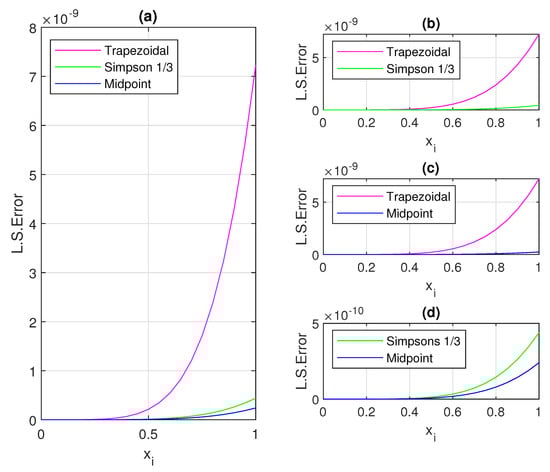
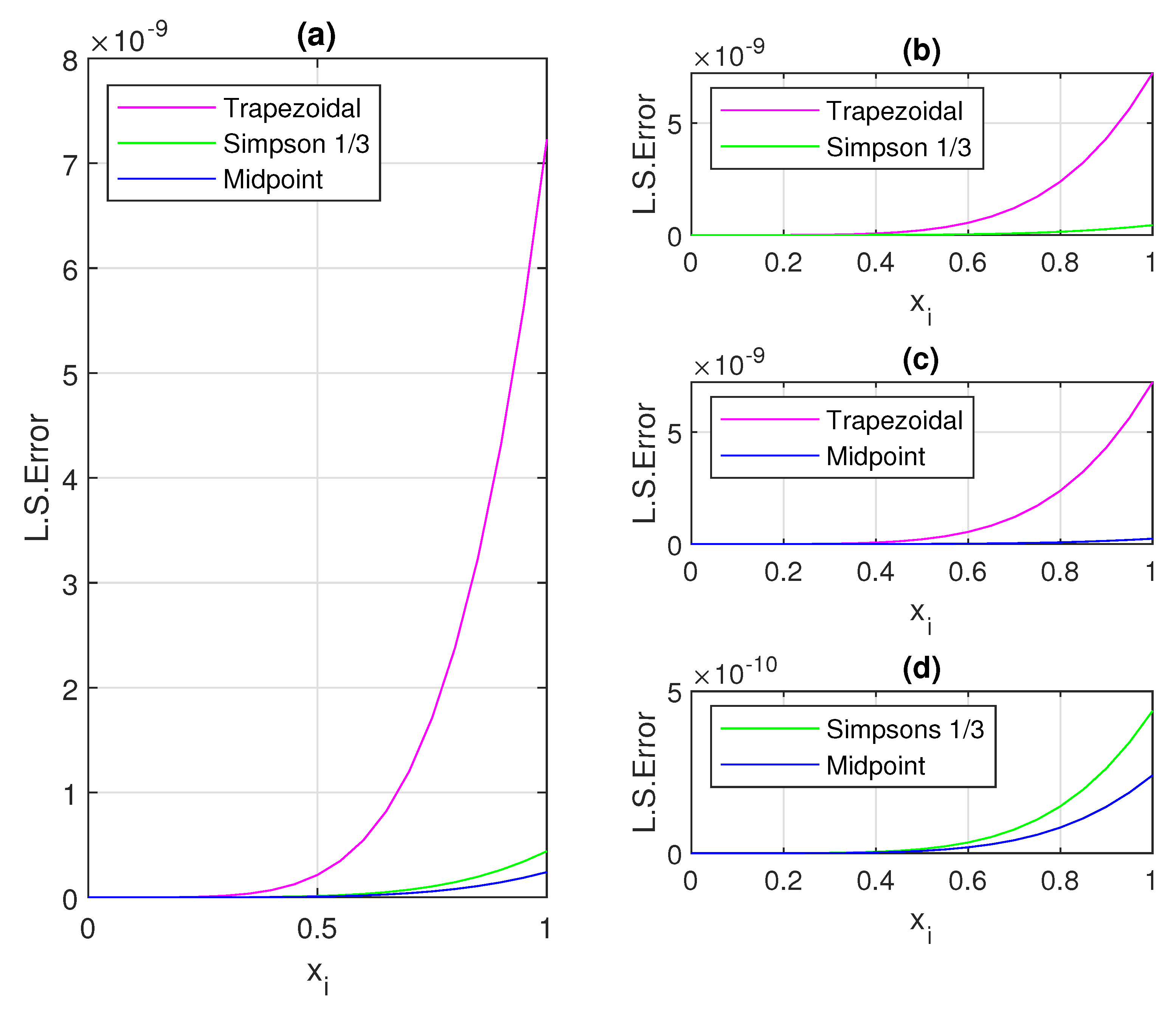
Figure 1.
(a)Least square error comparison of Trapezoidal, Simpson’s 1/3 and Midpoint methods for Example 1 with . (b) L.S.Error comparison of Trapezoidal and Simpson’s 1/3 methods. (c) L.S.Error comparison of Trapezoidal and Midpoint methods. (d) L.S.Error comparison of Simpson’s 1/3 and Midpoint methods.
Example 2.
Consider the MV-FIFDE equation on the closed bounded interval as:
where
with initial condition, , where , is the exact solution.
For the above example, numerical results are obtained by following the Algorithms 1, 2 and 3 and running the MATLAB codes (Appendix A.1 and Appendix A.2: Listing A5) that implement the steps of the algorithms. Table 3 shows the results at some selected nodes for in terms of running time and L.S.Error.
Table 3.
Numerical results for Example 2 by using Trapezoidal, Simpson’s 1/3 and Midpoint methods, with setting .
The L.S.Errors are compared in Table 4 for and 200. Additionally, Figure 2 depicts a comparison between the least square error of approximate solutions.
Table 4.
Numerical results for Example 2 by using Trapezoidal, Simpson’s 1/3 and Midpoint methods for .
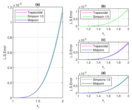
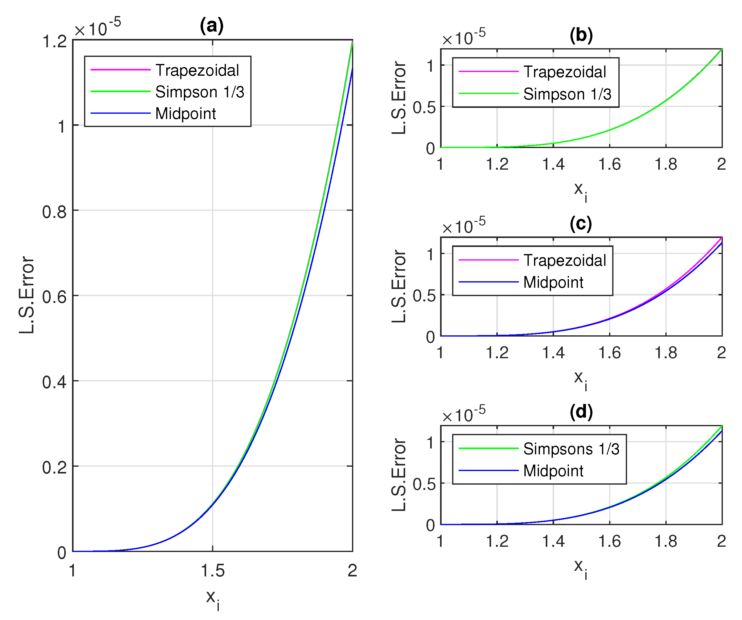
Figure 2.
(a) Least square error comparison of Trapezoidal, Simpson’s 1/3 and Midpoint methods for Example 2 with . (b) L.S.Error comparison of Trapezoidal and Simpson’s 1/3 methods. (c) L.S.Error omparison of Trapezoidal and Midpoint methods. (d) L.S.Error comparison of Simpson’s 1/3 and Midpoint methods.
Example 3.
Consider the Mixed V-FIFD equation on as:
where
with initial condition , where is the exact solution.
For the above example, numerical results are obtained by following the algorithms TV-FIFDE, SV-FIFDE and MV-FIFDE and running the MATLAB codes that implement the steps of the Algorithms 1, 2 and 3 (see Appendix A.1 and Appendix A.2). Table 5 shows the results at some selected nodes for , in terms of running time and L.S.Error.
Table 5.
Numerical results for Example 3 by using Trapezoidal, Simpson’s 1/3 and Midpoint methods with setting .
For and the L.S.Errors are compared in Table 6. Additionally, Figure 3 depicts a comparison between the least square error of approximate solutions.
Table 6.
Numerical results for Example 3 by using Trapezoidal, Simpson’s 1/3 and Midpoint methods for .
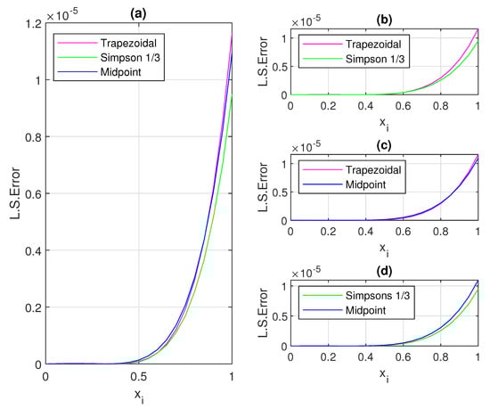
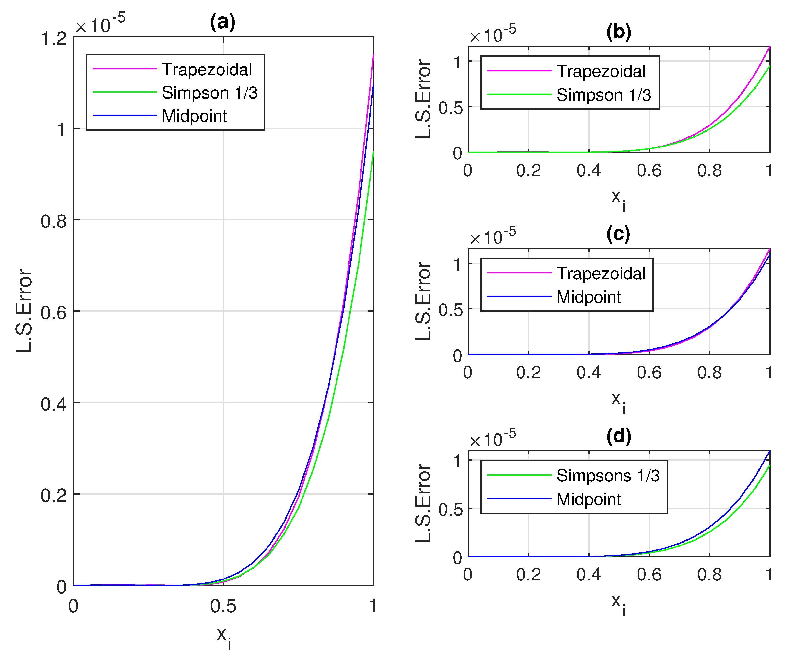
Figure 3.
(a) Least square error comparison of Trapezoidal, Simpson’s 1/3 and Midpoint methods for Example 3 with . (b) L.S.Error comparison of Trapezoidal and Simpson’s 1/3 methods. (c) L.S.Error comparison of Trapezoidal and Midpoint methods. (d) L.S.Error comparison of Simpson’s 1/3 and Midpoint methods.
5. Conclusions
We presented three numerical approaches for solving Volterra–Fredholm integro-fractional equations, and each method was described in detail. In addition, a good algorithm was created for summarizing each technique’s process. In addition, three examples are provided to test the validity and applicability of the techniques, and they are compared in terms of total least square errors and running times. In practice, we conclude with the following remarks:
- The Midpoint approach is almost more accurate than Simpson’s 1/3 and trapezoidal.
- All three techniques usually provide similar outcomes.
- The Midpoint and Simpson’s 1/3 approaches are similar, and in some cases, the Simpson’s 1/3 method gives accurate results.
- In a problem that contains Mittag–Leffler terms (see Example 3), the accuracy of the results depends on the choice N being sufficiently large (small step size h) and the number of Mittag–Leffler terms (). Due to saving time, we approximated the Mittag–Leffler into 21 terms instead of infinite terms.
- As N and are sufficiently large, the error rate decreases, and the answer approaches the exact solution.
Feature Works: The mixed Volterra–Fredholm integro-fractional differential equation studied in this article is a novel equation. We recommend using generalized Bernstein polynomials with discrete residual weighted techniques such as collocation, subdomain, moment, and least square approaches with certain adjustments. We believe they offer decent results. Additionally, it could be treated numerically by applying all quadrature techniques.
Author Contributions
Conceptualization, S.S.A. and H.A.R.; methodology, S.S.A.; software, H.A.R.; validation, S.S.A. and H.A.R.; formal analysis, S.S.A.; investigation, H.A.R.; resources, S.S.A.; data curation, H.A.R.; writing—original draft preparation, S.S.A.; writing—review and editing, H.A.R.; visualization, H.A.R.; supervision, S.S.A.; project administration, S.S.A.; funding acquisition, S.S.A. All authors have read and agreed to the published version of the manuscript.
Funding
This research received no external funding.
Institutional Review Board Statement
The study was conducted according to the guidelines of the Declaration of Helsinki and approved by the Institutional Ethics Committees of Mathematics Department, College of Basic Educations, University of Raparin, Ranya 46012, Kurdistan Region, Iraq; and Mathematics Department, College of Science, University of Sulaimani, Sulaymaniyah 46001, Kurdistan Region, Iraq.
Informed Consent Statement
Informed consent was obtained from all subjects involved in the study.
Data Availability Statement
The data used during the study are available fromthe corresponding author.
Conflicts of Interest
The authors declare no conflict of interest.
Abbreviations
The following abbreviations are used in this manuscript:
| FC | Fractional Calculus |
| VI-DE | Volterra Integro-Differential Equations |
| V-FIFDE | Mixed Volterra–Fredholm Integro-Fractional Differential Equations |
| TV-FIFDE | Trapezoidal Algorithm of Mixed V-FIFDEs |
| SV-FIFDE | Simpson’s 1/3 Algorithm of Mixed V-FIFDEs |
| MV-FIFDE | Midpoint Algorithm of Mixed V-FIFDEs |
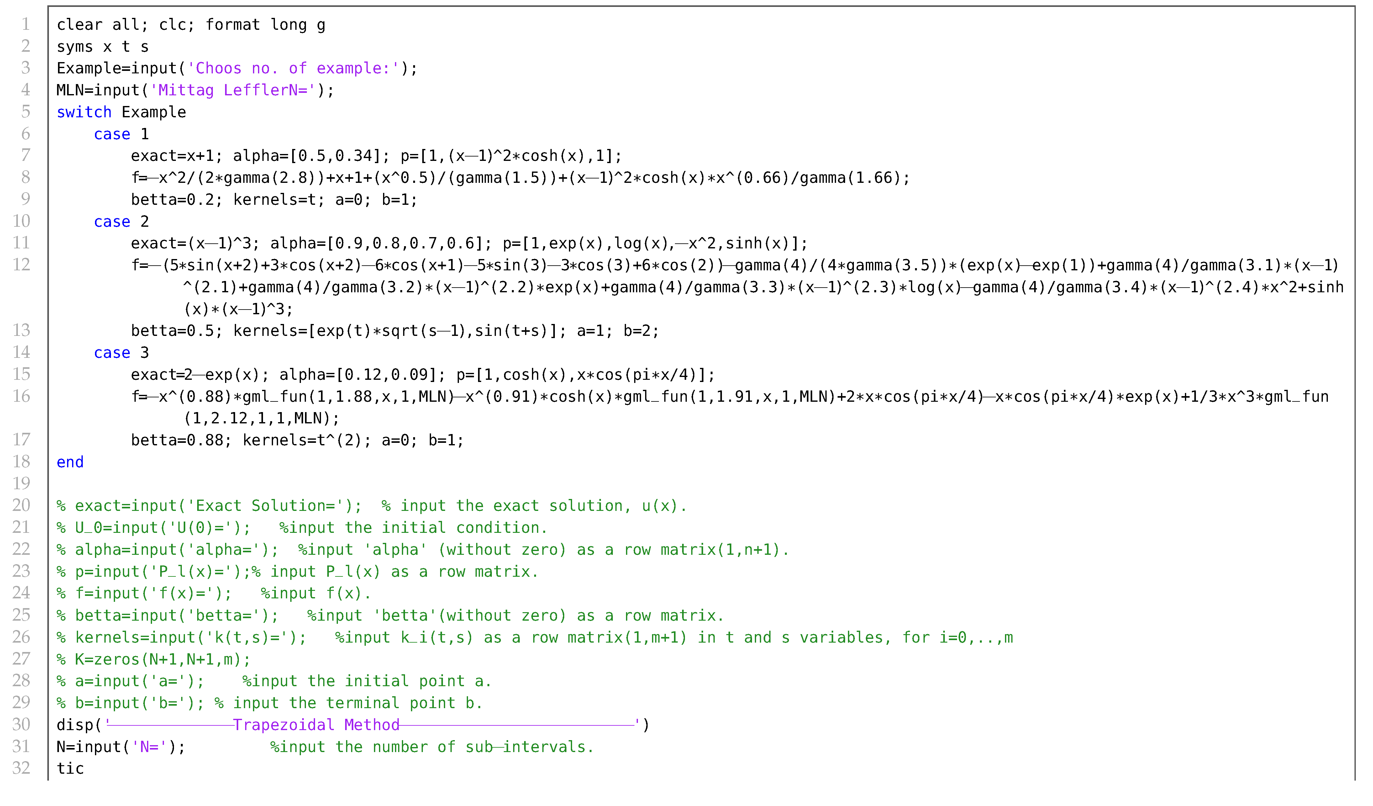
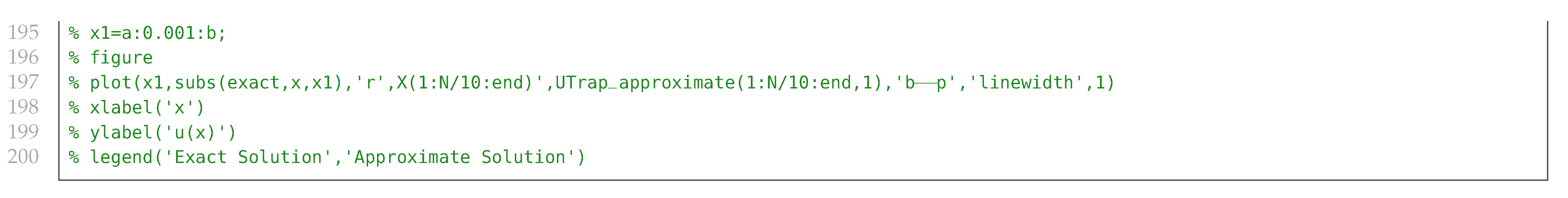
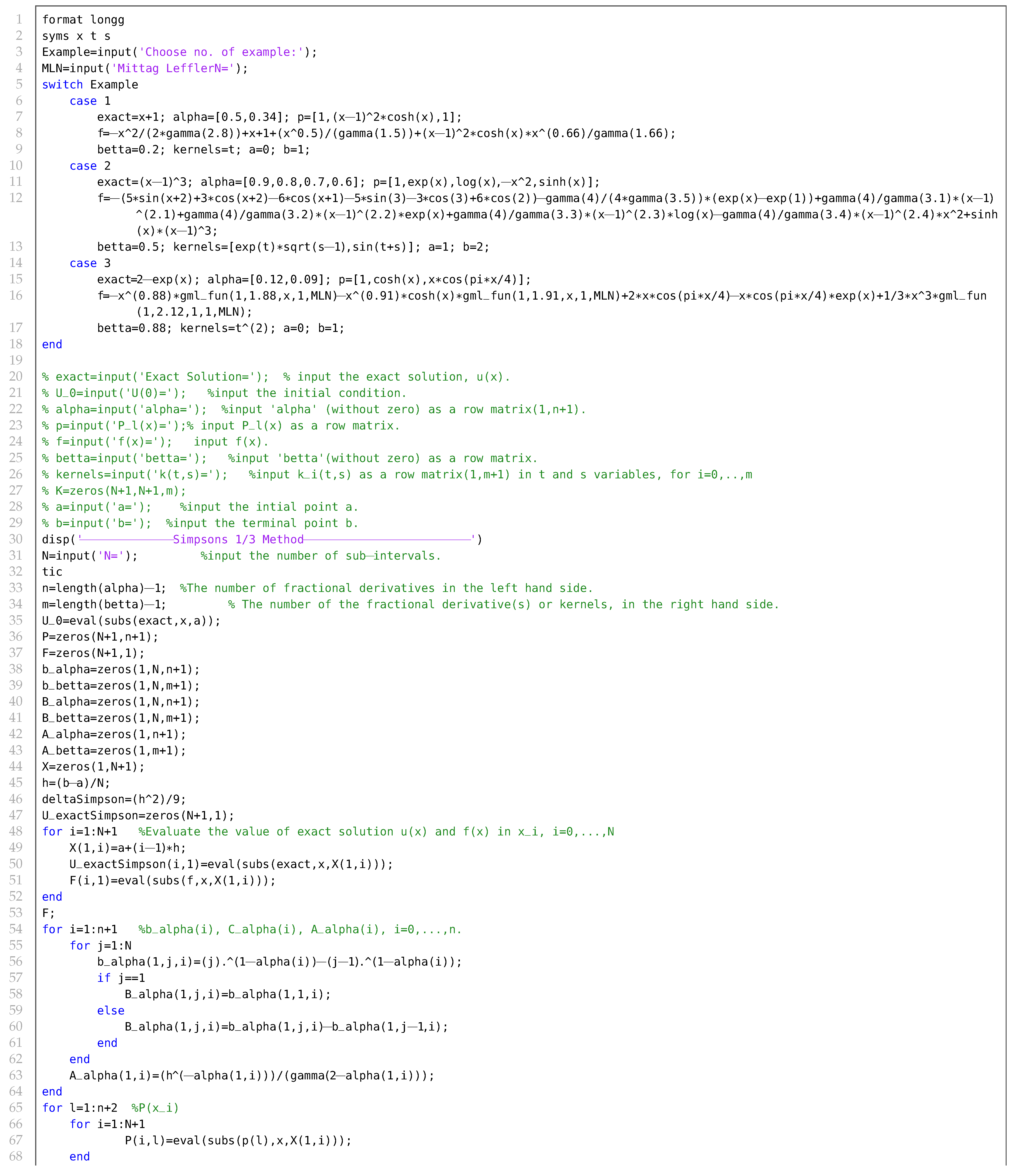
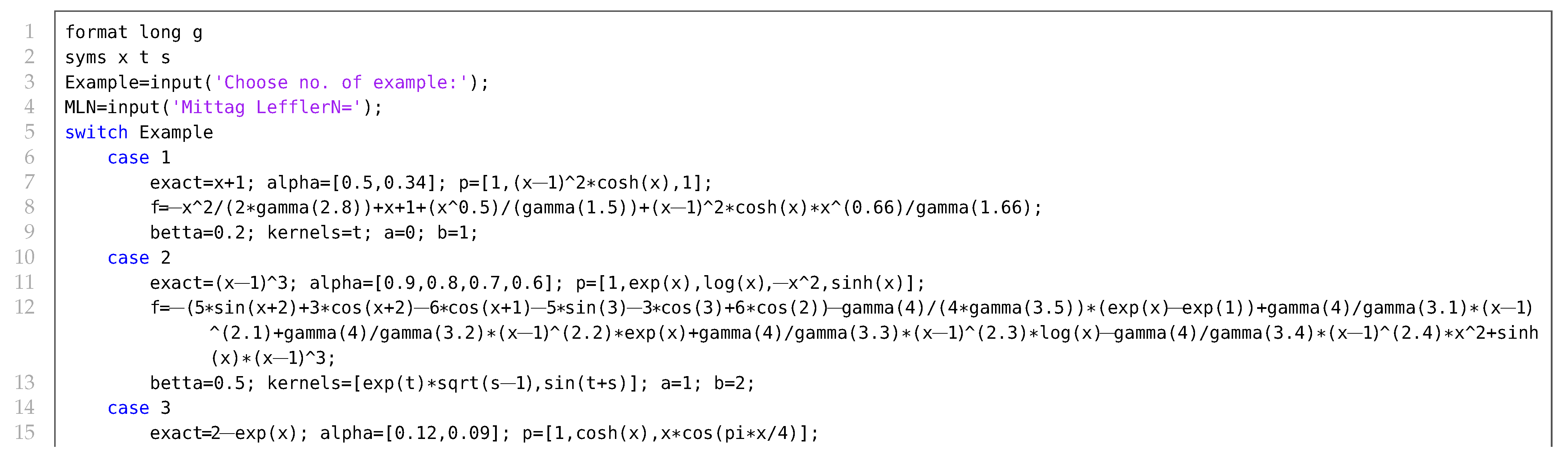
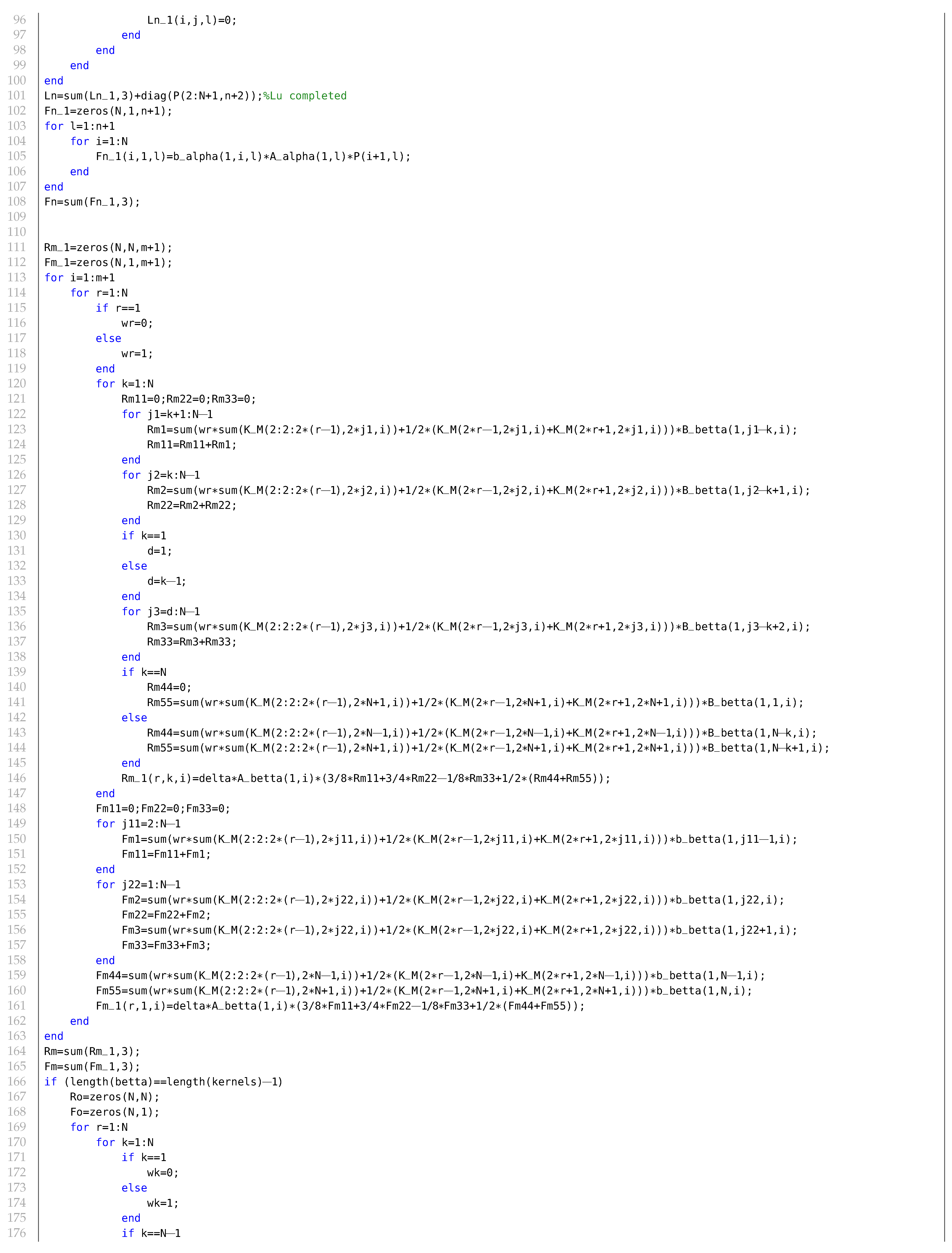
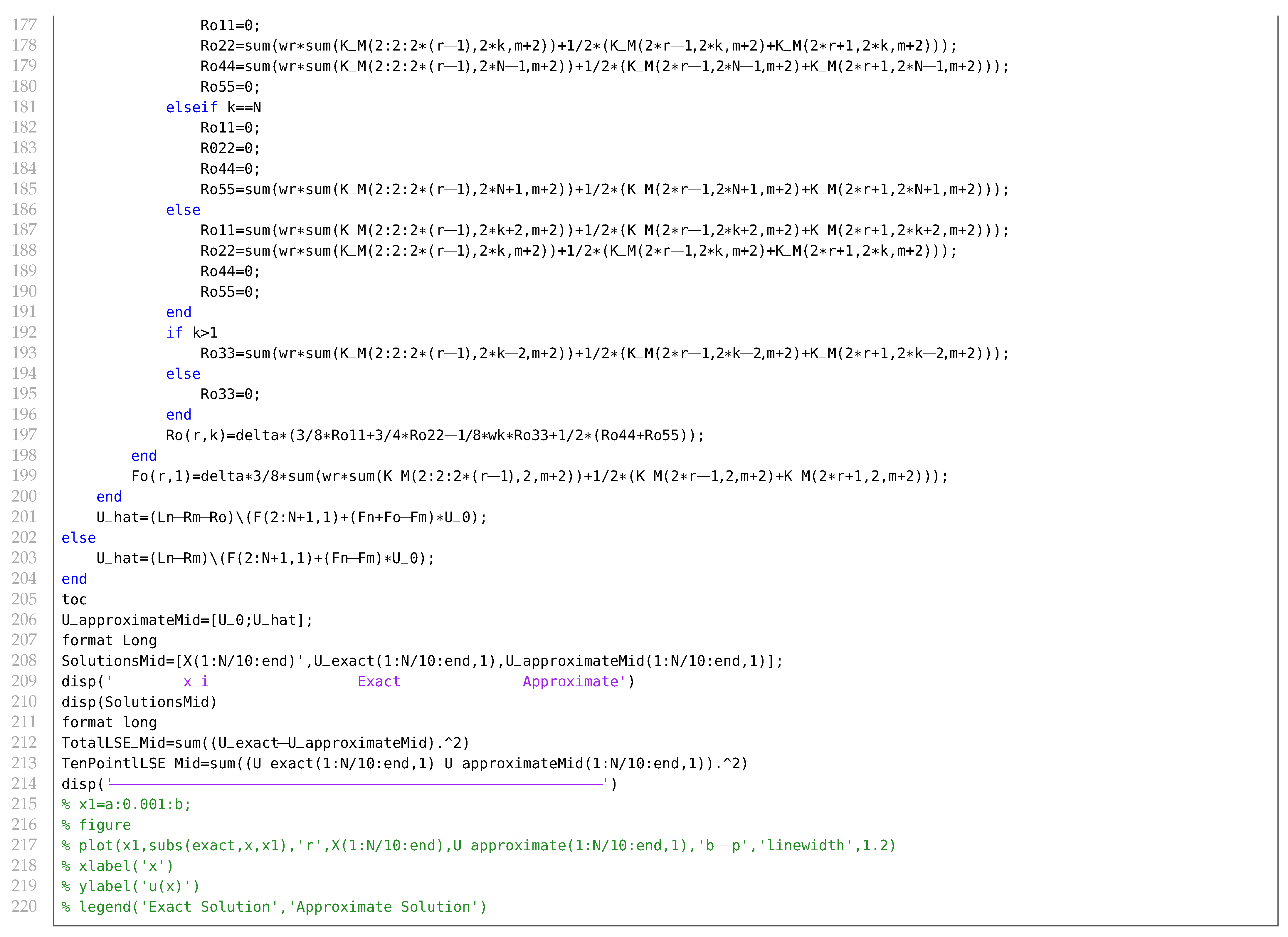
Appendix A. The MATLAB Codes
Appendix A.1. The Main MATLAB Codes
| Listing A1. Main MATLAB Code of Trapezoidal Rule. |
 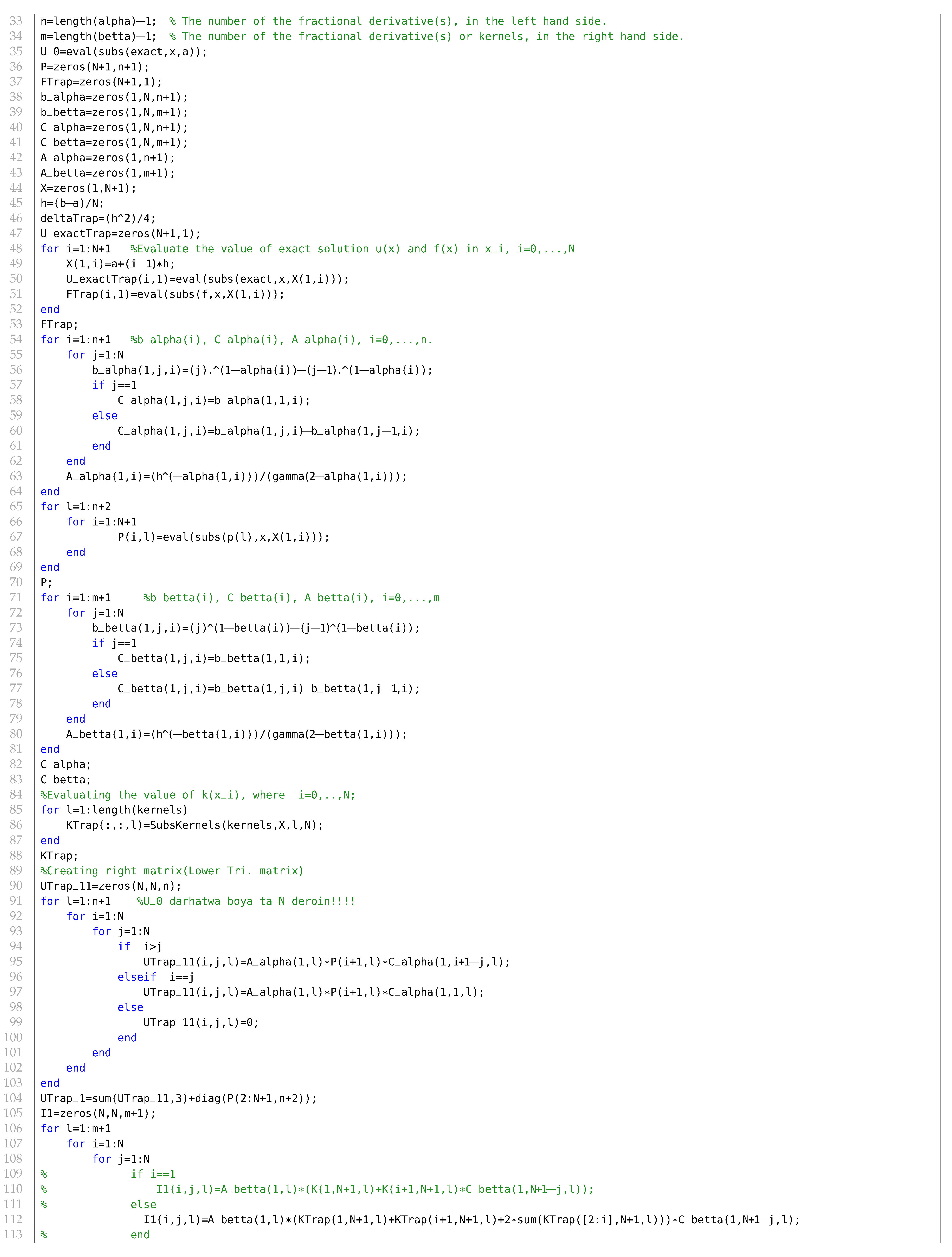 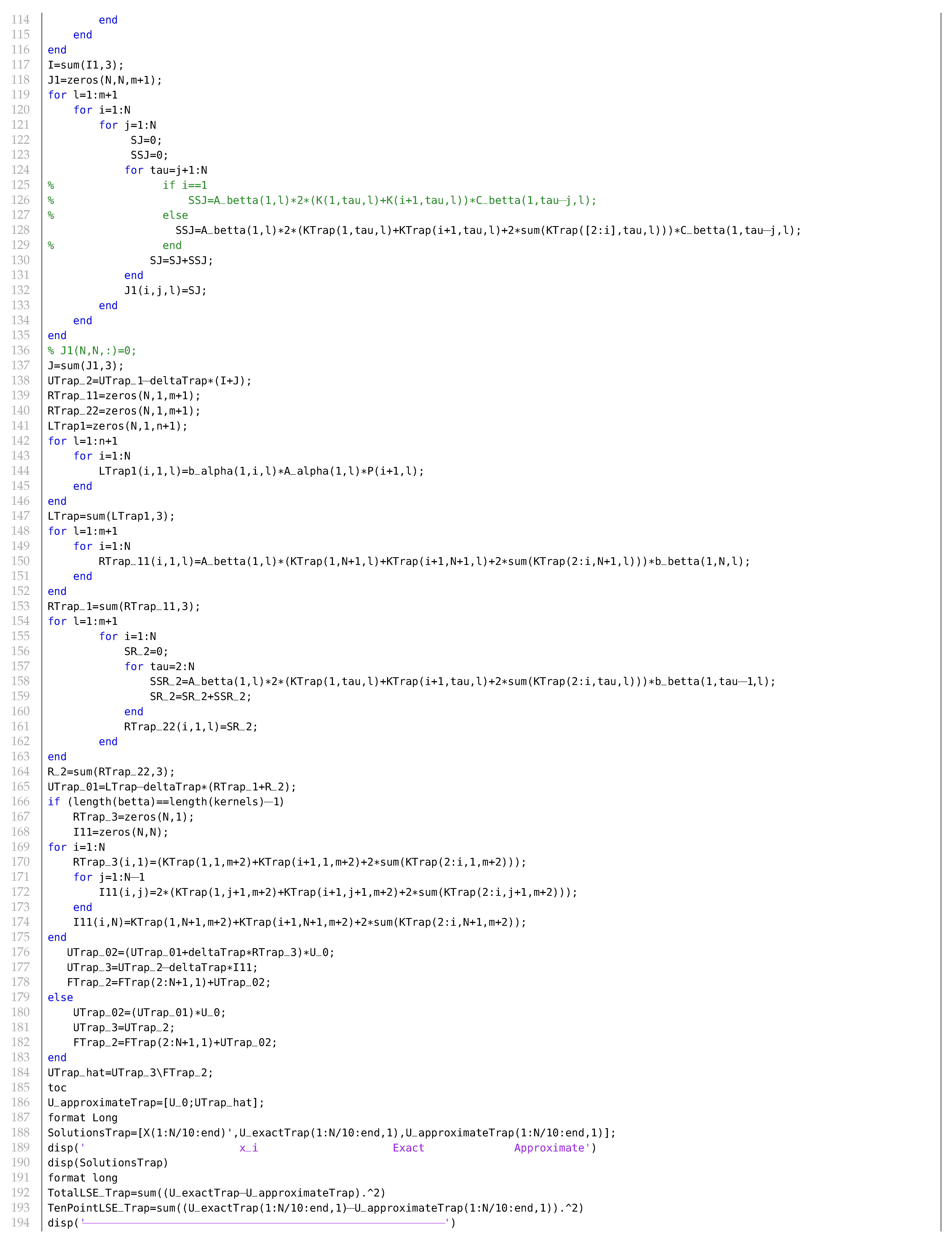  |
| Listing A2. Main MATLAB Code of Simpson’s 1/3 Rule. |
 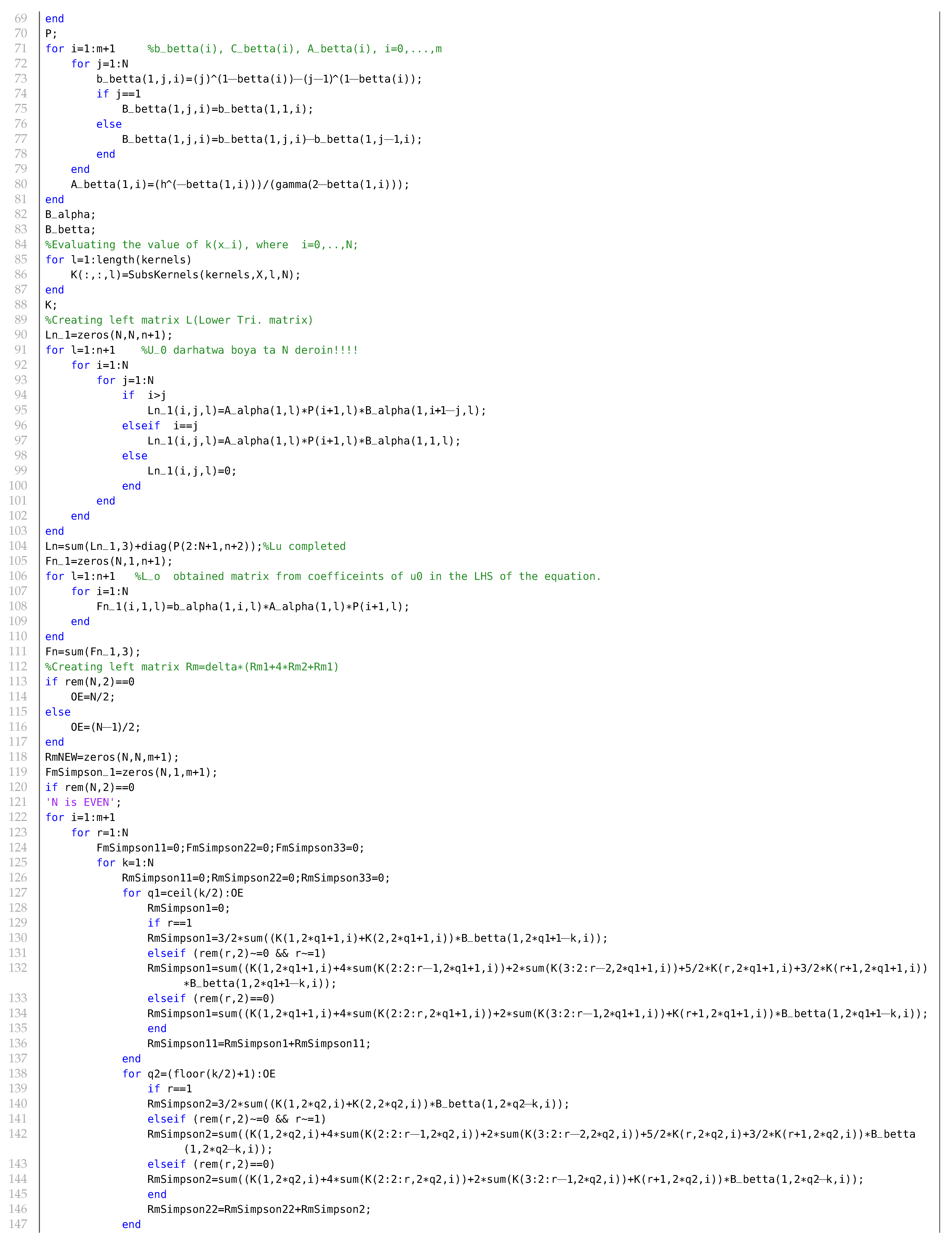 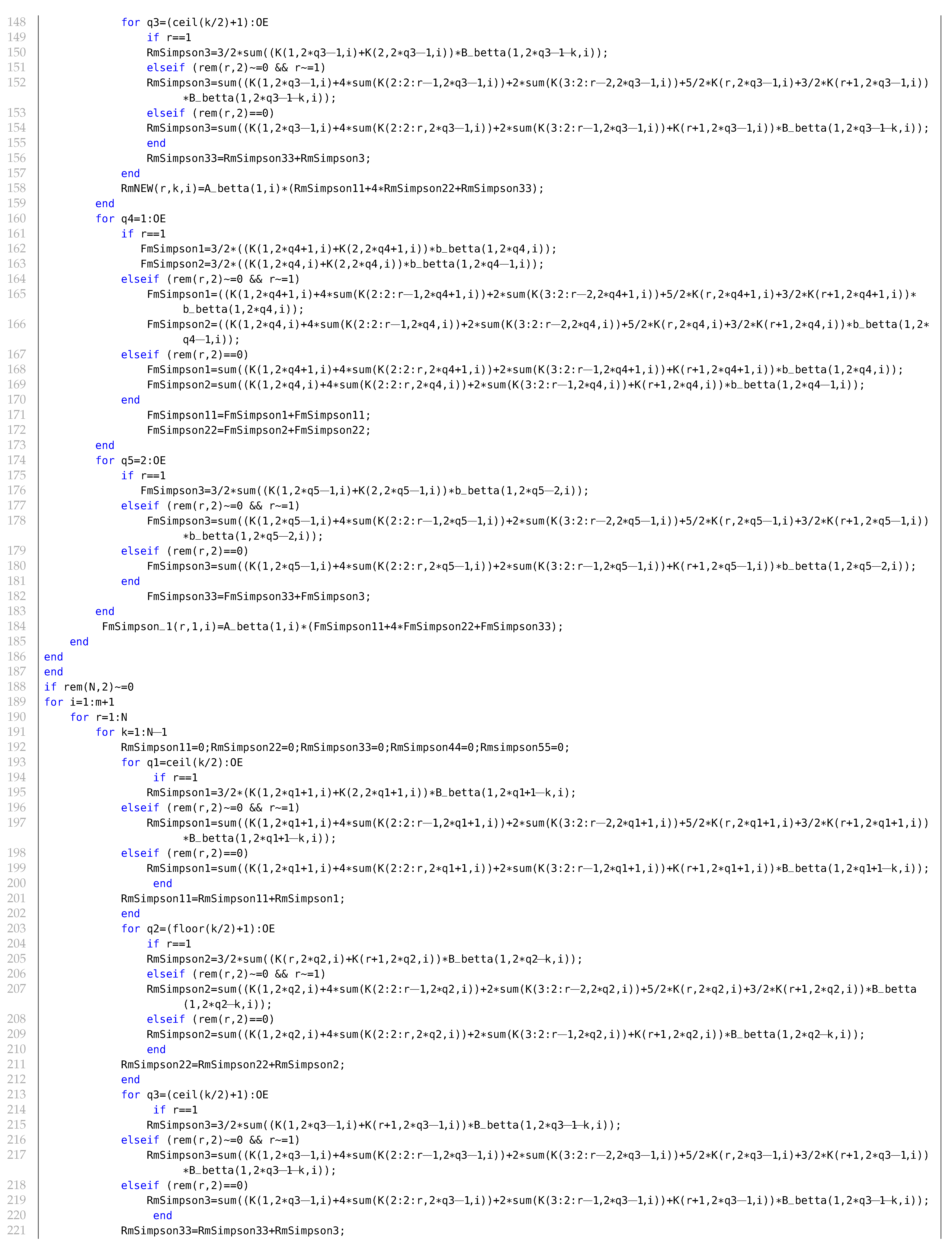 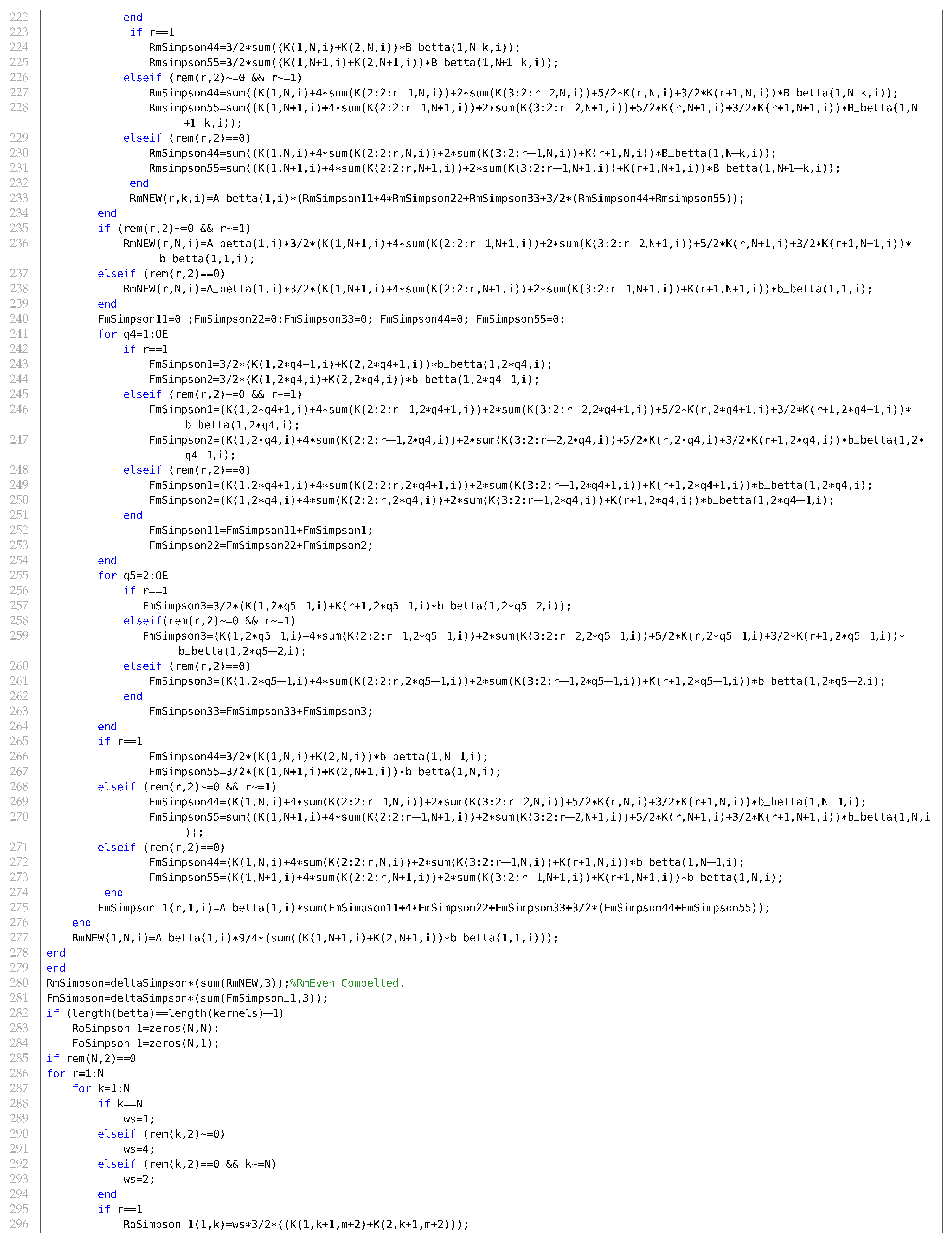 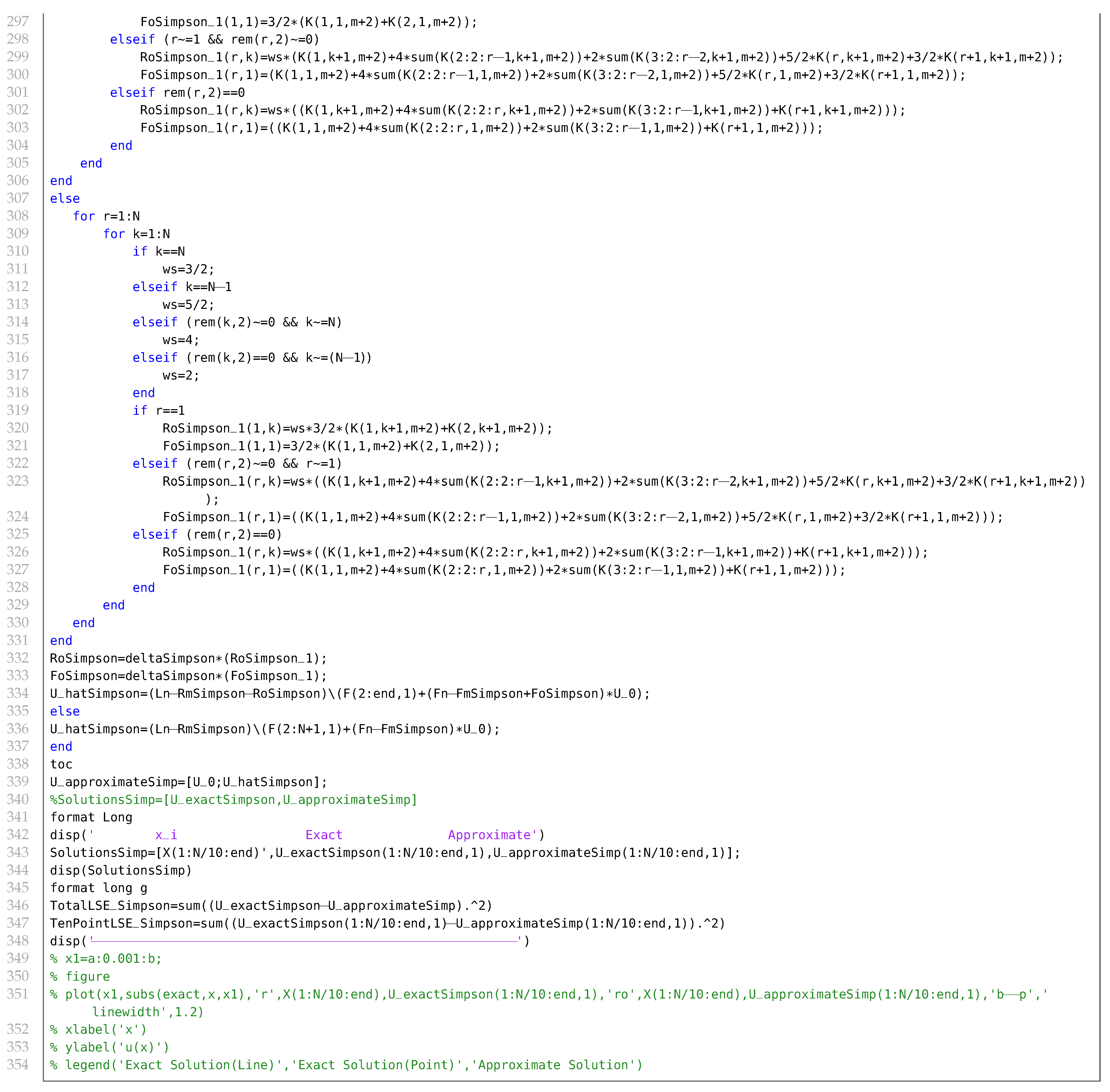 |
| Listing A3. Main MATLAB Code of Midpiont Rule. |
    |
Appendix A.2. The MATLAB Sub-Code and Functions
| Listing A4. The Mittag–Leffler Function. |
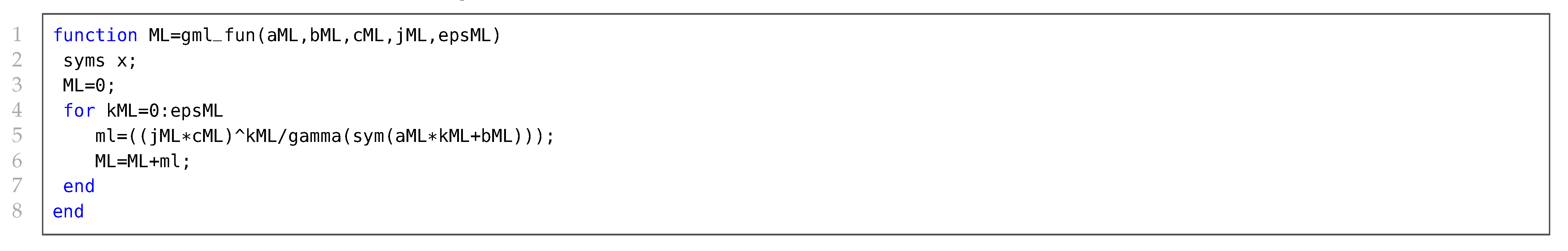 |
| Listing A5. The Kernels Substituter. |
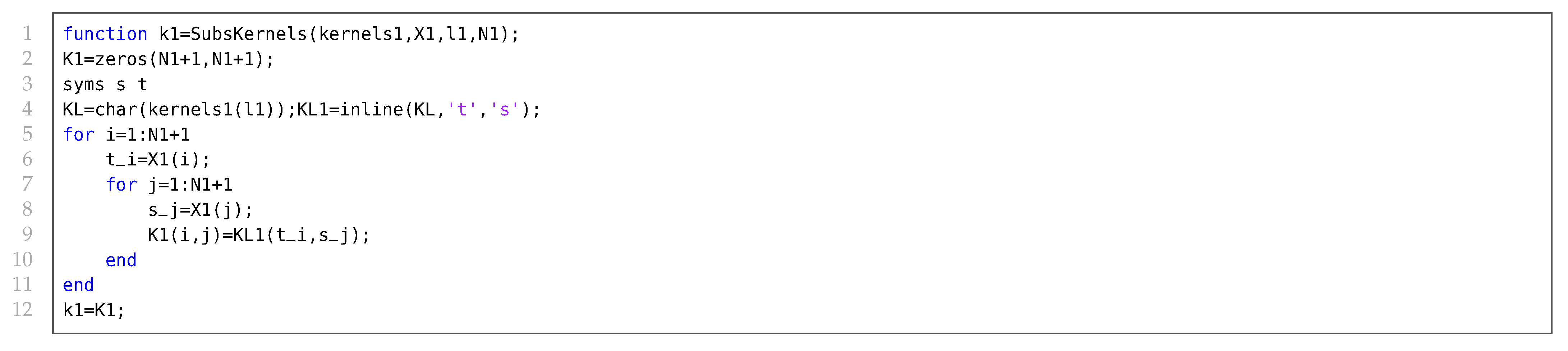 |
References
- Miller, K.S.; Ross, B. An Introduction to the Fractional Calculus and Fractional Differential Equations; Wiley: New York, NY, USA, 1993. [Google Scholar]
- Panwar, V.S.; Uduman, P.S.; Gomez-Aguilar, J.F. Mathematical modeling of coronavirus disease covid-19 dynamics using cf and abc non-singular fractional derivatives. Chaos Solitons Fractals 2011, 145, 110757. [Google Scholar] [CrossRef]
- Podlubny, I. Fractional Differential Equations: An Introduction to Fractional Derivatives, Fractional Differential Equations, to Methods of Their Solution and Some of Their Applications; Elsevier: San Diego, CA, USA, 1998. [Google Scholar]
- Ross, B. The development of fractional calculus 1695–1900. Hist. Math. 1977, 4, 75–89. [Google Scholar] [CrossRef]
- Sun, H.G.; Zhang, Y.; Baleanu, D.; Chen, W.; Chen, Y.Q. A new collection of real world applications of fractional calculus in science and engineering. Commun. Nonlinear Sci. Numer. Simul. 2018, 64, 213–231. [Google Scholar] [CrossRef]
- Tuan, N.H.; Mohammadi, H.; Rezapour, S. A mathematical model for covid-19 transmission by using the caputo fractional derivative. Chaos Solitons Fractals 2020, 140, 110107. [Google Scholar] [CrossRef]
- Valério, D.; Machado, T.J.; Kiryakova, V. Some pioneers of the applications of fractional calculus. Fract. Calc. Appl. Anal. 2014, 17, 552–578. [Google Scholar] [CrossRef]
- Roohollahi, A.; Ghazanfari, B.; Akhavan, S. Numerical solution of the mixed volterra-fredholm integro-differential multi-term equations of fractional order. J. Comput. Appl. Math. 2008, 376, 112828. [Google Scholar] [CrossRef]
- Ahmed, S.S.; MohammedFaeq, S.J. Bessel Collocation Method for Solving Fredholm–Volterra Integro-Fractional Differential Equations of Multi-High Order in the Caputo Sense. Symmetry 2021, 13, 2354. [Google Scholar] [CrossRef]
- Al-Saif, N.S.M.; Ameen, S.A. Numerical solution of mixed volterra—Fredholm integral equation using the collocation method. Baghdad Sci. J. 2020, 17, 0849. [Google Scholar]
- Araghi, M.A.F.; Hamed, D.K. Numerical solution of the second kind singular Volterra integral equations by modified Navot-Simpson’s quadrature. Int. J. Open Probl. Compt. Math. 2008, 1, 201–2013. [Google Scholar]
- Filiz, A. A fourth-order robust numerical method for integro-differential equations. Asian J. Fuzzy Appl. Math. 2013, 1, 21–33. [Google Scholar]
- Hamasalih, S.A.; Ahmed, M.R.; Ahmed, S.S. Solution Techniques Based on Adomian and Modified Adomian Decomposition for Nonlinear Integro-Fractional Differential Equations of the Volterra-Hammerstein Type. J. Univ. Babylon Pure Appl. Sci. 2020, 28, 194–216. [Google Scholar]
- Hamasalih, S.A.; Ahmed, S.S. Numerical treatment of the most general linear volterra integro-fractional differential equations with caputo derivatives by quadrature methods. J. Math. Comput. Sci. 2012, 2, 1293–1311. [Google Scholar]
- Hasan, P.M.A.; Sulaiman, N.A. Numerical treatment of mixed volterra-fredholm integral equations using trigonometric functions and laguerre polynomials. Zanco J. Pure Appl. Sci. 2018, 30, 97–106. [Google Scholar]
- Kamoh, N.M.; Gyemang, D.G.; Soomiyol, M.C. Comparing the efficiency of Simpson’s 1/3 and 3/8 rules for the numerical solution of first order Volterra integro-differential equations. Int. J. Math. Comput. Sci. 2019, 13, 136–140. [Google Scholar]
- Raftari, B. Numerical solutions of the linear volterra integro-differential equations: Homotopy perturbation method and finite difference method. World Appl. Sci. J. 2010, 9, 7–12. [Google Scholar]
- Rihan, F.A.; Doha, E.H.; Hassan, M.I.; Kamel, N.M. Numerical treatments for volterra delay integro-differential equations. Comput. Methods Appl. Math. 2009, 9, 292–318. [Google Scholar] [CrossRef]
- Samadpour, V.; Mahaleh, M.; Ezzati, R. Numerical solution of linear fuzzy fredholm integral equations of second kind using iterative method and midpoint quadrature formula. J. Intell. Fuzzy Syst. 2017, 33, 1293–1302. [Google Scholar] [CrossRef]
- Tunç, O.; Atan, Ö.; Tunç, C.; Yao, J.C. Qualitative analyses of integro-fractional differential equations with Caputo derivatives and retardations via the Lyapunov–Razumikhin method. Axioms 2021, 10, 58. [Google Scholar] [CrossRef]
- Kilbas, A.A.; Srivastava, H.M.; Juan, J.T. Theory and Applications of Fractional Differential Equations; Elsevier: Amsterdam, The Netherlands, 2006. [Google Scholar]
- Ahmed, S. On System of Linear Volterra Integro-Fractional Differential Equations. Ph.D. Thesis, University of Sulaimani, Sulaymaniyah, Iraq, July 2009. [Google Scholar]
- Ahmed, S.S.; Amin, M.B. Solving Linear Volterra Integro-Fractional Differential Equations in Caputo Sense with Constant Multi-Time Retarded Delay by Laplace Transform. Zanco J. Pure Appl. Sci. 2019, 31, 80–89. [Google Scholar]
- Dzyadyk, V.K.; Shevchuk, I.A. Theory of Uniform Approximation of Functions by Polynomials; Walter de Gruyter: Berlin, Germany, 2008. [Google Scholar]
- Burden, R.L.; Faires, J.D.; Burden, A.M. Numerical Analysis; Cengage Learning: Boston, MA, USA, 2015. [Google Scholar]
- Zahir, D.C. Numerical Solutions for the Most General Multi-Higher Fractional Order Linear Integro-Differential Equations of Fredholm Type in Caputo Sense. Master’s Thesis, University of Sulaimani, Sulaymaniyah, Iraq, March 2017. [Google Scholar]
- Hamasalih, S.A. Some Computational Methods for Solving Linear Volterra Integro-Fractional Differential Equations. Master’s Thesis, University of Sulaimani, Sulaymaniyah, Iraq, November 2011. [Google Scholar]
- Atkinson, K.E. An Introduction to Numerical Analysis; John Wiley & Sons: New York, NY, USA, 2008. [Google Scholar]
Publisher’s Note: MDPI stays neutral with regard to jurisdictional claims in published maps and institutional affiliations. |
© 2022 by the authors. Licensee MDPI, Basel, Switzerland. This article is an open access article distributed under the terms and conditions of the Creative Commons Attribution (CC BY) license (https://creativecommons.org/licenses/by/4.0/).