The Dynamics of a Fractional-Order Mathematical Model of Cancer Tumor Disease

Abstract

This article explores the application of the reduced differential transform method (RDTM) for the computational solutions of two fractional-order cancer tumor models in the Caputo sense: the model based on cancer chemotherapeutic effects which explain the relation between chemotherapeutic drugs, tumor cells, normal cells, and immune cells using a fractional partial differential equations, and the model that describes the different cases of killing rate K of cancer cells (the killing percentage of cancer cells $K$ (I) is dependent on the number of cells, (II) is a function of time only, and (III) is a function of space only). The solutions are presented using Mathematica software as a convergent power series with elegantly computed terms using the suggested technique. The proposed method gives new series form results for various values of gamma. To clarify the complexity of the models, we plot the two- and three-dimensional and contour graphics of the obtained solutions at varied values of fractional-order gamma and the selected system parameters. The solutions are analyzed with fractional and reduced differential transform methods to obtain an idea of invariance regarding the computed solution of the designed mathematical model. The obtained results demonstrate the efficiency and preciseness of the proposed method to achieve a better understanding of chemotherapy effects. It is observed that chemotherapy drugs boost immunity against the specific cancer by decreasing the number of tumor cells, and the killing rate $K$ of cancerous cells depend on the cells concentration.

1. Introduction

Tumors form following uncontrolled cell division and can be started and proliferated from one of the cells in our bodies. The tumor spreads in an unexpected way around the region where it is found, depending on whether they are malignant or benign. To destroy the diseased cells, the treatment used for this must spread quicker than the tumor movement. There are a number of treatments used to cure a cancer tumor, including surgery, chemotherapy, radiation therapy, immunotherapy, and radio frequency ablation. The choice of the treatment depends on the type of cancer and the health of the patients. The best used treatment for the cure of cancer tumor is chemotherapy. An operator splitting technique is used to tackle the system of four coupled partial differential equations which describe the interaction between malignant grown tumors and a patients’ immune system under the influence of chemotherapy treatment [1]. Chemotherapy drugs mostly infuse into a cancer area or in the blood through the vein. They are sometimes taken in the form of pills or capsules. The study of fractional calculus has drawn the attention of many scholars and medical scientists over the past few decades. Fractional calculus is being used continuously because of its applications in numerous fields, such as engineering, physical sciences, biological models, signal processing, electric circuits, anomalous diffusion, etc. Several researchers have examined the idea of fractional calculus. Bagley and Torvik [2] discussed a generalized version of Caputo’s and Scott-Blair’s fractional derivative model for the equation of motion of visco elasticity damped structures. Ishteva et al. [3] introduced new classical Laguerre functions and some of their properties are addressed using the Caputo operator of fractional calculus and Rodrigues’ fractional-order differential representation.

The mathematical models with fractional differential equations seem very helpful in explaining the growth of tumor and the interaction between tumor cells and host cells as compared to the integer order differential equations. In recent years, numerous articles related to the mathematical modelling of cancer tumor have been written. Many mathematical models have explained which components of immunity are important in the treatment of cancer. Kuznetsv and Knott [4] showed that immunotherapy does not entirely eliminate tumor cells; rather, it simply delays cancer cell renewal. Vladar and González [5] modified the model by stating that immune activity alone is insufficient to cure cancer cells; thus, therapy is also required. The tumor is not a single disease, but rather a collection of diseases with numerous similarities and significant distinctions. d’Onofrio et al. [6] presented a new mathematical model describing the interaction of tumors with the immune system and immunotherapy. Furthermore, immunotherapy’s fundamental drawback is that it is dependent on initial conditions that, in the context of medical practice, are either unknown or known with many confidence intervals. However, immunotherapy is not the only component of an anticancer therapy. The evolution of cancer immunotherapy over the last 100 years is discussed by Parish et al. [7], and it is discovered that both adaptive and innate immune systems can eliminate tumor.

Attia et al. [8] used the kernel Hilbert space method for the solution of a fractional cancer tumor model. Veeresha et al. [9] discussed the fractional model with a Caputo derivative that explains the behavior of immune cells, tumor cells, normal cells, and chemotherapy medicine. Dokuyucu et al. [10] presented the cancer tumor model, as well as the model for the Caputo-fractional operator with the uniqueness and existence of solutions of a generalized model. Arfan et al. [11] explored the mathematical tumor model with ABC fractional derivatives which described the interaction among six coupled cells, namely; tumor cells, natural killer cells, cytotoxic CD8⁺T cells, dendritic Cells, chemotherapy cells, and immunotherapy drugs cells, with six coupled partial differential equations, using a numerical method. The fourth-order Cahn–Hilliard equation in the original model was replaced with the conservative second-order Allen–Cahn equation with a space–time-dependent Lagrange multiplier proposed by Lee et al. [12]. Additionally, he utilized an operator splitting approach to solve the governing equations. Kolev and Zubik-Kowal [13] explored a novel numerical solution of various models of tissue invasion using cancerous cells, namely (I) cell-matrix interactions and cell migration, (II) the migration and proliferation of cancer cells, and (III) the production of endogenous inhibitors. They described interactions between tumor cells and the surrounding tissue, particularly the initiation of a new colony of cells and metastasis. Garrido et al. [14] examined the sequential quadratic Hamiltonian method to solve a cancerous model that was created by combining two well-known models. This model represented the differential constraint of a non-smooth optimal control problem that aims to minimize the radio and chemical dosage while reducing the volume of the tumor. Yasir et al. [15] provided an improved numerical solution of the chaotic cancer model by using the successive-over-relaxation method, and compared it against RK4 and the finite difference method. Maddalena and Ragni [16] investigated model for the evolution of a heterogeneous population of cancer stem cells and tumor cells, a nonlinear system of integro differential equations is examined and solved using the exponential Rung-Kutta method. Sabir et al. [17] considered the normal, tumor, immune, and estrogen (NTIE) compartment fractional mathematical order model and computed the numerical approach with the Levenberg–Marquardt backpropagation scheme (LMBS) combined with neural networks (NNs). LMBS-NNs, which have never been used before as the solution of the fractional breast cancer mathematical model. Ahmed et al. [18] described two generalized fractional mathematical models in the Caputo sense while considering the concentration of tumor cells for the constant killing rate.

Nonlinear fractional differential equations are used for the modelling of cancer tumor. A number of analytical and numerical methods are given in the literature for the solution of aforesaid equations. Bagheri and Khani [19] employed analytical methods, namely the direct truncation method, to obtain the solution of KDV equations. Solutions of some nonlinear fractional partial differential equations using the $\frac{G^{\prime }}{G}$ expansion method combined with fractional complex transformation have been discussed by Fan and Zhou [20]. Zhang et al. [21] coupled the homotropy perturbation method with the Laplace transform method which can reduce the computational work. This technique is also useful for various nonlinear problems such as time-fractional Fornberg–Whitham and time-fractional Fokker–Planck equations. Verma and Kumar [22] solved linear/nonlinear partial differential equations in the presence of newly proposed uniqueness and existence conditions. Rehman et al. [23] obtained the solution of the nonlinear fractional partial differential Liouville equation using the extended complex method. Khan et al. [24] discovered that the Adomian decomposition method, together with Laplace transform, is very useful for the system solution of nonlinear fractional differential equations. Singh et al. [25] implemented the fractional reduced transform method to obtain the solution of linear and nonlinear fractional differential equations.

Khlaouta and Kadem [26] combined the Shehu transform method and the reduced differential transform method to create a new analytical technique, called the modified reduced differential transform method. This modified method can be successfully implemented to solve nonlinear time-fractional wave-like equations with variable coefficients. Jaffri et al. [27] explored the reduced differential transform method to solve the linear and nonlinear PDEs on Cantor sets. Kumar and Beleanu [28] introduced a new numerical method for the Sharma–Tasso–Oliver problem and the Klein–Gordon equation of temporal fractional order with Caputo–Fabrizio (C-F) fractional derivatives. Albadarneh et al. [29] discussed a new method for approximating fractional differential equations, called the fractional finite difference method. Ali et al. [30] investigated a general form of nonlinear fractional differential equations with the linear fractional argument. The enhanced form of the Adomian decomposition method is used to solve fractional-order nonlinear differential equations proposed by Jaffri and Gejji [31]. Oyjinda and Pochai [32] described the numerical solution of an air pollution model using the finite difference technique. Bakkyaraj et al. [33] introduced Lie symmetry analysis using the Caputo-fractional derivative of the system of nonlinear fractional partial differential equations. Ibrahim et al. [34] derived a symmetry-conformable fractional derivative of complex variables. Iskenderoglu and Kaya [35] performed symmetry analysis of the initial and boundary value problem in the Caputo sense for the fractional differential equations. Yang et al. [36] discussed the numerical and analytical for the time and space symmetric fractional diffusion equation. Iyiola and Zaman [37] introduced a fractional diffusion equation model to investigate the cancer tumor. Durgess et al. [38] examined the interaction between the growth rate and diffusion coefficients with the help of a mathematical model to study gliomas. Moyo and Leach [39] investigated the application of symmetry methods to explore the mathematical model of the brain tumor. Wise et al. [40] demonstrated three-dimensional multi-species growth tumor and presented a numerical solution and analysis.

In our work, we explored two types of nonlinear fractional cancer tumor models [1] and [37] employing the reduced differential transform method (RDTM). As RDTM gives a convergent power series with elegantly computed terms which do not include linearization, discretization, perturbation, and restrictive suppositions. As a result, the number of terms of series form solutions increases as the efficiency of the solution increases. In the first model, we modified the work of Ansarizadeh et al. [1] by applying fractional order in the Caputo sense. The fractional ordinary differential equation modelling of biological systems yields more favorable results than classical integer-order modelling, which ignores memory or aftereffects manifesting in the biological system. Because of the power law form of Caputo’s kernel, namely $h_C\left(t, \beta \right)=\frac{t^{-\beta }}{\mathsf{\Gamma }\left(1-\beta \right)}, 0<\beta <1,$ the memory effects are stronger at small values of time (t). The model contains four coupled partial differential equations that explain the relation among chemotherapeutic drugs, tumor cells, normal cells, and immune cells. In the second model [37], we looked at the cancer tumor model that explains distinct cases of killing rate $K\left(x,t\right)$ of cancer cells: the killing percentage of cancer cells $K$ (I) is dependent on the number of cells and (II) is a function of time.

2. Formulation of the Problem

2.1. Models Description

Mathematical models can clarify the growth of a tumor and the interaction between tumor cells and host cells. In this work, we considered two models.

2.2. Modelling Cancer Chemotherapy Effects Using the Caputo-Fractional Derivative

This model [1] based on a system of four coupled partial differential equations explains the relations among chemotherapeutic drugs (U), tumor cells (T), normal cells (N), and immune cells (I).

$$\frac{\partial N}{\partial t}=-c_{4}TN-a_3\left(1-e^{-U}\right)N+D_N\frac{{\partial }^{2}N}{\partial x^2}+r_{2}N\left(1-b_{2}N\right),$$

(1)

$$\frac{\partial T}{\partial t}=-c_{2}IT-c_{3}TN-a2 \left(1-e^{-U}\right)T+D_T\frac{{\partial }^{2}T}{\partial x^2}+r_{1}T\left(1-b_{1}T\right),$$

(2)

$$\frac{\partial I}{\partial t}=\sigma +\left(\rho IT\beta +T\right)-c_{1}IT-d_{1}I-a_1\left(1-e^{-U}\right)I+D_I\frac{{\partial }^{2}I}{\partial x^2},$$

(3)

$$\frac{\partial U}{\partial t}=\upsilon \left(t\right)-d_{2}U+D_U \left({\partial }^{2}U\partial x^2\right).$$

(4)

where the last terms of Equations (1) and (2) represent the logistic growth rate of cells, while the capita growth and carrying capacity are represented by $r$ and $b$, respectively. $c_i$ indicates the fight of diseased cells with normal and immune cells over restricted accessible resources to survive, and these values are taken as positive. $\sigma$ represents the outside source rate for immune cells, which can be considered as constant. The immune system response in the presence of tumor cells is represented by $\frac{\rho IT}{\beta +T}$. The amount of drug over tumor area at time $t$ is denoted by $U\left(x,t\right)$. $D_N, D_T, D_I$, and $D_U$ represent the diffusion coefficients for normal cells, tumor cells, immune cells, and chemotherapeutic drugs, respectively. The parameters used in Equations (1)–(4) with acceptable range are $0.5\ge a_i\ge 0,a_2\ge a_1\ge a_3$ and $b_1\ge b_2$. The values for the immune source rate $\sigma$ lie between $0$ and $0.5$. Terms including $\left(1-e^{-U}\right)$illustrate the saturation term used for the fractional kill rate and the amount of drugs over time is represented by $\upsilon \left(t\right)$ and defined as

$$\upsilon \left(t\right)=\{\begin{array}{c}1 \left(m-1\right)\Pi <t<\left(m-1\right)\Pi +\tau \\ 0 otherwise \end{array},$$

(5)

where the interval and duration are represented by $\Pi$ and $\tau$, respectively, and $m=1, 2, 3.$ In our work, we considered the Caputo-fractional derivative of the above model. The parameters for the first model are given in the

Table 1. Selected parameter for first model [1].

Parameter	Description	Values
$a_1, a_2, a_3$	Fractional cell kill	0.2, 0.3, 0.1
$b_1, b_2$	Carrying capacity	1, 0.81
$c_1, c_2, c_3, c_4$	Competition term	1, 0.55, 0.9, 1
$d_1, d_2$	Death rate	0.2, 1
$r_1, r_2$	Per capita growth rate	1.1, 1
$\sigma$	Immune source rate	0.33
$\beta$	Immune threshold rate	0.3
$\rho$	Immune response rate	0.2
$D_N,D_T,D_I, D_U$	Diffusion coefficients	0.001, 0.001, 0.001, 0.001

below.

2.3. Modelling Cancer Tumor Based on the Cell’s Concentration

In the second model, a diffusion equation model is proposed by [38], in which a spherical-shaped tumor is considered with the growth rate $q$ and the therapy-dependent killing percentage $k$.

$$\frac{\partial v\left(x, t\right)}{\partial t}=D\frac{1}{r^2}\frac{\partial }{\partial r}\left(\frac{1}{r^2}\frac{\partial v\left(x, t\right)}{\partial r}\right)+qv\left(x,t\right)-kv\left(x,t\right).$$

(6)

where the amount of tumor cells at point $x$ and at time $t$ is represented by $v\left(x,t\right)$ and the diffusivity constant is given by $D$. The one-dimensional model for the above equation was investigated by Moyo and Leach [39] with the variable killing percentage $K\left(x,t\right)$.

$$\frac{{\partial }^{2}v\left(x,t\right)}{\partial x^2}-K\left(x,t\right)v\left(x,t\right)-\frac{\partial v\left(x, t\right)}{\partial t}=0.$$

(7)

$K\left(x,t\right)$ can be selected as a constant function of time only, or as a function of both time and position. In our work, we considered three cases of $K\left(x,t\right)$: the killing percentage of cancer cells $K$ (I) is dependent on the number of cells, (II) is a function of time only, and (III) is a function of space only.

2.4. Method Description

To explain the basic definitions of the suggested method RDTM, we consider whether the function $\omega \left(x,t\right)$ is continuously differentiable and analytic with respect to $t$, then let

$${{\omega }^{\prime }}_k\left(x\right)=\frac{1}{\mathsf{\Gamma }\left(k\gamma +1\right)}{\left[\frac{{\partial }^{k\gamma }}{\partial t^{k\gamma }}\omega \left(x,t\right)\right]}_{t=o},$$

(8)

where $\gamma$ describes the fractional derivative. Here, $\omega \left(x,t\right)$ and ${{\omega }^{\prime }}_k\left(x\right)$ represent the original function and the transform function, respectively. The inverse transform of ${{\omega }^{\prime }}_k\left(x\right)$ is defined as follows:

$$\omega \left(x,t\right)={\displaystyle \sum }_{k=0}^{\infty }{{\omega }^{\prime }}_k\left(x\right) t^{k\gamma }.$$

(9)

Upon combining Equations (8) and (9), we obtain

$$\omega \left(x,t\right)={\displaystyle \sum }_{k=0}^{\infty }\frac{1}{\mathsf{\Gamma }\left(k\gamma +1\right)}{\left[\frac{{\partial }^{k\gamma }}{\partial t^{k\gamma }}\omega \left(x,t\right)\right]}_{t=o}{t}^{k\gamma }.$$

(10)

The above definitions tell us that the results of RDTM are derived from the power series expansion. To illustrate a general idea of the reduced differential transform method, we consider the general differential equation of fractional order of the form

$$L\omega \left(x,t\right)+R\omega \left(x,t\right)+\mathrm{Ɲ}\omega \left(x,t\right)-h\left(x, t\right)=0,$$

(11)

with initial condition

$$\omega \left(x,0\right)=g\left(x\right),$$

(12)

where $\mathrm{Ɲ}$ is a non-linear operator, $R$ is a linear operator, $L=\frac{{\partial }^{k\gamma }}{\partial t^{k\gamma }}$ is a Caputo-fractional derivative, $h$ is a known function, and $v$ is an unknown function. According to the proposed method, the iterative formula will be

$$\frac{\mathsf{\Gamma }\left(k\gamma +\gamma +1\right)}{\mathsf{\Gamma }\left(k\gamma +1\right)}{{\omega }^{\prime }}_{k+1}\left(x\right)={h^{\prime }}_k\left(x\right)-R{{\omega }^{\prime }}_{k+1}\left(x\right)-\mathrm{Ɲ}{{\omega }^{\prime }}_{k+1}\left(x\right),$$

(13)

with transformed initial condition as

$${{\omega }^{\prime }}_0\left(x\right)=g\left(x\right).$$

(14)

Here, ${{\omega }^{\prime }}_k\left(x\right),{h^{\prime }}_k\left(x\right),R{{\omega }^{\prime }}_{k+1}\left(x\right)$, and $\mathrm{Ɲ}{{\omega }^{\prime }}_{k+1}\left(x\right)$ are the transform functions of $L\omega \left(x, t\right),h\left(x, t\right),R\omega \left(x, t\right)$, and $\mathrm{Ɲ}\omega \left(x, t\right)$, respectively.

By using Equation (14) into (13) alongside some iterative calculations, we obtain the following ${{\omega }^{\prime }}_k\left(x\right)$ values. Applying Equation (9) on the set of values $\left\{{{\omega }^{\prime }}_k\left(x\right), k=0, 1, 2, \dots , \infty \right\}$ now gives the approximate solution, as follows:

$$\omega \left(x,t\right)=\underset{\mathrm{n}\to \infty }{\lim }{\displaystyle \sum }_{k=0}^{\infty }{{\omega }^{\prime }}_k\left(x\right) t^{k\gamma }.$$

(15)

The basic operations [25] of the reduced differential transform method can now be determined using Equations (8) and (9).

Theorem 1. 

If the original function is$\omega \left(x,t\right)=u\left(x,t\right)\pm v\left(x,t\right)$, the transform function will be ${{\omega }^{\prime }}_k\left(x\right)={u^{\prime }}_k\left(x\right)\pm {v^{\prime }}_k\left(x\right)$.

Theorem 2. 

If the original function is$\omega \left(x,t\right)=u\left(x,t\right)v\left(x,t\right)$, the transform function will be${{\omega }^{\prime }}_k\left(x\right)={\displaystyle \sum }_{m=0}^k{u^{\prime }}_m{v^{\prime }}_{k-m}\left(x\right)={\displaystyle \sum }_{m=0}^k{v^{\prime }}_m{u^{\prime }}_{k-m}\left(x\right)$.

Theorem 3. 

If the original function is$\omega \left(x,t\right)=\frac{{\partial }^{M\beta }}{\partial x^{M\beta }} v\left(x,t\right)$, the transform function will be ${{\omega }^{\prime }}_k\left(x\right)=\frac{\mathsf{\Gamma }\left(k\beta +M\beta +1\right)}{\mathsf{\Gamma }\left(k\beta +1\right)}{v^{\prime }}_{k+M}\left(x\right)$.

Theorem 4. 

If the original function is $\omega \left(x,t\right)=x^n{t}^{m}v\left(x,t\right)$, the transform function will be${{\omega }^{\prime }}_k\left(x\right)=x^n{v^{\prime }}_{k-m}\left(x\right)$.

Theorem 5. 

If the original function is $\omega \left(x,t\right)=x^n{t}^m$, the transform function will be ${{\omega }^{\prime }}_k\left(x\right)=x^n\delta \left(k-m\right), \delta \left(k-m\right)=\left\{\begin{array}{c}1 k=m\\ 0 k\ne m\end{array}\right\}$.

Now, we will discuss the convergence of the method.

Since the RDTM is derived from a power series expansion with an initial time of zero, it is given as:

$$\omega \left(x,t\right)={\displaystyle \sum }_{k=0}^{\infty }{b}_k\left(x\right) t^{k\gamma }, t\in j.$$

(16)

where $j=\left(0, m\right), m>0.$

Now, we will look at the condition of convergence for the suggested method.

Theorem 6. 

If${\mathsf{\psi }}_k\left(x,t\right)=b_k\left(x\right) t^{k\gamma },$ then$\omega \left(x,t\right)={\displaystyle \sum }_{k=0}^{\infty }{\mathsf{\psi }}_k\left(x,t\right)$, ∀ $k\ge 0$

i.

If 0 < ξ < 1 and $\Vert {\mathsf{\psi }}_{k+1}\Vert \le \mathsf{\xi }\Vert {\mathsf{\psi }}_k\Vert ,$ then it is convergent;

ii.

If ξ > 1 and $\Vert {\mathsf{\psi }}_{k+1}\Vert \ge {\mathsf{\xi }\Vert \mathsf{\psi }}_k\Vert ,$ then it is divergent.

Proof. 

The theorem stated above is a particular case of Banach’s fixed-point theorem. We will use this theorem for evidential purposes. Let $\left(C\left[j\right],\Vert .\Vert \right)$ be the Banach space on all continuous functions on $j$ with the norm $\Vert {\mathsf{\psi }}_k\left(x,t\right)\Vert =\Vert b_k\left(x\right) t^{k\gamma }\Vert$ and $\Vert b_0\left(x\right)\Vert <M_0>0.$ Now, defining the sequence of partial sum ${\left\{{ℌ}_i\right\}}_{i=0}^{\infty }$ as:

$${ℌ}_i={\mathsf{\psi }}_0+{\mathsf{\psi }}_1+{\mathsf{\psi }}_2\dots \dots +{\mathsf{\psi }}_i.$$

(17)

We aim to prove that ${\left\{{ℌ}_i\right\}}_{i=0}^{\infty }$ is a Cauchy sequence in the Banach space. To achieve this goal, we take the following equation:

$$\Vert {ℌ}_{i+1}-{ℌ}_i\Vert =\Vert {\psi }_{i+1}\Vert \le \xi \Vert {\psi }_i\Vert \le \cdots \le {\xi }^{i+1}\Vert {\psi }_0\Vert \le {\xi }^{i+1}{M}_0.$$

(18)

Using the above equation and triangular inequality, for any $i, p\in \mathrm{N}$ with $i$ ≥ $p$, we have:

$$\begin{gathered} \Vert {ℌ}_i-{ℌ}_p\Vert =\Vert \left({ℌ}_i-{ℌ}_{i-1}\right)+\left({ℌ}_{i-1}-{ℌ}_{i-2}\right)+\cdots +\left({ℌ}_{p+1}-{ℌ}_p\right)\Vert \\ \le \Vert {ℌ}_i-{ℌ}_{i-1}\Vert +\Vert {ℌ}_{i-1}-{ℌ}_{i-2}\Vert +\cdots +\Vert {ℌ}_{p+1}-{ℌ}_p\Vert \\ \le \frac{1-{\xi }^{i-p}}{1-\xi }{\xi }^{p+1}\Vert {\psi }_0\Vert . \end{gathered}$$

(19)

Since 0 < ξ < 1, so we have:

$$\underset{i, p\to \infty }{\mathit{lim}} \Vert {ℌ}_i-{ℌ}_p\Vert =0.$$

(20)

This proves that ${\left\{{ℌ}_i\right\}}_{i=0}^{\infty }$ is a Cauchy sequence in the Banach space $\left(C\left[j\right],\Vert .\Vert \right).$ This also supports (i) that a given series is convergent if 0 < ξ < 1. For (ii), we use the ratio test, which gives:

$$\Vert \frac{{\psi }_{k+1}}{{\psi }_k}\Vert \ge \xi >1.$$

(21)

This completes the prove that series is divergent if $\xi >1.$  ☐

3. Numerical Simulation

3.1. Modelling Cancer Chemotherapy Effect Using the Caputo-Fractional Derivative

Consider the system of Equations (1)–(4) with time-fractional order $\gamma$ by setting ${\lambda }_1=r_2-a_3, {\lambda }_2=r_1-a_2, {\lambda }_3=d_1-a_1,{\omega }_1=r_2{b}_2 \mathrm{and} {\omega }_2=r_1{b}_1.$

$$\begin{gathered} \frac{{\partial }^{\gamma }N}{\partial t^{\gamma }}={\lambda }_{1}N-{\omega }_1{N}^2-c_{4}TN+a_3{e}^{-U}N+D_N\frac{{\partial }^{2}N}{\partial x^2}, \\ \frac{{\partial }^{\gamma }T}{\partial t^{\gamma }}={\lambda }_{2}T-{\omega }_2{T}^2-c_{2}IT+c_{3}TN+a_2{e}^{-U}T+D_T\frac{{\partial }^{2}T}{\partial x^2}, \\ \frac{{\partial }^{\gamma }I}{\partial t^{\gamma }}=\sigma +\frac{\rho IT}{\beta +T}-c_{1}IT-{\lambda }_{3}I-a_1{e}^{-U}I+D_I\frac{{\partial }^{2}I}{\partial x^2}, \\ \frac{{\partial }^{\gamma }U}{\partial t^{\gamma }}=\upsilon \left(t\right)-d_{2}U+D_U\frac{{\partial }^{2}U}{\partial x^2}, 0<\gamma \le 1,-2\le x\le 2, \end{gathered}$$

(22)

subject to the initial conditions

$$\begin{gathered} \begin{array}{cc}N\left(x,0\right)=0.2e^{-2x^2} \\ T\left(x,0\right)=1-0.75sech\left(x\right), \\ I\left(x,0\right)=0.375-0.235sec{h}^2\left(x\right), \\ U\left(x,0\right)=sech\left(x\right). & \\ -2 \le x\le 2 \\ \end{array} \end{gathered}$$

(23)

According to RDTM, the iteration formulas for Equation (22) can be written as follows:

$$\begin{gathered} {N^{\prime }}_{k+1}\left(x\right)=\frac{\mathsf{\Gamma }\left(k\gamma +1\right)}{\mathsf{\Gamma }\left(k\gamma +\gamma +1\right)}\left[\begin{array}{c}{\lambda }_1{N^{\prime }}_k-{\omega }_1{\displaystyle \sum _{m=0}^k}{N^{\prime }}_m{N^{\prime }}_{k-m}-c_4{\displaystyle \sum _{m=0}^k}{T^{\prime }}_m{N^{\prime }}_{k-m}\\ +a_3{\displaystyle \sum _{m=0}^k}{N^{\prime }}_{k-m}{e}^{-{U^{\prime }}_m}+D_N\frac{{\partial }^2{N^{\prime }}_k}{\partial x^2}\end{array}\right], \\ {T^{\prime }}_{k+1}\left(x\right)=\frac{\mathsf{\Gamma }\left(k\gamma +1\right)}{\mathsf{\Gamma }\left(k\gamma +\gamma +1\right)}\left[\begin{array}{c}{\lambda }_2{T^{\prime }}_k-{\omega }_2{\displaystyle \sum _{m=0}^k}{T^{\prime }}_m{T^{\prime }}_{k-m}-c_2{\displaystyle \sum _{m=0}^k}{I^{\prime }}_m{T^{\prime }}_{k-m}\\ -c_3{\displaystyle \sum _{m=0}^k}{T^{\prime }}_m{N^{\prime }}_{k-m}+a_2{\displaystyle \sum _{m=0}^k}{T^{\prime }}_{k-m}{e}^{-{U^{\prime }}_m}+D_T\frac{{\partial }^2{T^{\prime }}_k}{\partial x^2}\end{array}\right], \\ {I^{\prime }}_{k+1}\left(x\right)=\frac{\mathsf{\Gamma }\left(k\gamma +1\right)}{\mathsf{\Gamma }\left(k\gamma +\gamma +1\right)}\left[\begin{array}{c}\sigma +\rho {\displaystyle \sum _{m=0}^k}{I^{\prime }}_m{T^{\prime }}_{k-m}{\left(\beta +{T^{\prime }}_m\right)}^{-1}-c_1{\displaystyle \sum _{m=0}^k}{I^{\prime }}_m{T^{\prime }}_{k-m}\\ -{\lambda }_3{I^{\prime }}_m-a_1{\displaystyle \sum _{m=0}^k}{I^{\prime }}_{k-m}{e}^{-{U^{\prime }}_m}+D_I\frac{{\partial }^2{I}_k}{\partial x^2}\end{array}\right], \\ {U^{\prime }}_{k+1}\left(x\right)=\frac{\mathsf{\Gamma }\left(k\gamma +1\right)}{\mathsf{\Gamma }\left(k\gamma +\gamma +1\right)}\left[\upsilon \left(t\right)-d_2{U^{\prime }}_k+D_U\frac{{\partial }^2{U^{\prime }}_k}{\partial x^2}\right]. \end{gathered}$$

(24)

By using above iterative formulas, we obtain

$$\begin{array}{l}\hspace{1em}\hspace{1em}\hspace{1em}\hspace{1em}\hspace{1em}{N^{\prime }}_0\left(x\right)=0.2e^{-2x^2}, T^{\prime }{}_0\left(x\right)=1-0.75sech\left(x\right),\\ {I^{\prime }}_0\left(x\right)=0.375-0.235 sec{h}^2 \left(x\right), {U^{\prime }}_0\left(x\right)=sech \left(x\right),\\ {N^{\prime }}_1\left(x\right)=\frac{1}{\mathsf{\Gamma }\left(1+\gamma \right)}[\frac{1}{5}{e}^{-2x^2-sech \left(x\right)}{a}_3-\frac{1}{5}{e}^{-2x^2}\left(1-0.75 sech \left(x\right)\right)c_4+\frac{1}{5}(-4e^{-2x^2}\\ \hspace{1em}\hspace{1em}\hspace{1em}\hspace{1em}\hspace{1em}+16e^{-2x^2}{x}^2)D_N+\frac{1}{5}{e}^{-2x^2}{\lambda }_1-\frac{1}{25}{e}^{-4x^2}{\omega }_1],\\ {T^{\prime }}_1\left(x\right)=\frac{1}{\mathsf{\Gamma }\left[1+\gamma \right]} [e^{-\mathit{sec}h\left(x\right)}\left(1-0.75\mathit{sec}h\left(x\right)\right)a_2-(1\\ \hspace{1em}\hspace{1em}\hspace{1em}\hspace{1em}\hspace{1em}-0.75 sech \left(x\right))\left(0.375-0.235 sec{h}^2\left(x\right)\right)c_2-\frac{1}{5}{e}^{-2x^2}(1\\ \hspace{1em}\hspace{1em}\hspace{1em}\hspace{1em}\hspace{1em}-0.75 sech \left(x\right))c_3+\left(1-0.75 sech \left(x\right)\right){\lambda }_2\\ \hspace{1em}\hspace{1em}\hspace{1em}\hspace{1em}\hspace{1em}-{\left(1-0.75 sech \left(x\right)\right)}^2{\omega }_2-0.75D_T(-sec{h}^3\left(x\right)\\ \hspace{1em}\hspace{1em}\hspace{1em}\hspace{1em}\hspace{1em}+sech \left(x\right)tan{h}^2\left(x\right))],\\ {I^{\prime }}_1\left(x\right)=\frac{1}{\mathsf{\Gamma }\left[1+\gamma \right]}[\sigma +\frac{\rho \left(1-0.75sech \left(x\right)\right)\left(0.375-0.235 sec{h}^2\left(x\right)\right)}{1+\mu -0.75 sech \left(x\right)}\\ \hspace{1em}\hspace{1em}\hspace{1em}\hspace{1em}\hspace{1em}+e^{-sech \left(x\right)}\left(0.375-0.235 sec{h}^2\left(x\right)\right)a_1-(1\\ \hspace{1em}\hspace{1em}\hspace{1em}\hspace{1em}\hspace{1em}-0.75 sech \left(x\right))\left(0.375-0.235 sec{h}^2\left(x\right)\right)c_1-(0.375\\ \hspace{1em}\hspace{1em}\hspace{1em}\hspace{1em}\hspace{1em}-0.235 sec{h}^2\left(x\right)){\lambda }_3-0.235D_I(-2 sec{h}^4\left(x\right)\\ \hspace{1em}\hspace{1em}\hspace{1em}\hspace{1em}\hspace{1em}+4 sec{h}^2\left(x\right)tan{h}^2\left(x\right))],\\ {U^{\prime }}_1\left(x\right)=\frac{1}{\mathsf{\Gamma }\left[1+\gamma \right]}\left[\upsilon \left(t\right)-sech \left(x\right)d_2+D_U(-sec{h}^3\left(x\right)+sech\left(x\right)tan{h}^2\left(x\right)\right],\\ {N^{\prime }}_2\left(x\right)=\frac{\mathsf{\Gamma }\left[1+\gamma \right]a_3}{5\mathsf{\Gamma }\left[1+2\gamma \right]}{e}^{-2x^2-\frac{\nu \left(t\right)-sech \left(x\right)d_2+D_U\left(-sec{h}^3\left(x\right)+sech\left[x\right]tan{h}^2\left(x\right)\right)}{\mathsf{\Gamma }\mathsf{\Gamma }\left[1+\gamma \right]}}\\ +\frac{1}{\mathsf{\Gamma }\left[1+2\gamma \right]}(0.2e^{-2x^2-2sech\left(x\right)}{a}_3^2-0.2e^{-2x^2-sech \left(x\right)}{a}_2{c}_4+9.6e^{-2x^2}{D}_N^2\\ -0.4e^{-2x^2-sech \left(x\right)}{a}_3{c}_4+0.3e^{-2x^2-sech \left(x\right)}sech\left(x\right)a_3{c}_4+0.07e^{-2x^2}{c}_2{c}_4\\ -0.047e^{-2x^2}sec{h}^2\left(x\right)c_2{c}_4+0.035e^{-2x^2}sec{h}^3\left(x\right)c_2{c}_4+0.04e^{-4x^2}{c}_3{c}_4\\ -0.05e^{-2x^2}sech\left(x\right)c_2{c}_4-0.0300e^{-4x^2}sech\left(x\right)c_3{c}_4+0.2e^{-2x^2}{c}_4^2\\ -0.300e^{-2x^2}sech\left(x\right)c_4^2+0.112e^{-2x^2}sec{h}^2\left(x\right)c_4^2-8e^{-2x^2-sech\left(x\right)}{a}_3{D}_N\\ +6.4e^{-2x^2-sech \left(x\right)}{x}^2{a}_3{D}_N+0.2e^{-2x^2-sech \left(x\right)}sec{h}^3\left(x\right)a_3{D}_N\\ -6.4e^{-2x^2}{x}^2{c}_4{D}_N-1.2e^{-2x^2}sech \left(x\right)c_4{D}_N+4.8e^{-2x^2}{x}^{2}sech\left(x\right)c_4{D}_N\\ -0.15e^{-2x^2}sec{h}^3\left(x\right)c_4{D}_N-76.8e^{-2x^2}{x}^2{D}_N^2+1.6e^{-2x^2}{c}_4{D}_N\\ +51.2e^{-2x^2}{x}^4{D}_N^2-0.15e^{-2x^2}sec{h}^3\left(x\right)c_4{D}_T+0.4e^{-2x^2-sech\left(x\right)}{a}_3{\lambda }_1\\ -0.4e^{-2x^2}{c}_4{\lambda }_1+0.300e^{-2x^2}sech\left(x\right)c_4{\lambda }_1-1.6e^{-2x^2}{D}_N{\lambda }_1+0.2e^{-2x^2}{\lambda }_1^2\\ +6.4e^{-2x^2}{x}^2{D}_N{\lambda }_1-0.2e^{-2x^2}{c}_4{\lambda }_2+0.1500 e^{-2x^2}sech\left(x\right)c_4{\lambda }_2\\ -0.12e^{-4x^2-sech\left(x\right)}{a}_3{\omega }_1+0.12e^{-4x^2}{c}_4{\omega }_1-0.0900e^{-4x^2}sech\left(x\right)c_4{\omega }_1\\ +0.64e^{-4x^2}{D}_N{\omega }_1-3.8e^{-4x^2}{x}^2{D}_N{\omega }_1-0.12e^{-4x^2}{\lambda }_1{\omega }_1+0.01e^{-6x^2}{\omega }_1^2\\ +0.2e^{-2x^2}{c}_4{\omega }_2-0.30e^{-2x^2}sech \left(x\right)c_4{\omega }_2+0.1125e^{-2x^2}sec{h}^2\left(x\right)c_4{\omega }_2\\ +0.15e^{-2x^2}sech \left(x\right)c_4{D}_{N}tan{h}^2\left(x\right)+0.15e^{-2x^2}sech\left(x\right)c_4{D}_{T}tan{h}^2\left(x\right)\\ +0.15e^{-2x^2-sech\left(x\right)}sech\left(x\right)a_2{c}_4+0.2e^{-2x^2}xsech\left(x\right)c_4{D}_{N}tanh\left(x\right)\\ -0.2e^{-2x^2-sech\left(x\right)}sech\left(x\right)a_3{D}_{N}tanh{\left(x\right)}^2\left(1-sech\left(x\right)\right)\\ \hspace{1em}\hspace{1em}\hspace{1em}\hspace{1em}\hspace{1em}\hspace{1em}-1.6e^{-2x^2-sech\left(x\right)}xsech\left(x\right)a_3{D}_{N}tan\left(x\right)),\\ {T^{\prime }}_2\left(x\right)=-0.7\frac{\mathsf{\Gamma }\left[1+\gamma \right]}{\mathsf{\Gamma }\left[1+2\gamma \right]}sech\left(x\right)a_2{e}^{-\frac{\nu \left(t\right)-sech\left(x\right)d_2+D_U\left(-sec{h}^3\left(x\right)+sech\left(x\right)tan{h}^2\left(x\right)\right)}{\mathsf{\Gamma }\mathsf{\Gamma }\left[1+\gamma \right]}}\\ +\frac{\mathsf{\Gamma }\left[1+\gamma \right]}{\mathsf{\Gamma }\left[1+2\gamma \right]}{a}_2{e}^{-\frac{\nu \left(t\right)-sech\left(x\right)d_2+D_U\left(-sec{h}^3\left(x\right)+sech\left(x\right)tan{h}^2\left(x\right)\right)}{\mathsf{\Gamma }\mathsf{\Gamma }\left[1+\gamma \right]}}\\ +\frac{1}{\mathsf{\Gamma }\left[1+2\gamma \right]}(e^{-2sech\left(x\right)}{a}_2^2-0.75e^{-2sech\left(x\right)}sech\left(x\right)a_2^2-\sigma c_2\\ +0.75\sigma sech\left(x\right)c_2-\frac{0.375\rho c_2}{1+\mu -0.75sech\left(x\right)}-0.375e^{-sech\left(x\right)}{a}_1{c}_2\\ +\frac{0.56\rho sech\left(x\right)c_2}{1+\beta -0.75sech\left(x\right)}+\frac{0.02\rho sec{h}^2\left(x\right)c_2}{1+\beta -0.75sech\left(x\right)}-\frac{0.35\rho sec{h}^3\left(x\right)c_2}{1+\beta -0.75sech\left(x\right)}\\ +\frac{0.13\rho sec{h}^4\left(x\right)c_2}{1+\beta -0.75sech\left(x\right)}+\left(0.28+0.23sech\left(x\right)\right)e^{-sech\left(x\right)}sech\left(x\right)a_1{c}_2\\ -0.17e^{-sech\left(x\right)}sec{h}^3\left(x\right)a_1{c}_2+0.56e^{-sech\left(x\right)}sech\left(x\right)a_2{c}_2\\ -0.75e^{-sech\left(x\right)}{a}_2{c}_2+0.47e^{-sech\left(x\right)}sec{h}^2\left(x\right)a_2{c}_2+0.375c_1{c}_2\\ -0.56sech\left(x\right)c_1{c}_2-0.024sec{h}^2\left(x\right)c_1{c}_2-0.3525e^{-sech\left(x\right)}sec{h}^3\left(x\right)a_2{c}_2\\ +0.3525sec{h}^3\left(x\right)c_1{c}_2-0.132187sec{h}^4\left(x\right)c_1{c}_2+0.140625c_2^2\\ -0.10546sech\left(x\right)c_2^2-0.176sec{h}^2\left(x\right)c_2^2+0.13218sec{h}^3\left(x\right)c_2^2\\ +0.05522sec{h}^4\left(x\right)c_2^2-0.04141875sec{h}^5\left(x\right)c_2^2-\frac{2}{5}{e}^{-2x^2-sech\left(x\right)}{a}_2{c}_3\\ +0.30e^{-2x^2-sech\left(x\right)}sech\left(x\right)a_2{c}_3-\frac{1}{5}{e}^{-2x^2-sech\left(x\right)}{a}_3{c}_3+0.15e^{-2x^2}{c}_2{c}_3\\ -0.1125e^{-2x^2}sech\left(x\right)c_2{c}_3-0.094e^{-2x^2}sec{h}^2\left(x\right)c_2{c}_3+\frac{1}{25}{e}^{-4x^2}{c}_3^2\\ +0.15e^{-2x^2-sech\left(x\right)}sech\left(x\right)a_3{c}_3+0.0705e^{-2x^2}sec{h}^3\left(x\right)c_2{c}_3\\ -0.03e^{-4x^2}sech\left(x\right)c_3^2+\frac{1}{5}{e}^{-2x^2}{c}_3{c}_4-0.3e^{-2x^2}sech\left(x\right)c_3{c}_4\\ +0.1125e^{-2x^2}sec{h}^2\left(x\right)c_3{c}_4-0.47sec{h}^4\left(x\right)c_2{D}_I+0.3525sec{h}^5\left(x\right)c_2{D}_I\\ +\frac{4}{5}{e}^{-2x^2}{c}_3{D}_N-\frac{16}{5}{e}^{-2x^2}{x}^2{c}_3{D}_N-0.6000e^{-2x^2}sech\left(x\right)c_3{D}_N\\ +2.4e^{-2x^2}{x}^{2}sech\left(x\right)c_3{D}_N+\left(2.5-0.75sech\left(x\right)\right)e^{-sech\left(x\right)}sec{h}^3\left(x\right)a_2{D}_T\\ -0.47sec{h}^4\left(x\right)c_2{D}_T-0.5625sec{h}^3\left(x\right)c_2{D}_T+0.705sec{h}^5\left(x\right)c_2{D}_T\\ +\frac{4}{5}{e}^{-2x^2}{c}_3{D}_T-\frac{16}{5}{e}^{-2x^2}{x}^2{c}_3{D}_T-0.600000e^{-2x^2}sech\left(x\right)c_3{D}_T\\ +2.4e^{-2x^2}{x}^{2}sech\left(x\right)c_3{D}_T-0.3e^{-2x^2}sec{h}^3\left(x\right)c_3{D}_T-3.75sec{h}^5\left(x\right)D_T^2\\ -\frac{1}{5}{e}^{-2x^2}{c}_3{\lambda }_1+0.1500000000e^{-2x^2}sech\left(x\right)c_3{\lambda }_1+2e^{-sech\left(x\right)}{a}_2{\lambda }_2\\ -1.5e^{-sech\left(x\right)}sech\left(x\right)a_2{\lambda }_2-0.75c_2{\lambda }_2+0.5625sech\left(x\right)c_2{\lambda }_2\\ +0.47sec{h}^2\left(x\right)c_2{\lambda }_2-0.3525sec{h}^3\left(x\right)c_2{\lambda }_2-\frac{2}{5}{e}^{-2x^2}{c}_3{\lambda }_2\\ +0.30000e^{-2x^2}sech\left(x\right)c_3{\lambda }_2+1.5sec{h}^3\left(x\right)D_T{\lambda }_2+{\lambda }_2^2-0.75sech\left(x\right){\lambda }_2^2\\ +0.375c_2{\lambda }_3-0.28125sech\left(x\right)c_2{\lambda }_3-0.235sec{h}^2\left(x\right)c_2{\lambda }_3\\ +0.17625sec{h}^3\left(x\right)c_2{\lambda }_3+\frac{1}{25}{e}^{-4x^2}{c}_3{\omega }_1-0.03e^{-4x^2}sech\left(x\right)c_3{\omega }_1\\ -3e^{-sech\left(x\right)}{a}_2{\omega }_2+\left(4.5-1.68 sec\left(x\right)\right)e^{-sech\left(x\right)}sech\left(x\right)a_2{\omega }_2\\ +1.125c_2{\omega }_2-1.6875sech\left(x\right)c_2{\omega }_2-0.0721874sec{h}^2\left(x\right)c_2{\omega }_2\\ +1.05749999sec{h}^3\left(x\right)c_2{\omega }_2-0.3965624sec{h}^4\left(x\right)c_2{\omega }_2+\frac{3}{5}{e}^{-2x^2}{c}_3{\omega }_2\\ -0.9e^{-2x^2}sech\left(x\right)c_3{\omega }_2+0.3e^{-2x^2}sec{h}^2\left(x\right)c_3{\omega }_2-0.3sec{h}^3\left(x\right)D_T{\omega }_2\\ +2.25sec{h}^4\left(x\right)D_T{\omega }_2-3{\lambda }_2{\omega }_2+4.5sech\left(x\right){\lambda }_2{\omega }_2\\ -1.6875sec{h}^2\left(x\right){\lambda }_2{\omega }_2+2{\omega }_2^2-4.5sech\left(x\right){\omega }_2^2+3.375sec{h}^2\left(x\right){\omega }_2^2\\ -0.8sec{h}^3\left(x\right){\omega }_2^2+\left(1.2x+0.3 tanh\left(x\right)\right)e^{-2x^2}sech\left(x\right)c_3{D}_{T}tanh\left(x\right)\\ -0.705sec{h}^3\left(x\right)c_2{D}_{I}tan{h}^2\left(x\right)-2.5e^{-sech\left(x\right)}sech\left(x\right)a_2{D}_{T}tan{h}^2\left(x\right)\\ +\left(3.2-0.7 sech\left(x\right)\right)e^{-sech\left(x\right)}sec{h}^2\left(x\right)a_2{D}_{T}tan{h}^2\left(x\right)\\ +0.5625sech\left(x\right)c_2{D}_{T}tan{h}^2\left(x\right)+0.94sec{h}^2\left(x\right)c_2{D}_{T}tan{h}^2\left(x\right)\\ +0.9sec{h}^2\left(x\right)c_2{D}_{I}tan{h}^2\left(x\right)+13.5 sec{h}^3\left(x\right)D_T^{2}tan{h}^2\left(x\right)\\ -1.5sech\left(x\right)D_T{\lambda }_{2}tan{h}^2\left(x\right)+3 sech\left(x\right)D_T{\omega }_{2}tan{h}^2\left(x\right)\\ -1.72sec{h}^3\left(x\right)c_2{D}_{T}tan{h}^2\left(x\right)+0.3e^{-2x^2}sech\left(x\right)c_3{D}_{T}tan{h}^2\left(x\right)\\ -3.375sec{h}^2\left(x\right)D_T{\omega }_{2}tan{h}^2\left(x\right)-0.75 sech\left(x\right)D_T^{2}tan{h}^4\left(x\right)),\\ {I^{\prime }}_2\left(x\right)=\frac{1}{\mathsf{\Gamma }\left[1+2\gamma \right]}(\mathsf{\Gamma }\left[1+\gamma \right](\sigma +\left(0.375-0.235sec{h}^2\left(x\right)\right)a_1\\ \times \left(e^{-\frac{\nu \left(t\right)-sech\left(x\right)d_2+D_U\left(-sec{h}^3\left(x\right)+sech\left(x\right)tanh{\left(x\right)}^2\right)}{\mathsf{\Gamma }\left[1+\gamma \right]}}\right)\\ +\frac{1}{\mathsf{\Gamma }\left[1+\gamma \right]\left(1+\beta -0.75sech\left(x\right)\right)}\rho \left(0.375-0.235sec{h}^2\left(x\right)\right)\\ \times (e^{-sech\left(x\right)}\left(1-0.75sech\left(x\right)\right)a_2-\left(1-0.75sech\left(x\right)\right)(0.375\\ -0.235 sech{\left(x\right)}^2)c_2-\left(1-0.75 sech\left(x\right)\right)\left(\frac{1}{5}{e}^{-2x^2}{c}_3+{\lambda }_2\right)\\ -{\left(1-0.75 sech\left(x\right)\right)}^2{\omega }_2-0.75D_T\left(-sec{h}^3\left(x\right)+sech\left(x\right)tan{h}^2\left(x\right)\right))\\ -\frac{1}{\mathsf{\Gamma }\left[1+\gamma \right]}\left(0.375-0.235sec{h}^2\left(x\right)\right)c_1(e^{-sech\left(x\right)}\left(1-0.75 sech\left(x\right)\right)a_2\\ -\left(1-0.75sech\left(x\right)\right)\left(c_2\left(0.375-0.235sech{\left(x\right)}^2\right)-\frac{1}{5}{e}^{-2x^2}{c}_3\right)\\ +\left(1-0.75sech\left(x\right)\right){\lambda }_2-{\left(1-0.75sec\left(x\right)\right)}^2{\omega }_2\\ -0.75D_T\left(-sech{\left(x\right)}^3+sech\left(x\right)tan{h}^2\left(x\right)\right))+\frac{1}{\mathsf{\Gamma }\left[1+\gamma \right]}{e}^{-sech\left(x\right)}{a}_1\\ \times (\sigma +\frac{\rho \left(1-0.75sech\left(x\right)\right)\left(0.375-0.235sec{h}^2\left(x\right)\right)}{1+\beta -0.75sech\left(x\right)}\\ +e^{-sech\left(x\right)}\left(0.375-0.235sec{h}^2\left(x\right)\right)a_1-\left(1-0.75sech\left(x\right)\right)\\ \times \left(0.375-0.235sec{h}^2\left(x\right)\right)c_1-\left(0.375-0.235sec{h}^2\left(x\right)\right){\lambda }_3\\ -0.235D_I\left(-2sec{h}^4\left(x\right)+4sec{h}^2\left(x\right)tan{h}^2\left(x\right)\right))-\frac{1}{\mathsf{\Gamma }\left[1+\gamma \right]}\\ \times \left(1-0.75sech\left(x\right)\right)c_1(\sigma +\frac{\rho \left(1-0.7sech\left(x\right)\right)\left(0.375-0.235sec{h}^2\left(x\right)\right)}{1+\beta -0.75 sech\left(x\right)}\\ -\left(0.375-0.235sec{h}^2\left(x\right)\right)\left(\left(1-0.75 sech\left(x\right)\right)c_1+a_1{e}^{-sech\left(x\right)}\right)\\ -\left(0.375-0.235sec{h}^2\left(x\right)\right){\lambda }_3-0.235D_I(-2sec{h}^4\left(x\right)\\ +4sec{h}^2\left(x\right)tan{h}^2\left(x\right)))+e^{-sech\left(x\right)}\left(0.375-0.235sec{h}^2\left(x\right)\right)a_1\\ -\frac{1}{\mathsf{\Gamma }\left[1+\gamma \right]}{\lambda }_3(\sigma +\frac{\rho \left(1-0.75sech\left(x\right)\right)\left(0.375-0.235sech{\left(x\right)}^2\right)}{1+\beta -0.75sech\left(x\right)}\\ -\left(1-0.75sech\left(x\right)\right)\left(0.375-0.235sec{h}^2\left(x\right)\right)c_1+4sec{h}^2\left(x\right)tan{h}^2\left(x\right)\\ -\left(0.375-0.235sec{h}^2\left(x\right)\right){\lambda }_3-0.235D_I\left(-2sec{h}^4\left(x\right)\right))\\ \frac{1}{\mathsf{\Gamma }\left[1+\gamma \right]}{D}_I(-0.705sec{h}^3\left(x\right)c_{1}tanh{\left(x\right)}^2+1.5\rho sech\left(x\right)tanh\left(x\right)\\ \times (\frac{0.47sec{h}^2\left(x\right)tanh\left(x\right)}{1+\beta -0.75sech\left(x\right)}-\left(0.375-0.235sec{h}^2\left(x\right)\right)\\ \times \frac{0.75sech\left(x\right)tanh\left(x\right)}{{\left(1+\beta -0.75sech\left(x\right)\right)}^2})-(\left(-sec{h}^3\left(x\right)+sech\left(x\right)tan{h}^2\left(x\right)\right)\\ \times \frac{0.75\rho \left(0.375-0.235sec{h}^2\left(x\right)\right)}{1+\beta -0.75sech\left(x\right)})+0.235{\lambda }_3(-2sec{h}^4\left(x\right)\\ +4 sec{h}^2\left(x\right)tan{h}^2\left(x\right))+0.75\left(0.375-0.235sec{h}^2\left(x\right)\right)\\ \times c_1\left(-sec{h}^3\left(x\right)+sech\left(x\right)tan{h}^2\left(x\right)\right)+0.235\left(1-0.75sech\left(x\right)\right)\\ \times c_1\left(-2sec{h}^4\left(x\right)+4sec{h}^2\left(x\right)tan{h}^2\left(x\right)\right)+a_1(0.94e^{-sech\left(x\right)}sec{h}^3\left(x\right)\\ \times tan{h}^2\left(x\right)-0.235e^{-sech\left(x\right)}\left(-2sec{h}^4\left(x\right)+4sec{h}^2\left(x\right)tanh{\left(x\right)}^2\right)\\ +\left(0.375-0.235sech{\left(x\right)}^2\right)(e^{-sech\left(x\right)}sec{h}^3\left(x\right)-e^{-sech\left(x\right)}sech\left(x\right)\\ \times tan{h}^2\left(x\right)+e^{-sech\left(x\right)}sec{h}^2\left(x\right)tan{h}^2\left(x\right)))+\rho \left(1-0.75sech\left(x\right)\right)\\ \times (-\frac{0.7sec{h}^3\left(x\right)tan{h}^2\left(x\right)}{{\left(1+\beta -0.75sech\left(x\right)\right)}^2}-\frac{0.2\left(-2sec{h}^4\left(x\right)+4sec{h}^2\left(x\right)tan{h}^2\left(x\right)\right)}{1+\beta -0.75sech\left(x\right)}\\ +\left(0.375-0.235sec{h}^2\left(x\right)\right)(-\frac{0.75sec{h}^3\left(x\right)}{{\left(1+\beta -0.75sech\left(x\right)\right)}^2}\\ +\frac{0.75sech\left(x\right)tan{h}^2\left(x\right)}{{\left(1+\beta -0.75sech\left(x\right)\right)}^2}+\frac{1.125sec{h}^2\left(x\right)tan{h}^2\left(x\right)}{{\left(1+\beta -0.75sech\left(x\right)\right)}^3}))\\ -0.235D_I(-32sec{h}^4\left(x\right)tan{h}^2\left(x\right)+4sec{h}^2\left(x\right)(2sec{h}^4\left(x\right)\\ -4sec{h}^2\left(x\right)tan{h}^2\left(x\right))+4tan{h}^2\left(x\right)(-2sec{h}^4\left(x\right)\\ +4sec{h}^2\left(x\right)tan{h}^2\left(x\right))-2\left(-4sec{h}^6\left(x\right)+16sec{h}^4\left(x\right)tan{h}^2\left(x\right)\right))))\\ +((\rho \left(1-0.75sech\left(x\right)\right)\sigma -\rho \left(1-0.75sech\left(x\right)\right)\left(0.375-0.235sec{h}^2\left(x\right)\right){\lambda }_3\\ +\rho \left(1-0.75sech\left(x\right)\right)\frac{\rho \left(1-0.75sech\left(x\right)\right)\left(0.375-0.235sec{h}^2\left(x\right)\right)}{1+\beta -0.75sech\left(x\right)}\\ -\rho \left(1-0.75sech\left(x\right)\right)\left(1-0.75sech\left(x\right)\right)\left(0.375-0.235sec{h}^2\left(x\right)\right)c_1\\ -\rho \left(1-0.75sech\left(x\right)\right)0.235D_I\left(-2sec{h}^4\left(x\right)+4sec{h}^2\left(x\right)tan{h}^2\left(x\right)\right)\\ +\rho \left(1-0.75sech\left(x\right)\right)e^{-sech\left(x\right)}\left(0.375-0.235sec{h}^2\left(x\right)\right)a_1))\\ \times ((\beta \mathsf{\Gamma }\left[1+\gamma \right]+e^{-sech\left(x\right)}\left(1-0.75sech\left(x\right)\right)a_2+\left(1-0.75sech\left(x\right)\right){\lambda }_2\\ -\left(1-0.75sech\left(x\right)\right)\left(0.375-0.235sech{\left(x\right)}^2\right)c_2-\frac{1}{5}{e}^{-2x^2}\left(1-0.75sech\left(x\right)\right)c_3\\ -{\left(1-0.75sech\left(x\right)\right)}^2{\omega }_2-0.75D_T\left(-sec{h}^3\left(x\right)+sech\left(x\right)tan{h}^2\left(x\right)\right){)}^{-1},\\ {U^{\prime }}_2\left(x\right)=\frac{1}{\mathsf{\Gamma }\left[1+2\gamma \right]}(v\left(t\right)\mathsf{\Gamma }\left[1+\gamma \right]-\nu \left(t\right)d_2+sech\left(x\right)d_2^2+2sec{h}^3\left(x\right)d_2{D}_U\\ \hspace{1em}\hspace{1em}+5sec{h}^5\left(x\right)D_U^2-2sech\left(x\right)d_2{D}_{U}tan{h}^2\left(x\right)-18sec{h}^3\left(x\right)D_U^{2}tan{h}^2\left(x\right)\\ \hspace{1em}\hspace{1em}\hspace{1em}\hspace{1em}\hspace{1em}\hspace{1em}\hspace{1em}\hspace{1em}\hspace{1em}\hspace{1em}\hspace{1em}+sech\left(x\right)D_U^{2}tan{h}^4\left(x\right)),\end{array}$$

(25)

The values for $k\ge 2$ can also be obtained in a similar manner. Now, the inverse transform values of ${N^{\prime }}_k\left(x\right),{T^{\prime }}_k\left(x\right),{I^{\prime }}_k\left(x\right), \mathrm{and} {U^{\prime }}_k\left(x\right)$, respectively, are:

$$\begin{gathered} N\left(x, \mathfrak{t}\right)={\displaystyle \sum }_{k=0}^{\infty }{N^{\prime }}_k {\mathfrak{t}}^{k\gamma }={N^{\prime }}_0+{N^{\prime }}_1{\mathfrak{t}}^{\gamma }+{N^{\prime }}_2 {\mathfrak{t}}^{2\gamma }+{N^{\prime }}_3{\mathfrak{t}}^{3\gamma }+\cdots . \\ T\left(x, \mathfrak{t}\right)={\displaystyle \sum }_{k=0}^{\infty }{T^{\prime }}_k {\mathfrak{t}}^{k\gamma }={T^{\prime }}_0+{T^{\prime }}_1{\mathfrak{t}}^{\gamma }+{T^{\prime }}_2 {\mathfrak{t}}^{2\gamma }+{T^{\prime }}_3{\mathfrak{t}}^{3\gamma }+\cdots . \\ I\left(x, \mathfrak{t}\right)={\displaystyle \sum }_{k=0}^{\infty }{I^{\prime }}_k {\mathfrak{t}}^{k\gamma }={I^{\prime }}_0+{I^{\prime }}_1{\mathfrak{t}}^{\gamma }+{I^{\prime }}_2 {\mathfrak{t}}^{2\gamma }+{I^{\prime }}_3{\mathfrak{t}}^{3\gamma }+\cdots . \\ U\left(x, \mathfrak{t}\right)={\displaystyle \sum }_{k=0}^{\infty }{U^{\prime }}_k {\mathfrak{t}}^{k\gamma }={U^{\prime }}_0+{U^{\prime }}_1{\mathfrak{t}}^{\gamma }+{U^{\prime }}_2 {\mathfrak{t}}^{2\gamma }+{U^{\prime }}_3{\mathfrak{t}}^{3\gamma }+\cdots . \end{gathered}$$

(26)

By using the values of the first few iterations, we obtain the series form solution.

The text continues here.

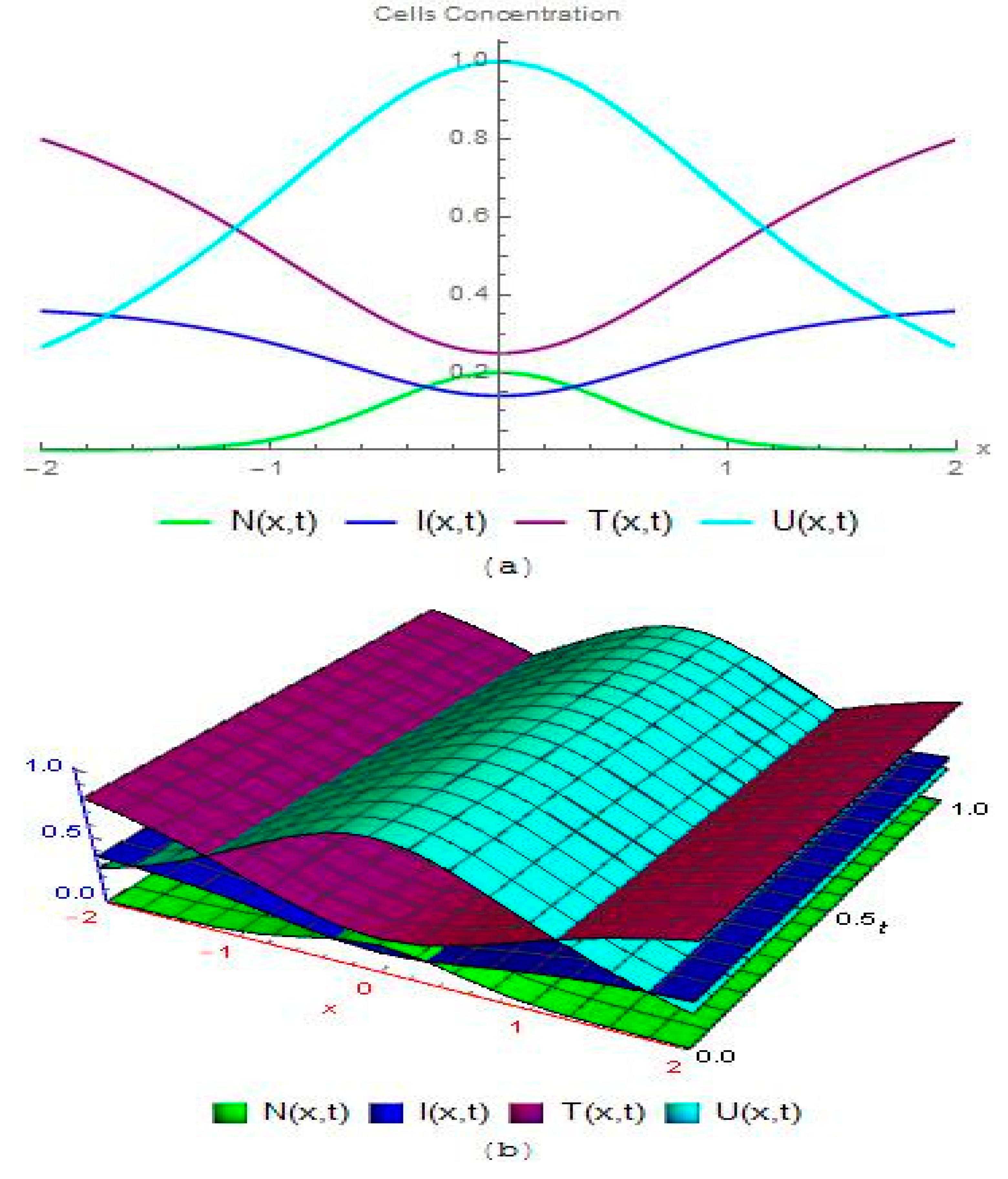
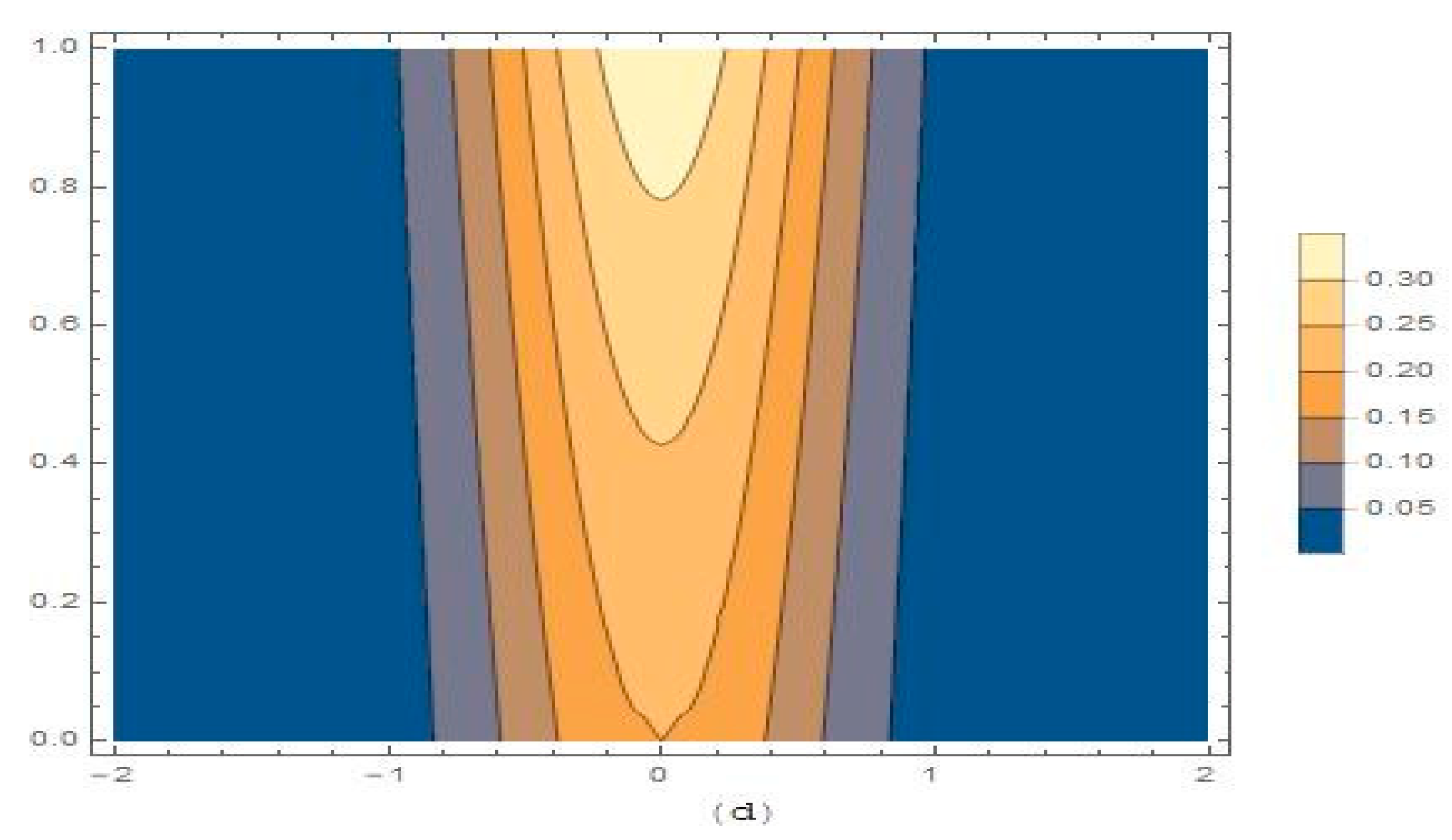
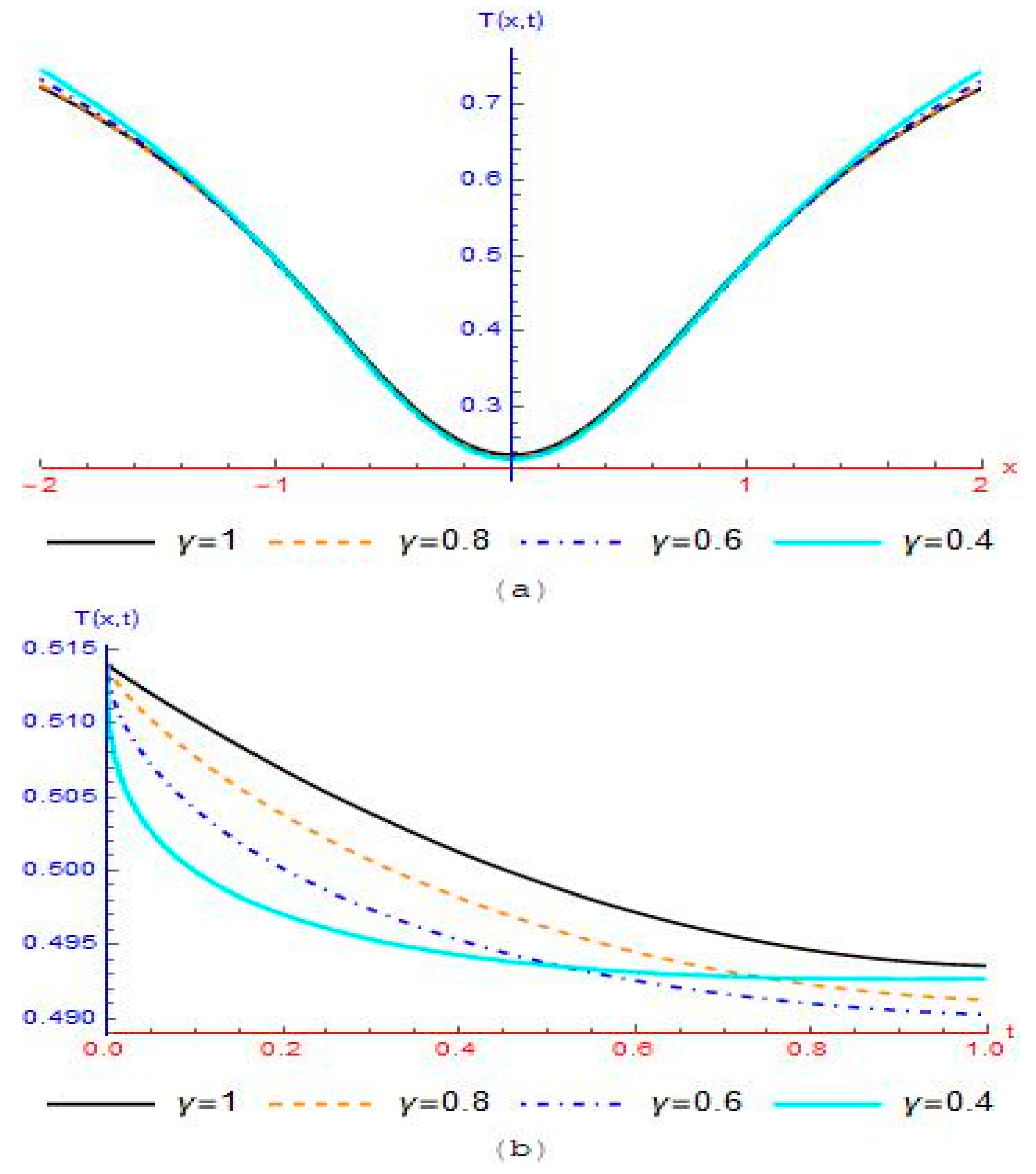
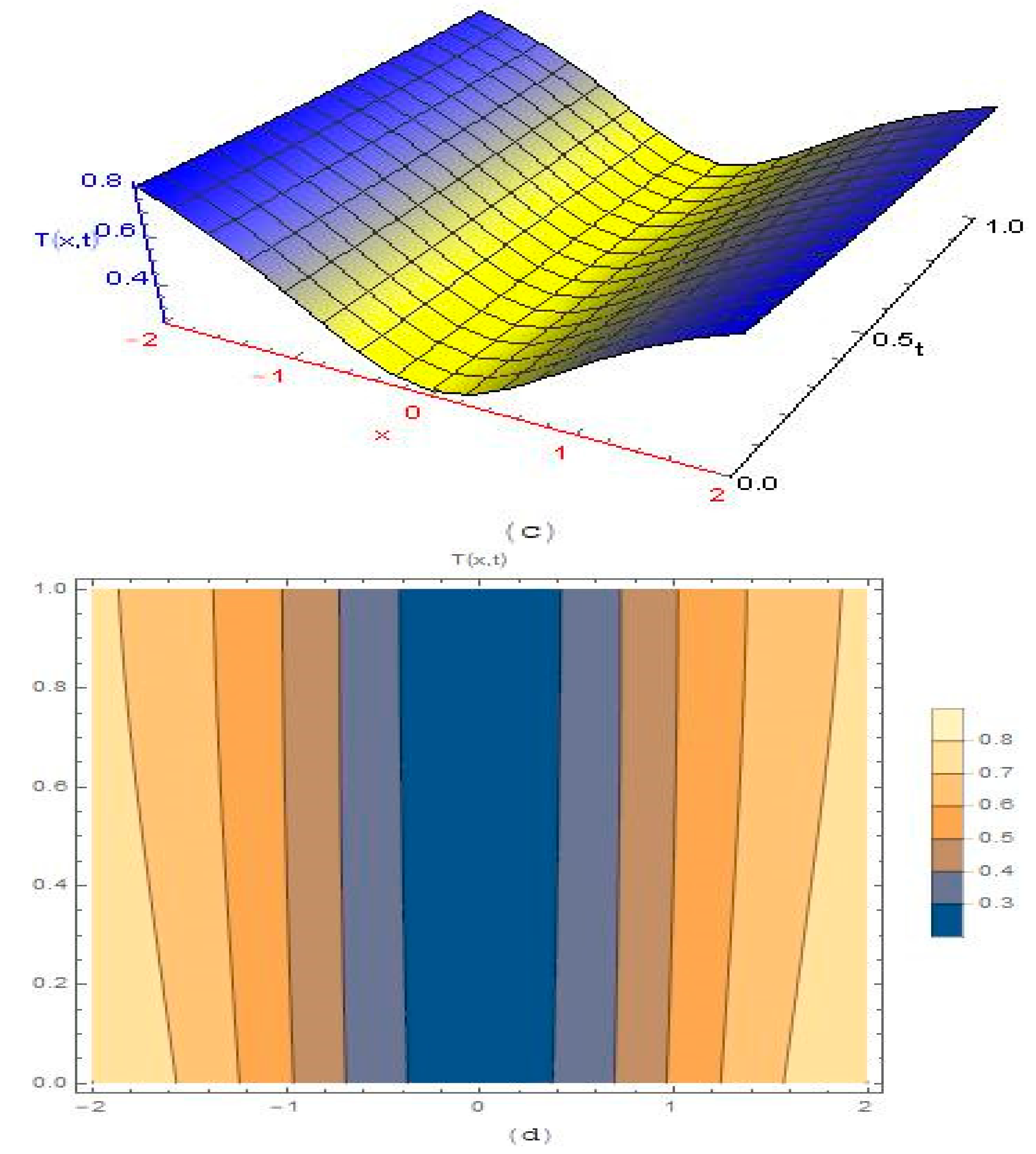
3.2. Modelling Cancer Tumor Based on Cells Concentration

Consider the fractional diffusion equation model of cancer tumor [35].

Case (I): 

The killing percentage of cancer cells K is dependent on the number of cells.

$$\frac{{\partial }^{\gamma }v\left(x, t\right)}{\partial t^{\gamma }}=\frac{{\partial }^{2}v\left(x, t\right)}{\partial x^2}-\frac{2}{x}\frac{\partial v\left(x, t\right)}{\partial x}-v^2\left(x,t\right), x>0, 2\ge \gamma \ge 0,$$

(27)

subject to the initial condition:

$$v\left(x,0\right)=x^q.$$

(28)

According to RDTM, the iteration formulas for Equation (27) can be written as follows:

$${v^{\prime }}_{k+1}\left(x\right)=\frac{\mathsf{\Gamma }\left(k\gamma +1\right)}{\mathsf{\Gamma }\left(k\gamma +\gamma +1\right)}\left[\frac{{\partial }^2{v^{\prime }}_k}{\partial x^2}-\frac{2}{x}\frac{\partial {v^{\prime }}_k}{\partial x}-{\displaystyle \sum }_{m=0}^k{v^{\prime }}_m{v^{\prime }}_{k-m}\right],$$

(29)

In view of the above iterative formula, we obtain the following solutions:

$$\begin{gathered} {v^{\prime }}_0\left(x\right)=x^q, \\ {v^{\prime }}_1\left(x\right)=\frac{\left(-3+q\right)q{x}^{-2+q}-x^{2q}}{\mathsf{\Gamma }\left[1+\gamma \right]}, \\ {v^{\prime }}_2\left(x\right)=\frac{x^{-4+q}\left(-10q^3+q^4+2x^{4+2q}+q^2\left(31-6x^{2+q}\right)+6q\left(-5+2x^{2+q}\right)\right)}{\mathsf{\Gamma }\left[1+2\gamma \right]}, \end{gathered}$$

$$\begin{array}{l}{v^{\prime }}_3\left(x\right)=\frac{1}{\mathsf{\Gamma }\left[1+3\gamma \right]} (-840q{x}^{-6+q}+1198q^2{x}^{-6+q}-651q^3{x}^{-6+q}+169q^4{x}^{-6+q}\\ \hspace{1em}\hspace{1em}\hspace{1em}\hspace{1em}\hspace{1em}-21q^5{x}^{-6+q}+q^6{x}^{-6+q}-4x^{4q}+180q{x}^{-4+2q}-290q^2{x}^{-4+2q}\\ \hspace{1em}\hspace{1em}\hspace{1em}\hspace{1em}\hspace{1em}+152q^3{x}^{-4+2q}-26q^4{x}^{-4+2q}-42q{x}^{-2+3q}+30q^2{x}^{-2+3q}\\ \hspace{1em}\hspace{1em}\hspace{1em}\hspace{1em}\hspace{1em}-\frac{x^{4q}\mathsf{\Gamma }\left[1+2\gamma \right]}{\mathsf{\Gamma }{\left[1+\gamma \right]}^2}-\frac{9q^2{x}^{-4+2q}\mathsf{\Gamma }\left[1+2\gamma \right]}{\mathsf{\Gamma }{\left[1+\gamma \right]}^2}+\frac{6q^3{x}^{-4+2q}\mathsf{\Gamma }\left[1+2\gamma \right]}{\mathsf{\Gamma }{\left[1+\gamma \right]}^2}\\ \hspace{1em}\hspace{1em}\hspace{1em}\hspace{1em}\hspace{1em}-\frac{q^4{x}^{-4+2q}\mathsf{\Gamma }\left[1+2\gamma \right]}{\mathsf{\Gamma }{\left[1+\gamma \right]}^2}-\frac{6q{x}^{-2+3q}\mathsf{\Gamma }\left[1+2\gamma \right]}{\mathsf{\Gamma }{\left[1+\gamma \right]}^2}\\ \hspace{1em}\hspace{1em}\hspace{1em}\hspace{1em}\hspace{1em}+\frac{2q^2{x}^{-2+3q}\mathsf{\Gamma }\mathsf{\Gamma }\left[1+2\gamma \right]}{\mathsf{\Gamma }{\left[1+\gamma \right]}^2})\\ {v^{\prime }}_4\left(x\right)=\frac{x^{-8+q}}{\mathsf{\Gamma }{\left[1+\gamma \right]}^2\mathsf{\Gamma }\left[1+2\gamma \right]\mathsf{\Gamma }\left[1+4\gamma \right]}((-36q^7+q^8+8x^{8+4q}+q^6(538 \\ \hspace{1em}\hspace{1em}\hspace{1em}\hspace{1em}\hspace{1em}-106x^{2+q})+2q^5\left(-2160+611x^{2+q}\right)+q^4(20089\\ \hspace{1em}\hspace{1em}\hspace{1em}\hspace{1em}\hspace{1em}-5570x^{2+q}+322x^{4+2q})-2q^3(26982-6329x^{2+q}\\ \hspace{1em}\hspace{1em}\hspace{1em}\hspace{1em}\hspace{1em}+656x^{4+2q})+12q\left(-3780+560x^{2+q}-65x^{4+2q}+11x^{6+3q}\right)\\ \hspace{1em}\hspace{1em}\hspace{1em}\hspace{1em}\hspace{1em}-2q^2(-38646+7238x^{2+q}-881x^{4+2q}\\ \hspace{1em}\hspace{1em}\hspace{1em}\hspace{1em}\hspace{1em}+62x^{6+3q}))\mathsf{\Gamma }{\left[1+\gamma \right]}^2\mathsf{\Gamma }\left[1+2\gamma \right]+2x^{2+q}(23q^5-2q^6+x^{6+3q}\\ \hspace{1em}\hspace{1em}\hspace{1em}\hspace{1em}\hspace{1em}+q^3\left(183-54x^{2+q}\right)+6q{x}^{2+q}\left(-5+2x^{2+q}\right)+2q^4(-49\\ \hspace{1em}\hspace{1em}\hspace{1em}\hspace{1em}\hspace{1em}+5x^{2+q})-2q^2\left(63-41x^{2+q}+5x^{4+2q}\right))\mathsf{\Gamma }{\left[1+2\gamma \right]}^2\\ \hspace{1em}\hspace{1em}\hspace{1em}\hspace{1em}\hspace{1em}+2x^{2+q}(13q^5-q^6+2x^{6+3q}+q^3\left(123-40x^{2+q}\right)\\ \hspace{1em}\hspace{1em}\hspace{1em}\hspace{1em}\hspace{1em}+6q{x}^{2+q}\left(-5+3x^{2+q}\right)+q^4\left(-61+7x^{2+q}\right)+q^2(-90\\ \hspace{1em}\hspace{1em}\hspace{1em}\hspace{1em}\hspace{1em}+67x^{2+q}-8x^{4+2q}))\mathsf{\Gamma }\left[1+\gamma \left]\mathsf{\Gamma }\right[1+3\gamma \right]),\end{array}$$

(30)

The values for $k>3$ can also be obtained by similar manner. Now, the inverse transform of ${v^{\prime }}_k\left(x\right)$ is

$$v\left(x, \mathfrak{t}\right)={\displaystyle \sum }_{k=0}^{\infty }{v^{\prime }}_k {\mathfrak{t}}^{k\gamma }={v^{\prime }}_0+{v^{\prime }}_1{\mathfrak{t}}^{\gamma }+{v^{\prime }}_2 {\mathfrak{t}}^{2\gamma }+{v^{\prime }}_3{\mathfrak{t}}^{3\gamma }+{v^{\prime }}_4\left(x\right){\mathfrak{t}}^{4\gamma }+\cdots .$$

(31)

By using the values of a few iterations, we obtain the series form solution.

Case (II): 

The killing percentage of cancer cells K is function of time only.

$$\frac{{\partial }^{\gamma }v\left(x, t\right)}{\partial t^{\gamma }}=\frac{{\partial }^{2}v\left(x, t\right)}{\partial x^2}-{\mathrm{t}}^{2}v\left(x,t\right), x>0, 1\ge \gamma \ge 0,$$

(32)

subject to the initial condition:

$$v\left(x, 0\right)=e^{\mu x}.$$

(33)

According to RDTM, the iteration formulas for Equation (32) can be written as follows:

$${v^{\prime }}_{k+1}\left(x\right)=\frac{\mathsf{\Gamma }\left(k\gamma +1\right)}{\mathsf{\Gamma }\left(k\gamma +\gamma +1\right)}\left[\frac{{\partial }^2{v^{\prime }}_k\left(x\right)}{\partial x^2}-{v^{\prime }}_{k-2}\left(x\right)\right],$$

(34)

In view of above iterative formula, we obtain the following solutions:

$$\begin{gathered} {v^{\prime }}_0\left(x\right)=e^{\mu x}, \\ {v^{\prime }}_1\left(x\right)={\mu }^2\frac{1}{\mathsf{\Gamma }\left(\gamma +1\right)}{e}^{\mu x}, \\ {v^{\prime }}_2\left(x\right)={\mu }^4\frac{1}{\mathsf{\Gamma }\left(2\gamma +1\right)}{e}^{\mu x}, \\ {v^{\prime }}_3\left(x\right)=\frac{\left({\mu }^6-\mathsf{\Gamma }\left[1+2\gamma \right]\right)}{\mathsf{\Gamma }\left[1+3\gamma \right]}{e}^{\mu x}, \\ {v^{\prime }}_4\left(x\right)=\frac{{\mu }^2\left(\mathsf{\Gamma }\left[1+\gamma \right]\left({\mu }^6-\mathsf{\Gamma }\left[1+2\gamma \right]\right)-\mathsf{\Gamma }\left[1+3\gamma \right]\right)}{\mathsf{\Gamma }\left[1+\gamma \right]\mathsf{\Gamma }\left[1+4\gamma \right]}{e}^{\mu x}, \end{gathered}$$

(35)

The values for $k>3$ can also be obtained in a similar manner. Now, the inverse transform of ${v^{\prime }}_k\left(x\right)$ is given as:

$$v\left(x, \mathfrak{t}\right)={\displaystyle \sum }_{k=0}^{\infty }{v^{\prime }}_k {\mathfrak{t}}^{k\gamma }={v^{\prime }}_0+{v^{\prime }}_1{\mathfrak{t}}^{\gamma }+{v^{\prime }}_2 {\mathfrak{t}}^{2\gamma }+{v^{\prime }}_3{\mathfrak{t}}^{3\gamma }+{v^{\prime }}_4\left(x\right){\mathfrak{t}}^{4\gamma }+\cdots .$$

(36)

By using the values of a few iterations, we obtain the series form solution.

Case (III): 

The killing percentage of cancer cells K is function of space only.

$$\frac{{\partial }^{\gamma }v\left(x, t\right)}{\partial t^{\gamma }}=\frac{{\partial }^{2}v\left(x, t\right)}{\partial x^2}-\frac{2}{x^2}v\left(x,t\right), x>0, 1\ge \gamma \ge 0,$$

(37)

subject to the initial condition:

$$v\left(x, 0\right)=v\left(x, 0\right)=\frac{a}{x}+b{x}^2.$$

(38)

According to RDTM, the iteration formulas for Equation (37) can be written as follows:

$${v^{\prime }}_{k+1}\left(x\right)=\frac{\mathsf{\Gamma }\left(k\gamma +1\right)}{\mathsf{\Gamma }\left(k\gamma +\gamma +1\right)}\left[\frac{{\partial }^2{v^{\prime }}_k\left(x\right)}{\partial x^2}-\frac{2}{x^2}{v^{\prime }}_k\left(x\right)\right],$$

(39)

In view of the above iterative formula, we obtain the following solutions:

$$\begin{gathered} {v^{\prime }}_0\left(x\right)=\frac{a}{x}+b{x}^2, \\ {v^{\prime }}_i\left(x\right)=0, i=1, 2, 3,\dots \dots \end{gathered}$$

(40)

Now, the inverse transform of ${v^{\prime }}_k\left(x\right)$ is:

$$v\left(x, \mathfrak{t}\right)={\displaystyle \sum }_{k=0}^{\infty }{v^{\prime }}_k {\mathfrak{t}}^{k\gamma }={v^{\prime }}_0+{v^{\prime }}_1{\mathfrak{t}}^{\gamma }+{v^{\prime }}_2 {\mathfrak{t}}^{2\gamma }+{v^{\prime }}_3{\mathfrak{t}}^{3\gamma }+{v^{\prime }}_4\left(x\right){\mathfrak{t}}^{4\gamma }+\cdots .$$

(41)

On putting the values of a few iterations, we obtain the series form solution.

4. Results and Discussion

In order to illustrate the preciseness and effectiveness of the proposed methodology, numerical simulations of two cancer tumor models were carried out. Furthermore, different graphs were drawn to examine the behavior of the obtained solutions.

Two- and three-dimensional comparisons of the initial distribution of normal, tumor, immune, and drug cells are presented in Figure 1. Figure 2a,b represent the behavior of RDTM solution $N\left(x,t\right)$ at $t=0.5$ and $x=1$, respectively, for varied values of $\gamma$, while Figure 2c,d present the three-dimensional contour plots of the RDTM solution $N\left(x,t\right)$, respectively, at $-2\le x\le 2$ and $0\le t\le 1$. Through these plots, we can see that the normal cells are highest at $x=0$ and decrease continuously towards the invasive fronts, i.e., at $x=-2$ and $x=2$. Similarly, Figure 3 shows the behavior of the RDTM solution $T\left(x,t\right)$ tumor cells at $t=0.5$ and $x=1$ for different values of $\gamma$, and we can see that the tumor cells are lowest at $x=0$ but increase continuously towards the invasive fronts, i.e., $x=-2$ and $x=2.$ In Figure 4, the variation of $I\left(x,t\right)$ immune cells with respect to $x$ and $t$ at $\gamma =0.4, 0.6, 0.8$ and $1$ is presented. Figure 5a,b describe the behavior of chemotherapeutic drugs $U\left(x,t\right)$ at $t=0.5$ and $x=1$, respectively, for varied values of non-integer order, while Figure 5c,d explore the concentration of drug cells with respect to $t$ and $x$. These graphics show that the concentration of drug cells is higher at $x=0$ and lower towards the invasive fronts. In Figure 6, two and three-dimensional comparison graphics of RDTM solutions $N\left(x,t\right), T\left(x,t\right), I\left(x,t\right)$ and $U\left(x,t\right)$ are presented. Figure 7a depicts a two-dimensional graphic of tumor cells in the absence of chemotherapeutic drugs at various times, whereas Figure 7b depicts a two-dimensional plot of tumor cells in the presence of drugs at various times, and it is clear from the figures that the concentration of tumor cells is lower in the presence of chemotherapeutic drugs than in the absence of chemotherapeutic drugs. This behavior of tumor cells is explained by the fact that chemotherapeutic drugs enable the body’s defense system to transport more immune cells to the infected area. This represents a step forward in the treatment of cancer tumor by establishing the correlation of chemotherapy drugs while boosting immunity against the specific cancer. The per capita growth rates are represented by $r_i$, where $r_1$ indicates the tumor cell’s parameter while $r_2$ indicates the normal cell’s parameter. In Figure 8, the variation of $T\left(x,t\right)$ tumor cells and $N\left(x,t\right)$ normal cells with respect to per capita growth rates $r_1$ and $r_2$ at $\gamma =1$ is shown. In the above graphs, the values of fractional cell kill $a_1, a_2, a_3$ are considered as 0.2, 0.3, and 0.1, respectively, while the carrying capacity $b_1, b_2$ are considered as 1 and 0.81, respectively. The parameters $c_1, c_2, c_3,c_4$ are taken as 1, 0.55, 0.9, and 1, respectively. $d_1=0.2$ and $d_2=1$ are the deathrate values taken in this work. The values for the immune source rate $\sigma$, the immune threshold rate $\beta$, and the immune response rate $\rho$ are considered as 0.33, 0.3, and 0.2, correspondingly. The values for diffusion coefficients $D_N,D_T,D_I \mathrm{and} D_U$ are 0.001, 0.001, 0.001 and 0.001, respectively.. Finally, it is concluded that the stability of the model is greatly influenced by the aforementioned parameters utilized in the governing equations. The theory of fractional calculus can be effectively used to explain the dynamics of the cancer treatment impact model, which depends on both the time instant and the time history. We discover that a more capable and realistic model can be realized by considering the Caputo-fractional derivatives.

Figure 9a,b shows that the concentration of cancerous cells reduces at $0\le t\le 1$ and $0\le t\le 2$ for varied values of fractional order $\gamma$. In Figure 9c, the concentration of diseased cells starts to increase for some values of $\gamma$, and Figure 9d shows that the concentration of cells still increases for some values of fractional-order gamma at $0\le t\le 10$, but this is not the case for $\gamma =1.75$. At $\gamma =1.75$, the amount of cancer cells decreases for every value of t. So, the best possible fractional-order case for model 4.2 (I) is $\gamma =1.75$. As the time increases, the cancer cells decrease at $\gamma =1.75$, and can be removed from the body after a specific time. Figure 10a,b show the two-dimensional and three-dimensional plots of the RDTM solution $v\left(x,t\right)$ for case (II). In these figures, we check the behavior of disease cells with respect to time by fixing the value of t at varied values of fractional-order gamma. It is seen that the concentration of cells decreases for every value of fractional-order gamma, although $\gamma =1$ yielded the best results. Figure 11a,b explore a reduction in the concentration of cancerous cells, and the influence of fractional order is not noticeable here, but that does not negate its significance. Finally, it is concluded that the killing rate of cancerous cells is dependent on the cell’s concentration.

5. Conclusions

In our work, we successfully implemented the reduced differential transform method (RDTM) for the solution of two fractional cancer tumor models in the Caputo sense. First, the system of four coupled partial differential equation model described the effect of chemotherapeutic drugs in cancer treatment and, second, the cancer model that described the different cases of killing rate $K$ of cancer cells (the killing percentage of cancer cells $K$ (I) is dependent on the number of cells, (II) is a function of time alone, and (III) is a function of space only). It is noted that the method gave series form solutions which converge sharply, and that an increase in the number of terms will increase the solution efficiency. Graphical results show that the obtained solution results agreed with those given in [1,37], and that RDTM is a very straightforward technique does not require any linearization, discretization, perturbation, or restrictive suppositions. In the first model, in the presence of chemotherapeutic drugs, the percentage of tumors cells started to decrease and that of immune cells and normal cells increased. This presents a breakthrough in the treatment of cancer tumor by establishing the correlation of chemotherapy drugs while boosting immunity against the specific cancer. The graphical results of the second model (Case I) show that the concentration of cancerous cells decreases with time at $\gamma =1.75$, and can be removed from the body after a specific phase. It is prospectively important for oncologists to determine at which phase the cancer would be lowered or severe, which is very helpful in the treatment. This means that $\gamma =1.75$ is a suitable fractional order for the selected model. Finally, it is concluded that the selected system parameters influence the stability of the model. The fractional derivative is a useful tool for analyzing the behavior of cancer tumor models, depending on the memory or time history. We discover that a more capable and realistic model can be stabilized by considering the Caputo-fractional derivatives. Because of the power law form of the Caputo’s kernel, namely $h_C\left(t, \beta \right)=\frac{t^{-\beta }}{\mathsf{\Gamma }\left(1-\beta \right)}, 0<\beta <1,$ the memory effects are stronger at small values of time, t. Moreover, it is observed that RDTM is a powerful technique that can be utilized to solve other nonlinear fractional-order differential equations emerging in the field of biological sciences.

References

1. Ansarizadeh, F.; Singh, M.; Richards, D. Modelling of tumor cells regression in response to chemotherapeutic treatment. Appl. Math. Model. 2017, 48, 96–112. [Google Scholar] [CrossRef]
2. Bagley, R.L.; Torvik, P.J. Fractional calculus-a different approach to the analysis of viscoelastically damped structures. AIAA J. 1983, 21, 741–748. [Google Scholar] [CrossRef]
3. Ishteva, M.; Boyadjiev, L.; Scherer, R. On the Caputo operator of fractional calculus and C-Laguerre functions. Math. Sci. Res. J. 2005, 9, 161. [Google Scholar]
4. Kuznetsov, V.A.; Knott, G.D. Modeling tumor regrowth and immunotherapy. Math. Comput. Model. 2001, 33, 1275–1287. [Google Scholar] [CrossRef]
5. De Vladar, H.P.; González, J.A. Dynamic response of cancer under the influence of immunological activity and therapy. J. Theor. Biol. 2004, 227, 335–348. [Google Scholar] [CrossRef]
6. D’Onofrio, A. Metamodeling tumor-immune system interaction, tumor evasion and immunotherapy. Math. Comput. Model. 2008, 47, 614–637. [Google Scholar] [CrossRef]
7. Parish, C.R. Cancer immunotherapy: The past, the present and the future. Immunol. Cell Biol. 2003, 81, 106–113. [Google Scholar] [CrossRef]
8. Attia, N.; Akgül, A.; Seba, D.; Nour, A. Reproducing kernel Hilbert space method for the numerical solutions of fractional cancer tumor models. Math. Methods Appl. Sci. 2020, 1–22. [Google Scholar] [CrossRef]
9. Veeresha, P.; Prakasha, D.G.; Baskonus, H.M. New numerical surfaces to the mathematical model of cancer chemotherapy effect in Caputo fractional derivatives. Chaos Interdiscip. J. Nonlinear Sci. 2019, 29, 013119. [Google Scholar] [CrossRef]
10. Dokuyucu, M.A.; Celik, E.; Bulut, H.; Baskonus, H.M. Cancer treatment model with the Caputo-Fabrizio fractional derivative. Eur. Phys. J. Plus 2018, 133, 92. [Google Scholar] [CrossRef]
11. Arfan, M.; Shah, K.; Ullah, A.; Shutaywi, M.; Kumam, P.; Shah, Z. On Fractional Order Model of Tumor Dynamics with Drug interventions under Nonlocal Fractional Derivative. Results Phys. 2021, 21, 103783. [Google Scholar] [CrossRef]
12. Lee, H.G.; Kim, Y.; Kim, J. Mathematical model and its fast numerical method for the tumor growth. Math. Biosci. Eng. 2015, 12, 1173. [Google Scholar] [CrossRef] [PubMed]
13. Kolev, M.; Zubik-Kowal, B. Numerical solutions for a model of tissue invasion and migration of tumour cells. Comput. Math. Methods Med. 2011, 2011, 452320. [Google Scholar] [CrossRef] [PubMed]
14. Garrido, M.L.K.; Breitenbach, T.; Chudej, K.; Borzì, A. Modeling and numerical solution of a cancer therapy optimal control problem. Appl. Math. 2018, 9, 985–1004. [Google Scholar] [CrossRef]
15. Yasir, M.; Ahmad, S.; Ahmed, F.; Aqeel, M.; Akbar, M.Z. Improved numerical solutions for chaotic-cancer-model. AIP Adv. 2017, 7, 015110. [Google Scholar] [CrossRef]
16. Maddalena, L.; Ragni, S. Existence of solutions and numerical approximation of a non-local tumor growth model. Math. Med. Biol. A J. IMA 2020, 37, 58–82. [Google Scholar] [CrossRef]
17. Sabir, Z.; Munawar, M.; Abdelkawy, M.A.; Raja, M.A.Z.; Ünlü, C.; Jeelani, M.B.; Alnahdi, A.S. Numerical Investigations of the Fractional-Order Mathematical Model Underlying Immune-Chemotherapeutic Treatment for Breast Cancer Using the Neural Networks. Fractal Fract. 2022, 6, 184. [Google Scholar] [CrossRef]
18. Ahmed, N.; Shah, N.A.; Ali, F.; Vieru, D.; Zaman, F.D. Analytical Solutions of the Fractional Mathematical Model for the Concentration of Tumor Cells for Constant Killing Rate. Mathematics 2021, 9, 1156. [Google Scholar] [CrossRef]
19. Bagheri, M.; Khani, A. Analytical Method for Solving the Fractional Order Generalized KdV Equation by a Beta-Fractional Derivative. Adv. Math. Phys. 2020, 2020, 8819183. [Google Scholar] [CrossRef]
20. Fan, K.; Zhou, C. Mechanical Solving a Few Fractional Partial Differential Equations and Discussing the Effects of the Fractional Order. Adv. Math. Phys. 2020, 2020, 3758353. [Google Scholar] [CrossRef]
21. Zhang, H.; Nadeem, M.; Rauf, A.; Hui, Z.G. A novel approach for the analytical solution of nonlinear time-fractional differential equations. Int. J. Numer. Methods Heat Fluid Flow 2020, 31, 1069–1084. [Google Scholar] [CrossRef]
22. Verma, P.; Kumar, M. An Analytical Solution of Linear/Nonlinear Fractional-Order Partial Differential Equations and with New Existence and Uniqueness Conditions. Proc. Natl. Acad. Sci. India Sect. A Phys. Sci. 2020, 92, 47–55. [Google Scholar] [CrossRef]
23. Rehman, M.F.U.; Gu, Y.; Yuan, W. Exact Analytical Solutions of Nonlinear Fractional Liouville Equation by Extended Complex Method. Adv. Math. Phys. 2020, 2020, 8815363. [Google Scholar] [CrossRef]
24. Khan, H.; Shah, R.; Kumam, P.; Baleanu, D.; Arif, M. Laplace decomposition for solving nonlinear system of fractional order partial differential equations. Adv. Differ. Equ. 2020, 2020, 375. [Google Scholar] [CrossRef]
25. Singh, B.K. Fractional reduced differential transform method for numerical computation of a system of linear and nonlinear fractional partial differential equations. Int. J. Open Probl. Comput. Sci. Math. 2016, 9, 20–38. [Google Scholar] [CrossRef]
26. Khalouta, A.; Kadem, A. A new modification of the reduced differential transform method for nonlinear fractional partial differential equations. J. Appl. Math. Comput. Mech. 2020, 19, 45–58. [Google Scholar] [CrossRef]
27. Jafari, H.; Jassim, H.K.; Moshokoa, S.P.; Ariyan, V.M.; Tchier, F. Reduced differential transform method for partial differential equations within local fractional derivative operators. Adv. Mech. Eng. 2016, 8, 160. [Google Scholar] [CrossRef]
28. Kumar, S.; Baleanu, D. A new numerical method for time fractional non-linear sharma-tasso-oliver equation and klein-Gordon equation with exponential kernel law. Front. Phys. 2020, 8, 136. [Google Scholar] [CrossRef]
29. Albadarneh, R.B.; Zerqat, M.; Batiha, I.M. Numerical solutions for linear and non-linear fractional differential equations. Int. J. Pure Appl. Math. 2016, 106, 859–871. [Google Scholar] [CrossRef]
30. Ali, K.K.; Mohamed, E.M.; Mohamed, E.M. A numerical technique for a general form of nonlinear fractional-order differential equations with the linear functional argument. Int. J. Nonlinear Sci. Numer. Simul. 2021, 22, 83–91. [Google Scholar] [CrossRef]
31. Jafari, H.; Gejji, V.D. Solving a system of nonlinear fractional differential equations using Adomian decomposition. J. Comput. Appl. Math. 2006, 196, 644–651. [Google Scholar] [CrossRef]
32. Oyjinda, P.; Pochai, N. Numerical Simulation of an Air Pollution Model on Industrial Areas by Considering the Influence of Multiple Point Sources. Int. J. Differ. Equ. 2019, 2019, 2319831. [Google Scholar] [CrossRef]
33. Bakkyaraj, T. Lie symmetry analysis of system of nonlinear fractional partial differential equations with Caputo fractional derivative. Eur. Phys. J. Plus 2020, 135, 1–17. [Google Scholar]
34. Ibrahim, R.W.; Elobaid, R.M.; Obaiys, S.J. Symmetric conformable fractional derivative of complex variables. Mathematics 2020, 8, 363. [Google Scholar] [CrossRef]
35. Iskenderoglu, G.; Kaya, D. Symmetry analysis of initial and boundary value problems for fractional differential equations in Caputo sense. Chaos Solitons Fractals 2020, 134, 109684. [Google Scholar] [CrossRef]
36. Yang, Q.; Turner, I.; Liu, F. Analytical and numerical solutions for the time and space-symmetric fractional diffusion equation. ANZIAM J. 2008, 50, C800–C814. [Google Scholar] [CrossRef]
37. Iyiola, O.S.; Zaman, F.D. A fractional diffusion equation model for cancer tumor. AIP Adv. 2014, 4, 107121. [Google Scholar] [CrossRef]
38. Burgess, P.K.; Kulesa, P.M.; Murray, J.D.; Alvord, E.C., Jr. The interaction of growth rates and diffusion coefficients in a three-dimensional mathematical model of gliomas. J. Neuropathol. Exp. Neurol. 1997, 56, 704–713. [Google Scholar] [CrossRef]
39. Moyo, S.; Leach, P.G.L. Symmetry methods applied to a mathematical model of a tumour of the brain. Proc. Inst. Math. NAS Ukr. 2004, 50, 204–210. [Google Scholar]
40. Wise, S.M.; Lowengrub, J.S.; Frieboes, H.B.; Cristini, V. Three-dimensional multispecies nonlinear tumor growth—I: Model and numerical method. J. Theor. Biol. 2008, 253, 524–543. [Google Scholar] [CrossRef]
Figure 1. (a): Two-dimensional plot of initial distribution of immune cells, tumor cells, drug cells, and normal cells. (b): Three-dimensional representation of initial distribution of immune cells, tumor cells, drug cells, and normal cells.
Symmetry 14 01694 g001
Figure 2. (a): Effect of γ on normal cells over the coordinates x. (b): Effect of γ on norma cells under time variations. (c): Three dimensional representation of effect of γ on normal cells. (d): Influence of γ on contour profile of normal cells.
Symmetry 14 01694 g002aSymmetry 14 01694 g002b
Figure 3. (a): Effect of γ on tumor cells over the coordinates x. (b): Effect of γ on tumor cells under time variations. (c): Three dimensional representation of effect of γ on tumor cells. (d): Influence of γ on contour profile of tumor cells.
Symmetry 14 01694 g003aSymmetry 14 01694 g003b
Figure 4. (a): Effect of γ on immune cells over the coordinates x. (b): Effect of γ on immune cells under time variations. (c): Three dimensional representation of effect of γ on immune cells. (d): Influence of γ on contour profile of immune cells.
Symmetry 14 01694 g004aSymmetry 14 01694 g004b
Figure 5. (a): Effect of γ on drug cells over the coordinates x. (b): Effect of γ on drug cells under time variations. (c): Three dimensional representation of effect of γ on drug cells. (d): Influence of γ on contour profile of drug cells.
Symmetry 14 01694 g005aSymmetry 14 01694 g005b
Figure 6. (a): Two dimensional concentration representation of Normal, Immune, Tumor and Drug cells using RDTM. (b): Three dimensional concentration representation of Normal, Immune, Tumor and Drug cells using RDTM.
Symmetry 14 01694 g006
Figure 7. (a): Tumor cells in the absence of drugs with time variation (b): Tumor cells in the presence of drugs with varying time.
Symmetry 14 01694 g007
Figure 8. (a): Effect of per capita growth rate on tumor cells with fixed γ . (b): Effect of per capita growth rate on normal cells with fixed γ .
Symmetry 14 01694 g008aSymmetry 14 01694 g008b
Figure 9. (a): Impact of γ on minimum concentration of Cancer tumor cells v ( x , t ) . (b): Impact of γ on average concentration of Cancer tumor cells v ( x , t ) . (c): Impact of γ on high concentration of Cancer tumor cells v ( x , t ) . (d): Impact of γ on highly dense concentration of Cancer tumor cells v ( x , t ) .
Symmetry 14 01694 g009aSymmetry 14 01694 g009b
Figure 10. (a): Two-dimensional RDTM solution of v ( x , t ) at varied values of γ . (b): Three-dimensional comparison of RDTM solution of v ( x ,   t ) at varied values of γ .
Symmetry 14 01694 g010aSymmetry 14 01694 g010b
Figure 11. (a): Two-dimensional RDTM solution of v ( x , t ) at varied values of γ . (b): Three-dimensional comparison of the RDTM solution of v ( x , t ) at varied values of γ .
Symmetry 14 01694 g011