Article

An Efficient Technique to Solve Time-Fractional Kawahara and Modified Kawahara Equations

by
Pavani Koppala
and
Raghavendar Kondooru
*
Department of Mathematics, School of Advanced Sciences, Vellore Institute of Technology, Vellore 632014, India
*
Author to whom correspondence should be addressed.
Symmetry 2022, 14(9), 1777; https://doi.org/10.3390/sym14091777
Submission received: 19 July 2022 / Revised: 16 August 2022 / Accepted: 21 August 2022 / Published: 26 August 2022

Abstract

:
In this article, we analysed the approximate solutions of the time-fractional Kawahara equation and modified Kawahara equation, which describe the propagation of signals in transmission lines and the formation of nonlinear water waves in the long wavelength region. An efficient technique, namely the natural transform decomposition method, is used in the present study. Fractional derivatives are considered in Caputo, Caputo–Fabrizio, and Atangana–Baleanu operative in the Caputo manner. We have presented numerical results graphically to demonstrate the applicability and efficiency of derivatives with fractional order to depict the water waves in long wavelength regions. The symmetry pattern is a fundamental feature of the Kawahara equation and the symmetrical aspect of the solution can be seen from the graphical representations. The obtained outcomes of the proposed method are compared to those of other well-known numerical techniques, such as the homotopy analysis method and residual power series method. Numerical solutions converge to the exact solution of the Kawahara equations, demonstrating the significance of our proposed method.

1. Introduction

In recent years, the study of nonlinear physical processes has benefited tremendously from the exploration of travelling wave solutions for nonlinear equations. Numerous scientific and engineering disciplines, including fluid mechanics, plasma physics, optical fibres, solid state physics and geology, deal with nonlinear wave processes. One of the significant equations in physics and ocean engineering is the Kawahara equation. The purpose of this research is to investigate the analytical scheme and efficiency of using the natural transform decomposition method (NTDM) on finding the symmetric solutions of the time-fractional Kawahara equation (TFKE) and time fractional modified Kawahara equation (TFMKE), which are given below as follows
D τ μ V + V V ζ + V ζ ζ ζ V ζ ζ ζ ζ ζ = 0 , 0 < μ 1 ,
with
V ( ζ , 0 ) = f ( ζ ) ,
D τ μ V + V 2 V ζ + a V ζ ζ ζ + b V ζ ζ ζ ζ ζ = 0 , 0 < μ 1 ,
with
V ( ζ , 0 ) = g ( ζ ) ,
where a > 0 , b < 0 are nonzero arbitrary constants. Dispersive wave equations are important in both mathematics and physics. In the past few decades, the Kawahara equation (KE) and modified Kawahara equation (MKE) have been a popular and active study topic [1,2,3]. Kawahara proposed the KE for characterising solitary-wave propagation in media in 1972 [4]. Kawahara numerically investigated this kind of equation and found that it has monotone and oscillatory solitary wave solutions. The symmetry pattern and set of conservation laws are two further fundamental features of the Kawahara equation. Symmetries and conservation laws of a generalization of the Kawahara equation were examined in [5]. It can be seen in both plasma magneto-acoustic wave theory and shallow water waves with surface tension. Furthermore, the MKE has numerous applications in capillary-gravity water waves, plasma waves, and other fields [6,7,8,9].
Fractional calculus (FC) allows for the differentiation and integration of arbitrary orders and it has grown in popularity in recent decades in fields such as physics, fluid mechanics, electrical networks, groundwater problems, hepatitis B virus model, HIV dynamics model, biological sciences, diffusive transport, and electromagnetic theory [10,11,12,13,14,15,16]. Some of the applications of FC are control theory [17], dissipation [18], relaxation [19], modelling of processes such anomalous diffusion [20,21], and so on. Many scientists and engineers have worked to use fractional differential equations to examine various biological and physical systems. Solving these equations has proven to be a topic of study and interest for scientists from a wide range of disciplines. Numerous efficient approaches for dealing with such models have been established in the modern area of applied research and engineering. Homotopy analysis method (HAM) [22], variational iteration method (VIM) [23,24], monotone iterative technique [25], homotopy perturbation method (HPM) [26], reproducing kernel Hilbert space method [27,28,29], fractional Newton method [30], extended auxiliary equation mapping method, and extended direct algebraic mapping method [31], Laplace transform method for fuzzy partial differential equations [32], modified Adams–Bashforth method [33], ( m + 1 G ) expansion method [34], modified expansion function method and the sine–Gordon expansion method [35], the sine–Gordon expansion technique, and the modified exp ( Ω ( ζ ) ) -expansion function technique [36], Laplace Adomian decomposition method [37], and several others are some of the most popular numerical and analytical approaches for solving linear and nonlinear fractional differential equations.
Several researchers have recently investigated the TFKE and TFMKE using various of methods and techniques, such as the iterative Laplace transform method [17], the HAM [38] and the new iterative method [39], and the residual power series method (RPSM) [40,41].
To the best of the author’s knowledge, this is the first utilisation of NTDM for the study of Kawahara equations with three derivatives, where the Caputo (C) approach is singular and the Caputo–Fabrizio (CF) and Atangna–Baleanu operative in Caputo sense (ABC) approaches have non-singular kernels. The goal of this study is to solve the TFKE and TFMKE using NTDM. The NTDM developed using two powerful approaches, namely natural transform (NT) and Adomian decomposition method. Round-off errors are avoided with the NTDM since it does not require linearization, assumptions, perturbation or discretization. NTDM can transcend the preceding restrictions and limitations of perturbation techniques, allowing us to analyse strongly nonlinear problems. The limitation of the HPM is that it needs solving the functional equation in each iteration, which can be difficult and time-consuming. VIM has an inherent precision in finding the Lagrange multiplier, corrective function, and stationary conditions for fractional order. Unlike the classic Adomian process, the proposed approach does not include the calculation of the fractional derivative or fractional integrals in the recursive formula, which simplifies the estimation of the series terms. Therefore, this method is thought to be a useful tool for fast and easy solving specific classes of coupled nonlinear partial differential equations (PDEs). This method uses a fast convergence series to offer a solution that can be accurate or approximate. As a result, the NTDM is increasingly being used to solve a wide range of linear and nonlinear PDEs [42,43]. NTDM has been used to study a wide range of physical issues, including fractional order problems, such as the fractional system of ordinary differential equations [44], time fractional Klein–Gordon equation [45], time fractional-order coupled Burgers equations [46], and fractional-order Fisher’s equation [47]. Recently, the Kaup–Kupershmidt equation [48] and Kuramoto–Sivashinsky equations [49] have been studied using the natural decomposition method.
The structure of the paper is summarised as follows. The NT of fundamental definitions as well as some additional results useful in the study of fractional differential equations are presented in Section 2. In Section 3, the basic idea for NTDM is to use fractional derivatives such as C, CF, and ABC. In Section 4, the solutions’ uniqueness and convergence are investigated. Solutions of TFKE and TFMKE employing NTDM are included in Section 5. The numerical results and graphs for the TFKE and TFMKE are presented in Section 6. Lastly, in Section 7, we discuss our conclusions.

2. Basic Definitions

The fractional derivative definitions of C, CF, ABC, and some properties of NT are presented as follows.
Definition 1
([50]). In the Caputo manner, the fractional derivative of f C 1 q is shown as
D τ μ f ( τ ) = d q f ( τ ) d τ q , μ = q N , 1 Γ ( q μ ) 0 τ ( τ ξ ) q μ 1 f q ( ξ ) d ξ , q 1 < μ < q , q N .
Definition 2
([51]). Let 0 < μ < 1 . Fractional CF derivative of order μ is denoted as
C F D τ μ f ( τ ) = 1 1 μ 0 τ f ( ζ ) exp μ ( τ ζ ) 1 μ d ζ , τ 0 .
Definition 3
([52]). Fractional ABC derivative definition of f is as follows
A B C D τ μ f ( τ ) = B [ μ ] 1 μ 0 τ f ( ζ ) E μ μ ( τ ζ ) μ 1 μ d ζ ,
where 0 < μ < 1 . The B [ μ ] is a normalization function and the Mittag-Leffler function is E μ = i = 0 Z i Γ ( μ i + 1 ) .
Definition 4
([53,54]). The NT of the function f ( τ ) is defined as
N + [ f ( τ ) ] = R ( s , u ) = 1 u 0 + e ( s τ u ) f ( τ ) d τ , u , s > 0 .
Definition 5
([55]). NT of D τ μ V ( τ ) by means of C derivative is given as
N + [ 0 C D τ μ V ( τ ) ] = ( s v ) μ N + [ V ( τ ) ] 1 s V ( 0 ) .
Definition 6
([56]). NT of D τ μ V ( τ ) by means of CF derivative is defined as
N + [ 0 C F D τ μ V ( τ ) ] = 1 1 μ + μ ( v s ) N + [ V ( τ ) ] 1 s V ( 0 ) .
Definition 7
([57]). NT of D τ μ V ( τ ) by means of ABC derivative is represented as
N + [ 0 A B C D τ μ V ( τ ) ] = M [ μ ] 1 μ + μ ( v s ) μ N + [ V ( τ ) ] 1 s V ( 0 ) ,
where M [ μ ] is the normalization function such that M [ 0 ] = M [ 1 ] = 1 .

3. Basic Idea of NTDM

We consider the general inhomogeneous nonlinear equation as follows in this section, which contains the basic idea of NTDM.
D τ μ V ( ζ , τ ) = R [ V ( ζ , τ ) ] + F [ V ( ζ , τ ) ] + p ( ζ , τ ) ,
with the initial condition,
V ( ζ , 0 ) = f ( ζ ) .
Here, R is linear, F is nonlinear and p ( ζ , τ ) is the source term. Now, we can use the NT of Equation (12) by taking fractional derivatives of C, CF, and ABC definitions.
NTDM C : By taking the NT of Equation (12) using C derivative, we get
s v μ N + [ V ( ζ , τ ) ] f ( ζ ) s = N + R [ V ( ζ , τ ) ] + F [ V ( ζ , τ ) ] + p ( ζ , τ ) .
By taking inverse NT on Equation (14), we get
V ( ζ , τ ) = N 1 f ( ζ ) s + v s μ N + [ R [ V ( ζ , τ ) ] + F [ V ( ζ , τ ) ] + p ( ζ , τ ) ] .
The nonlinear term can also be expressed as
F [ V ( ζ , τ ) ] = k = 0 A k ,
where A k are the Adomian polynomials of V 0 , V 1 , V 2 , , and can be calculated with the given formula
A k = 1 k ! d k d μ k F k = 0 μ k V k μ = 0 , k = 0 , 1 , 2 , .
Let the infinite series solution V ( ζ , τ ) be of the form
V ( ζ , τ ) = k = 0 V k ( ζ , τ ) .
Now, we substitute Equations (16) and (18) into (15) to obtain
k = 0 V k ( ζ , τ ) = N 1 f ( ζ ) s + N 1 v s μ N + [ p ( ζ , τ ) ] + N 1 v s μ N + R k = 0 V k ( ζ , τ ) + k = 0 A k .
By comparing the two sides of the Equation (19), we get
C V 0 ( ζ , τ ) = N 1 f ( ζ ) s + N 1 v s μ N + [ p ( ζ , τ ) ] , C V 1 ( ζ , τ ) = N 1 v s μ N + [ R [ V 0 ( ζ , τ ) ] + A 0 ] , C V 2 ( ζ , τ ) = N 1 v s μ N + [ R [ V 1 ( ζ , τ ) ] + A 1 ] , C V 3 ( ζ , τ ) = N 1 v s μ N + [ R [ V 2 ( ζ , τ ) ] + A 2 ] , C V k + 1 ( ζ , τ ) = N 1 v s μ N + [ R [ V k ( ζ , τ ) ] + A k ] , k 0 .
By substituting (20) into (18), we get the NTDM C by the series solutions of (12) and (13) as
C V ( ζ , τ ) = C V 0 ( ζ , τ ) + C V 1 ( ζ , τ ) + C V 2 ( ζ , τ ) + .
NTDM C F : By taking NT of Equation (12) using CF derivative, we get
1 1 μ + μ ( v s ) N + [ V ( ζ , τ ) ] f ( ζ ) s = N + [ R [ V ( ζ , τ ) ] + F [ V ( ζ , τ ) ] + p ( ζ , τ ) ] .
By taking inverse NT on Equation (22), we get
V ( ζ , τ ) = N 1 f ( ζ ) s + 1 μ + μ v s N + [ R [ V ( ζ , τ ) ] + F [ V ( ζ , τ ) ] + p ( ζ , τ ) ] .
Now, we substitute Equations (16) and (18) into (23) to obtain
k = 0 V k ( ζ , τ ) = N 1 f ( ζ ) s + N 1 1 μ + μ v s N + [ p ( ζ , τ ) ] + N 1 1 μ + μ v s N + R k = 0 V k ( ζ , τ ) + k = 0 A k .
By comparing the two sides of the Equation (24), we get
C F V 0 ( ζ , τ ) = N 1 f ( ζ ) s + N 1 1 μ + μ v s N + [ p ( ζ , τ ) ] , C F V 1 ( ζ , τ ) = N 1 1 μ + μ v s N + [ R [ V 0 ( ζ , τ ) ] + A 0 ] , C F V 2 ( ζ , τ ) = N 1 1 μ + μ v s N + [ R [ V 1 ( ζ , τ ) ] + A 1 ] , C F V 3 ( ζ , τ ) = N 1 1 μ + μ v s N + [ R [ V 2 ( ζ , τ ) ] + A 2 ] , C F V k + 1 ( ζ , τ ) = N 1 1 μ + μ v s N + [ R [ V k ( ζ , τ ) ] + A k ] , k 0 .
By substituting (25) into (18), we get the NTDM C F by the series solutions of (12) and (13) as
C F V ( ζ , τ ) = C F V 0 ( ζ , τ ) + C F V 1 ( ζ , τ ) + C F V 2 ( ζ , τ ) + .
NTDM A B C : By taking NT of Equation (12) using ABC derivative, we get
M [ μ ] 1 μ + μ v s μ N + [ V ( ζ , τ ) ] f ( ζ ) s = N + [ R [ V ( ζ , τ ) ] + F [ V ( ζ , τ ) ] + p ( ζ , τ ) ] .
By taking inverse NT on Equation (27), we get
V ( ζ , τ ) = N 1 f ( ζ ) s + 1 μ + μ v s μ M [ μ ] N + [ R [ V ( ζ , τ ) ] + F [ V ( ζ , τ ) ] + p ( ζ , τ ) ] .
Now, we substitute Equations (16) and (18) into (28) to obtain
k = 0 V k ( ζ , τ ) = N 1 f ( ζ ) s + N 1 1 μ + μ v s μ M [ μ ] N + [ p ( ζ , τ ) ] + N 1 1 μ + μ v s μ M [ μ ] N + R k = 0 V k ( ζ , τ ) + k = 0 A k .
By comparing the two sides of the Equation (29), we get
A B C V 0 ( ζ , τ ) = N 1 f ( ζ ) s + N 1 1 μ + μ v s μ M [ μ ] N + [ p ( ζ , τ ) ] , A B C V 1 ( ζ , τ ) = N 1 1 μ + μ v s μ M [ μ ] N + [ R [ V 0 ( ζ , τ ) ] + A 0 ] , A B C V 2 ( ζ , τ ) = N 1 1 μ + μ v s μ M [ μ ] N + [ R [ V 1 ( ζ , τ ) ] + A 1 ] , A B C V 3 ( ζ , τ ) = N 1 1 μ + μ v s μ M [ μ ] N + [ R [ V 2 ( ζ , τ ) ] + A 2 ] , A B C V k + 1 ( ζ , τ ) = N 1 1 μ + μ v s μ M [ μ ] N + [ R [ V k ( ζ , τ ) ] + A k ] , k 0 .
By substituting (30) into (18), we get the NTDM A B C by the series solutions of (12) and (13) as
A B C V ( ζ , τ ) = A B C V 0 ( ζ , τ ) + A B C V 1 ( ζ , τ ) + A B C V 2 ( ζ , τ ) + .

4. Convergence Analysis

In this section, we illustrate convergence and uniqueness of the NTDM C , NTDM C F , and NTDM A B C .
Theorem 1
([57]). The NTDM C solution of (12) is unique when 0 < ( δ 1 + δ 2 ) τ μ Γ ( 1 + μ ) < 1 .
Proof. 
Assume that H = ( C [ I ] , . ) stands ∀ continuous mapping on the Banach space with the norm, specified on I = [ 0 , T ] . For this, we propose the mapping L : H H , we have
V k + 1 C ( ζ , τ ) = V 0 C + N 1 v s μ N + [ R ( V k ( ζ , τ ) ) ] + N 1 v s μ N + [ F ( V k ( ζ , τ ) ) ] , k 0 .
Let us suppose R ( V ) R ( V * ) < δ 1 V V * and F ( V ) F ( V * ) < δ 2 V V * , where δ 1 and δ 2 are Lipschitz constants, respectively, and V and V * are two arbitrary values of the mapping.
L ( V ) L ( V * ) = max τ I | N 1 v s μ N + [ R ( V ) + F ( V ) ] N 1 v s μ N + [ R ( V * ) + F ( V * ) ] | max τ I | N 1 v s μ N + [ R ( V ) R ( V * ) ] + v s μ N + [ F ( V ) F ( V * ) ] | max τ I δ 1 N 1 v s μ N + | V V * | + δ 2 N 1 v s μ N + | V V * | max τ I ( δ 1 + δ 2 ) N 1 v s μ N + | V V * | ( δ 1 + δ 2 ) N 1 v s μ N + V V * = ( δ 1 + δ 2 ) τ μ Γ ( μ + 1 ) V V * .
The mapping is a contraction under the premise 0 < ( δ 1 + δ 2 ) τ μ Γ ( 1 + μ ) < 1 . As a result of the Banach contraction fixed point theorem, there is a unique solution to (12). □
Theorem 2
([57]). When 0 < ( δ 1 + δ 2 ) ( 1 μ + μ τ ) < 1 , then NTDM C F solution to (12) is unique.
Proof. 
This proof has been omitted since it is identical to Theorem 1. □
Theorem 3
([57]). When 0 < ( δ 1 + δ 2 ) ( 1 μ + μ τ μ Γ ( μ + 1 ) ) < 1 , the NTDM A B C solution to (12) is unique.
Proof. 
Because it is similar to Theorem 1, it has been omitted. □
Theorem 4
([57]). The general form of NTDM C solution to (12) will be convergent.
Proof. 
Assume that V m is the mth parital sum and that V m = k = 0 m V k ( ζ , τ ) . First, we demonstrate the V m in Banach space in H is a Cauchy sequence. We obtain this by considering a new form Adomian polynomials.
Now,
V m V q = max τ I | V m V q | = max τ I | r = q + 1 m V r | , q = 1 , 2 , 3 , . max τ I | N 1 v s μ N + r = q + 1 m ( R ( V r 1 ) + F ( V r 1 ) ) | = max τ I | N 1 v s μ N + r = q m 1 R ( V r ) + F ( V r ) | max τ I | N 1 v s μ N + [ R ( V m 1 ) R ( V q 1 ) ] | + max τ I | N 1 v s μ N + [ F ( V m 1 ) F ( V q 1 ) ] | δ 1 max τ I | N 1 v s μ [ N + [ R ( V m 1 ) R ( V q 1 ) ] ] | + δ 2 max τ I | N 1 v s μ [ N + [ F ( V m 1 ) F ( V q 1 ) ] ] | = ( δ 1 + δ 2 ) τ μ Γ ( μ + 1 ) V m 1 V q 1 .
Consider m = q + 1 , then
V q + 1 V q δ V q V q 1 δ 2 V q 1 V q 2 δ q V 1 V 0 ,
where δ = ( δ 1 + δ 2 ) τ μ Γ ( μ + 1 ) . Analogously, we get the triangular inequality.
V m V q V q + 1 V q + V q + 2 V q + 1 + + V m V m 1 ( δ q + δ q + 1 + + δ m 1 ) V 1 V 0 δ q 1 δ m q 1 δ V 1 .
As 0 < δ < 1 , we get 1 δ m q < 1 . Therefore,
V m V q δ q 1 δ max τ I V 1 .
However, V 1 < . Thus, as q , then V m V q 0 . Hence, V m is a Cauchy sequence in H. As a result, the series V m is convergent. □
Theorem 5
([57]). The (12) NTDM C F solution is convergent.
Proof. 
The proof has been omitted since it is similar to Theorem 4. □
Theorem 6
([57]). The (12) NTDM A B C solution is convergent.
Proof. 
The proof has been omitted since it is similar to Theorem 4. □

5. Solutions for TFKE and TFMKE

In this section, we obtain the following solutions of TFKE and TFMKE using NTDM by taking C, CF, and ABC derivatives.
Example 1.
Consider the TFKE as of the form
D τ μ V + V V ζ + V ζ ζ ζ V ζ ζ ζ ζ ζ = 0 ,
with initial condition,
V ( ζ , 0 ) = 105 169 sech 4 ζ 2 13 .
If μ = 1 , then the exact solution is [38],
V ( ζ , τ ) = 105 169 sech 4 1 2 13 ζ 36 τ 169 .
NTDM C : We obtain the following solutions of NTDM C derivative as
C V 0 ( ζ , τ ) = 105 169 sech 4 ζ 2 13 , C V 1 ( ζ , τ ) = 7560 13 τ μ sinh 13 ζ 26 371,293 Γ 1 + μ cosh 5 13 ζ 26 , C V 2 ( ζ , τ ) = 136,080 τ 2 μ 2 sinh 13 ζ 26 1 ( 2 sinh 13 ζ 26 + 1 62,748,517 Γ 1 + 2 μ sinh 2 13 ζ 26 + 1 3 ,
by substituting C V 0 ( ζ , τ ) , C V 1 ( ζ , τ ) , C V 2 ( ζ , τ ) , values in (21), we obtain the approximate solution as
C V ( ζ , τ ) = 105 169 sech 4 ζ 2 13 + 7560 13 τ μ sinh 13 ζ 26 371,293 Γ 1 + μ cosh 5 13 ζ 26 + 136,080 τ 2 μ 2 sinh 13 ζ 26 1 ( 2 sinh 13 ζ 26 + 1 62,748,517 Γ 1 + 2 μ sinh 2 13 ζ 26 + 1 3 + .
NTDM C F : We obtain the following solutions of NTDM C F derivative as
C F V 0 ( ζ , τ ) = 105 169 sech 4 ζ 2 13 , C F V 1 ( ζ , τ ) = 7560 13 sinh 13 ζ 26 1 μ + μ τ 371,293 cosh 5 13 ζ 26 , C F V 2 ( ζ , τ ) = 2 cosh 13 ζ 13 3 62,748,517 sinh 2 13 ζ 26 + 1 3 ( 136,080 272,160 μ + 136,080 μ 2 + 272,160 μ τ 272,160 μ 2 τ + 68,040 μ 2 τ 2 ) ,
by substituting C F V 0 ( ζ , τ ) , C F V 1 ( ζ , τ ) , C F V 2 ( ζ , τ ) , values in (26), we obtain the approximate solution as
C F V ( ζ , τ ) = 105 169 sech 4 ζ 2 13 + 7560 13 sinh 13 ζ 26 1 μ + μ τ 371,293 cosh 5 13 ζ 26 + 2 cosh 13 ζ 13 3 62,748,517 sinh 2 13 ζ 26 + 1 3 ( 136,080 272,160 μ + 136,080 μ 2 + 272,160 μ τ 272,160 μ 2 τ + 68,040 μ 2 τ 2 ) + .
NTDM A B C : We obtain the following solutions of NTDM A B C derivative as
A B C V 0 ( ζ , τ ) = 105 169 sech 4 ζ 2 13 , A B C V 1 ( ζ , τ ) = 7560 13 sinh 13 ζ 26 Γ 1 + μ μ Γ 1 + μ + μ τ μ 371,293 Γ 1 + μ cosh 13 ζ 26 5 , A B C V 2 ( ζ , τ ) = 136,080 2 sinh 13 ζ 26 1 2 sinh 13 ζ 26 + 1 62,080,517 Γ 1 + μ Γ ( 1 + 2 μ ) sinh 2 13 ζ 26 + 1 3 ( Γ 1 + μ Γ ( 1 + 2 μ ) 2 μ Γ 1 + μ Γ ( 1 + 2 μ ) + 2 μ τ μ Γ ( 1 + 2 μ ) + μ 2 Γ 1 + μ Γ ( 1 + 2 μ ) 2 μ 2 τ μ Γ ( 1 + 2 μ ) + μ 2 τ 2 μ Γ 1 + μ ) ,
by substituting A B C V 0 ( ζ , τ ) , A B C V 1 ( ζ , τ ) , A B C V 2 ( ζ , τ ) , values in (31), we obtain the approximate solution as
A B C V ( ζ , τ ) = 105 169 sech 4 ζ 2 13 + 7560 13 sinh 13 ζ 26 Γ 1 + μ μ Γ 1 + μ + μ τ μ 371,293 Γ 1 + μ cosh 13 ζ 26 5 + 136,080 2 sinh 13 ζ 26 1 2 sinh 13 ζ 26 + 1 62,748,517 Γ 1 + μ Γ ( 1 + 2 μ ) sinh 2 13 ζ 26 + 1 3 ( Γ 1 + μ Γ ( 1 + 2 μ ) 2 μ Γ 1 + μ Γ ( 1 + 2 μ ) + 2 μ τ μ Γ ( 1 + 2 μ ) + μ 2 Γ 1 + μ Γ ( 1 + 2 μ ) 2 μ 2 τ μ Γ ( 1 + 2 μ ) + μ 2 τ 2 μ Γ 1 + μ ) + .
Example 2.
Consider the TFMKE as of the form
D τ μ V + V 2 V ζ + a V ζ ζ ζ + b V ζ ζ ζ ζ ζ = 0 ,
with initial condition,
V ( ζ , 0 ) = 3 a 10 b sech 2 ( P ζ ) .
If μ = 1 , then the exact solution is [38],
V ( ζ , τ ) = 3 a 10 b sech 2 ( P ( ζ l τ ) ) , P = 1 2 a 5 b , l = 25 b 4 a 2 25 b .
NTDM C : We obtain the following solutions of NTDM C derivative as
C V 0 ( ζ , τ ) = 3 a 10 b sech 2 1 2 a 5 b ζ , C V 1 ( ζ , τ ) = 6 2 a 3 τ μ sinh 5 ζ a b 10 a b 125 b 3 / 2 Γ 1 + μ cos 5 a ζ 10 b 3 , C V 2 ( ζ , τ ) = 6 10 a 11 / 2 τ 2 μ 15,625 ( b ) 7 2 cos 8 5 a ζ 10 b Γ ( 1 + 2 μ ) ( 45 a sinh 2 5 ζ a b 10 2 a + 51 a sin 2 5 a ζ 10 b 51 a sin 4 5 a ζ 10 b + 2 a sin 6 5 a ζ 10 b + 6 b sin 5 a ζ 10 b sinh 5 ζ a b 10 a b 57 b sin 3 5 a ζ 10 b × sinh 5 ζ a b 10 a b + 6 b sin 5 5 a ζ 10 b sinh 5 ζ a b 10 a b ) ,
by substituting C V 0 ( ζ , τ ) , C V 1 ( ζ , τ ) , C V 2 ( ζ , τ ) , values in (21), we obtain the approximate solution as
C V ( ζ , τ ) = 3 a 10 b sech 2 1 2 a 5 b ζ + 6 2 a 3 τ μ sinh 5 ζ a b 10 a b 125 b 3 / 2 Γ 1 + μ cos 5 a ζ 10 b 3 + 6 10 a 11 / 2 τ 2 μ 15,625 ( b ) 7 2 cos 8 5 a ζ 10 b Γ ( 1 + 2 μ ) ( 45 a sinh 2 5 ζ a b 10 2 a + 51 a sin 2 5 a ζ 10 b 51 a sin 4 5 a ζ 10 b + 2 a sin 6 5 a ζ 10 b + 6 b sin 5 a ζ 10 b sinh 5 ζ a b 10 a b 57 b sin 3 5 a ζ 10 b × sinh 5 ζ a b 10 a b + 6 b sin 5 5 a ζ 10 b sinh 5 ζ a b 10 a b ) + .
NTDM C F : We obtain the following solutions of NTDM C F derivative as
C F V 0 ( ζ , τ ) = 3 a 10 b sech 2 1 2 a 5 b ζ , C F V 1 ( ζ , τ ) = 6 2 a 3 sinh 5 ζ a b 10 a b 1 μ + μ τ 125 b 3 / 2 cos 5 a ζ 10 b 3 , C F V 2 ( ζ , τ ) = 3 10 a 11 / 2 2 4 μ + 2 μ 2 + 4 μ τ 4 μ 2 τ + μ 2 τ 2 15,625 b 7 / 2 cos 8 5 a ζ 10 b ( 45 a sinh 2 5 ζ a b 10 2 a + 51 a sin 2 5 a ζ 10 b 51 a sin 4 5 a ζ 10 b + 2 a sin 6 5 a ζ 10 b + 6 b sin 5 a ζ 10 b × sinh 5 ζ a b 10 a b 57 b sin 3 5 a ζ 10 b sinh 5 ζ a b 10 a b + 6 b sin 5 5 a ζ 10 b sinh 5 ζ a b 10 a b ) ,
by substituting C F V 0 ( ζ , τ ) , C F V 1 ( ζ , τ ) , C F V 2 ( ζ , τ ) , values in (26), we obtain the approximate solution as
C F V ( ζ , τ ) = 3 a 10 b sech 2 1 2 a 5 b ζ + 6 2 a 3 sinh 5 ζ a b 10 a b 1 μ + μ τ 125 b 3 / 2 cos 5 a ζ 10 b 3 + 3 10 a 11 / 2 2 4 μ + 2 μ 2 + 4 μ τ 4 μ 2 τ + μ 2 τ 2 15,625 b 7 / 2 cos 8 5 a ζ 10 b ( 45 a sinh 2 5 ζ a b 10 2 a + 51 a sin 2 5 a ζ 10 b 51 a sin 4 5 a ζ 10 b + 2 a sin 6 5 a ζ 10 b + 6 b sin 5 a ζ 10 b × sinh 5 ζ a b 10 a b 57 b sin 3 5 a ζ 10 b sinh 5 ζ a b 10 a b + 6 b sin 5 5 a ζ 10 b sinh 5 ζ a b 10 a b ) + .
NTDM A B C : We obtain the following solutions of NTDM A B C derivative as
A B C V 0 ( ζ , τ ) = 3 a 10 b sech 2 1 2 a 5 b ζ , A B C V 1 ( ζ , τ ) = 6 2 a 3 sinh 5 ζ a b 10 a b Γ 1 + μ μ Γ 1 + μ + μ τ μ 125 b 3 / 2 Γ 1 + μ cos 5 a ζ 10 b 3 , A B C V 2 ( ζ , τ ) = 1 15,625 b 7 / 2 Γ 1 + μ cos 8 5 a ζ 10 b Γ ( 1 + 2 μ ) ( 6 10 a 11 / 2 ( Γ 1 + μ Γ ( 1 + 2 μ ) 2 μ Γ 1 + μ Γ ( 1 + 2 μ ) + 2 μ τ μ Γ ( 1 + 2 μ ) + μ 2 Γ 1 + μ Γ ( 1 + 2 μ ) 2 μ 2 τ μ Γ ( 1 + 2 μ ) + μ 2 τ 2 μ Γ 1 + μ ) × ( 45 a sinh 5 ζ a b 10 2 2 a + 51 a sin 2 5 a ζ 10 b 51 a sin 4 5 a ζ 10 b + 2 a sin 6 5 a ζ 10 b + sinh 5 ζ a b 10 a b × 6 b sin 5 a ζ 10 b 57 b sin 3 5 a ζ 10 b + 6 b sin 5 5 a ζ 10 b ) ) ,
by substituting A B C V 0 ( ζ , τ ) , A B C V 1 ( ζ , τ ) , A B C V 2 ( ζ , τ ) , values in (31), we obtain the approximate solution as
A B C V ( ζ , τ ) = 3 a 10 b sech 2 1 2 a 5 b ζ + 6 2 a 3 sinh 5 ζ a b 10 a b Γ 1 + μ μ Γ 1 + μ + μ τ μ 125 b 3 / 2 Γ 1 + μ cos 5 a ζ 10 b 3 + 1 15,625 b 7 / 2 Γ 1 + μ cos 8 5 a ζ 10 b Γ ( 1 + 2 μ ) ( 6 10 a 11 / 2 ( Γ 1 + μ Γ ( 1 + 2 μ ) 2 μ Γ 1 + μ Γ ( 1 + 2 μ ) + 2 μ τ μ Γ ( 1 + 2 μ ) + μ 2 Γ 1 + μ Γ ( 1 + 2 μ ) 2 μ 2 τ μ Γ ( 1 + 2 μ ) + μ 2 τ 2 μ Γ 1 + μ ) × ( 45 a sinh 5 ζ a b 10 2 2 a + 51 a sin 2 5 a ζ 10 b 51 a sin 4 5 a ζ 10 b + 2 a sin 6 5 a ζ 10 b + sinh 5 ζ a b 10 a b × 6 b sin 5 a ζ 10 b 57 b sin 3 5 a ζ 10 b + 6 b sin 5 5 a ζ 10 b ) ) + .

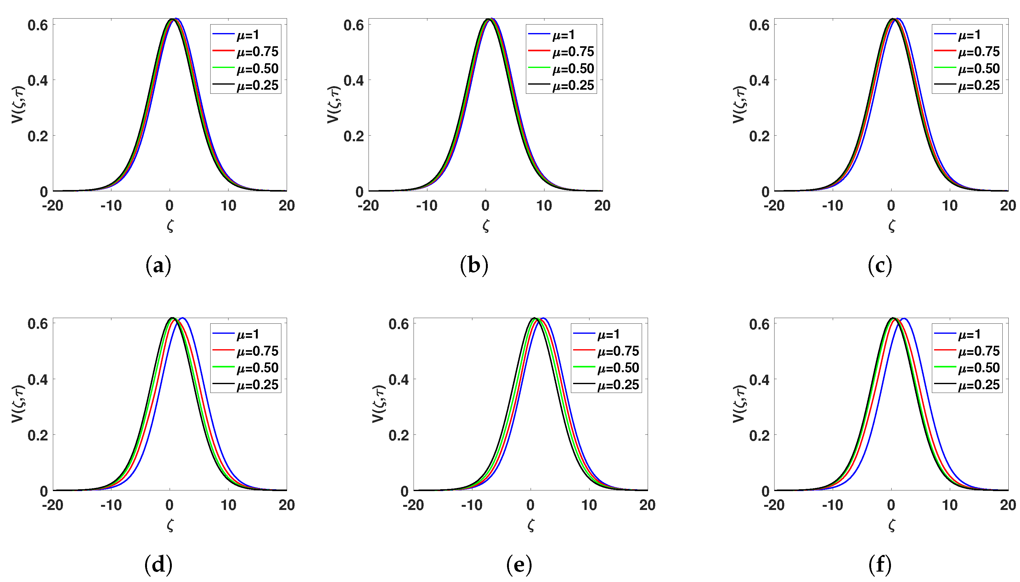
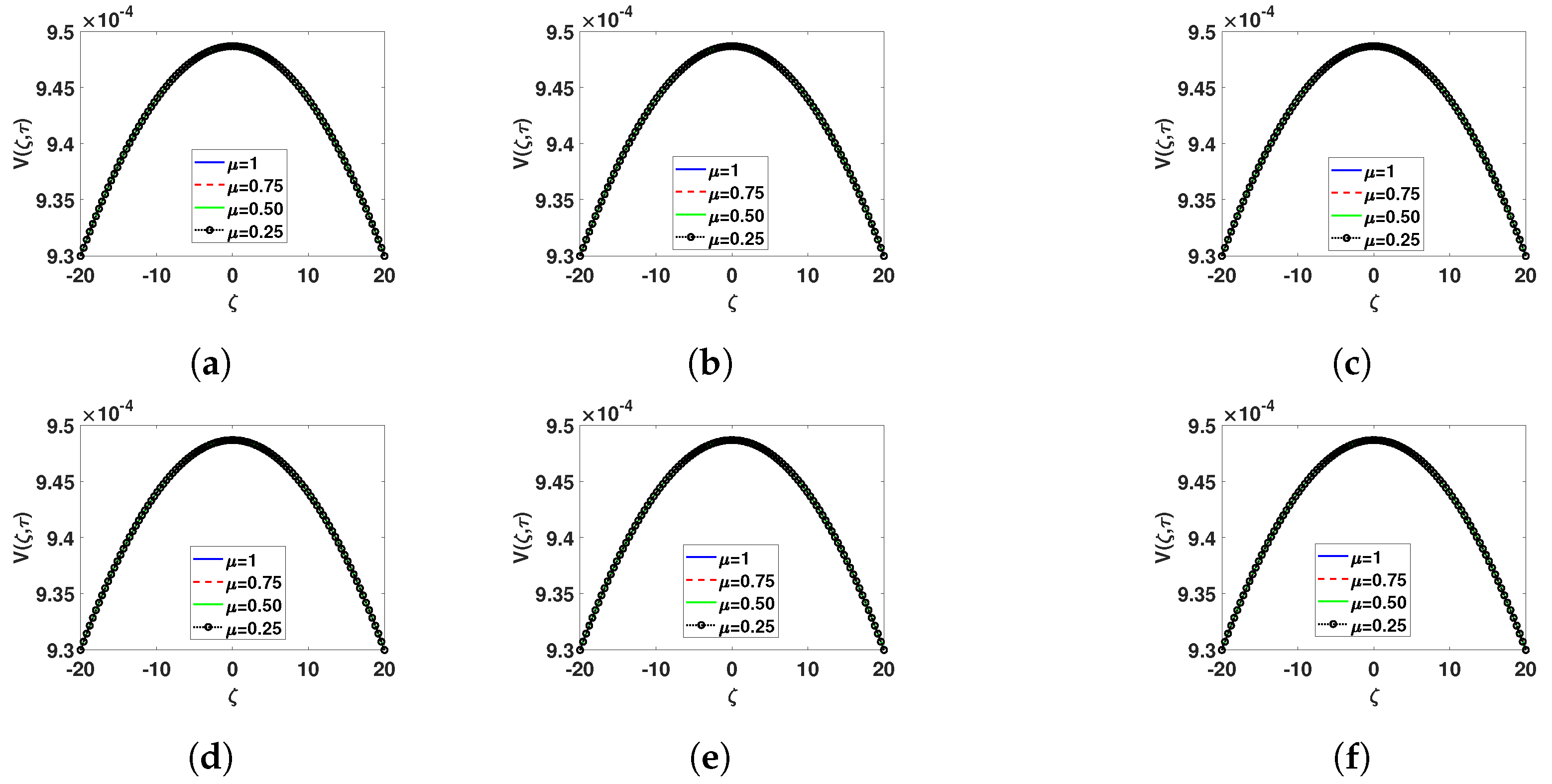
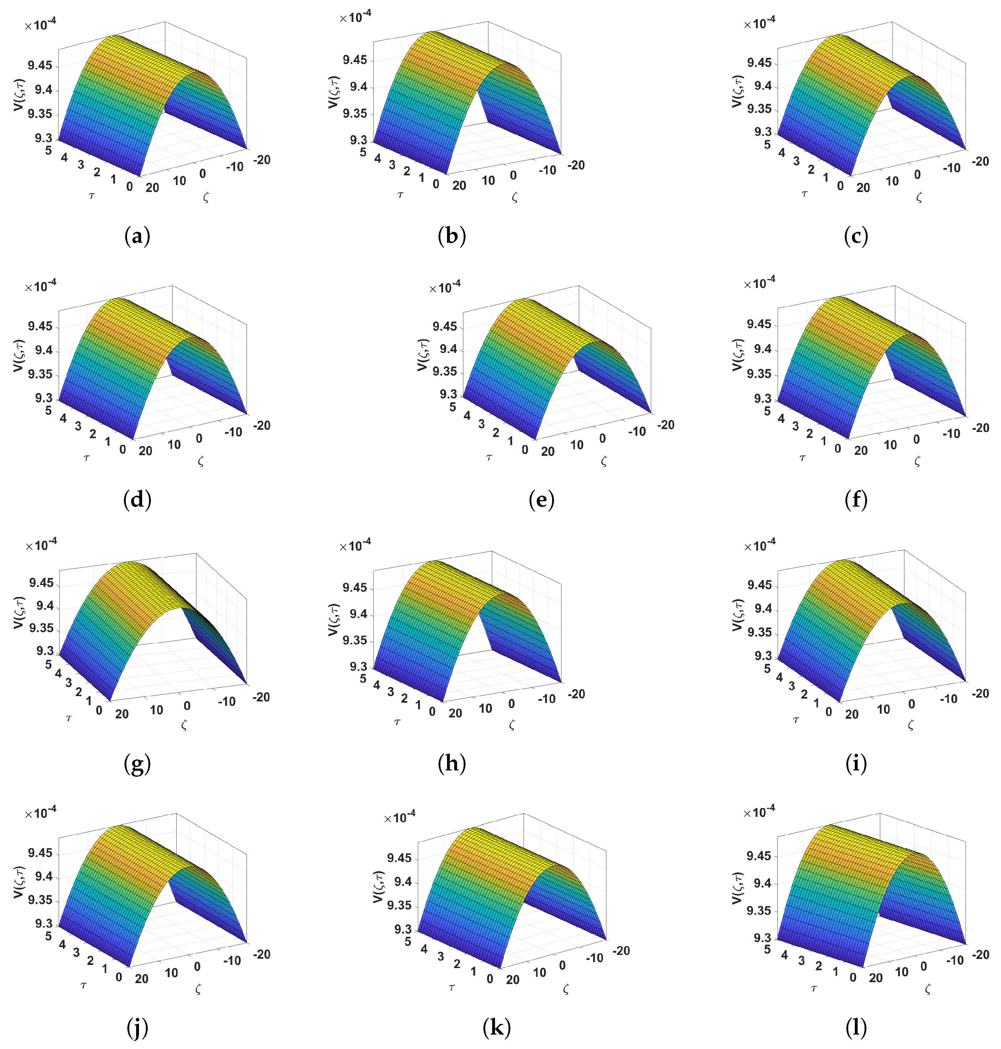
6. Numerical Results and Discussion

In this section, we illustrate the approximate solutions of TFKE and TFMKE using NTDM with unique space and time variables at various fractional-order values in Table 1, Table 2, Table 3 and Table 4. To demonstrate the dynamical behaviour of the solutions, their animations are exploited using numerical simulation in Figure 1, Figure 2, Figure 3 and Figure 4. Table 1 displays the absolute error of TFKE for various τ values at ζ = 10. Table 2 demonstrates the approximate solution of TFKE for various μ , τ values at fixed ζ = 10 using the current technique. Figure 1 shows the approximate solution of TFKE with different values of μ . Figure 2 shows the surface plot of the approximate solution of V ( ζ , τ ) with different values of μ . Table 3 displays the approximate solutions of TFMKE for various τ and ζ values at μ = 1 . Table 4 displays the approximate solution of TFMKE with various values of μ , τ , and ζ . Figure 3 shows the approximate solution of TFMKE with different values of μ . Figure 4 shows the surface plot of the approximate solution of V ( ζ , τ ) with different values of μ . The tables and graphs demonstrate the suggested techniques’ accuracy and applicability. From the figures, we can observe that three derivative graphical patterns are similar and symmetric. Tables display the accuracy of the proposed method with existing techniques with various fractional-order values.

7. Conclusions

In this work, we investigated the approximate solutions of TFKE and TFMKE based on the C, CF, and ABC fractional derivative operators using NTDM. The projected method is the amalgamation of two efficient techniques and it overcomes most of the limitations. The numerical simulation is shown to confirm the accuracy and to demonstrate that the fractional order goes to classical order. The derived solutions converge extremely fast to the actual solutions, indicating that approximate solutions are quite close to exact solutions. The numerical results suggest that the current technique is easy to use, effective, and precise. With the use of graphs and tables, the effect of all relevant parameters were discussed and presented. This is a fairly simple, dependable, and effective method for approximate solutions to several fractional physical models encountered in engineering and science such as the modified Korteweg–de Vries equation and it can also extended for fuzzy partial differential equations.

Author Contributions

P.K. contributed to the methodology, gathering the data, reading the manuscript, and visualisation, while R.K. contributed to investigation, validation, reading, writing up the manuscript, reviewing, and editing it, as well as supervising the work. All authors have read and agreed to the published version of the manuscript.

Funding

This study received no outside funding.

Institutional Review Board Statement

Not applicable.

Informed Consent Statement

Not applicable.

Data Availability Statement

Not applicable.

Acknowledgments

The authors would like to thank anonymous reviewers for their valuable suggestions to improve the manuscript in its present form. The authors extend their gratitude to Vellore Institute of Technology Vellore for providing the necessary facilities to carry out this work.

Conflicts of Interest

The authors declare no conflict of interest.

References

  1. Kaya, D.; Al-Khaled, K. A numerical comparison of a Kawahara equation. Phys. Lett. A 2007, 5–6, 433–439. [Google Scholar] [CrossRef]
  2. Lu, J. Analytical approach to Kawahara equation using variational iteration method and homotopy perturbation method. Topol. Methods Nonlinear Anal. 2008, 2, 287–293. [Google Scholar]
  3. Kudryashov, N.A. A note on new exact solutions for the Kawahara equation using Exp-function method. J. Comput. Appl. Math. 2010, 12, 3511–3512. [Google Scholar] [CrossRef]
  4. Kawahara, T. Oscillatory solitary waves in dispersive media. J. Phys. Soc. Jpn. 1972, 1, 260–264. [Google Scholar] [CrossRef]
  5. Jakub, V. Symmetries and conservation laws for a generalization of Kawahara equation. J. Geom. Phys. 2020, 150, 103579. [Google Scholar]
  6. Jin, L. Application of variational iteration method and homotopy perturbation method to the modified Kawahara equation. Math. Comput. Model Dyn. Syst. 2009, 3–4, 573–578. [Google Scholar] [CrossRef]
  7. Jabbari, A.; Kheiri, H. New exact traveling wave solutions for the Kawahara and modified Kawahara equations by using modified tanh-coth method. Acta Univ. Apulensis Math. Inform. 2010, 23, 21–38. [Google Scholar]
  8. Wazwaz, A.M. New solitary wave solutions to the modified Kawahara equation. Phys. Lett. A 2010, 4–5, 588–592. [Google Scholar] [CrossRef]
  9. Kurulay, M. Approximate analytic solutions of the modified Kawahara equation with homotopy analysis method. Adv. Differ. Equ. 2012, 2012, 178. [Google Scholar] [CrossRef]
  10. Miller, K.S.; Ross, B. An Introduction to the Fractional Calculus and Fractional Differential Equations; A Wiley-Interscience Publication; John Wiley & Sons, Inc.: New York, NY, USA, 1993. [Google Scholar]
  11. Podlubny, I. Fractional Differential Equations; Academic Press: New York, NY, USA, 1999. [Google Scholar]
  12. Hilfer, R. Applications of Fractional Calculus in Physics; World Scientific: Singapore, 2000. [Google Scholar]
  13. Herrmann, R. Fractional Calculus: An Introduction for Physicists; World Scientific: Singapore, 2011. [Google Scholar]
  14. Adomian, G. Solving Frontier Problems of Physics: The Decomposition Method; Springer Science and Business Media: Berlin/Heidelberg, Germany, 2013. [Google Scholar]
  15. Liu, P.; Din, A.; Zarin, R. Numerical dynamics and fractional modeling of hepatitis B virus model with non-singular and non-local kernels. Results Phys. 2022, 39, 105757. [Google Scholar] [CrossRef]
  16. Wu, P.; Din, A.; Munir, T.; Malik, M.Y.; Alqahtani, A.S. Local and global Hopf bifurcation analysis of an age-infection HIV dynamics model with cell-to-cell transmission. Waves Random Complex Media 2022. [Google Scholar] [CrossRef]
  17. Dhaigude, D.B.; Bhadgaonkar, V.N. A novel approach for fractional Kawahara and modified Kawahara equations using Atangana-Baleanu derivative operator. J. Math. Comput. Sci. 2021, 3, 2792–2813. [Google Scholar]
  18. Gaul, L.; Klein, P.; Kemple, S. Damping description involving fractional operators. Mech. Syst. Signal. Process. 1991, 2, 81–88. [Google Scholar] [CrossRef]
  19. de Oliveira, E.C.; Mainardi, F.; Vaz, J. Fractional models of anomalous relaxation based on the Kilbas and Saigo function. Meccanica 2014, 9, 2049–2060. [Google Scholar] [CrossRef]
  20. Figueiredo Camargo, R.; Capelas de Oliveira, E.; Vaz, J., Jr. On anomalous diffusion and the fractional generalized Langevin equation for a harmonic oscillator. J. Math. Phys. 2009, 12, 123518. [Google Scholar] [CrossRef]
  21. Langlands, T.A.M.; Henry, B.I.; Wearne, S.L. Fractional cable equation models for anomalous electrodiffusion in nerve cells: Infinite domain solutions. J. Math. Biol. 2009, 6, 761–808. [Google Scholar] [CrossRef]
  22. Abbasbandy, S. The application of homotopy analysis method to nonlinear equations arising in heat transfer. Phys. Lett. A 2006, 1, 109–113. [Google Scholar] [CrossRef]
  23. He, J.H. Variational iteration method–a kind of non-linear analytical technique: Some examples. Int. J. Non Linear Mech. 1999, 4, 699–708. [Google Scholar] [CrossRef]
  24. Sontakke, B.R.; Shelke, A.S.; Shaikh, A.S. Solution of non-linear fractional differential equations by variational iteration method and applications. Far East J. Math. Sci. 2019, 1, 113–129. [Google Scholar] [CrossRef]
  25. Dhaigude, D.B.; Kiwne, S.B.; Dhaigude, R.M. Monotone iterative scheme for weakly coupled system of finite difference reaction-diffusion equations. Commun. Appl. Anal. 2008, 2, 161. [Google Scholar]
  26. He, J.H. Homotopy perturbation technique. Comput. Methods Appl. Mech. Eng. 1999, 3–4, 257–262. [Google Scholar] [CrossRef]
  27. Inc, M.; Akgül, A.; Kiliçman, A. Explicit solution of telegraph equation based on reproducing kernel method. J. Funct. Spaces. Appl. 2012, 2012, 984682. [Google Scholar] [CrossRef]
  28. Boutarfa, B.; Akgül, A.; Inc, M. New approach for the Fornberg–Whitham type equations. J. Comput. Appl. Math. 2017, 312, 13–26. [Google Scholar] [CrossRef]
  29. Akgül, A. A novel method for a fractional derivative with non-local and non-singular kernel. Chaos Solit. Fractals. 2018, 114, 478–482. [Google Scholar] [CrossRef]
  30. Akgül, A.; Cordero, A.; Torregrosa, J.R. A fractional Newton method with 2αth-order of convergence and its stability. Appl. Math. Lett. 2019, 98, 344–351. [Google Scholar] [CrossRef]
  31. Seadawy, A.R.; Iqbal, M.; Lu, D. Propagation of kink and anti-kink wave solitons for the nonlinear damped modified Korteweg–de Vries equation arising in ion-acoustic wave in an unmagnetized collisional dusty plasma. Phys. Stat. Mech. Appl. 2020, 544, 123560. [Google Scholar] [CrossRef]
  32. Shah, K.; Seadawy, A.R.; Arfan, M. Evaluation of one dimensional fuzzy fractional partial differential equations. Alex. Eng. J. 2020, 59, 3347–3353. [Google Scholar] [CrossRef]
  33. Rahman, M.U.; Arfan, M.; Shah, Z.; Alzahrani, E. Evolution of fractional mathematical model for drinking under Atangana-Baleanu Caputo derivatives. Phys. Scr. 2021, 96, 115203. [Google Scholar] [CrossRef]
  34. Kiliç, S.Ş.Ş.; Çelik, E. Complex solutions to the higher-order nonlinear boussinesq type wave equation transform. Ric. Mat. 2022. [Google Scholar] [CrossRef]
  35. Yazgan, T.; Ilhan, E.; Çelik, E.; Bulut, H. On the new hyperbolic wave solutions to Wu-Zhang system models. Opt. Quantum Electron. 2022, 54, 298. [Google Scholar] [CrossRef]
  36. Tazgan, T.; Çelik, E.; Gülnur, Y.E.L.; Bulut, H. On Survey of the Some Wave Solutions of the Non-Linear Schrödinger Equation (NLSE) in Infinite Water Depth. Gazi Univ. J. Sci. 2022. [Google Scholar] [CrossRef]
  37. Rahman, M.U.; Arfan, M.; Deebani, W.; Kumam, P.; Shah, Z. Analysis of time-fractional Kawahara equation under Mittag-Leffler Power Law. Fractals 2022, 30, 2240021. [Google Scholar] [CrossRef]
  38. Zafar, H.; Ali, A.; Khan, K.; Sadiq, M.N. Analytical Solution of Time Fractional Kawahara and Modified Kawahara Equations by Homotopy Analysis Method. Int. J. Appl. Math. Comput. Sci. 2022, 8, 94. [Google Scholar] [CrossRef]
  39. Sontakke, B.R.; Shaikh, A. Approximate solutions of time fractional Kawahara and modified Kawahara equations by fractional complex transform. Commun. Numer. Anal. 2016, 2, 218–229. [Google Scholar] [CrossRef]
  40. Culha Ünal, S. Approximate Solutions of Time Fractional Kawahara Equation by Utilizing the Residual Power Series Method. Int. J. Appl. Math. Comput. Sci. 2022, 8, 78. [Google Scholar] [CrossRef]
  41. Mahmood, B.A.; Yousif, M.A. A novel analytical solution for the modified Kawahara equation using the residual power series method. Nonlinear Dyn. 2017, 89, 1233–1238. [Google Scholar] [CrossRef]
  42. Rawashdeh, M.S.; Maitama, S. Solving coupled system of nonlinear PDE’s using the natural decomposition method. Int. J. Pure Appl. Math. 2014, 5, 757–776. [Google Scholar] [CrossRef]
  43. Eltayeb, H.; Abdalla, Y.T.; Bachar, I.; Khabir, M.H. Fractional telegraph equation and its solution by natural transform decomposition method. Symmetry 2019, 3, 334. [Google Scholar] [CrossRef]
  44. Alrawashdeh, M.S.; Migdady, S. On finding exact and approximate solutions to fractional systems of ordinary differential equations using fractional natural adomian decomposition method. J. Algorithm Comput. Technol. 2022, 16. [Google Scholar] [CrossRef]
  45. Kanth, A.R.; Aruna, K.; Raghavendar, K.; Rezazadeh, H.; Inc, M. Numerical solutions of nonlinear time fractional Klein-Gordon equation via natural transform decomposition method and iterative Shehu transform method. J. Ocean Eng. Sci 2021. [Google Scholar] [CrossRef]
  46. Aljahdaly, N.H.; Agarwal, R.P.; Shah, R.; Botmart, T. Analysis of the time fractional-order coupled burgers equations with non-singular kernel operators. Mathematics 2021, 18, 2326. [Google Scholar] [CrossRef]
  47. Veeresha, P.; Prakasha, D.G.; Baskonus, H.M. Novel simulations to the time-fractional Fisher’s equation. Math. Sci. 2019, 1, 33–42. [Google Scholar] [CrossRef]
  48. Shah, N.A.; Hamed, Y.S.; Abualnaja, K.M.; Chung, J.D.; Shah, R.; Khan, A. A Comparative Analysis of Fractional-Order Kaup-Kupershmidt Equation within Different Operators. Symmetry 2022, 14, 986. [Google Scholar] [CrossRef]
  49. Saad Alshehry, A.; Imran, M.; Khan, A.; Shah, R.; Weera, W. Fractional View Analysis of Kuramoto-Sivashinsky Equations with Non-Singular Kernel Operators. Symmetry 2022, 14, 1463. [Google Scholar] [CrossRef]
  50. Caputo, M. Elasticita e Dissipazione; Zanichelli: Bologna, Italy, 1969. [Google Scholar]
  51. Losada, J.; Nieto, J.J. Properties of a new fractional derivative without singular kernel. Progr. Fract. Differ. Appl. 2015, 2, 87–92. [Google Scholar]
  52. Atangana, A.; Koca, I. Chaos in a simple nonlinear system with Atangana–Baleanu derivatives with fractional order. Chaos Solit. Fractals 2016, 89, 447–454. [Google Scholar] [CrossRef]
  53. Belgacem, F.B.M.; Silambarasan, R. Advances in the natural transform. AIP Conf. Proc. 2012, 1493, 106–110. [Google Scholar]
  54. Khan, Z.H.; Khan, W.A. N-transform properties and applications. NUST J. Eng. Sci. 2008, 1, 127–133. [Google Scholar]
  55. Loonker, D.; Banerji, P.K. Solution of fractional ordinary differential equations by natural transform. Int. J. Math. Eng. Sci. 2013, 2, 1–7. [Google Scholar]
  56. Khalouta, A.; Kadem, A. A new numerical technique for solving fractional Bratu’s initial value problems in the Caputo and Caputo-Fabrizio sense. J. Appl. Math. Comput. Mech. 2020, 1, 43–56. [Google Scholar] [CrossRef]
  57. Ravi Kanth, A.S.V.; Aruna, K.; Raghavendar, K. Numerical solutions of time fractional Sawada Kotera Ito equation via natural transform decomposition method with singular and nonsingular kernel derivatives. Math. Meth. Appl. Sci. 2021, 44, 14025–14040. [Google Scholar]
Figure 1. Approximate solution of Example 1 with different values μ . (a) NTDM C , τ = 5 ; (b) NTDM C F , τ = 5 ; (c) NTDM A B C , τ = 5 ; (d) NTDM C , τ = 10 ; (e) NTDM C F , τ = 10 ; (f) NTDM A B C , τ = 10 .
Symmetry 14 01777 g001
Figure 2. Surface plot of NTDM C , NTDM C F , NTDM A B C solution of V ( ζ , τ ) for Example 1 with different values of μ . (a) NTDM C , μ = 0.25 ; (b) NTDM C F , μ = 0.25 ; (c) NTDM A B C , μ = 0.25 ; (d) NTDM C , μ = 0.50 ; (e) NTDM C F , μ = 0.50 ; (f) NTDM A B C , μ = 0.50 ; (g) NTDM C , μ = 0.75 ; (h) NTDM C F , μ = 0.75 ; (i) NTDM A B C , μ = 0.75 ; (j) NTDM C , μ = 1 ; (k) NTDM C F , μ = 1 ; (l) NTDM A B C , μ = 1 .
Symmetry 14 01777 g002
Figure 3. Approximate solution of Example 2 with different values μ and a = 0.001 , b = 1 . (a) NTDM C , τ = 5 ; (b) NTDM C F , τ = 5 ; (c) NTDM A B C , τ = 5 ; (d) NTDM C , τ = 10 ; (e) NTDM C F , τ = 10 ; (f) NTDM A B C , τ = 10 .
Symmetry 14 01777 g003
Figure 4. Surface plot of NTDM C , NTDM C F , NTDM A B C solution of V ( ζ , τ ) for Example 2 with different values of μ with a = 0.001 , b = 1 . (a) NTDM C , μ = 0.25 ; (b) NTDM C F , μ = 0.25 ; (c) NTDM A B C , μ = 0.25 ; (d) NTDM C , μ = 0.50 ; (e) NTDM C F , μ = 0.50 ; (f) NTDM A B C , μ = 0.50 ; (g) NTDM C , μ = 0.75 ; (h) NTDM C F , μ = 0.75 ; (i) NTDM A B C , μ = 0.75 ; (j) NTDM C , μ = 1 ; (k) NTDM C F , μ = 1 ; (l) NTDM A B C , μ = 1 .
Symmetry 14 01777 g004
Table 1. Absolute error of TFKE in Example 1 with different values of τ at fixed ζ = 10 .
μ = 1
τ NTDM C NTDM CF NTDM ABC RPSM [40]
0.00000
0.11.41553 ×   10 15 1.41553 ×   10 15 1.41553 ×   10 15 1.41553 ×   10 15
0.24.68063 ×   10 14 4.68063 ×   10 14 4.68063 ×   10 14 4.68063 ×   10 14
0.33.6391 ×   10 13 3.6391 ×   10 13 3.6391 ×   10 13 3.6391 ×   10 13
0.41.56886 ×   10 12 1.56886 ×   10 12 1.56886 ×   10 12 1.56886 ×   10 12
0.54.89617 ×   10 12 4.89617 ×   10 12 4.89617 ×   10 12 4.89617 ×   10 12
0.61.24542 ×   10 11 1.24542 ×   10 11 1.24542 ×   10 11 1.24542 ×   10 11
0.72.75069 ×   10 11 2.75069 ×   10 11 2.75069 ×   10 11 2.75069 ×   10 11
0.85.47829 ×   10 11 5.47829 ×   10 11 5.47829 ×   10 11 5.47829 ×   10 11
0.91.0081 ×   10 10 1.0081 ×   10 10 1.0081 ×   10 10 1.0081 ×   10 10
1.01.7428 ×   10 10 1.7428 ×   10 10 1.7428 ×   10 10 1.7428 ×   10 10
Table 2. Approximate solution of TFKE in Example 1 with different values of μ , τ at fixed ζ = 10 .
μ = 0.25
τ NTDM C NTDM CF NTDM ABC RPSM [40]
0.03.04206 ×   10 2 3.29806 ×   10 2 3.29806 ×   10 2 3.04206 ×   10 2
0.13.25021 ×   10 2 3.30723 ×   10 2 3.35567 ×   10 2 3.25033 ×   10 2
0.23.29225 ×   10 2 3.31643 ×   10 2 3.36675 ×   10 2 3.29247 ×   10 2
0.33.32093 ×   10 2 3.32564 ×   10 2 3.37421 ×   10 2 3.32123 ×   10 2
0.43.34339 ×   10 2 3.33488 ×   10 2 3.38000 ×   10 2 3.34378 ×   10 2
0.53.36214 ×   10 2 3.34414 ×   10 2 3.38480 ×   10 2 3.3626 ×   10 2
0.63.37839 ×   10 2 3.35342 ×   10 2 3.38893 ×   10 2 3.37893 ×   10 2
0.83.40585 ×   10 2 3.37206 ×   10 2 3.39586 ×   10 2 3.40655 ×   10 2
0.93.41778 ×   10 2 3.38141 ×   10 2 3.39885 ×   10 2 3.41855 ×   10 2
1.03.42882 ×   10 2 3.39078 ×   10 2 3.40160 ×   10 2 3.42966 ×   10 2
0.03.04206 ×   10 2 3.20859 ×   10 2 3.20859 ×   10 2 3.04206 ×   10 2
0.13.15837 ×   10 2 3.22610 ×   10 2 3.27177 ×   10 2 3.15838 ×   10 2
0.23.20842 ×   10 2 3.24370 ×   10 2 3.29844 ×   10 2 3.20845 ×   10 2
0.33.24759 ×   10 2 3.26138 ×   10 2 3.31911 ×   10 2 3.24765 ×   10 2
0.43.28114 ×   10 2 3.27915 ×   10 2 3.33667 ×   10 2 3.28122 ×   10 2
0.53.31109 ×   10 2 3.29700 ×   10 2 3.35224 ×   10 2 3.31122 ×   10 2
0.63.33850 ×   10 2 3.31495 ×   10 2 3.36641 ×   10 2 3.33867 ×   10 2
0.73.36398 ×   10 2 3.33297 ×   10 2 3.37950 ×   10 2 3.36421 ×   10 2
0.83.38794 ×   10 2 3.35109 ×   10 2 3.39175 ×   10 2 3.38822 ×   10 2
0.93.41066 ×   10 2 3.36929 ×   10 2 3.40331 ×   10 2 3.41099 ×   10 2
1.03.43233 ×   10 2 3.38757 ×   10 2 3.41429 ×   10 2 3.43273 ×   10 2
μ = 0.75
0.03.04206 ×   10 2 3.12331 ×   10 2 3.12331 ×   10 2 3.04206 ×   10 2
0.13.10417 ×   10 2 3.14837 ×   10 2 3.17206 ×   10 2 3.10417 ×   10 2
0.23.14737 ×   10 2 3.17362 ×   10 2 3.20580 ×   10 2 3.14737 ×   10 2
0.33.18582 ×   10 2 3.19905 ×   10 2 3.23572 ×   10 2 3.18583 ×   10 2
0.43.22162 ×   10 2 3.22466 ×   10 2 3.26348 ×   10 2 3.22163 ×   10 2
0.53.25565 ×   10 2 3.25047 ×   10 2 3.28978 ×   10 2 3.25567 ×   10 2
0.63.28839 ×   10 2 3.27645 ×   10 2 3.31501 ×   10 2 3.28842 ×   10 2
0.73.32014 ×   10 2 3.30263 ×   10 2 3.33941 ×   10 2 3.32019 ×   10 2
0.83.35111 ×   10 2 3.32900 ×   10 2 3.36315 ×   10 2 3.35117 ×   10 2
0.93.38144 ×   10 2 3.35556 ×   10 2 3.38633 ×   10 2 3.38153 ×   10 2
1.03.41124 ×   10 2 3.38231 ×   10 2 3.40906 ×   10 2 3.41135 ×   10 2
μ = 1
0.03.04206 ×   10 2 3.04206 ×   10 2 3.04206 ×   10 2 3.04206 ×   10 2
0.13.07393 ×   10 2 3.07393 ×   10 2 3.07393 ×   10 2 3.07393 ×   10 2
0.23.10612 ×   10 2 3.10612 ×   10 2 3.10612 ×   10 2 3.10612 ×   10 2
0.33.13861 ×   10 2 3.13861 ×   10 2 3.13861 ×   10 2 3.13861 ×   10 2
0.43.17143 ×   10 2 3.17143 ×   10 2 3.17143 ×   10 2 3.17143 ×   10 2
0.53.20455 ×   10 2 3.20455 ×   10 2 3.20455 ×   10 2 3.20455 ×   10 2
0.63.23800 ×   10 2 3.23800 ×   10 2 3.23800 ×   10 2 3.23800 ×   10 2
0.73.27178 ×   10 2 3.27178 ×   10 2 3.27178 ×   10 2 3.27178 ×   10 2
0.83.30588 ×   10 2 3.30588 ×   10 2 3.30588 ×   10 2 3.30588 ×   10 2
0.93.34030 ×   10 2 3.34030 ×   10 2 3.34030 ×   10 2 3.34030 ×   10 2
1.03.37506 ×   10 2 3.37506 ×   10 2 3.37506 ×   10 2 3.37506 ×   10 2
Table 3. Approximate solution of TFMKE in Example 2 with different values of ζ , τ with a = 0.001 , b = 1 .
μ = 1
ζ τ NTDM C NTDM CF NTDM ABC HAM [38]
−200.09.2996 ×   10 4 9.2996 ×   10 4 9.2996 ×   10 4 9.299 ×   10 4
0.29.2996 ×   10 4 9.2996 ×   10 4 9.2996 ×   10 4 9.299 ×   10 4
0.49.2996 ×   10 4 9.2996 ×   10 4 9.2996 ×   10 4 9.299 ×   10 4
0.69.2996 ×   10 4 9.2996 ×   10 4 9.2996 ×   10 4 9.299 ×   10 4
0.89.2996 ×   10 4 9.2996 ×   10 4 9.2996 ×   10 4 9.299 ×   10 4
1.09.2996 ×   10 4 9.2996 ×   10 4 9.2996 ×   10 4 9.299 ×   10 4
−100.09.4396 ×   10 4 9.4396 ×   10 4 9.4396 ×   10 4 9.439 ×   10 4
0.29.4396 ×   10 4 9.4396 ×   10 4 9.4396 ×   10 4 9.439 ×   10 4
0.49.4396 ×   10 4 9.4396 ×   10 4 9.4396 ×   10 4 9.439 ×   10 4
0.69.4396 ×   10 4 9.4396 ×   10 4 9.4396 ×   10 4 9.439 ×   10 4
0.89.4396 ×   10 4 9.4396 ×   10 4 9.4396 ×   10 4 9.439 ×   10 4
1.09.4396 ×   10 4 9.4396 ×   10 4 9.4396 ×   10 4 9.439 ×   10 4
00.09.4868 ×   10 4 9.4868 ×   10 4 9.4868 ×   10 4 9.486 ×   10 4
0.29.4868 ×   10 4 9.4868 ×   10 4 9.4868 ×   10 4 9.486 ×   10 4
0.49.4868 ×   10 4 9.4868 ×   10 4 9.4868 ×   10 4 9.486 ×   10 4
0.69.4868 ×   10 4 9.4868 ×   10 4 9.4868 ×   10 4 9.486 ×   10 4
0.89.4868 ×   10 4 9.4868 ×   10 4 9.4868 ×   10 4 9.486 ×   10 4
1.09.4868 ×   10 4 9.4868 ×   10 4 9.4868 ×   10 4 9.486 ×   10 4
100.09.4396 ×   10 4 9.4396 ×   10 4 9.4396 ×   10 4 9.439 ×   10 4
0.29.4396 ×   10 4 9.4396 ×   10 4 9.4396 ×   10 4 9.439 ×   10 4
0.49.4396 ×   10 4 9.4396 ×   10 4 9.4396 ×   10 4 9.439 ×   10 4
0.69.4396 ×   10 4 9.4396 ×   10 4 9.4396 ×   10 4 9.439 ×   10 4
0.89.4396 ×   10 4 9.4396 ×   10 4 9.4396 ×   10 4 9.439 ×   10 4
1.09.4396 ×   10 4 9.4396 ×   10 4 9.4396 ×   10 4 9.439 ×   10 4
200.09.2996 ×   10 4 9.2996 ×   10 4 9.2996 ×   10 4 9.299 ×   10 4
0.29.2996 ×   10 4 9.2996 ×   10 4 9.2996 ×   10 4 9.299 ×   10 4
0.49.2996 ×   10 4 9.2996 ×   10 4 9.2996 ×   10 4 9.299 ×   10 4
0.69.2996 ×   10 4 9.2996 ×   10 4 9.2996 ×   10 4 9.299 ×   10 4
0.89.2996 ×   10 4 9.2996 ×   10 4 9.2996 ×   10 4 9.299 ×   10 4
1.09.2996 ×   10 4 9.2996 ×   10 4 9.2996 ×   10 4 9.299 ×   10 4
Table 4. Approximate solution of TFMKE in Example 2 with different values of μ , τ and ζ with a = 0.001 , b = 1 .
ζ τ μ = 0.25 μ = 0.50 μ = 0.75
NTDM C NTDM CF NTDM ABC NTDM C NTDM CF NTDM ABC NTDM C NTDM CF NTDM ABC
−200.09.2996 ×   10 4 9.2996 ×   10 4 9.2996 ×   10 4 9.2996 ×   10 4 9.2996 ×   10 4 9.2996 ×   10 4 9.2996 ×   10 4 9.2996 ×   10 4 9.2996 ×   10 4
0.29.2996 ×   10 4 9.2996 ×   10 4 9.2996 ×   10 4 9.2996 ×   10 4 9.2996 ×   10 4 9.2996 ×   10 4 9.2996 ×   10 4 9.2996 ×   10 4 9.2996 ×   10 4
0.49.2996 ×   10 4 9.2996 ×   10 4 9.2996 ×   10 4 9.2996 ×   10 4 9.2996 ×   10 4 9.2996 ×   10 4 9.2996 ×   10 4 9.2996 ×   10 4 9.2996 ×   10 4
0.69.2996 ×   10 4 9.2996 ×   10 4 9.2996 ×   10 4 9.2996 ×   10 4 9.2996 ×   10 4 9.2996 ×   10 4 9.2996 ×   10 4 9.2996 ×   10 4 9.2996 ×   10 4
0.89.2996 ×   10 4 9.2996 ×   10 4 9.2996 ×   10 4 9.2996 ×   10 4 9.2996 ×   10 4 9.2996 ×   10 4 9.2996 ×   10 4 9.2996 ×   10 4 9.2996 ×   10 4
1.09.2996 ×   10 4 9.2996 ×   10 4 9.2996 ×   10 4 9.2996 ×   10 4 9.2996 ×   10 4 9.2996 ×   10 4 9.2996 ×   10 4 9.2996 ×   10 4 9.2996 ×   10 4
−100.09.4396 ×   10 4 9.4396 ×   10 4 9.4396 ×   10 4 9.4396 ×   10 4 9.4396 ×   10 4 9.4396 ×   10 4 9.4396 ×   10 4 9.4396 ×   10 4 9.4396 ×   10 4
0.29.4396 ×   10 4 9.4396 ×   10 4 9.4396 ×   10 4 9.4396 ×   10 4 9.4396 ×   10 4 9.4396 ×   10 4 9.4396 ×   10 4 9.4396 ×   10 4 9.4396 ×   10 4
0.49.4396 ×   10 4 9.4396 ×   10 4 9.4396 ×   10 4 9.4396 ×   10 4 9.4396 ×   10 4 9.4396 ×   10 4 9.4396 ×   10 4 9.4396 ×   10 4 9.4396 ×   10 4
0.69.4396 ×   10 4 9.4396 ×   10 4 9.4396 ×   10 4 9.4396 ×   10 4 9.4396 ×   10 4 9.4396 ×   10 4 9.4396 ×   10 4 9.4396 ×   10 4 9.4396 ×   10 4
0.89.4396 ×   10 4 9.4396 ×   10 4 9.4396 ×   10 4 9.4396 ×   10 4 9.4396 ×   10 4 9.4396 ×   10 4 9.4396 ×   10 4 9.4396 ×   10 4 9.4396 ×   10 4
1.09.4396 ×   10 4 9.4396 ×   10 4 9.4396 ×   10 4 9.4396 ×   10 4 9.4396 ×   10 4 9.4396 ×   10 4 9.4396 ×   10 4 9.4396 ×   10 4 9.4396 ×   10 4
00.09.4868 ×   10 4 9.4868 ×   10 4 9.4868 ×   10 4 9.4868 ×   10 4 9.4868 ×   10 4 9.4868 ×   10 4 9.4868 ×   10 4 9.4868 ×   10 4 9.4868 ×   10 4
0.29.4868 ×   10 4 9.4868 ×   10 4 9.4868 ×   10 4 9.4868 ×   10 4 9.4868 ×   10 4 9.4868 ×   10 4 9.4868 ×   10 4 9.4868 ×   10 4 9.4868 ×   10 4
0.49.4868 ×   10 4 9.4868 ×   10 4 9.4868 ×   10 4 9.4868 ×   10 4 9.4868 ×   10 4 9.4868 ×   10 4 9.4868 ×   10 4 9.4868 ×   10 4 9.4868 ×   10 4
0.69.4868 ×   10 4 9.4868 ×   10 4 9.4868 ×   10 4 9.4868 ×   10 4 9.4868 ×   10 4 9.4868 ×   10 4 9.4868 ×   10 4 9.4868 ×   10 4 9.4868 ×   10 4
0.89.4868 ×   10 4 9.4868 ×   10 4 9.4868 ×   10 4 9.4868 ×   10 4 9.4868 ×   10 4 9.4868 ×   10 4 9.4868 ×   10 4 9.4868 ×   10 4 9.4868 ×   10 4
1.09.4868 ×   10 4 9.4868 ×   10 4 9.4868 ×   10 4 9.4868 ×   10 4 9.4868 ×   10 4 9.4868 ×   10 4 9.4868 ×   10 4 9.4868 ×   10 4 9.4868 ×   10 4
100.09.4396 ×   10 4 9.4396 ×   10 4 9.4396 ×   10 4 9.4396 ×   10 4 9.4396 ×   10 4 9.4396 ×   10 4 9.4396 ×   10 4 9.4396 ×   10 4 9.4396 ×   10 4
0.29.4396 ×   10 4 9.4396 ×   10 4 9.4396 ×   10 4 9.4396 ×   10 4 9.4396 ×   10 4 9.4396 ×   10 4 9.4396 ×   10 4 9.4396 ×   10 4 9.4396 ×   10 4
0.49.4396 ×   10 4 9.4396 ×   10 4 9.4396 ×   10 4 9.4396 ×   10 4 9.4396 ×   10 4 9.4396 ×   10 4 9.4396 ×   10 4 9.4396 ×   10 4 9.4396 ×   10 4
0.69.4396 ×   10 4 9.4396 ×   10 4 9.4396 ×   10 4 9.4396 ×   10 4 9.4396 ×   10 4 9.4396 ×   10 4 9.4396 ×   10 4 9.4396 ×   10 4 9.4396 ×   10 4
0.89.4396 ×   10 4 9.4396 ×   10 4 9.4396 ×   10 4 9.4396 ×   10 4 9.4396 ×   10 4 9.4396 ×   10 4 9.4396 ×   10 4 9.4396 ×   10 4 9.4396 ×   10 4
1.09.4396 ×   10 4 9.4396 ×   10 4 9.4396 ×   10 4 9.4396 ×   10 4 9.4396 ×   10 4 9.4396 ×   10 4 9.4396 ×   10 4 9.4396 ×   10 4 9.4396 ×   10 4
200.09.2996 ×   10 4 9.2996 ×   10 4 9.2996 ×   10 4 9.2996 ×   10 4 9.2996 ×   10 4 9.2996 ×   10 4 9.2996 ×   10 4 9.2996 ×   10 4 9.2996 ×   10 4
0.29.2996 ×   10 4 9.2996 ×   10 4 9.2996 ×   10 4 9.2996 ×   10 4 9.2996 ×   10 4 9.2996 ×   10 4 9.2996 ×   10 4 9.2996 ×   10 4 9.2996 ×   10 4
0.49.2996 ×   10 4 9.2996 ×   10 4 9.2996 ×   10 4 9.2996 ×   10 4 9.2996 ×   10 4 9.2996 ×   10 4 9.2996 ×   10 4 9.2996 ×   10 4 9.2996 ×   10 4
0.69.2996 ×   10 4 9.2996 ×   10 4 9.2996 ×   10 4 9.2996 ×   10 4 9.2996 ×   10 4 9.2996 ×   10 4 9.2996 ×   10 4 9.2996 ×   10 4 9.2996 ×   10 4
0.89.2996 ×   10 4 9.2996 ×   10 4 9.2996 ×   10 4 9.2996 ×   10 4 9.2996 ×   10 4 9.2996 ×   10 4 9.2996 ×   10 4 9.2996 ×   10 4 9.2996 ×   10 4
1.09.2996 ×   10 4 9.2996 ×   10 4 9.2996 ×   10 4 9.2996 ×   10 4 9.2996 ×   10 4 9.2996 ×   10 4 9.2996 ×   10 4 9.2996 ×   10 4 9.2996 ×   10 4
Publisher’s Note: MDPI stays neutral with regard to jurisdictional claims in published maps and institutional affiliations.

