Abstract
Aiming at the conversion process of thrust vectoring vertical/short takeoff and landing (V/STOL) aircraft with a symmetrical structure in the transition stage of takeoff and landing, there is a problem with the coupling and redundancy of the control quantities. To solve this problem, a corresponding inner loop stabilization controller and control distribution strategy are designed. In this paper, a dynamic system model and a dynamic model are established. Based on the outer loop adopting the conventional nonlinear dynamic inverse control, an L1 adaptive controller is designed based on the model as the inner loop stabilization control to compensate the mismatch and uncertainty in the system. The key feature of the L1 adaptive control architecture is ensuring robustness in the presence of fast adaptation, so as to achieve a unified performance boundary in transient and steady-state operations, thus eliminating the need for adaptive rate gain scheduling. The control performance and robustness of the controller are verified by inner loop simulation and the shooting Monte Carlo approach. The simulation results show that the controller can still track the reference input well and has good robustness when there is a large parameter perturbation.
1. Introduction
Thrust vectoring technology can directly change the thrust magnitude and thrust direction of aircraft, which is an important technical scheme to achieve the high maneuverability of modern aircraft. Unlike conventional fighter jets, vertical/short takeoff and landing (V/STOL) aircraft is a new type of aircraft [1,2,3]. It can not only realize the vertical takeoff and landing, but also carry out a high-speed cruise in a conventional aircraft configuration and will be widely used in the military field in the future. Therefore, the thrust vectoring vehicle has the characteristics of a large flight space, complex flight action, and diverse flight tasks, resulting in the strong nonlinearity of its control system and severe changes in the external environment. How to design a control scheme that can deal with this large uncertainty is a key problem in the control design of a thrust vectoring vehicle.
Regarding the aspect of mathematical model establishment and simulation, Songlin Ma and Weijun Wang [4] established a longitudinal model in a transition flight phase for a new concept of vertical/short takeoff and landing aircraft. Xiaomeng Zhang and Weijun Wang [5] analyzed the dynamics of the vertical/short takeoff and landing of unmanned aerial UAVs and obtained a nonlinear dynamics model. References [6,7] investigated the thrust vector control of thrust vectoring V/STOL aircraft using a six-degree-of-freedom flight dynamics simulation. For controller design, Yang, Xili et al. [8] proposed two nonlinear approaches for the autonomous transition control of two vertical/short takeoff and landing aircraft. Walker, G. and Allen, D. [9] presented an overview of the X-35B control law requirements, design, analysis, and summary of the STOVL flight test results. In Reference [10], a control scheme comprising the dynamic characteristics of the thrust vectoring system was developed for V/STOL aircraft. Simulation and experimental results were presented. Zhiqiang Cheng et al. [11] proposed an optimal trajectory transition controller. Reference [12] showed an application of L1 adaptive control theory for the attitude control of UAVs. Chiang R Y, et al. [13] presented an H-∞ flight control system design case study for a supermaneuverable fighter flying quality of the Herbst maneuver, which may provide some reference for hovering state flying quality. Zian, Wang et al. [14] used an L1 adaptive inner loop controller and designed a roll-horizon landing deceleration and landing strategy for hybrid-wing vehicles. Seshagiri S, et al. [15] considered the application of a conditional integrator-based sliding mode control design for robust regulation of minimum-phase nonlinear systems for the control of the longitudinal flight dynamics of an F-16 aircraft. Liu, N, et al. [16] used the nonlinear active disturbance rejection controller (ADRC) to control the tilt wings. In terms of control allocation, Min, B.M, et al. [17] focused on applying various control allocation schemes to the SAT-II UAV system. Tan J, et al. [18] studied attitude tracking UAVs with the terminal sliding mode based on the extended state observer and with the multi-objective nonlinear control allocation. For the problem of simulation verification, References [19,20] provided a practical Monte Carlo method to verify the robustness of the controller.
In the transition stage of the thrust vectoring V/STOL aircraft, the tilt angle of the vectoring nozzle and the opening of the lift fan will change greatly. In this power conversion process, both the aerodynamic rudder surface and the power system of the aircraft can control the six degrees of freedom of the aircraft. At this stage, the aircraft will face the problems of strong nonlinearity, control quantity coupling, and redundancy. The design of the control law is a great challenge. Under the physical constraints of the thrust vectoring vehicle, the aerodynamic control inputs and thrust vectoring control inputs are allocated according to the virtual control variables. To solve this problem, based on the F35B scale model, the dynamic equation modeling is given in this paper. On this basis, the inner loop controller and control distribution method are designed. Finally, the performance and robustness of the controller are verified by inner loop simulation and the shooting Monte Carlo approach.
The remainder of this paper is organized as follows. Section 2 introduces the composition of the thrust vector V/STOL aircraft power system and establishes the dynamic equation modeling by combining the whole vehicle dynamics equation, kinematic equation, and moment equation. Section 3 introduces the design of the inner loop and outer loop controllers in detail, and the control allocation method is given. The robustness of the inner loop controller is simulated and verified by Monte Carlo simulation in Section 4, and conclusions and recommendations for future work are stated in Section 5
2. Dynamic Equation Modeling
The thrust vectoring vertical/short takeoff and landing aircraft used in this paper is a self-made F35B scale model with a total weight of about 13 kg, a cruising speed of 30 m/s, and a cruising altitude of less than 100 m.
The F35B consists of a fuselage, wings, tail, and power system as shown in Figure 1. The F35B mainly has the fixed-wing mode and vertical takeoff and landing (VTOL) mode. The platform’s aerodynamic control surfaces include a full-motion horizontal tail, a full-motion vertical tail, and flaperons. The power system consists of two subsystems: the lift fan and auxiliary motor subsystem installed in the front section of the fuselage; the main ducted fan and the main motor subsystem installed in the rear section of the fuselage; a three-bearing swivel duct (3BSD) nozzle is connected behind the main ducted fan.
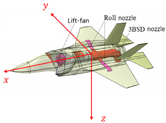
Figure 1.
F35 model.
2.1. Whole Vehicle Dynamics Model
We use to denote the thrust components of the engine under the three shafts. The aerodynamic force is defined in the airflow coordinate system, and considering the lift loss in the transition section, the total aerodynamic force can be expressed as Equation (1), where is the drag force, C is the side force, and is the lift force.
The direction of the aircraft’s gravity is given in the z-axis of the ground coordinate system, which is also converted to the airframe coordinate system.
Combined with Equations (1) and (2), the linear motion equation of the aircraft in the body coordinate system can be determined from Equation (3).
where are the velocity components of the three coordinate axes in the body coordinate system and are roll angle velocity, pitch angle velocity, and yaw angle velocity in the body coordinate system, respectively.
2.2. Kinematic Equations and Moment Equation
The kinematic equations and moment equation of the aircraft are [9]:
where are the roll angle, pitch angle, and yaw angle of the aircraft, respectively; are the moment equation coefficients; are roll moment, pitch moment, and yaw moment in the body coordinate system, respectively.
Based on Equations (3)–(5), the nonlinear dynamics model of the aircraft can be derived:
3. L1 Stabilization Controller Design
The stability augmentation controller in this paper constitutes a control and stability augmentation system (CSAS) by controlling the roll, pitch, and yaw of the aircraft. The CSAS can generate angular velocity and acceleration control commands and provides torque commands to the control distributor. Then, a single-input single-output (SISO) L1 adaptive controller is designed for each of the three angular velocity channels to compensate for mismatch uncertainties in the dynamics [21,22,23]. For outer-loop designs such as pitch and roll, nonlinear dynamic inversion (NDI) provides the tracking of the required dynamics. Figure 2 shows the adaptive control flow diagram using NDI and the L1 adaptive control law.
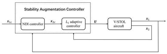
Figure 2.
Flow chart of L1 adaptive controller.
In Figure 2, the outer loop state variable and the inner loop state variable ; the control inputs of the V/STOL aircraft are ; are the aileron deflection, elevator deflection, and rudder deflection, respectively; is the ratio of the lift fan thrust to the maximal lift fan thrust; is the ratio between the maximum three-bearing swivel duct nozzle thrust and the three-bearing swivel duct nozzle thrust; is the three-bearing swivel duct nozzle’s pitch angle, when the aircraft is in fixed-wing mode, , and in vertical takeoff and landing mode, ; is the yaw angle of the three-bearing swivel duct nozzle, as shown in Figure 3; are the thrust of the left and right roll nozzles, respectively. The actuator characteristics are described in Table 1.
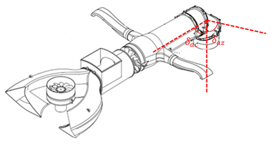
Figure 3.
Power system diagram.

Table 1.
Effector characteristics of the F35B.
The pitch and roll channels realize the decoupling of the angle and angular velocity according to the timescale separation principle. The attitude angle is controlled by the NDI method, while the L1 adaptive controller controls the angular velocity. The L1 adaptive law can be divided into four parts: control object, state predictor, adaptive law, and control law.
3.1. Inner Loop Controller Design
3.1.1. NDI Controller Design of Roll Loop
First, the NDI controller needs to be designed for the roll loop. The kinematic equation of the outer loop is:
where , are affine functions satisfying and .
The error is defined as . Based on the NDI method, the angular velocity command can be obtained:
where is the bandwidth coefficient and is a diagonal matrix, which is determined by the flight quality of the aircraft and the outer loop bandwidth.
3.1.2. L1 Adaptive Controller Design of Roll Angular Velocity Loop
According to the small perturbation theory, the kinematic equation of the outer loop Equation (7) can be simplified as
where is the virtual angular acceleration, are the aerodynamic coefficients, and are the virtual control torque generated by the virtual output signal . can be solved by Equation (9) and expressed as:
where and are the roll angular accelerations generated by the air surface and the vector nozzle, respectively. At low airspeeds, the control torque provided by the vectoring nozzle dominates. The vector nozzle provides the required pitch acceleration, i.e., , . At high airspeeds, the aerodynamic surfaces subject to the required pitch angular acceleration, i.e., , . During the transitional flight, both the aerodynamic surfaces and the vectoring nozzle achieve the commanded roll angular acceleration.
Considering the uncertainty of moment, Equation (9) can be expressed as:
where are the uncertain aerodynamic factors and is the disturbance factor. The structure of the first-order reference model is as follows:
Combining Equations (9)–(12), we can write the control model of the rolling loop as:
where is the feedback gain matrix, is the virtual control factor, is the aerodynamic factor, and is the aerodynamic disturbance.
Three assumptions and a lemma are given.
Assumption 1.
The unknown constant is uniformly bounded, i.e.,, is a compact convex set.
Assumption 2.
is uniformly bounded in Equation (19), such as , b > 0, where is the -norm.
Assumption 3.
The partial derivatives of are semi-globally uniformly bounded: for , there exist and independent of time to ensure that the partial derivatives of are piecewise continuous and bounded, as follows:
The assumptions can be met since the uncertainty for the inner loop control system is of a given magnitude.
Lemma 1.
For τ > 0, if and , where and are positive constants, and are continuous. Furthermore, their derivatives with respect to are:
where and are computable finite values; is the -norm.
Based on the above assumptions and lemma, an adaptive law controller is designed, which consists of a state predictor, an adaptive law, and a control law:
- State predictor:
According to Equation (13), the state predictor can be expressed as:
where is the predicted level of control factor uncertainty, is the expected degree of the aerodynamic factor’s uncertainty, and is the predicted degree of the aerodynamic disturbance’s uncertainty; denotes the estimated level of control factor uncertainty, B the estimated level of aerodynamic factor uncertainty, and C the estimated level of aerodynamic disturbance uncertainty.
- Law of adaptation:
- Control law:
The control law is as follows:
where is the adaptive feedback gain, is the low-pass filter, and is the adaptive feedforward gain. The L1 adaptive control scheme is shown in Figure 3. Control laws should be designed to ensure that the following transfer functions are strictly regular:
where satisfies and is a 3 × 3 identity matrix.
When obtaining and , the following conditions must be satisfied to ensure the stability of adaptive control:
where , , , and are defined as:
where is an arbitrary positive number.
In the case of satisfying Equation (20), The adaptive controller of the inner loop consists of Equations (16)–(18). The block diagram of the adaptive controller system is shown in Figure 4.
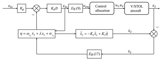
Figure 4.
Adaptive controller system block diagram.
3.2. Control Allocation
Equation (6) can be expressed as:
where are the system state variables, are the system control variables, and , .
Expanding Equation (22) by Taylor series at the equilibrium point, keeping the linear part, and ignoring the high-order part, we can obtain:
where is the system state matrix, which consists of the partial derivatives of forces and moments with respect to the state variables. is the control derivative matrix, which is the aerodynamic change generated by the unit control amount, which can reflect the control efficiency of the aircraft by the control input. The subscript trim indicates the trim value. System control variables can be solved by Equation (23).
4. Inner Loop Controller Simulation Experiment
According to the inner loop controller and control distribution method designed in the previous section, the simulation verification results are given in this section. The difficulty in controlling the V/STOL aircraft is that there is a flight mode conversion process during the takeoff and landing process. At this stage, the two sets of control mechanisms of the aircraft are involved in the work of jointly controlling the position and attitude of the aircraft. Therefore, in this state, the working point is selected for inner loop simulation and the shooting Monte Carlo approach to verify the performance of the inner loop stabilization controller and control distribution method designed in this paper.
4.1. Monte Carlo Targeting at Nominal State
An L1 controller with and receives a 5°/s frequent square roll rate command as the input. Figure 5 and Figure 6 show the outcomes for various combinations of and .
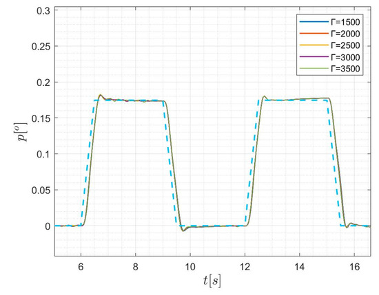
Figure 5.
Roll rate command tracking results at Kp = 8.
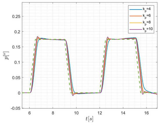
Figure 6.
Roll rate command tracking results at Γ = 2500.
We settled on and as the virtual control coefficient and virtual state coefficient, respectively, because they strike a balance between speed and stability, have a brief risetime, and exhibit zero overshoots.
According to the inner loop controller designed in the previous section, in fixed–wing mode, set the height to 25 m and the airspeed to 24 m/s. In this state, given step signals for the roll and pitch angles, the simulation results are shown in Figure 7.
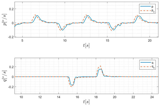
Figure 7.
Roll rate and pitch rate command tracking results in fixed-wing mode.
It can be seen from the figure that this controller can track the pitch angle command well; the adjustment time of the inner loop pitch angle and roll angle command is about 1 s, and there is no obvious overshoot.
In VTOL mode, set the height to 25 m and the airspeed to 16 m/s. In this state, given step signals for the roll and pitch angles, the simulation results are shown in Figure 8:
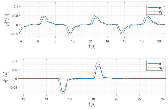
Figure 8.
Roll rate and pitch rate command tracking results in VTOL mode.
The findings reveal that the curve’s shape is the same in both modes, and the L1 controller’s tracking performance is superb with a steady-state error of zero and a minor temporal lag.
4.2. Target Shooting Monte Carlo Approach in Level Flight
The robustness of the inner loop controller was simulated and verified by Monte Carlo simulation. Its parameter perturbation variables mainly include aerodynamic characteristics, mass characteristics, and the dynamic system. The change of perturbation parameters is shown in Table 2.
Table 2.
Main parameters of the V/STOL vehicle.
are the control derivatives; are the stability derivatives; are the damping derivatives; are the cross-damping derivatives; are the inertia moments.
The above parameters are randomly changed, and the shooting Monte Carlo approach is performed on the aircraft in constant level flight and acceleration conditions, respectively. At an altitude of 100 m, the aircraft is in constant level flight at a speed of 20 m/s. At 15 s, a 10° pitch angle command is given to conduct a target shooting Monte Carlo approach simulation test. Then, comparing it with the PID controller [24,25,26], the simulation results are shown in Figure 9, Figure 10, Figure 11, Figure 12 and Figure 13.
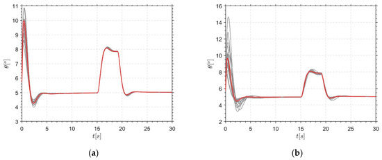
Figure 9.
The shooting Monte Carlo approach at the pitch angle. (a) L1 adaptive controller; (b) PID controller.
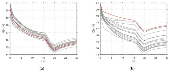
Figure 10.
The shooting Monte Carlo approach at the airspeed; (a) L1 adaptive controller; (b) PID controller.
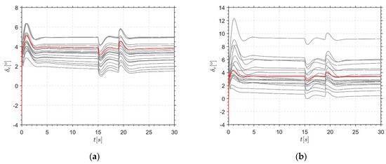
Figure 11.
The target shooting Monte Carlo approach with the elevator; (a) L1 adaptive controller; (b) PID controller.
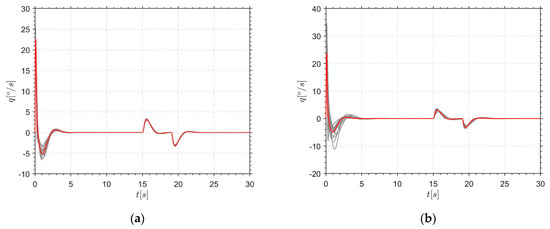
Figure 12.
The shooting Monte Carlo approach at the pitch angle velocity; (a) L1 adaptive controller; (b) PID controller.
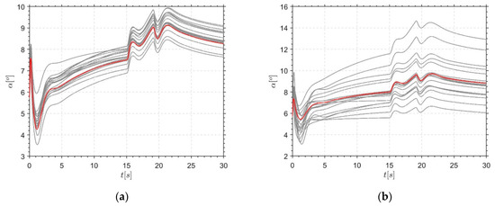
Figure 13.
The shooting Monte Carlo approach at the angle of attack; (a) L1 adaptive controller; (b) PID controller.
As can be seen from the above figure, the control channels of each direction of the aircraft are decoupled. The controller designed in this paper is obviously better than the PID controller for instruction tracking. This shows that the controller designed in this paper can still track the command well and has good robustness under the premise that the parameters of the aircraft are taken.
5. Conclusions
Based on the conventional nonlinear dynamic inverse control of the outer loop, an L1 adaptive controller was designed as the inner loop stability augmentation control to compensate the uncertainty in the system. The expected verification results were obtained from the Monte Carlo simulations. The main contributions of this paper are as follows:
- (1)
- This paper introduced the composition of the power system of the thrust vectoring V/STOL aircraft and established the dynamic equation of the F35B scale model prototype.
- (2)
- For the thrust vector V/STOL aircraft with strong coupling and nonlinearity, based on the conventional dynamic inverse control in the outer loop, an L1 adaptive stabilization controller was designed on the inner loop to compensate for the mismatch uncertainty. The designed control structure integrates the fixed-wing mode and the VTOL mode.
- (3)
- The uncertainty of modeling and possible input disturbances were fully considered and compared with the PID controller. It was verified by simulation that the controller quickly responds to the command and has good robustness when there is a large parameter perturbation.
Author Contributions
Conceptualization, Z.G. and Z.Z.; methodology, Z.G.; software, Z.G. and Z.Z.; validation, Z.Z. and Z.G.; formal analysis, Z.Z. and Z.W.; investigation, Z.W.; resources, X.Z.; data curation, Z.W.; writing—original draft preparation, Z.G. and Z.Z.; writing—review and editing, Z.W. and Z.Z.; visualization, Y.Y.; supervision, Z.W.; project administration, P.C. All authors have read and agreed to the published version of the manuscript.
Funding
This research received no external funding.
Data Availability Statement
Data available on request due to restrictions eg privacy or ethical. The data presented in this study are available on request from the corresponding author. The data are not publicly available due to commercial use.
Conflicts of Interest
The authors declare no conflict of interest.
References
- Su, W.; Gao, Z.H.; Xia, L. Multiobjective optimization design of aerodynamic configuration constrained by stealth performance. Acta Aerodyn. Sin. 2006, 24, 137–140. [Google Scholar]
- Jacobson, S.; Britt, R.; Freim, D.; Kelly, P. Residual pitch oscillation (rpo) flight test and analysis on the b-2 bomber. ICES J. Mar. Sci. 2003, 67, 1260–1271. [Google Scholar]
- Britt, R.T.; Arthurs, T.D.; Jacobson, S.B. Aeroservoelastic analysis of the B-2 bomber. J. Aircr. 2000, 37, 745–752. [Google Scholar] [CrossRef]
- Ma, S.; Wang, W. The Longitudinal Modeling of a New Concept V/STOL UAV in Transition Flight by Using the Method of System Identification. In Proceedings of the 2018 10th International Conference on Intelligent Human-Machine Systems and Cybernetics (IHMSC), Hangzhou, China, 25–26 August 2018. [Google Scholar]
- Zhang, X.; Wang, W. Dynamic modelling of the hovering phase of a new V/STOL UAV and verification of the PID control strategy. IOP Conf. Ser. Mater. Sci. Eng. 2018, 408, 12–17. [Google Scholar] [CrossRef]
- Wang, X.; Zhu, J.; Zhang, Y. Dynamics modeling and analysis of thrust-vectored V/STOL aircraft. In Proceedings of the 32nd Chinese Control Conference, IEEE, Xi’an, China, 26–28 July 2013. [Google Scholar]
- Nagabhushan, B.L.; Faiss, G.D. Thrust vector control of a v/stol airship. J. Aircr. 1984, 21, 408–413. [Google Scholar] [CrossRef]
- Yang, X.; Fan, Y.; Zhu, J. Transition flight control of two vertical/short takeoff and landing aircraft. J. Guid. Control. Dyn. 2008, 31, 371–385. [Google Scholar]
- Walker, G.; Allen, D. X-35B STOVL Flight Control Law Design and Flying Qualities. In Proceedings of the 2002 Biennial International Powered Lift Conference and Exhibit, Williamsburg, VA, USA, 5–7 November 2002. [Google Scholar]
- Wang, X.; Zhu, B.; Zhu, J.; Cheng, Z. Thrust vectoring control of vertical/short takeoff and landing aircraft. Sci. China 2020, 63, 218–220. [Google Scholar] [CrossRef]
- Cheng, Z.; Zhu, J.; Yuan, X.; Wang, X. Design of optimal trajectory transition controller for thrust-vectored v/stol aircraft. Sci. China Inf. Sci. 2021, 64, 139201. [Google Scholar] [CrossRef]
- Mallikarjunan, S.; Nesbitt, B.; Kharisov, E. L1 adaptive controller for attitude control of multirotors. In Proceedings of the Guidance, Navigation, and Control Conference, Minneapolis, MN, USA, 13–16 August 2012. [Google Scholar]
- Chiang, R.Y.; Safonov, M.G.; Haiges, K.; Madden, K.; Tekawy, J. A fixed H∞ controller for a supermaneuverable fighter performing the herbst maneuver. Automatic 1993, 29, 111. [Google Scholar] [CrossRef]
- Wang, Z.; Mao, S.; Gong, Z.; Zhang, C.; He, J. Energy Efficiency Enhanced Landing Strategy for Manned eVTOLs Using L1 Adaptive Control. Symmetry 2021, 13, 21–25. [Google Scholar] [CrossRef]
- Seshagiri, S.; Promtun, E. Sliding mode control of F-16 longitudinal dynamics. In Proceedings of the 2008 American Control Conference, Seattle, WA, USA, 11–13 June 2008. [Google Scholar]
- Liu, N.; Cai, Z.; Wang, Y. Fast level-flight to hover mode transition and altitude control in tiltrotor’s landing operation. Chin. J. Aeronaut. 2020, 34, 181–193. [Google Scholar] [CrossRef]
- Min, B.M.; Kim, E.T.; Tahk, M.J. Application of Control Allocation Methods to SAT-II UAV. In Proceedings of the Aiaa Guidance, Navigation, & Control Conference & Exhibit, San Francisco, CA, USA, 15–18 August 2005. [Google Scholar]
- Tan, J.; Zhou, Z.; Zhu, X.; Xu, M. Attitude control of flying wing uav based on terminal sliding mode and control allocation. J. Northwestern Polytech. Univ. 2014, 32, 505–510. [Google Scholar]
- Shakarian, A. Application of Monte-Carlo Techniques to the 757/767 Autoland Dispersion Analysis by Simulation. Guid. Control Conf. 1983, 83, 181–194. [Google Scholar]
- Chao, Z.; Chen, L.; Chen, Z. Monte Carlo Simulation for Vision-based Autonomous Landing of Unmanned Combat Aerial Vehicles. J. Syst. Simul. 2010, 22, 2235–2240. [Google Scholar]
- Xargay, E.; Hovakimyan, N.; Dobrokhodov, V.; Statnikov, R.; Kaminer, I.; Cao, C.; Gregory, I. L1 Adaptive Flight Control System: Systematic Design and Verification and Validation of Control Metrics. In Proceedings of the AIAA Guidance, Navigation, and Control Conference, Toronto, ON, Canada, 2–5 August 2010. [Google Scholar]
- Leman, T.; Xargay, E.; Dullerud, G.; Hovakimyan, N.; Wendel, T. L1 Adaptive Control Augmentation System for the X-48b AircrafAIA Guidance. In Proceedings of the Navigation, and Control Conference, Chicago, IL, USA, 10–13 August 2009; AIAA, Urbana-Champaign: Champaign, IL, USA, 2009. [Google Scholar]
- Jiang, G.; Liu, G.; Yu, H. A Model Free Adaptive Scheme for Integrated Control of Civil Aircraft Trajectory and Attitude. Symmetry 2021, 13, 347. [Google Scholar] [CrossRef]
- Faruk, T.; Ali, A.; Naim, A.; Firas, A.; Basil Al, K.; Özyavaş, A. Robust Nonlinear Non-Referenced Inertial Frame Multi-Stage PID Controller for Symmetrical Structured UAV. Symmetry 2022, 14, 689. [Google Scholar] [CrossRef]
- Ma, J.; Xie, H.; Song, K.; Liu, H. Self-Optimizing Path Tracking Controller for Intelligent Vehicles Based on Reinforcement Learning. Symmetry 2022, 14, 31. [Google Scholar] [CrossRef]
- Zhong, C.Q.; Wang, L.; Xu, C.F. Path Tracking of Permanent Magnet Synchronous Motor Using Fractional Order Fuzzy PID Controller. Symmetry 2021, 13, 1118. [Google Scholar] [CrossRef]


Publisher’s Note: MDPI stays neutral with regard to jurisdictional claims in published maps and institutional affiliations. |
© 2022 by the authors. Licensee MDPI, Basel, Switzerland. This article is an open access article distributed under the terms and conditions of the Creative Commons Attribution (CC BY) license (https://creativecommons.org/licenses/by/4.0/).