Abstract
Stochastic partial differential equations have wide applications in various fields of science and engineering. This paper addresses the optical stochastic solitons and other exact stochastic solutions through birefringent fibers for the Biswas–Arshed equation with multiplicative white noise using the modified extended mapping method. This model contains many kinds of soliton solutions, which are always symmetric or anti-symmetric in space. Stochastic bright soliton solutions, stochastic dark soliton solutions, stochastic combo bright–dark soliton solutions, stochastic combo singular-bright soliton solutions, stochastic singular soliton solutions, stochastic periodic solutions, stochastic rational solutions, stochastic Weierstrass elliptic doubly periodic solutions, and stochastic Jacobi elliptic function solutions are extracted. The constraints on the parameters are considered to guarantee the existence of these stochastic solutions. Furthermore, some of the selected solutions are described graphically to demonstrate the physical nature of the obtained solutions.
1. Introduction
The noise arising in physics, telecommunication networks, hydrology, medicine, and so on can be modeled by stochastic partial differential equations. One of the important research directions of stochastic partial differential equations is the stochastic wave, which has been studied by many authors (see [1,2,3]). Optical solitons are used to transmit very large amounts of data at the speed of light without error and loss over very long distances (see [4,5,6,7,8,9,10,11,12,13,14,15,16,17,18,19,20,21,22,23,24,25,26,27,28,29,30,31]. However, some natural conditions cause stochastic distortions in communication. Noise cannot be ignored because its effects will lead to distortions and significant consequences. For this reason, it is important to establish differential equations with stochastic terms so that the established models can be more precise. Subsequently, the solitary wave solutions of nonlinear stochastic partial differential equations (NSPDEs) are always symmetric or anti-symmetric in space. Some of the literature discusses the stochastic soliton solutions of NSPDEs, for example, Khan et al. [32] studied the stochastic perturbation of optical solitons with anti-cubic nonlinearity with bandpass filters and multi-photon absorption. He and Wang [33] obtained dark multi-soliton and soliton molecule solutions of the stochastic nonlinear Schrödinger equation in the white noise space. Arshed et al. [34] studied the chiral solitons of the (2+1)-dimensional stochastic chiral nonlinear Schrödinger equation. Secer [35] investigated the stochastic optical solitons with multiplicative white noise via Itô calculus. Yin et al. [36] discussed the stochastic soliton solutions for the (2+1)-dimensional stochastic Broer–Kaup equations in a fluid or plasma. Zayed et al. [37] extracted optical solitons in birefringent fibers with the Biswas–Arshed equation with multiplicative noise via Itô calculus using the extended simplest equation algorithm and the Jacobi elliptic expansion approach. Saleh et al. [38] discussed Lie symmetry analysis of stochastic gene evolution in a double-chain deoxyribonucleic acid system.
In the present study, we consider the Biswas–Arshed equation with multiplicative white noise in the Itô sense in the following form [37]:
where the complex-valued functions are denoted by and , and are the coefficients of chromatic dispersion, and are the coefficients of spatio-temporal dispersion, and are the coefficients of third-order dispersion, and and are the coefficients of third-order spatio-temporal dispersion. and are the coefficients of the noise strength and and are the standard Wiener processes, such that and are the white noise. and are the coefficients of self-steepening. The coefficients of the nonlinear dispersion terms are represented by .
In this paper, the modified extended mapping method is presented for the proposed model to obtain stochastic optical solitons through birefringent fibers and other stochastic exact solutions. The presented method gives a variety of solutions and the stochastic bright soliton solutions, stochastic dark soliton solutions, stochastic combo bright–dark soliton solutions, stochastic combo singular-bright soliton solutions, stochastic singular soliton solutions, stochastic periodic solutions, stochastic rational solutions, stochastic Weierstrass elliptic doubly periodic solutions, and stochastic Jacobi elliptic function solutions are extracted. Our motivation is to improve the work of [37] by giving many new solutions that can help in the field of telecommunications for coding or the transmission of data. When we compare our results and those obtained in [37] using the extended simplest equation algorithm and the Jacobi elliptic expansion approach, we observe that there are many new solutions in the present work. Moreover, some of the obtained stochastic solutions are represented graphically.
2. Preliminaries
In this section, the modified extended mapping method is presented briefly [39,40]. Assume the following nonlinear partial differential equation:
Suppose that Equation (3) has a traveling wave solution of the form:
Then, Equation (3) is reduced to the following nonlinear ordinary differential equation:
We suppose that Equation (5) has a solution of the following form:
where ,,, and are constants, and achieves the following equation:
where are constants.
Through Equation (5), the positive integer N is found by balancing the highest-order nonlinear terms and the highest-order derivatives.
Solution (6) is substituted into Equation (5) with the auxiliary Equation (7). Then, the coefficients of the same powers are summed and set equal to zero, then, we obtain a system of algebraic equations that can be solved by Mathematica or Maple to obtain the unknown constants ,,, , and ℑ. Thus, we obtain the exact solutions of Equation (3).
3. Stochastic Solitons and Other Solutions
In order to obtain the stochastic solutions of (1) and (2), we use the following wave transformations:
and
The amplitude portions of the solitons are represented by , whereas the phase components of the solitons are represented by , and the frequencies, wave numbers, and velocities of the solitons are represented by , and ℑ, respectively.
When compensating from Equations (8)–(10) into Equations (1) and (2), with the separation of the real and imaginary parts, we obtain:
Set
where T is a non-zero constant. Then, Equations (11)–(14) convert to
By integrating Equations (18) and (19), under the special choice of the integration constant as zero, we obtain:
When applying the linearly independent principle to Equations (20) and (21), we obtain the speed and wave numbers of the solitons as:
and
with
Then, Equations (16) and (17) are equivalent under the constraints:
In addition, Equation (16) can be represented as follows:
where
According to the modified extended mapping method, the solution for Equation (28) can be expressed as follows:
where and are constants, which we can set under the restrictions or or .
Insert Equations (29) and (7) into Equation (28) and then collect the coefficients of the same powers and set them equal to zero. This yields a system of algebraic equations that can be solved using Mathematica software. Then, the following cases are obtained:
- Case 1:
- .
- Set 1:
- Set 2:
- Set 3:
- (1.1,1)
- If , then,represent bright solitons.
- (1.1,2)
- If , then,orrepresent singular periodic wave solutions.
- (1.1,3)
- If then,represent rational solutions.
- (1.2,1)
- If , then,represent dark solitons.
- (1.2,2)
- If , then,orrepresent periodic wave solutions.
- (1.2,3)
- If then,represent rational solutions.
Through set 3, if , then,
represent combo bright–dark solitons.
- Case 2:
- .
- Set 1:
- Set 2:
- Set 3:
- Set 4:
- Set 5:
- Set 6:
- Set 7:
- (2.1,1)
- If , then,represent dark solitons.
- (2.1,2)
- If then,represent periodic solutions.
- (2.2,1)
- If , then,represent singular solitons.
- (2.2,2)
- If then,represent periodic solutions.
- (2.3,1)
- If , then,represent singular solitons.
- (2.3,2)
- If then,represent periodic solutions.
- (2.4,1)
- If , then,represent singular solitons.
- (2.2,2)
- If then,represent periodic solutions.
- (2.5,1)
- If , then,represent singular solitons.
- (2.5,2)
- If then,represent periodic solutions.
- (2.6,1)
- If , then,represent singular solitons.
- (2.6,2)
- If then,represent periodic solutions.
Through set 7, if , then,
- represent periodic solutions.
- Case 3:
- If, we set ,
- (3.1)
- If , then,represent combo singular-bright solitons.
- (3.2)
- If then,represent periodic solutions.
- (3.3)
- If then,represent periodic solutions.
- Case 4:
- If we set ,
Then,
represent stochastic rational solutions with
- Case 5:
- .
- Set 1:
- Set 2:
- Set 3:
- Set 4:
- (5.1,1)
- If , then,represent dark solitons.
- (5.1,2)
- If , then,represent singular solitons.
- (5.2,1)
- If , then,represent singular solitons.
- (5.2,2)
- If , thenrepresent combo bright–dark solitons.
- (5.3,1)
- If , then,represent singular solitons.
- (5.3,2)
- If , then,represent periodic solutions.
- (5.4,1)
- If , then,represent singular solitons.
- (5.4,2)
- If , then,represent periodic solutions.
- Case 6:
- If we set ,
Then,
represent stochastic Weierstrass elliptic doubly periodic solutions with
- Case 7:
- .
- Set 1:
- Set 2:
- Set 3:
- (7.1,1)
- If , then,orrepresent Jacobi elliptic function solutions.If we take , then,orrepresent periodic solutions.
- (7.1,2)
- If , then,represent Jacobi elliptic function solutions.If we take , then,represent dark solitons.
- (7.1,3)
- If , then,If we take , then,represent dark solitons.
- (7.1,4)
- If , then,represent Jacobi elliptic function solutions.
- (7.2,1)
- If then,orrepresent periodic solutions.
- (7.2,2)
- If , then,represent dark solitons.
- (7.3,1)
- If then,represent periodic solutions.
- (7.3,2)
- If , then,represent dark solitons.
4. Graphic Illustration
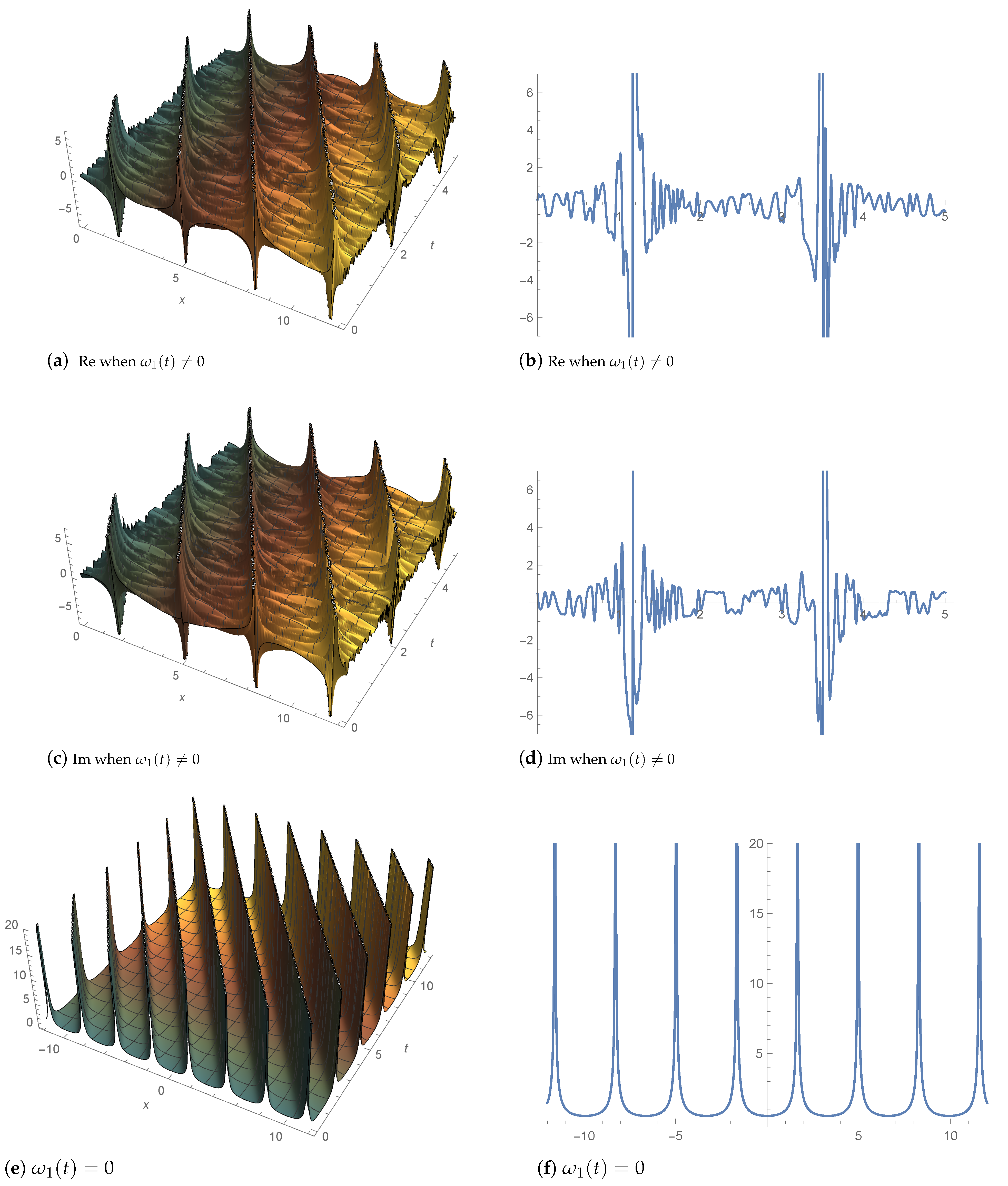
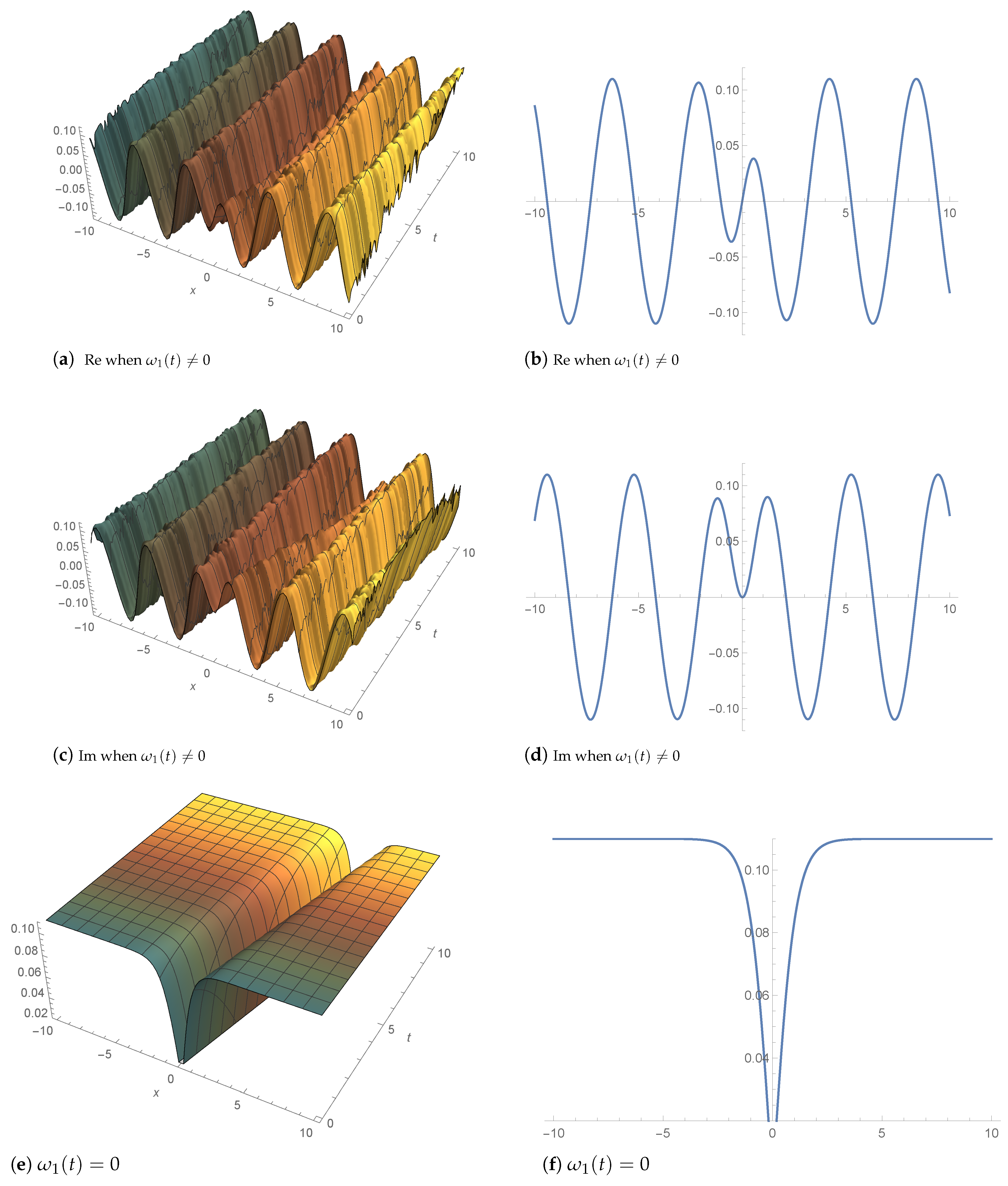
In this part, the numerical simulations of some of the solutions are illustrated as follows. Figure 1 represents the bright soliton solution of Equation (30). The values of the selected parameters are . Figure 2 represents the singular periodic wave solutions of Equation (32). The values of the selected parameters are . Figure 3 represents the dark soliton solution of Equation (38). The values of the selected parameters are . Figure 4 represents the singular soliton solution of Equation (64). The values of the selected parameters are .
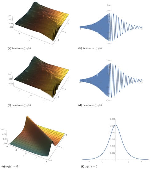
Figure 1.
Equation (30): 3D and 2D illustrations.
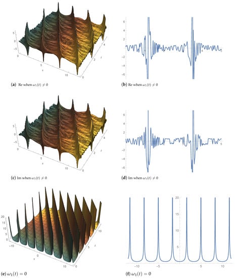
Figure 2.
Equation (32): 3D and 2D illustrations.

Figure 3.
Equation (38): 3D and 2D illustrations.
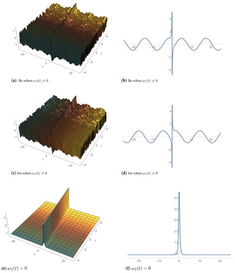
Figure 4.
Equation (64): 3D and 2D illustrations.
5. Conclusions
In our paper, the Biswas–Arshed equation with multiplicative white noise has been studied successfully using the modified extended mapping method. Various types of stochastic solutions were obtained such as stochastic bright soliton solutions, stochastic dark soliton solutions, stochastic combo bright–dark soliton solutions, stochastic combo singular-bright soliton solutions, stochastic singular soliton solutions, stochastic periodic solutions, stochastic rational solutions, stochastic Weierstrass elliptic doubly periodic solutions, and stochastic Jacobi elliptic function solutions. The constraints on the parameters were considered to guarantee the existence of the obtained solutions. By comparing our results with the outcomes of [37], it has been recognized that the stochastic dark soliton solutions, stochastic combo bright–dark soliton solutions, stochastic combo singular-bright soliton solutions, periodic solutions, rational solutions, and Weierstrass elliptic doubly periodic solutions have been obtained for the first time in this article. Moreover, 3D plots with contour plots of some solutions were introduced to show their features. Moreover, for the physical illustration of the obtained stochastic solutions, the movements of some of the achieved solutions were described graphically (Figure 1, Figure 2, Figure 3 and Figure 4).
Author Contributions
Conceptualization, Y.A. and H.M.A.; methodology, W.B.R.; software, W.B.R.; validation, Y.A., H.M.A. and W.B.R.; formal analysis, H.M.A.; investigation, Y.A.; resources, W.B.R.; writing—original draft preparation, Y.A.; writing—review and editing, H.M.A.; supervision, H.M.A.; funding acquisition, Y.A. All authors have read and agreed to the published version of the manuscript.
Funding
The APC was funded by the Deanship of Scientific Research, Qassim University.
Data Availability Statement
Not applicable.
Acknowledgments
The researchers would like to thank the Deanship of Scientific Research, Qassim University, for funding the publication of this project.
Conflicts of Interest
The authors declare no conflict of interest.
References
- Hyder, A.A.; Soliman, A.H. Analytical manner for abundant stochastic wave solutions of extended KdV equation with conformable differential operators. Math. Methods Appl. Sci. 2022, 45, 8600–8612. [Google Scholar] [CrossRef]
- Abdelrahman, M.A.; Sohaly, M.A. On the new wave solutions to the MCH equation. Indian J. Phys. 2019, 93, 903–911. [Google Scholar] [CrossRef]
- Oh, T.; Okamoto, M. Comparing the stochastic nonlinear wave and heat equations: A case study. Electron. J. Probab. 2021, 26, 1–44. [Google Scholar] [CrossRef]
- Kudryashov, N.A. Stationary solitons of the generalized nonlinear Schrödinger equation with nonlinear dispersion and arbitrary refractive index. Appl. Math. Lett. 2022, 128, 107888. [Google Scholar] [CrossRef]
- Ahmed, K.K.; Badra, N.M.; Ahmed, H.M.; Rabie, W.B. Soliton Solutions and Other Solutions for Kundu–Eckhaus Equation with Quintic Nonlinearity and Raman Effect Using the Improved Modified Extended Tanh-Function Method. Mathematics 2022, 10, 4203. [Google Scholar] [CrossRef]
- Bekir, A.; Zahran, E. Three distinct and impressive visions for the soliton solutions to the higher-order nonlinear Schrodinger equation. Optik 2021, 228, 166157. [Google Scholar] [CrossRef]
- Arshad, M.; Seadawy, A.R.; Lu, D. Modulation stability and dispersive optical soliton solutions of higher order nonlinear Schrödinger equation and its applications in mono-mode optical fibers. Superlattices Microstruct. 2018, 113, 419–429. [Google Scholar] [CrossRef]
- Rasheed, N.M.; Al-Amr, M.O.; Az-Zo’bi, E.A.; Tashtoush, M.A.; Akinyemi, L. Stable optical solitons for the Higher-order Non-Kerr NLSE via the modified simple equation method. Mathematics 2021, 9, 1986. [Google Scholar] [CrossRef]
- Kudryashov, N.A. Optical solitons of the generalized nonlinear Schrödinger equation with Kerr nonlinearity and dispersion of unrestricted order. Mathematics 2022, 10, 3409. [Google Scholar] [CrossRef]
- Hendi, A.A.; Ouahid, L.; Kumar, S.; Owyed, S.; Abdou, M.A. Dynamical behaviors of various optical soliton solutions for the Fokas–Lenells equation. Mod. Phys. Lett. B 2021, 35, 2150529. [Google Scholar] [CrossRef]
- Ozisik, M. On the optical soliton solution of the (1+1)-dimensional perturbed NLSE in optical nano-fibers. Optik 2022, 250, 168233. [Google Scholar] [CrossRef]
- Tozar, A.; Tasbozan, O.; Kurt, A. Optical soliton solutions for the (1+1)-dimensional resonant nonlinear Schröndinger’s equation arising in optical fibers. Opt. Quantum Electron. 2021, 53, 316. [Google Scholar] [CrossRef]
- Hosseini, K.; Mirzazadeh, M.; Gómez-Aguilar, J.F. Soliton solutions of the Sasa–Satsuma equation in the monomode optical fibers including the beta-derivatives. Optik 2020, 224, 165425. [Google Scholar] [CrossRef]
- Owyed, S.; Abdou, M.A.; Abdel-Aty, A.H.; Ray, S.S. New optical soliton solutions of nolinear evolution equation describing nonlinear dispersion. Commun. Theor. Phys. 2019, 71, 1063. [Google Scholar] [CrossRef]
- Younis, M.; Seadawy, A.R.; Baber, M.Z.; Husain, S.; Iqbal, M.S.; Rizvi, S.T.R.; Baleanu, D. Analytical optical soliton solutions of the Schrödinger-Poisson dynamical system. Results Phys. 2021, 27, 104369. [Google Scholar] [CrossRef]
- Ali, K.K.; Wazwaz, A.M.; Osman, M.S. Optical soliton solutions to the generalized nonautonomous nonlinear Schrödinger equations in optical fibers via the sine-Gordon expansion method. Optik 2020, 208, 164132. [Google Scholar] [CrossRef]
- Rabie, W.B.; Seadawy, A.R.; Ahmed, H.M. Highly dispersive Optical solitons to the generalized third-order nonlinear Schrödinger dynamical equation with applications. Optik 2021, 241, 167109. [Google Scholar] [CrossRef]
- Bilal, M.; Ren, J.; Younas, U. Stability analysis and optical soliton solutions to the nonlinear Schrödinger model with efficient computational techniques. Opt. Quantum Electron. 2021, 53, 406. [Google Scholar] [CrossRef]
- Rezazadeh, H.; Ullah, N.; Akinyemi, L.; Shah, A.; Mirhosseini-Alizamin, S.M.; Chu, Y.M.; Ahmad, H. Optical soliton solutions of the generalized non-autonomous nonlinear Schrödinger equations by the new Kudryashov’s method. Results Phys. 2021, 24, 104179. [Google Scholar] [CrossRef]
- Savaissou, N.; Gambo, B.; Rezazadeh, H.; Bekir, A.; Doka, S.Y. Exact optical solitons to the perturbed nonlinear Schrödinger equation with dual-power law of nonlinearity. Opt. Quantum Electron. 2020, 52, 318. [Google Scholar] [CrossRef]
- Mostafa, E.; Rezazadeh, H. The first integral method for Wu-Zhang system with conformable time fractional derivative. Calcolo 2016, 53, 475–485. [Google Scholar]
- Rezazadeh, H.; Younis, M.; Eslami, M.; Bilal, M.; Younas, U. New exact traveling wave solutions to the (2+1)-dimensional Chiral nonlinear Schröndinger equation. Math. Model. Nat. Phenom. 2021, 16, 1–15. [Google Scholar] [CrossRef]
- Ma, W.X. Soliton solutions by means of Hirota bilinear forms. Partial Differ. Equ. Appl. Math. 2022, 5, 100220. [Google Scholar] [CrossRef]
- Ma, W.X. Nonlocal PT-symmetric integrable equations and related Riemann–Hilbert problems. Partial Differ. Equ. Appl. Math. 2021, 4, 100190. [Google Scholar] [CrossRef]
- Ma, W.X. Integrable nonlocal nonlinear Schrödinger equations associated with so (3, ). Proc. Am. Math. Soc. Ser. B 2022, 9, 1–11. [Google Scholar] [CrossRef]
- Ma, W.X. A multi-component integrable hierarchy and its integrable reductions. Phys. Lett. A 2022, 128575. [Google Scholar] [CrossRef]
- Ma, W.X. Reduced Non-Local Integrable NLS Hierarchies by Pairs of Local and Non-Local Constraints. Int. J. Appl. Comput. Math. 2022, 8, 206. [Google Scholar] [CrossRef]
- Bo, W.B.; Wang, R.R.; Liu, W.; Wang, Y.Y. Symmetry breaking of solitons in the PT-symmetric nonlinear Schrödinger equation with the cubic–quintic competing saturable nonlinearity. Chaos. Interdiscip. J. Nonlinear Sci. 2022, 32, 093104. [Google Scholar] [CrossRef] [PubMed]
- Bo, W.B.; Liu, W.; Wang, Y.Y. Symmetric and antisymmetric solitons in the fractional nonlinear schrödinger equation with saturable nonlinearity and PT-symmetric potential.Stability and dynamics. Optik 2022, 255, 168697. [Google Scholar] [CrossRef]
- Abdel-Gawad, H.I. Self-steepening, Raman scattering and self-phase modulation-interactions via the perturbed Chen–Lee–Liu equation with an extra dispersion. Modulation insability and spectral analysis. Opt. Quantum Electron. 2022, 54, 426. [Google Scholar] [CrossRef]
- Abdel-Gawad, H.I. Longitudinal-transverse soliton chains analog to heisenberg ferromagnetic spin chains in (2+1) dimensional with biquadrant interactions. Opt. Quantum Electron. 2022, 54, 479. [Google Scholar] [CrossRef]
- Khan, S.; Biswas, A.; Zhou, Q.; Adesanya, S.; Alfiras, M.; Belic, M. Stochastic perturbation of optical solitons having anti-cubic nonlinearity with bandpass filters and multi-photon absorption. Optik 2019, 178, 1120–1124. [Google Scholar] [CrossRef]
- He, T.; Wang, Y.Y. Dark-multi-soliton and soliton molecule solutions of stochastic nonlinear Schrödinger equation in the white noise space. Appl. Math. Lett. 2021, 121, 107405. [Google Scholar] [CrossRef]
- Arshed, S.; Raza, N.; Javid, A.; Baskonus, H.M. Chiral solitons of (2+1)-dimensional stochastic chiral nonlinear Schrödinger equation. Int. J. Geom. Methods Mod. Phys. 2021, 19, 2250149. [Google Scholar] [CrossRef]
- Secer, A. Stochastic optical solitons with multiplicative white noise via Itô calculus. Optik 2022, 268, 169831. [Google Scholar] [CrossRef]
- Yin, H.M.; Tian, B.; Chai, J.; Wu, X.Y. Stochastic soliton solutions for the (2+1)-dimensional stochastic Broer–Kaup equations in a fluid or plasma. Appl. Math. Lett. 2018, 82, 126–131. [Google Scholar] [CrossRef]
- Zayed, E.M.E.; Shohib, R.M.A.; Alngar, M.E.M. Optical solitons in birefringent fibers with Biswas-Arshed equation having multiplicative noise via Itô calculus using two integration algorithms. Optik 2022, 262, 169322. [Google Scholar] [CrossRef]
- Arshad, M.; Seadawy, A.R.; Lu, D.; Saleem, M.S. Elliptic function solutions, modulation instability and optical solitons analysis of the paraxial wave dynamical model with Kerr media. Opt. Quantum Electron. 2021, 53, 7. [Google Scholar] [CrossRef]
- Samir, I.; Badra, N.; Ahmed, H.M.; Arnous, A.H.; Ghanem, A.S. Solitary wave solutions and other solutions for Gilson–Pickering equation by using the modified extended mapping method. Results Phys. 2022, 36, 105427. [Google Scholar] [CrossRef]
- Saleh, R.; Mabrouk, S.M.; Wazwaz, A.M. Lie symmetry analysis of a stochastic gene evolution in double-chain deoxyribonucleic acid system. Waves Random Complex Media 2022, 32, 2903–2917. [Google Scholar] [CrossRef]


Disclaimer/Publisher’s Note: The statements, opinions and data contained in all publications are solely those of the individual author(s) and contributor(s) and not of MDPI and/or the editor(s). MDPI and/or the editor(s) disclaim responsibility for any injury to people or property resulting from any ideas, methods, instructions or products referred to in the content. |
© 2023 by the authors. Licensee MDPI, Basel, Switzerland. This article is an open access article distributed under the terms and conditions of the Creative Commons Attribution (CC BY) license (https://creativecommons.org/licenses/by/4.0/).