Abstract
The present work is attentive to studying the qualitative analysis for a nonlinear strain wave equation describing the finite deformation elastic rod taking into account transverse inertia, and shearing strain. The strain wave equation is rewritten as a dynamic system by applying a particular transformation. The bifurcation of the solutions is examined, and the phase portrait is depicted. Based on the bifurcation constraints, the integration of the first integral of the dynamic system along specified intervals leads to real wave solutions. We prove the strain wave equation has periodic, solitary wave solutions and does not possess kink (or anti-kink) solutions. In addition, the set of discovered solutions contains Jacobi-elliptic, trigonometric, and hyperbolic functions. This model contains many kinds of solutions, which are always symmetric or anti-symmetric in space. We study how the change in the physical parameters impacts the solutions that are found. Numerically, the behavior of the strain wave for the elastic rod is examined when particular periodic forces act on it, and moreover, we clarify the existence of quasi-periodic motion. To clarify these solutions, we present a 3D representation of them and the corresponding phase orbit.
1. Introduction
Many natural phenomena, including fluid dynamics, water waves, optical fibers, plasma, and nuclear physics are governed by nonlinear partial differential Equations (NLPDEs). It is widely believed that finding exact solutions to these phenomena is one of the most effective ways to comprehend and interpret them. Thus, the construction of solutions for NLPDEs has become a more significant and necessary tool for researchers. Despite this, there is no unified method that can provide all exact solutions of an NLPDE because these equations involve multifarious states and properties, which make it challenging to identify their exact analytical solutions. The most important of these methods in the literature include the extended modified direct algebraic method [1,2], the exponential function [3], the improved auxiliary equation technique [4], -expansion function methods [5], the bilinear formalism method [6], the direct method of the Hirota and the linear superposition principle [7], the sinh-Gordon expansion method [8], an improved mapping approach [9], and modified extended rational expansion method [10], a modified direct algebraic method [11], the first integral method [12], the Sardar-subequation method (SSM) [13,14,15,16], model expansion technique [17], the Riccati-Bernoulli sub-ODE and -expansion method [18], an extended mapping technique [19], the extended exponential function method [20], a modified F-expansion method [21], Lie symmetry analysis [22,23], and for other several methods, see, e.g., [24,25,26,27,28,29,30]. Many of these methods are based on imposing a solution in a specific formula that contains a polynomial satisfying a certain ordinary differential equation. Another approach is a qualitative analysis of the traveling wave system related to the given partial differential equation utilizing the bifurcation theory of the dynamical system. For more details about this approach, see, e.g., [31,32,33,34,35,36,37,38,39]. Moreover, these methods are also applied to solve stochastic partial differential Equations [40,41,42]. The most important advantage of the bifurcation method lies in predicting the solution before calculating it. Recently, Elmandouh and Elborolosy [43,44,45,46,47,48,49] improved the procedures of this approach by presenting the interval of real propagation which prevents the appearance of complex solutions and permits various solutions for the same energy level, as well as presenting the degeneracy analysis of the solutions through the orbits of the phase portrait owing to the change in the initial conditions.
On the other side, numerous technological issues have been addressed using the nonlinear elastic wave. Nonlinearities of solid structures have various sources, e.g., physical and geometrical nonlinearities, kinetic nonlinearity, and boundary constraint. Solitary wave solutions or shock wave solutions are examples of steady traveling wave solutions that may exist as a result of the interaction between nonlinearity and dispersion or dissipation effect. There has been a great deal of interest in analyzing and solving nonlinear wave problems qualitatively using the nonlinear evolution equation since more and more problems involve nonlinearity. This motivates us to study some nonlinear dynamical behaviors of the wave strain equation in the form [50]
where is the wave velocity of the longitudinal and is the velocity of shear wave while is the rod density per unite volume, is the material shear modulus, and E is the elastic modules, is the displacement distribution at each space x and time t. Equation (1) is a model for an elastic circular-rod waveguide that describes a double nonlinear wave equation concerning axial displacement gradient. As a consequence of the transverse Poisson effect, the longitudinal wave propagates simultaneously with the shear wave. Equation (1) is formulated by applying the Hamilton principle of the least action [50]. Recently, few methods have been proposed for constructing exact solutions to this problem; see, e.g., [51,52,53]. Only solitary wave solutions and shock wave solutions can be obtained, which are typically not able to yield an exact periodic solution. By utilizing the Jacobi elliptic function expansion method, one can obtain periodic, shock, and the corresponding solitary wave solutions of the derived nonlinear Equation [54].
This work is organized as follows: In Section 2, we study the bifurcation and introduce the phase portrait corresponding to the traveling wave system. Some wave solutions assorted into periodic, super-periodic, and solitary wave solutions are introduced in Section 3 as well as the proof of non-existing kink (anti-kink) wave solutions. Section 4 includes some graphic representations of periodic, super-periodic, and solitary solutions besides the study of the effect of changing the physical parameters on the obtained solutions. In Section 5, we examine numerically the existence of quasi-behaviour after allowing certain periodic forces to act on the rod. Section 6 includes a discussion about the main results while Section 7 is a summary of the obtained results.
2. Bifurcation Analysis and Phase Portraits
To investigate the dynamical analysis for wave solutions of Equation (1), we apply the next wave transformation to Equation (1)
where k and are constants denoting the number of waves and speed of the waves, respectively, and is the wave variable, turning Equation (1) into
Equation (3) is integrated twice with respect to , we obtain
where the integration constants are ignored and the two constants given below are utilized instead of the main constants for simplicity
Equation (4) is rewritten as a 1D-Hamilton system
where the derivative with regard to is referred by primes, with Hamilton function
where
is a potential function. The Hamilton system (6) is conservative because , and based on , H is a constant of the motion, i.e., it takes a constant value along any trajectory of the motion [55,56], i.e.,
where h is the value of the constant of the motion along a specific trajectory and it is usually determined from the initial conditions. It is noticeable that both problems of establishing wave solutions and the solution of the Hamilton system (6) are equivalents. This equivalence leads to the acquisition of many properties of wave solutions, which will be discussed later. We acquire the differential form by inserting the first expression in Equation (6) and splitting the variables.
where
The needed range of the three parameters , and c is required to integrate both sides of Equation (10). There are two different methods that can be applied to get this range. They are the bifurcation theory [31] and the complete discriminant system of the polynomial [57]. The bifurcation theory has various advantages over the other approach, such as the ability to assort the type of constructed solutions prior to forming them. Homoclinic orbits, periodic orbits, and heteroclinic orbits, for example, imply the appearance of solitary, periodic, and kink(or anti-kink) solutions. In other words, utilizing the bifurcation analysis, we determine the criteria on the parameters that ensure the occurrence of such solutions besides studying the dependence of the solutions on the initial conditions.
To study the bifurcation and phase portraits for the Hamilton system (6), we first find the equilibrium points which are the critical points for the potential function (8), i.e., the equilibria are , where satisfies
The nature of the equilibrium points can be determined by evaluating the eigenvalues of the linearized system for the Hamilton system (6), that takes the form
Thus, the equilibrium point is either center if it is a local minimum for the potential function (8) or saddle if it is local maximum or cusp if .
Depending on the value of , we find the equilibrium points and specify their nature in the next cases:
Case I: If , the Hamiltonian system (6) has only one equilibrium point . The eigenvalues (13) calculated at O are . It is clear that the two parameters a and c have the same sign, i.e., . Hence, O is either a saddle point if () as outlined by Figure 1a or a center if () as outlined by Figure 1b.
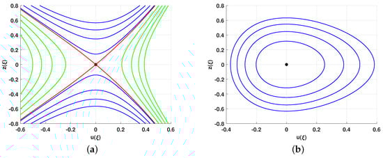
Figure 1.
Phase plane orbits for the system (6) if . Equilibria are shown by black solid circles; (a) ; (b) a = −1, −3.
Case II: If , then the two points and are equilibria for system (6), where . The eigenvalues (13) evaluated at the points O and are
Taking into account the existence condition for two equilibrium points, the two parameters a and c have the same sign, i.e., . Hence, they are either saddle and cusp if () as outlined by Figure 2a or center and cusp, respectively, as clarified by Figure 2b if ().
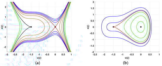
Figure 2.
Phase plane orbits for the system (6) if . The equilibria are indicated by the black solid circles; (a) , (b) a = −2, c = −2.
Case III: If , system (6) owns three equilibria. They are and . The eigenvalues (13) calculated at these points are
Based on the eigenvalues (15), we sum up the classification of the equilibria, O and , in Table 1 so as to avoid confusion.

Table 1.
Classification of the equilibria if .
Table 1.
Classification of the equilibria if .
| Case | Conditions | Nature | Figure | |||
|---|---|---|---|---|---|---|
| 1. | + | + | saddle | center | saddle | Figure 3a |
| 2. | − | − | center | center | saddle | Figure 3b |
| 3. | + | − | center | saddle | saddle | Figure 4a |
| 4. | − | + | saddle | center | center | Figure 4b |

Figure 3.
Phase portrait for the Hamiltonian system (6) in the phase plane () if and . The black solid circles are the equilibrium points; (a) ; (b) a = −1, c = −5/4.
Figure 3.
Phase portrait for the Hamiltonian system (6) in the phase plane () if and . The black solid circles are the equilibrium points; (a) ; (b) a = −1, c = −5/4.


Figure 4.
Phase plane orbits for the system (6) if and . The equilibria are indicated by the black solid circles; (a) ; (b) a = −1/15, .
Figure 4.
Phase plane orbits for the system (6) if and . The equilibria are indicated by the black solid circles; (a) ; (b) a = −1/15, .

The values of the parameter h at the equilibrium points are given by
3. Solutions
The aim of this section is to obtain some bounded wave solutions for Equation (1). These solutions are assorted into periodic, solitary, and kink (anti-kink) wave solutions. Besides, the same techniques can also be employed to construct unbounded wave solutions, but we avoid them because they are not physically meaningful. We now present the subsequent lemma, which will be substantial in the next analysis.
Lemma 1.
(see, e.g., [56,58,59]). Let system (6) has a continuous solution for and assume .
- (i)
- If , then the solution is solitary which corresponds to a homoclinic orbit for the system (6).
- (ii)
- If , then the solution is a kink (or anti-kink) wave that corresponds to a heteroclinic orbit for the system (6).
- (iii)
- If system (6) possesses a periodic orbit, then its corresponding solution is also periodic.
- (iv)
- If system (6) has a closed orbit in the phase portrait evolved by at least two centers and one separatrix layer, then its corresponding solution is a super periodic wave.
Based on the bifurcation theory and Lemma 1, we prove the next theorem.
Theorem 1.
Equation (1) does not possess any kink or anti-kink solutions.
Proof.
3.1. Periodic Solutions
We are interested in this subsection in deriving all periodic solutions of Equation (1). As we can see from the bifurcation analysis, Equation (1) has several periodic and super periodic solutions of different shapes. The following theorems enumerate these cases
Theorem 2.
Proof.
- (i)
- For fixed values of in the given range, system (6) owns different families of phase orbits. An orbit belonging to these families passes through the -axis twice which proves the existence of two real roots and two complex conjugate complex roots for . This enables us to write and consequently, the interval of real propagation is . Therefore, we assume . Integration of Equation (10) givesThe last equation gives the new periodic solutions (17) with a period of [60].
- (ii)
□
Theorem 3.
Proof.
For selecting values of in the given range, system (6) possesses a single orbit in red as illustrated by Figure 3b and it intersects -axis in and . Thus, reads as . The possible interval of real wave propagation . Assuming , the integration of (10) yields
which gives the solution as in the form (19). □
Theorem 4.
Proof.
For selecting values of in the given range, system (6) has two periodic families of orbits as outlined in Figure 3b and Figure 4b in green. An orbit belonging these families passes four times through -axis which indicates the existence of four real zeros for , i.e., . There are two possible intervals of real wave propagation. They are . We calculate the periodic wave solution along each interval individually.
□
Theorem 5.
Proof.
For selecting values of in the given range, system (6) has one periodic families of orbits as outlined in Figure 3a and Figure 4a in green. An orbit belonging these family intersects -axis in which indicates the existence of four real zeros for , i.e., . We calculate the periodic wave solution along with to give
which gives the new periodic solution as in the form (26) with a period of .
□
3.2. Solitary Solution
This subsection aims to construct solitary wave solutions for Equation (1) which correspond to the homoclinic orbits for the traveling wave system (6).
Theorem 6.
Proof.
For selecting values of in the given range, system (6) has homoclinic orbits in black as outlined as Figure 3b and Figure 4b, and an orbit of them cuts -axis in three points. Therefore, the polynomial has two simple roots and the other is double. reads as and the intervals of real wave propagation is . Integrate both sides of Equation (10) for and assuming and , respectively, we get the new solitary wave solutions (28) and (29). □
4. Graphical Representation
There are two goals for this section. The first is to graphically illustrate some of the solutions we have found, and the second is to investigate how altering one physical parameter while keeping the others constants, will affect the solution’s attitude. It is noted from Equation (3) that the variation in the parameters , and k have the same effect on the solutions, so we will only study one of them, say .
Let us assume and select a suitable initial condition implying to . System (6) has a periodic orbit around the center point as outlined by Figure 5a. Thus, the polynomial (11) has two real roots and two complex conjugate roots . Thanks to theorem 2, Equation (1) has a periodic solution in the form
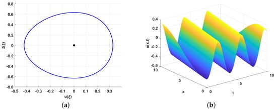
Figure 5.
Graphic representation for the periodic solution (30) and its corresponding orbit; (a) Periodic orbit; (b) 3D-periodic solution.
The 3D graphic representation of the solution (30) shows it is periodic as it is illustrated by Figure 5b.
The influence of varying the parameters on the periodic solutions is clarified in Figure 6, where the wave contracts as both its wavelength and its amplitude decrease with the increase of and as in Figure 6a,b, assuming the other parameters are fixed, while it expands with the increase of and w as in Figure 6c,d.
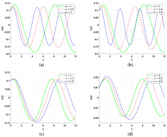
Figure 6.
The influence of parameters and w on the periodic solutions; (a) Influence of ; (b) Influence of ; (c) Influence of ; (d) Influence of w.
For the values , we select a suitable initial condition implying that satisfies . Consequently, system (6) has a super periodic orbit as outlined by Figure 7a. The polynomial in (11) has two real zeros which are also the intersection points of the orbit with -axis (see Figure 7a), i.e., , and the two conjugate complex roots . Following Theorem 2, Equation (1) has a super-periodic solution in the form
that is sketched in Figure 7b.
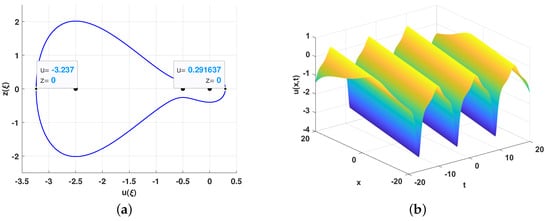
Figure 7.
Graphic representation for the super-periodic solution (31) and its corresponding orbit; (a) Super-periodic orbit; (b) 3D-super-periodic solution.
Remark 1.
Figure 8 illustrates the impacts of changing the parameters on the super periodic solutions. It is noted that the wave shrinks by increasing the values of each and as in Figure 8a,b, while it grows by increasing values of and w as in Figure 8c,d.
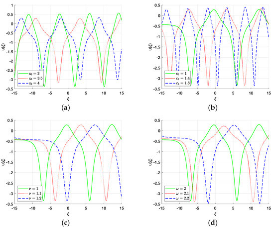
Figure 8.
The influence of parameters and w on the super-periodic solutions; (a) Influence of ; (b) Influence of ; (c) Influence of ; (d) Influence of w.
Assuming and selecting a suitable initial condition providing , system (6) has two homoclinic orbits each of them connecting the saddle point with it self as outlined by Figure 9a and it intersects -axis in the points and . Following [56], by virtue of Theorem 6, there are two types of solitary wave solutions in the form
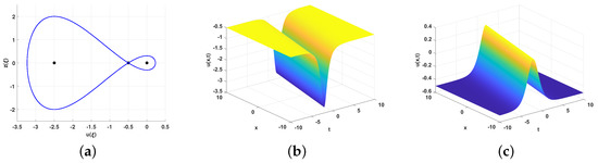
These solutions are named rarefactive wave solitary and compressive wave solitary, for more details about these solutions see, e.g., [56]. These solutions are clarified graphically by Figure 9. We examine graphically the influence of the included parameters on the the compressive soliton solution by introducing Figure 10. We find that both wavelength and the height decrease with the increase of as in Figure 10a, the wavelength decreases while the height remains constant with the increase of as in Figure 10b, the wavelength increases while the height remains constant with the increase of as in Figure 10c, and both wavelength and the height enlarge with the increase of w as in Figure 10d.
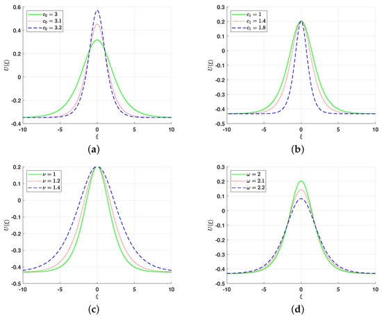
Figure 10.
The influence of parameters and w on compressive wave solitary solution; (a) Influence of ; (b) Influence of ; (c) Influence of ; (d) Influence of w.
5. Quasi Periodic Behaviour
In this section, we are concerned with a discussion of the autoresonance behavior for the non-autonomous system, i.e., the oscillator self-adjusts by subjecting the system to a variable periodic force. The perturbed form of problem (1) after inserting a periodic external force will be
Performing the transformation (2) to Equation (33), the corresponding perturbed dynamical system takes the form
where while and refer, respectively, to the strength and frequency of the external periodic force. We investigate the behavior of the perturbed system (34) for distinct values of by fixing both the remaining parameters and initial condition.
For fixed values , we select a suitable initial condition which implies the existence of a super periodic phase orbit outlined in Figure 3b in blue, for unperturbed system (6). The value of h corresponding to the initial condition is satisfying the condition . In the absence of the external periodic force, i.e., , the 2D and 3D phase portraits for the unperturbed system (6) are displayed in Figure 11a,d. To examine the behaviour for growing values of , we introduce the 2D and 3D phase portraits for perturbed system (34) for as outlined in Figure 11b,e and Figure 11c,f, respectively. We see that an increase in the strength of the external force reveals an increase in the periodic irregularity of the wave. It is noticeable the existence of a quasi-periodic behavior is due to the existence of two incommensurable frequencies in system (34).
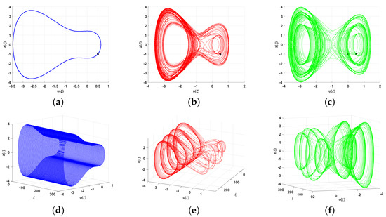
Figure 11.
2D and 3D phase portrait for the perturbed system (34) when and initial condition for fixed values of the parameters and various values of ; (a) ; (b) ; (c) ; (d) ; (e) ; (f) .
6. Discussion
This section aims to discuss the obtained results. We investigate the dynamical behavior for Equation (1) that is modeled for the elastic circular-rod wave-guide. It describes a double nonlinear wave equation with respect to the axial displacement gradient. As a consequence of the transverse Poisson effect, the longitudinal wave propagates simultaneously with the shear wave. Certain transformation involving wave variable (2) is applied to Equation (1) in order to convert it to second order differential equation that is followed by writing it as a dynamical system which is equivalent to the Hamilton system describing the one dimension motion of a particle. This equivalent has two significant roles in the current study. We summarize them in the next items:
- (a)
- It enables us to determine the interval of real wave propagation which corresponds to the interval of real motions in Hamilton systems.
- (b)
The integration of both sides of Equation (10) requires the range of the parameters . This range can be obtained by two distinct methods. They are bifurcation analysis and complete discriminate method of a polynomial . We apply the bifurcation analysis in this work for two reasons. They are
- (a)
- It gives us the required range of the parameters , and h. It also enables us to determine the type of the solution before constructing them via the type of the phase plane orbits as it is clarified in Lemma 1. By virtue of these facts, we prove the non-existence of kink or (anti-kink) wave solutions for Equation (1) as a result of system (6) has no heteroclinic phase orbit.
- (b)
- It manages us to clarify the dependence of the solutions on the initial conditions. The constant h in Equation (9) is determined from the initial conditions. Thus, for distinct values of h, or equivalently, for different initial conditions, there are different wave solutions. Let us illustrate this point by providing an example. If , then Equation (1) has either supper-periodic solution if , see theorem 2 or solitary solution if , see Theorem 6. Hence, for the same conditions on the physical parameters, the type of the solution depends on h which is always calculated from the initial conditions. Or, equivalently, the type of the solution depends on the initial conditions. Thus, we can also conclude that the bifurcation analysis enables us to find all possible wave solutions.
We illustrate graphically some of the obtained solutions by displaying the 3D-graphical representation and the corresponding phase orbit. Moreover, we investigate the influence of the included parameters , and on the solutions when one of them varies while the others are kept fixed. Figure 6, Figure 8 and Figure 10, clarify the influence of the parameters on periodic, supper-periodic and solitary solutions, respectively. These effects appear on both the amplitude and the width of the solutions.
Finally, we study the existence of quasi-behavior for the Hamilton system (6) after allowing a periodic perturbed term which is an external periodic force to act on the rod. After adding this term, system (6) which is named here as an unperturbed system is converted into perturbed system (34). For selected values of the parameters and suitable choice of the initial condition, the 2D and 3D phase portrait is outlined by Figure 11.
7. Conclusions
The study of some qualitative properties for the problem of a finite deformation flexible rod is really the focus of the present work. The governing equations, which are nonlinear partial differential equations, have been derived by applying Hamilton’s variational principle. The governing equation has been converted into one degree of freedom Hamiltonian system describing the one-dimensional motion of a particle utilizing specific wave transformation. In this context, the problem of finding wave solutions and the problem of establishing the solution of the Hamiltonian are equivalent. This equivalence is significant because it enables us to find the real wave solutions which have been limited by determining the interval of real wave propagation, which is also a permitted interval of particle real motions. In other words, it enables us to find bounded real-wave solutions that are desirable in real-world applications instead of complex solutions. Analyses of bifurcation and phase plane description have been carried out. This study has been utilized to prove the governing equation has no kink or anti-kink solutions and has solitary, periodic, and unbounded wave solutions. Based on the bifurcation constraints on the problem’s parameters, the conserved quantity has been integrated along the bounded phase plane orbits. Thus, we have discovered various periodic and solitary wave solutions that are displayed of them by exhibiting a 3D, contour, and the appropriate phase orbit. We have investigated how altering one physical parameter while preserving the other’s constant will affect the solutions we have found. Finally, We have examined numerically the phase plane after allowing periodic forces to act on the rod. We have concluded the perturbed system has a quasi-periodic behavior.
The investigation of chaotic behavior for system (34) and its applications to image encryption will be considered in our upcoming work.
Author Contributions
The authors contributed equally to this work. All authors have read and agreed to the published version of the manuscript.
Funding
The authors extend their appreciation to the Deanship of Scientific Research, Vice Presidency for Graduate Studies and Scientific Research, King Faisal University, Saudi Arabia for funding this research work through project number Grant No. 2257.
Institutional Review Board Statement
Not applicable.
Informed Consent Statement
Not applicable.
Data Availability Statement
Not applicable.
Acknowledgments
This work was supported through the Annual Funding track by the Deanship of Scientific Research, Vice Presidency for Graduate Studies and Scientific Research, King Faisal University, Saudi Arabia [Grant.2257].
Conflicts of Interest
The authors declare no conflict of interest.
References
- Arshad, M.; Seadawy, A.R.; Lu, D. Elliptic function and solitary wave solutions of the higher-order nonlinear Schrödinger dynamical equation with fourth-order dispersion and cubic-quintic nonlinearity and its stability. Eur. Phys. J. Plus 2017, 132, 371. [Google Scholar] [CrossRef]
- Arshad, M.; Seadawy, A.; Lu, D.; Wang, J. Travelling wave solutions of Drinfel’d–Sokolov–Wilson, Whitham–Broer–Kaup and (2 + 1)-dimensional Broer–Kaup–Kupershmit equations and their applications. Chin. J. Phys. 2017, 55, 780–797. [Google Scholar] [CrossRef]
- Seadawy, A.R.; Nuruddeen, R.; Aboodh, K.; Zakariya, Y. On the exponential solutions to three extracts from extended fifth-order KdV equation. J. King Saud Univ.-Sci. 2020, 32, 765–769. [Google Scholar] [CrossRef]
- Nasreen, N.; Seadawy, A.R.; Lu, D.; Arshad, M. Solitons and elliptic function solutions of higher-order dispersive and perturbed nonlinear Schrödinger equations with the power-law nonlinearities in non-Kerr medium. Eur. Phys. J. Plus 2019, 134, 485. [Google Scholar] [CrossRef]
- Younas, U.; Seadawy, A.R.; Younis, M.; Rizvi, S. Optical solitons and closed form solutions to the (3 + 1)-dimensional resonant Schrödinger dynamical wave equation. Int. J. Mod. Phys. B 2020, 34, 2050291. [Google Scholar] [CrossRef]
- Hossen, M.B.; Roshid, H.O.; Ali, M.Z. Multi-soliton, breathers, lumps and interaction solution to the (2 + 1)-dimensional asymmetric Nizhnik-Novikov-Veselov equation. Heliyon 2019, 5, e02548. [Google Scholar] [CrossRef]
- Manukure, S.; Chowdhury, A.; Zhou, Y. Complexiton solutions to the asymmetric Nizhnik–Novikov–Veselov equation. Int. J. Mod. Phys. B 2019, 33, 1950098. [Google Scholar] [CrossRef]
- Cattani, C.; Sulaiman, T.A.; Baskonus, H.M.; Bulut, H. On the soliton solutions to the Nizhnik-Novikov-Veselov and the Drinfel’d-Sokolov systems. Opt. Quantum Electron. 2018, 50, 138. [Google Scholar] [CrossRef]
- Li, Z. Diverse oscillating soliton structures for the (2 + 1)-dimensional Nizhnik–Novikov–Veselov equation. Eur. Phys. J. Plus 2020, 135, 8. [Google Scholar] [CrossRef]
- Iqbal, M.; Seadawy, A.R.; Khalil, O.H.; Lu, D. Propagation of long internal waves in density stratified ocean for the (2 + 1)-dimensional nonlinear Nizhnik-Novikov-Vesselov dynamical equation. Results Phys. 2020, 16, 102838. [Google Scholar] [CrossRef]
- Seadawy, A.R.; Arshad, M.; Lu, D. The weakly nonlinear wave propagation of the generalized third-order nonlinear Schrödinger equation and its applications. Waves Random Complex Media 2022, 32, 819–831. [Google Scholar] [CrossRef]
- Taghizadeh, N.; Mirzazadeh, M.; Farahrooz, F. Exact solutions of the nonlinear Schrödinger equation by the first integral method. J. Math. Anal. Appl. 2011, 374, 549–553. [Google Scholar] [CrossRef]
- ur Rehman, H.; Awan, A.U.; Habib, A.; Gamaoun, F.; El Din, E.M.T.; Galal, A.M. Solitary wave solutions for a strain wave equation in a microstructured solid. Results Phys. 2022, 39, 105755. [Google Scholar] [CrossRef]
- Rehman, H.U.; Iqbal, I.; Subhi Aiadi, S.; Mlaiki, N.; Saleem, M.S. Soliton solutions of Klein–Fock–Gordon equation using Sardar subequation method. Mathematics 2022, 10, 3377. [Google Scholar] [CrossRef]
- Asjad, M.I.; Inc, M.; Iqbal, I. Exact solutions for new coupled Konno–Oono equation via Sardar subequation method. Opt. Quantum Electron. 2022, 54, 798. [Google Scholar]
- Asjad, M.I.; Munawar, N.; Muhammad, T.; Hamoud, A.A.; Emadifar, H.; Hamasalh, F.K.; Azizi, H.; Khademi, M. Traveling wave solutions to the Boussinesq equation via Sardar sub-equation technique. AIMS Math. 2022, 7, 11134–11149. [Google Scholar]
- Rehman, H.U.; Awan, A.U.; Allahyani, S.A.; Tag-ElDin, E.M.; Binyamin, M.A.; Yasin, S. Exact solution of paraxial wave dynamical model with Kerr Media by using ϕ6 model expansion technique. Results Phys. 2022, 42, 105975. [Google Scholar] [CrossRef]
- El-Ganaini, S. Solitons and other solutions to a new coupled nonlinear Schrodinger type equation. J. Egypt. Math. Soc. 2017, 25, 19–27. [Google Scholar] [CrossRef]
- Seadawy, A.R.; Arshad, M.; Lu, D. Dispersive optical solitary wave solutions of strain wave equation in micro-structured solids and its applications. Phys. A Stat. Mech. Its Appl. 2020, 540, 123122. [Google Scholar] [CrossRef]
- Kumar, S.; Kumar, A.; Wazwaz, A.M. New exact solitary wave solutions of the strain wave equation in microstructured solids via the generalized exponential rational function method. Eur. Phys. J. Plus 2020, 135, 870. [Google Scholar] [CrossRef]
- Seadawy, A.R.; Ali, A.; Baleanu, D.; Althobaiti, S.; Alkafafy, M. Dispersive analytical wave solutions of the strain waves equation in microstructured solids and Lax’fifth-order dynamical systems. Phys. Scr. 2021, 96, 105203. [Google Scholar] [CrossRef]
- Jadaun, V.; Kumar, S. Lie symmetry analysis and invariant solutions of (3 + 1)(3 + 1)-dimensional Calogero–Bogoyavlenskii–Schiff equation. Nonlinear Dyn. 2018, 93, 349–360. [Google Scholar] [CrossRef]
- Tu, J.M.; Tian, S.F.; Xu, M.J.; Zhang, T.T. On Lie symmetries, optimal systems and explicit solutions to the Kudryashov–Sinelshchikov equation. Appl. Math. Comput. 2016, 275, 345–352. [Google Scholar] [CrossRef]
- El-Dessoky, M.; Elmandouh, A. Qualitative analysis and wave propagation for Konopelchenko-Dubrovsky equation. Alex. Eng. J. 2023, 67, 525–535. [Google Scholar] [CrossRef]
- Adeyemo, O.D.; Khalique, C.M.; Gasimov, Y.S.; Villecco, F. Variational and non-variational approaches with Lie algebra of a generalized (3 + 1)-dimensional nonlinear potential Yu-Toda-Sasa-Fukuyama equation in Engineering and Physics. Alex. Eng. J. 2023, 63, 17–43. [Google Scholar] [CrossRef]
- Wang, K. Exact travelling wave solution for the local fractional Camassa-Holm-Kadomtsev-Petviashvili equation. Alex. Eng. J. 2023, 63, 371–376. [Google Scholar] [CrossRef]
- Ahmed, M.S.; Zaghrout, A.A.; Ahmed, H.M. Travelling wave solutions for the doubly dispersive equation using improved modified extended tanh-function method. Alex. Eng. J. 2022, 61, 7987–7994. [Google Scholar] [CrossRef]
- Ali, K.K.; Osman, M.; Abdel-Aty, M. New optical solitary wave solutions of Fokas-Lenells equation in optical fiber via Sine-Gordon expansion method. Alex. Eng. J. 2020, 59, 1191–1196. [Google Scholar] [CrossRef]
- Rehman, H.U.; Awan, A.U.; Tag-ElDin, E.M.; Alhazmi, S.E.; Yassen, M.F.; Haider, R. Extended hyperbolic function method for the (2 + 1)-dimensional nonlinear soliton equation. Results Phys. 2022, 40, 105802. [Google Scholar] [CrossRef]
- Rehman, H.; Seadawy, A.R.; Younis, M.; Rizvi, S.; Anwar, I.; Baber, M.; Althobaiti, A. Weakly nonlinear electron-acoustic waves in the fluid ions propagated via a (3 + 1)-dimensional generalized Korteweg–de-Vries–Zakharov–Kuznetsov equation in plasma physics. Results Phys. 2022, 33, 105069. [Google Scholar] [CrossRef]
- Nemytskii, V.V. Qualitative Theory of Differential Equations; Princeton University Press: Princeton, NJ, USA, 2015; Volume 2083. [Google Scholar]
- Elbrolosy, M.; Elmandouh, A. Bifurcation and new traveling wave solutions for (2 + 1)-dimensional nonlinear Nizhnik–Novikov–Veselov dynamical equation. Eur. Phys. J. Plus 2020, 135, 533. [Google Scholar] [CrossRef]
- Elmandouh, A. Bifurcation and new traveling wave solutions for the 2D Ginzburg–Landau equation. Eur. Phys. J. Plus 2020, 135, 648. [Google Scholar] [CrossRef]
- Elmandouha, A.; Ibrahim, A. Bifurcation and travelling wave solutions for a (2 + 1)-dimensional KdV equation. J. Taibah Univ. Sci. 2020, 14, 139–147. [Google Scholar] [CrossRef]
- Al Nuwairan, M. The exact solutions of the conformable time fractional version of the generalized Pochhammer–Chree equation. Math. Sci. 2022, 1–12. [Google Scholar] [CrossRef]
- Karakoc, S.B.G.; Saha, A.; Sucu, D.Y. A collocation algorithm based on septic B-splines and bifurcation of traveling waves for Sawada–Kotera equation. Math. Comput. Simul. 2023, 203, 12–27. [Google Scholar] [CrossRef]
- Pradhan, B.; Saha, A. Coexistence of Chaotic, Quasiperiodic and Multiperiodic Features in Quantum Plasma. In Proceedings of the Seventh International Conference on Mathematics and Computing—ICMC, Online, 2–5 March 2021; pp. 903–914. [Google Scholar]
- Saha, A.; Pradhan, B.; Natiq, H. Multiperiodic and chaotic wave phenomena of collective ion dynamics under KP-type equation in a magnetised nonextensive plasma. Phys. Scr. 2022, 97, 095604. [Google Scholar] [CrossRef]
- Prasad, P.K.; Mandal, U.K.; Das, A.; Saha, A. Phase plane analysis and integrability via Bäcklund transformation of nucleus-acoustic waves in white dwarf. Chin. J. Phys. 2021, 73, 534–545. [Google Scholar] [CrossRef]
- Mohammed, W.W.; Al-Askar, F.M.; Cesarano, C.; Botmart, T.; El-Morshedy, M. Wiener process effects on the solutions of the fractional (2 + 1)-dimensional Heisenberg ferromagnetic spin chain equation. Mathematics 2022, 10, 2043. [Google Scholar] [CrossRef]
- Mohammed, W.W.; Al-Askar, F.M.; Cesarano, C.; El-Morshedy, M. The Optical Solutions of the Stochastic Fractional Kundu–Mukherjee–Naskar Model by Two Different Methods. Mathematics 2022, 10, 1465. [Google Scholar] [CrossRef]
- Mohammed, W.W.; Alshammari, M.; Cesarano, C.; Albadrani, S.; El-Morshedy, M. Brownian Motion Effects on the Stabilization of Stochastic Solutions to Fractional Diffusion Equations with Polynomials. Mathematics 2022, 10, 1458. [Google Scholar] [CrossRef]
- Elbrolosy, M.; Elmandouh, A. Dynamical behaviour of nondissipative double dispersive microstrain wave in the microstructured solids. Eur. Phys. J. Plus 2021, 136, 955. [Google Scholar] [CrossRef]
- Elmandouh, A. Integrability, qualitative analysis and the dynamics of wave solutions for Biswas–Milovic equation. Eur. Phys. J. Plus 2021, 136, 638. [Google Scholar] [CrossRef]
- Elbrolosy, M. Qualitative analysis and new soliton solutions for the coupled nonlinear Schrödinger type equations. Phys. Scr. 2021, 96, 125275. [Google Scholar] [CrossRef]
- Elbrolosy, M.; Elmandouh, A.; Elmandouh, A. Construction of new traveling wave solutions for the (2 + 1) dimensional extended Kadomtsev-Petviashvili equation. J. Appl. Anal. Comput. 2022, 12, 533–550. [Google Scholar] [CrossRef]
- Elmandouh, A.A.; Elbrolosy, M.E. New traveling wave solutions for Gilson–Pickering equation in plasma via bifurcation analysis and direct method. Math. Methods Appl. Sci. 2022. [Google Scholar] [CrossRef]
- Elbrolosy, M.; Elmandouh, A. Dynamical behaviour of conformable time-fractional coupled Konno-Oono equation in magnetic field. Math. Probl. Eng. 2022, 2022, 3157217. [Google Scholar] [CrossRef]
- Elmandouh, A.; Elbrolosy, M. Integrability, variational principal, bifurcation and new wave solutions for Ivancevic option pricing model. J. Math. 2022, 2, 3. [Google Scholar]
- Liu, Z.F.; Zhang, S.Y. Solitary waves in finite deformation elastic circular rod. Appl. Math. Mech. 2006, 27, 1255–1260. [Google Scholar] [CrossRef]
- Liu, S.K.; Liu, S. Nonlinear Equations in Physics; Peking University Press: Beijing, China, 2000. [Google Scholar]
- Porubov, A.V.; Velarde, M.G. On nonlinear waves in an elastic solid. Comptes Rendus Acad. Sci.-Ser. IIB-Mech. 2000, 328, 165–170. [Google Scholar] [CrossRef]
- Zhang, S.; Guo, J.; Zhang, N. The dynamics behaviors and wave properties of finite deformation elastic rods with viscous or geometrical-dispersive effects. In Proceedings of the Forth International Conference on Nonlinear Mechanics—ICNM-IV, Shanghai, China, 14–17 August 2002; pp. 728–732. [Google Scholar]
- Fu, Z.; Liu, S.; Liu, S. New transformations and new approach to find exact solutions to nonlinear equations. Phys. Lett. A 2002, 299, 507–512. [Google Scholar] [CrossRef]
- Goldstein, H. Classical Mechanics; Addison-Wesley Series in Physics; Addison-Wesley: Boston, MA, USA, 1980. [Google Scholar]
- Saha, A.; Banerjee, S. Dynamical Systems and Nonlinear Waves in Plasmas; CRC Press: Boca Raton, FL, USA, 2021; pp. x+207. [Google Scholar]
- Yang, L.; Hou, X.; Zeng, Z. A complete discrimination system for polynomials. Sci. China Ser. E 1996, 39, 628–646. [Google Scholar]
- Meng, Q.; He, B.; Long, Y.; Rui, W. Bifurcations of travelling wave solutions for a general Sine–Gordon equation. Chaos Solitons Fractals 2006, 29, 483–489. [Google Scholar] [CrossRef]
- Bin, H.; Jibin, L.; Yao, L.; Weiguo, R. Bifurcations of travelling wave solutions for a variant of Camassa–Holm equation. Nonlinear Anal. Real World Appl. 2008, 9, 222–232. [Google Scholar] [CrossRef]
- Byrd, P.F.; Friedman, M.D. Handbook of Elliptic Integrals for Engineers and Scientists, 2nd ed., revised; Die Grundlehren der Mathematischen Wissenschaften, Band 67; Springer: New York, NY, USA; Berlin/Heidelberg, Germany, 1971; pp. xvi+358. [Google Scholar]


Disclaimer/Publisher’s Note: The statements, opinions and data contained in all publications are solely those of the individual author(s) and contributor(s) and not of MDPI and/or the editor(s). MDPI and/or the editor(s) disclaim responsibility for any injury to people or property resulting from any ideas, methods, instructions or products referred to in the content. |
© 2023 by the authors. Licensee MDPI, Basel, Switzerland. This article is an open access article distributed under the terms and conditions of the Creative Commons Attribution (CC BY) license (https://creativecommons.org/licenses/by/4.0/).