

A Gain Scheduling Design Method of the Aero-Engine Fuel Servo Constant Pressure Valve with High Accuracy and Fast Response Ability

Abstract
:1. Introduction
- Firstly, the design theory of the system is revealed successfully by using the linear incremental analysis method. Evidently, the controlled object and the stabilization controller are the two fundamental units of the closed-loop system, as demonstrated by the study results.
- Secondly, the accurate loop transfer function models of the system are calculated. In addition, the precise influences of the design parameters on the dynamic performance and stability are analyzed by using the bode frequency domain analysis methods, and some useful guidance measures are offered.
- Finally, a gain scheduling design method for the stabilization control gain is proposed, and the proposed method is demonstrated to exactly solve the design work based on the nonlinear simulation.
2. Design Analysis and Dynamic Equations
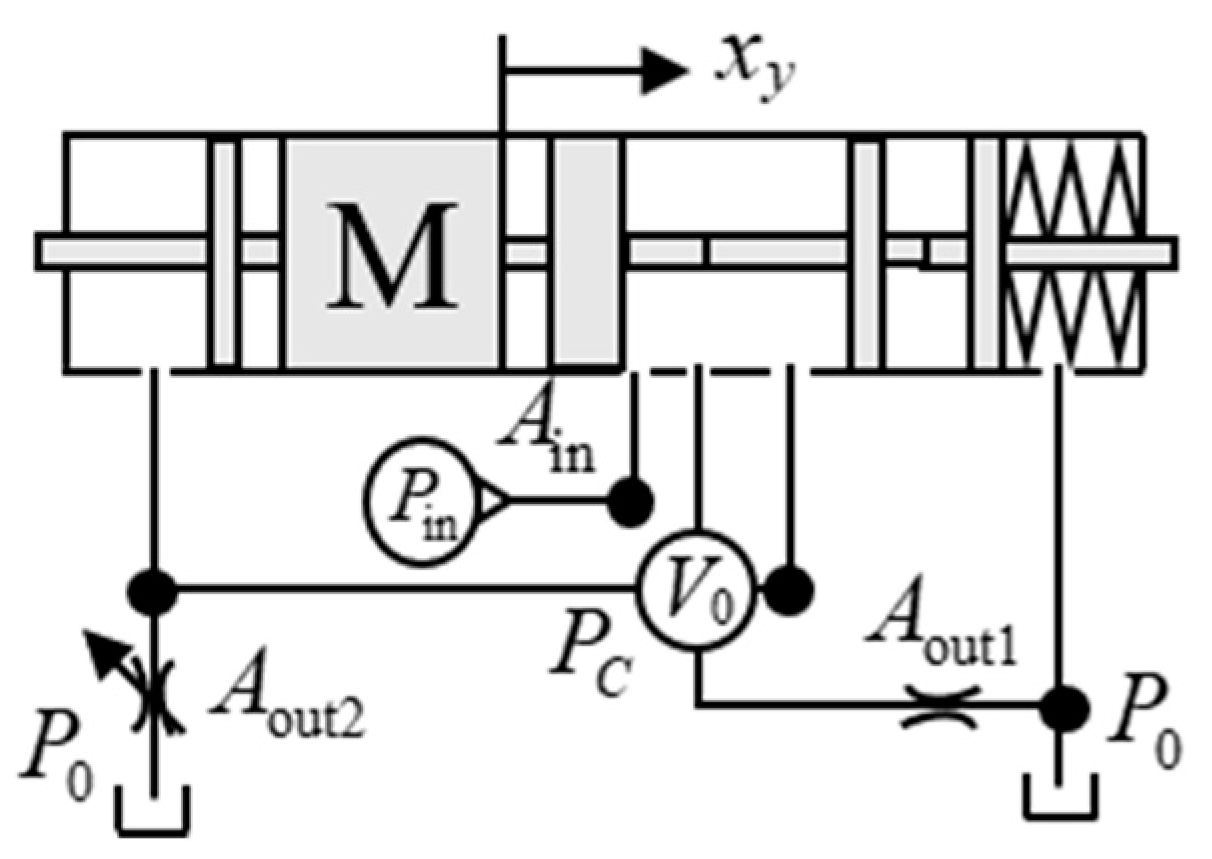
2.1. Design Analysis
- is the dynamic matrix of the controlled object.
- is the dynamic matrix of the motion valve, is the generalized stabilization control gain, and they construct the stabilization controller.
2.2. Dynamic Equations
2.2.1. Controlled Object
2.2.2. Stabilization Controller
3. Linear Models
3.1. Open-Loop Transfer Function
3.2. Disturbance Input Transfer Functions
3.3. Control Output Transfer Functions
- The closed-loop disturbance transfer function from to is
- 2.
- The closed-loop disturbance transfer function from to is
4. Bode Frequency Domain Characteristic Analysis
4.1. Calculation of the Corner Frequencies
- If , the second-order section is an underdamped oscillation link, and its poles are
- 2.
- If , the second-order section is an overdamped non-oscillation link, and its poles are
- The stabilization control gain mainly influences and the open-loop gain ;
- The spring stiffness mainly influences , , and the open-loop gain ;
- The volume of the controlled chamber mainly influences ;
- The pressure-bearing area mainly influences and the open-loop gain ;
- The mass mainly influences and .
4.2. Analysis of the Frequency Domain Characteristic
- Reducing the stabilization control gain ;
- Reducing the mass of the motion valve ;
- Increasing the viscous friction coefficient .
- Increasing the stabilization control gain ;
- Reducing the spring stiffness ;
- Reducing the pressure-bearing area of the motion valve.
4.3. Influence of the Stabilization Control Gain on the Frequency Domain Characteristic
- According to Equations (20) and (22), the steady-state gain and decrease, thus the steady error caused by the disturbance inputs is reduced, resulting in better disturbance rejection performance;
- The crossover frequency increases and the regulating time is reduced, resulting in faster response performance;
- The phase margin decreases, resulting in worse robustness performance.
4.4. Stability Analysis
5. Gain Scheduling Design Method
- Steady-state performance: The designed controlled pressure is , and the working range is .
- Dynamic performance: The regulation time is not greater than .
5.1. Dynamic Design
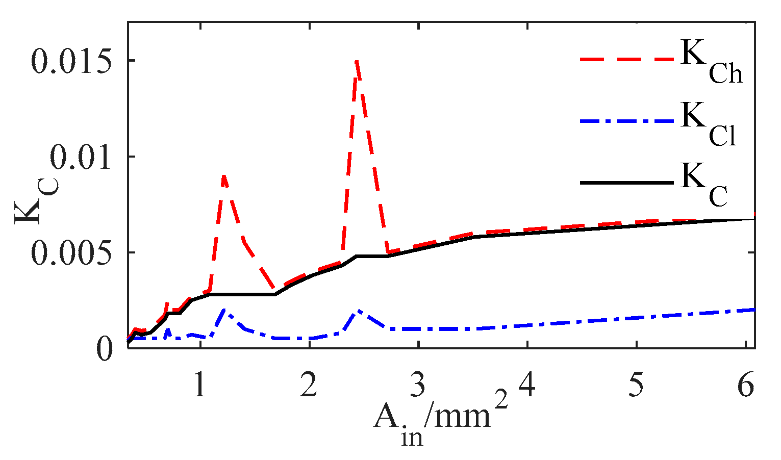
5.1.1. Calculation of the Stabilization Control Gain
5.1.2. Constraint Condition
5.2. Calculation processes
6. Design and Simulation
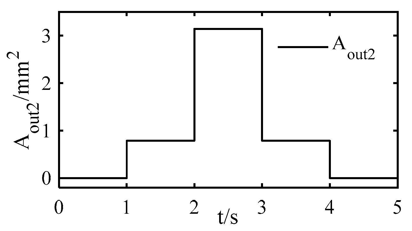
- The working range of the variable outlet flow area is [0, 3.1416] × 10−6 m2.
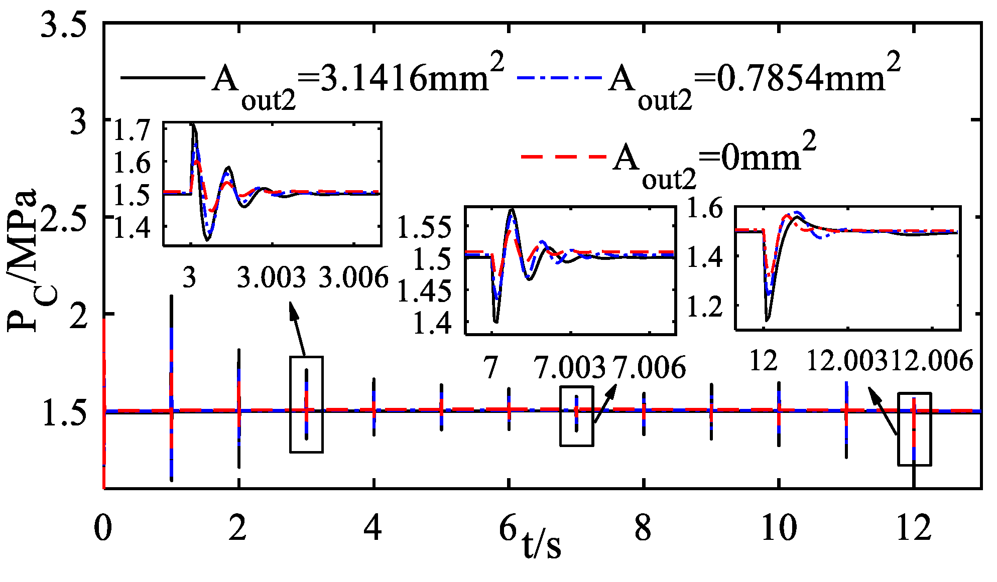
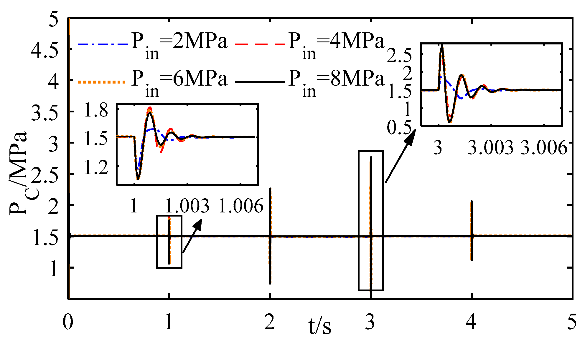
- The designed controlled pressure is 1.5 ± 0.01 MPa;
- The designed regulating time is not more than 0.006 s.
- Designing the stabilization control law as .
6.1. Design
- Since the designed pressure is 1.5 MPa, according to Equation (43), the steady-state spring compression is 13.404129 mm;
- Since the design range of is [1.49, 1.51] MPa, according to Equation (44), the variation of the spring compression is 0.22340214 mm.
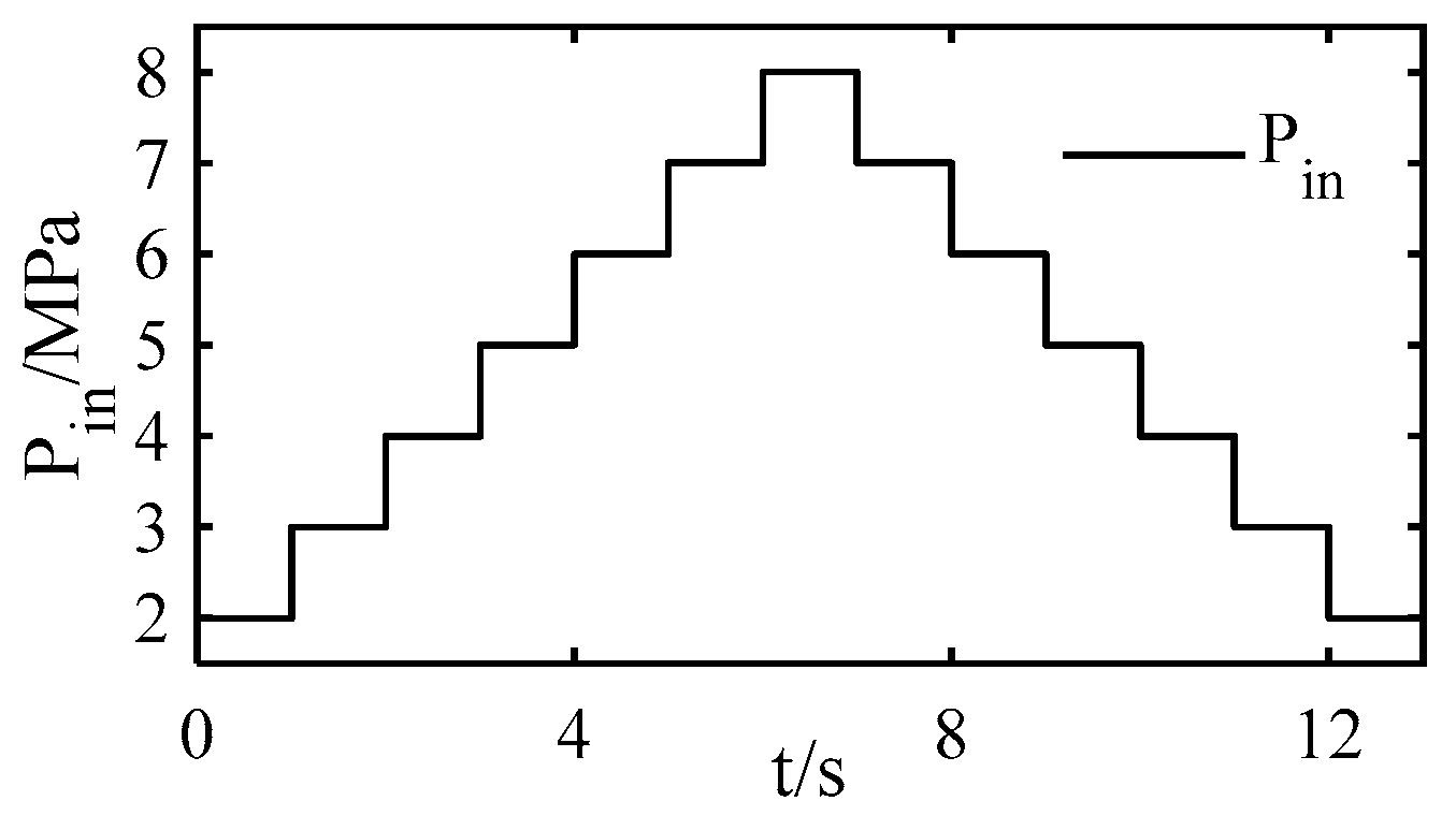
6.2. Simulation
7. Conclusions
- The linear incremental analysis method vividly displays the design theory of the constant pressure valve when compared to the conventional direct transfer function transformation analysis method. In addition, the key design parameter, the stabilization control gain, is clarified, as well as the system’s input-output characteristics, which were not covered in earlier studies.
- The analysis results of the bode frequency domain characteristics explain quantitatively how the design parameters affect the system performance and give correct guidance to design the performance parameters, preventing trial and error in the research process.
- Evidently, when using the gain scheduling design method, both the steady-state and dynamic performance of the designed system satisfies the design requirements. The predesign and analysis of other components of the fuel metering system, including the position control system, can be realized using the proposed design methods.
Author Contributions
Funding
Data Availability Statement
Conflicts of Interest
References
- Wang, X.; Yang, S.B.; Zhu, M.Y.; Kong, X.X. Aeroengine Control Principles; Science Press: Beijing, China, 2021; pp. 59–106. [Google Scholar]
- Fan, S.Q.; Li, H.C.; Fan, D. Aeroengine control: Volume II; Northwest Polytechnic University Press: Xi’an, China, 2008; pp. 186–294. [Google Scholar]
- McCloy, D.; Martin, H.R. Control of Fluid Power, 2nd ed.; Ellis Horwood Limited: New York, NY, USA, 1980; pp. 1–150. [Google Scholar]
- Xu, C.S.; Jia, S.F.; Li, G. Analysis of the thrust pulsation of the aeroengine. Aviat. Maint. Eng. 2002, 222–224. [Google Scholar]
- Wang, H.W.; Wang, X.; Li, Z.P.; Dang, W. Quantitative analysis on constant pressure valve stability. J. Aerosp. Power 2015, 30, 754–761. [Google Scholar] [CrossRef]
- Liu, Q.H.; Jia, M.X. Study on linear and nonlinear characteristics of pilot pressure relief valve (Part 1). Modul. Mach. Tool Autom. Manuf. Tech. 1985, 19–23. Available online: http://www.cnki.com.cn/Article/CJFDTotal-ZHJC198509002.htm (accessed on 28 September 1985).
- Liu, Q.H.; Jia, M.X. Study on linear and nonlinear characteristics of pilot pressure relief valve (Part 2). Modul. Mach. Tool Autom. Manuf. Tech. 1985, 17–29. Available online: http://www.cnki.com.cn/Article/CJFDTOTAL-ZHJC198510003.htm (accessed on 28 October 1985).
- Zeng, X.R.; Song, T.T. Steady state hydraulic compensation single stage overflow valve and its experimental study. Mach. Tool Hydraul. 1984, 12–19. Available online: http://www.cnki.com.cn/Article/CJFDTotal-JCYY198406001.htm (accessed on 26 December 1984).
- Li, S.N.; Ge, S.H. Development and research of new single stage overflow valve. Mach. Tool Hydraul. 1987, 24–32. Available online: http://www.cnki.com.cn/Article/CJFDTotal-JCYY198704004.htm (accessed on 29 August 1987).
- Ray, A. Dynamic modeling and simulation of a relief valve. Simulation 1978, 31, 167–172. [Google Scholar] [CrossRef]
- Yu, X.; Chen, H.H.; Zheng, Y.; Shi, H.Y. Modeling and simulation analysis of pressure relief valve based on AMESim. Hoisting Conveying Mach. 2011, 32–35. [Google Scholar] [CrossRef]
- Li, X.J.; Pan, Y.T.; Yue, X.K.; Ma, L.Q.; Lin, Y. Simulated analysis on the dynamic behavior influence caused by pilot valve parameters upon pilot operated pressure reducing valve. J. Taiyuan Univ. Technol. 2013, 44, 594–597, 603. [Google Scholar] [CrossRef]
- Hu, C.X. Dynamic modeling and simulation for converse unloading pressure reducing valve. Rocket. Propuls. 2014, 40, 60–64. [Google Scholar] [CrossRef]
- Wu, R.; Tang, W.; Lin, W.X. Dynamic performance simulation of pressure relief valve and test. J. Xiamen Univ. 2011, 50, 847–851. [Google Scholar]
- Zhang, L.; Li, W.F.; Zhao, Y.B.; Chao, C.H. Modeling and simulation of uniform-pressure-drop valve based on AMESim. Mech. Eng. Autom. 2013, 58–60. [Google Scholar] [CrossRef]
- Dong, J.W.; Ma, W.Q.; Guan, G.F. Simulation and dynamic characteristics analysis of a pressure reducing valve based on AMESim. Hydraul. Pneum. Seals 2015, 35, 46–49. [Google Scholar] [CrossRef]
- Gu, C.H.; Mao, H.P.; Wang, Q.; Shi, Y.C. Simulation analysis of direct-acting pressure reducing valves dynamic characteristics based on the AMESim. Mach. Des. Manuf. 2017, 234–237. [Google Scholar] [CrossRef]
- Zhou, F.; Gu, L.Y.; Chen, Z.H. Model linearization and stability analysis of thruster system controlled by proportional pressure reducing valves. J. Mech. Eng. 2017, 53, 187–194. [Google Scholar] [CrossRef]
- Teng, H.; Shi, Y.P.; Zhang, L.; Zang, H. Simulative and experimental study of dynamic characteristics of pressure relief valve based on AMESim. Aerospace 2015, 32, 48–53, 67. [Google Scholar] [CrossRef]
- Dasgupta, K.; Karmakar, R. Modelling and dynamics of single-stage pressure relief valve with directional damping. Simul. Model. Pract. Theory 2002, 10, 51–67. [Google Scholar] [CrossRef]
- Gabor, L.; Alan, C.; Csaba, H. Nonlinear analysis of a single stage pressure relief valve. IAENG Int. J. Appl. Math. 2009, 39. [Google Scholar] [CrossRef]
- Jiang, W.L.; Zhu, Y.; Yang, C. Study on nonlinear dynamic behavior of a hydraulic relief valve. China Mech. Eng. 2013, 24, 2705–2709. [Google Scholar] [CrossRef]
- He, X.F.; Zhao, D.X.; Sun, X.; Zhu, B.H. Theoretical and experimental research on a three-way water hydraulic pressure reducing valve. J. Press. Vessel. Technol. 2017, 139, 041601. [Google Scholar] [CrossRef]
- Shi, R.; Wang, C.; He, T.; Xie, T. Analysis of dynamic characteristics of pressure-regulating and pressure-limiting combined relief valve. Math. Probl. Eng. 2021, 1–13. [Google Scholar] [CrossRef]
- Merritt, H.E. Hydraulic Control System; John Wiley: New York, NY, USA, 1976. [Google Scholar]
- Sullivan, J.A. Fluid Power: Theory and Application, 4th ed.; Prentice-Hall: Hoboken, NJ, USA, 1998. [Google Scholar]
- Manring, N.D. Hydraulic Control System; John Wiley and Sons: New York, NY, USA, 2005. [Google Scholar]
- Zhang, Y. Hydraulic and Pneumatic Transmission; Electronic Industry Press: Beijing, China, 2011; pp. 113–114. [Google Scholar]


| Parameter/Unit | Value | Parameter/Unit | Value |
|---|---|---|---|
| /Kg | 0.0115 | /m3 | 10−5 |
| /(N·m/s) | 10 | /(Kg/m3) | 800 |
| /m | 0.008 | /bar | 17,000 |
| /MPa | 1.5 | /m | 0.001 |
| /MPa | 0.3 | 0.7 |
| /MPa | /mm | /mm2 | |||
|---|---|---|---|---|---|
| 2 | 2 | 6.08366800 | 0.139094570 | [0.002, 0.007] | 0.0068 |
| 1 | 2.43346720 | 0.041787194 | [0.002, 0.015] | 0.0048 | |
| 0 | 1.21673360 | 0.019299005 | [0.002, 0.009] | 0.0028 | |
| 3 | 2 | 3.51240740 | 0.034057185 | [0.001, 0.006] | 0.0058 |
| 1 | 1.40496290 | 0.011826533 | [0.001, 0.0055] | 0.0028 | |
| 0 | 0.70248147 | 0.006026016 | [0.001, 0.0025] | 0.0018 | |
| 4 | 2 | 2.72069900 | 0.020693472 | [0.0010, 0.005] | 0.0048 |
| 1 | 1.08827960 | 0.007491835 | [0.0005, 0.003] | 0.0028 | |
| 0 | 0.54413981 | 0.003934234 | [0.0005, 0.001] | 0.0008 | |
| 5 | 2 | 2.29941040 | 0.015556697 | [0.0008, 0.0045] | 0.0043 |
| 1 | 0.91976415 | 0.005747635 | [0.0007, 0.0027] | 0.0025 | |
| 0 | 0.45988207 | 0.003064452 | [0.0005, 0.0009] | 0.0007 | |
| 6 | 2 | 2.02788930 | 0.012802030 | [0.0005, 0.004] | 0.0038 |
| 1 | 0.81115574 | 0.004787408 | [0.0005, 0.002] | 0.0018 | |
| 0 | 0.40557787 | 0.002576085 | [0.0005, 0.001] | 0.0008 | |
| 7 | 2 | 1.83429490 | 0.011061443 | [0.0005, 0.0035] | 0.0033 |
| 1 | 0.73371797 | 0.004169889 | [0.0005, 0.0020] | 0.0018 | |
| 0 | 0.36685898 | 0.002257730 | [0.00055, 0.00065] | 0.0004 | |
| 8 | 2 | 1.68730590 | 0.009849004 | [0.0005, 0.0030] | 0.0028 |
| 1 | 0.67492237 | 0.003734197 | [0.0005, 0.0017] | 0.0015 | |
| 0 | 0.33746118 | 0.002030850 | [0.0004, 0.0005] | 0.0003 |
| mm2 | mm | |
|---|---|---|
| 0.33746118 | 0.0003 | 0 |
| 0.36685898 | 0.0004 | 0.097992667 |
| 0.40557787 | 0.0008 | 0.19478989 |
| 0.45988207 | 0.0007 | 0.26267014 |
| 0.54413981 | 0.0008 | 0.38303834 |
| 0.67492237 | 0.0015 | 0.54651654 |
| 0.70248147 | 0.0018 | 0.56488927 |
| 0.73371797 | 0.0018 | 0.58224289 |
| 0.81115574 | 0.0018 | 0.62526387 |
| 0.91976415 | 0.0025 | 0.68560187 |
| 1.0882796 | 0.0028 | 0.75300805 |
| 1.2167336 | 0.0028 | 0.79888448 |
| 1.4049629 | 0.0028 | 0.86610923 |
| 1.6873059 | 0.0028 | 0.96694602 |
| 1.8342949 | 0.0033 | 1.01944210 |
| 2.0278893 | 0.0038 | 1.07810710 |
| 2.2994104 | 0.0043 | 1.14956000 |
| 2.4334672 | 0.0048 | 1.18073600 |
| 2.7206990 | 0.0048 | 1.24057590 |
| 3.5124074 | 0.0058 | 1.40551520 |
| 6.0836680 | 0.0068 | 1.84883600 |
| mm2 | mm | |
|---|---|---|
| 0.33746118 | 0.0006 | 0 |
| 0.36685898 | 0.0007 | 0.045227385 |
| 0.40557787 | 0.0008 | 0.096852571 |
| 0.45988207 | 0.0008 | 0.16473282 |
| 0.54413981 | 0.0015 | 0.23800042 |
| 0.67492237 | 0.0017 | 0.31973952 |
| 0.70248147 | 0.0027 | 0.33226638 |
| 0.73371797 | 0.0018 | 0.34614927 |
| 0.81115574 | 0.0025 | 0.38216684 |
| 0.91976415 | 0.0027 | 0.42393931 |
| 1.0882796 | 0.0039 | 0.47500459 |
| 1.2167336 | 0.0100 | 0.49348718 |
| 1.4049629 | 0.0049 | 0.51875286 |
| 1.6873059 | 0.0040 | 0.58220073 |
| 1.8342949 | 0.0038 | 0.61989021 |
| 2.0278893 | 0.0055 | 0.66152342 |
| 2.2994104 | 0.0049 | 0.71373902 |
| 2.4334672 | 0.0160 | 0.72656742 |
| 2.7206990 | 0.0080 | 0.75050340 |
| 3.5124074 | 0.0075 | 0.85265932 |
| 6.0836680 | 0.0060 | 1.23358680 |
| mm | mm2 |
|---|---|
| 0 | 0 |
| 0.2 | 0.33746118 |
| 0.24522738 | 0.36685898 |
| 0.29685257 | 0.40557787 |
| 0.36473282 | 0.45988207 |
| 0.43800042 | 0.54413981 |
| 0.51973952 | 0.67492237 |
| 0.53226638 | 0.70248147 |
| 0.54614927 | 0.73371797 |
| 0.58216684 | 0.81115574 |
| 0.62393931 | 0.91976415 |
| 0.67500459 | 1.0882796 |
| 0.69348718 | 1.2167336 |
| 0.71875286 | 1.4049629 |
| 0.78220073 | 1.6873059 |
| 0.81989021 | 1.8342949 |
| 0.86152342 | 2.0278893 |
| 0.91373902 | 2.2994104 |
| 0.92656742 | 2.4334672 |
| 0.95050340 | 2.7206990 |
| 1.05265930 | 3.5124074 |
Disclaimer/Publisher’s Note: The statements, opinions and data contained in all publications are solely those of the individual author(s) and contributor(s) and not of MDPI and/or the editor(s). MDPI and/or the editor(s) disclaim responsibility for any injury to people or property resulting from any ideas, methods, instructions or products referred to in the content. |
© 2022 by the authors. Licensee MDPI, Basel, Switzerland. This article is an open access article distributed under the terms and conditions of the Creative Commons Attribution (CC BY) license (https://creativecommons.org/licenses/by/4.0/).
Share and Cite
Zhao, W.; Wang, X.; Jiang, Z.; Long, Y. A Gain Scheduling Design Method of the Aero-Engine Fuel Servo Constant Pressure Valve with High Accuracy and Fast Response Ability. Symmetry 2023, 15, 45. https://doi.org/10.3390/sym15010045
Zhao W, Wang X, Jiang Z, Long Y. A Gain Scheduling Design Method of the Aero-Engine Fuel Servo Constant Pressure Valve with High Accuracy and Fast Response Ability. Symmetry. 2023; 15(1):45. https://doi.org/10.3390/sym15010045
Chicago/Turabian StyleZhao, Wenshuai, Xi Wang, Zhen Jiang, and Yifu Long. 2023. "A Gain Scheduling Design Method of the Aero-Engine Fuel Servo Constant Pressure Valve with High Accuracy and Fast Response Ability" Symmetry 15, no. 1: 45. https://doi.org/10.3390/sym15010045
APA StyleZhao, W., Wang, X., Jiang, Z., & Long, Y. (2023). A Gain Scheduling Design Method of the Aero-Engine Fuel Servo Constant Pressure Valve with High Accuracy and Fast Response Ability. Symmetry, 15(1), 45. https://doi.org/10.3390/sym15010045