Abstract
In this study, we establish a novel Lorentzian interpretation of the Euler–Savary () and Disteli () formulae. Subsequently, we proceed to establish a theoretical structure for a Lorentzian torsion line congruence which is the spatial symmetry of the Lorentzian circling-point dual curve, in accordance with the principles of the kinematic theory of spherical locomotions. Further, a timelike () torsion line congruence is defined and its spatial equivalence is examined. The findings contribute to an enhanced comprehension of the interplay between axodes and Lorentzian spatial movements, which has possible significance in various disciplines, such as the fields of robotics and mechanical engineering.
MSC:
53A15; 53A17; 53A25; 53A35
1. Introduction
The concept of the instantaneous screw axis () of a moving body is well-established. This axis gives rise to two distinct ruled surfaces, known as the mobile and immobile axodes, with as their creating line in the movable space and in the steady space, respectively. The axodes exhibit both sliding and rolling motion relative to each other along a defined trajectory, which ensures that the tangential contact between the axodes remains constant throughout the entire length of the two matting rulings (one being in all axodes), which simultaneously motivate the at any instant. at any given moment. It is appreciable that not only does a certain suitable locomotion lead to a unique set of axodes but the opposite also occurs. This designates that, should the axodes of any locomotion be recognized, the private locomotion can be recreated without awareness of the physical constituents of the mechanism, their organization, distinct dimensions, or the designates by which they are attached [1,2,3,4,5]. The recruitment of axodes in the execution of composition is enhanced as manifest by examination showing that the axodes are central within the physical mechanism and the actual locomotion of its constituents. For instance: Garnier [6] was the first to address the issue of the kinematics ownership of the instantaneous locomotion created by the axodes up to the second order. Then, he gave the formulae for the spherical locomotion by appointing the spherical polodes. A procedure for appointing and finding its characteristics was advanced by Phillips and Hunt [7]. Skreiner [8] assigned the intermediate modification of the by the intermediary of a spatial locomotion and researched numerous distinct cases. Diziogly [9] suggested that the action be utilized to determine the -axis, taking into consideration the local characteristics of the axodes. Abdel-Baky and Al-Solamy [10] proposed a novel geometric-kinematic approach to one-parameter locomotion based on facts describing the locomotion of the axodes. A significant amount of research exists concerning the and the axode invariants [11,12,13,14,15,16,17,18,19].
The discovery of dual numbers is attributed to W. Clifford, who was the first to identify their existence. Subsequently, E. Study employed dual numbers as a tool to investigate the properties of locomotions and line geometry. The theorist attracted attention to the performance of straight lines through the utilization of dual unit vectors. Additionally, he identified and established the mapping that is commonly associated with his name, known as the E. Study map. The collection of all oriented lines in Euclidean 3-space is in bijection with a set of points on the dual unit sphere () in the dual 3-space . Further characteristics of the E. Study map and screw calculus can be found in [8,9,20,21,22]. By utilizing these works, if we adopt the Minkowski 3-space as an alternative of , the situation frequently has more features than the Euclidean case. In , the distance can be positive, negative or zero, while the distance in is strictly limited to positive values. Thus, it is necessary to differentiate oriented lines based on the value of distance determining whether it is positive, negative, or zero. Oriented lines with ( are named timelike () (spacelike ()) oriented lines and oriented lines with are named null lines [23,24,25,26].
In this paper, the invariants of the axodes are utilized for extracting new Lorentzian proofs of the and formulae. Symmetrical to the kinematic theory of spherical movement, the well known cubic of the steady curvature is discovered on a Lorentzian dual unit sphere. Afterward, a torsion line congruence is elucidated and its spatial synonym is scrutinized. The advanced statements degenerate into a quadratic form, which can readily enable evident understanding into the geometric estates of the torsion line congruence.
2. Preliminaries
An outline of dual numbers theory and the dual Lorentzian vectors is specified in [23,24,25,26,27,28]. If and are real numbers, then a dual number can be designed as: , such that and . This is, in fact, quite analogous to the notion of a complex number, the prime singularity being in a complex number . Then, the set
shared with the Lorentzian metric
is a dual Lorentzian 3-space . A dual vector is a dual if or , a dual if , and a lightlike () or null dual if and . If , the norm of is
then, the vector is a () dual unit vector if (). It is uncomplicated that
The 6-components and of and are the normed Plücker coordinates. For any two dual vectors and of , the vector product is
where , , is the canonical dual basis of . The hyperbolic and Lorentzian (de Sitter space) dual unit () spheres, respectively, are
and
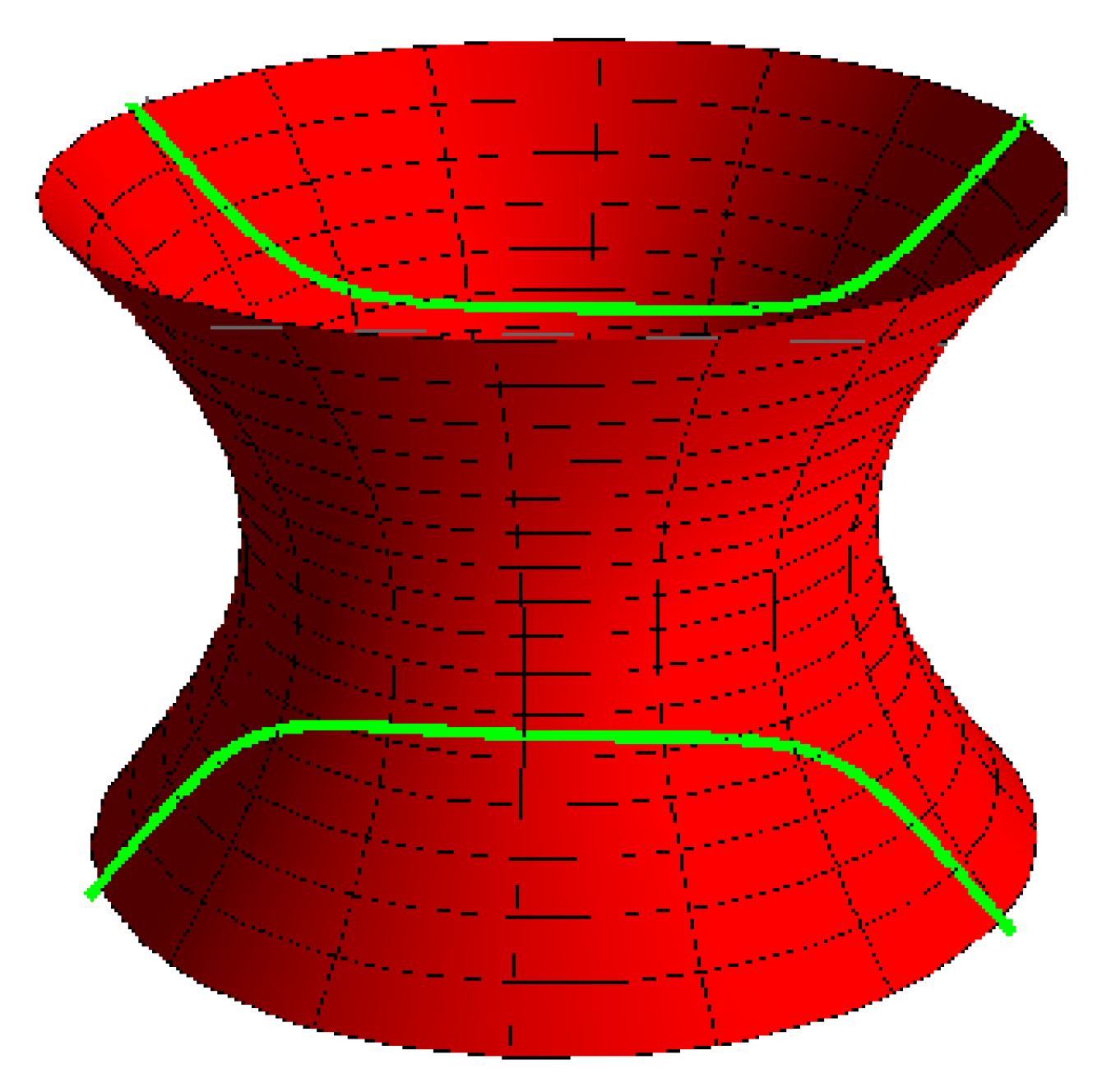
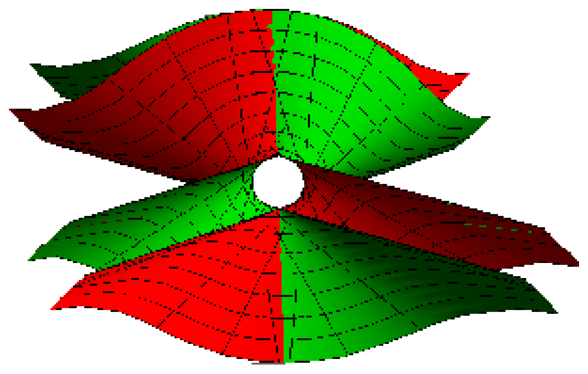
Through this, we are presented with the map provided by E. Study. The spheres are formulated as a couple of integrate hyperboloids. The shared asymptotic cone illustrates the set of null lines, the ring constituted hyperboloid illustrates the set of lines, and the oval constituted hyperboloid illustrates the set of lines The reverse points of each hyperboloid illustrate the couple of reverse vectors on a non-null line (see Figure 1).

Figure 1.
The dual hyperbolic and dual Lorentzian unit spheres.
Via the E. Study map, a smooth curve is a ruled surface in Minkowski 3-space . Correspondingly, a smooth curve is a or ruled surface in . are distinguished by their rulings, and we no longer differentiate between a ruled surface and its dual curve image.
Lorentzian Dual Spherical Locomotion
Let us assume that and are two Lorentzian spheres centered at the origin in . Let the orthonormal dual frames ;()} and ;(),,} be rigidly linked to and , respectively. We set that is fixed, whereas the components of the set are functions of a real parameter . Then, we contemplate that is movable with respect to The explication of this is as follows: the rigidly correlated with movable over the is rigidly correlated with . This locomotion is a one-parameter dual spherical locomotion and is represented by . If and correlate with the Lorentzian line spaces and , respectively, then correlate with the one-parameter Lorentzian spatial locomotion Therefore, is the movable Lorentzian space with respect to the unmovable Lorentzian space [23,24,25,26,27,28].
We will now locate the auxiliary dual frame by the first order instantaneous assets of the locomotion. We locate gg as the , gg, and . The set so specified will be an auxiliary Blaschke frame. Hence, via the E. Study map, one can generate two ruled surfaces: one is in -space and the other is in -space. The first ruled surface is called the steady axode , whereas the second is called the movable axode . Steady or movable axodes have, at all times, a shared tangent over the and slide on each other. The origin is the shared central point of the movable axode and the steady axode created by the of the locomotion . Thus, The dual arc length of the axodes is . We let to confirm , since they are equal to each other. The shared distribution parameter () of the axodes is
In light of the E. Study map, in every location of the locomotion, the axodes have the of the situation shared; that is, the movable axode touches the steady axode over the in the first order at any instant t (compared with [6]).
If dash is designated differentiation with respect to , then the Blaschke formula of with respect to is
where is the Darboux vector, and is the dual geodesic curvatures of the axodes ; that is, Then, the -axis (evolute or curvature axis) is
Under the hypothesis that , let be the radius of curvature through and . Then,
is a dual unit vector, and
The invariants , and are the construction (curvature) functions of the axodes. Let us suppose that the auxiliary Blaschke frame is steady in -space. Then, its locomotion with respect to -space is
where is the auxiliary Darboux vector and is the auxiliary dual geodesic curvature. It follows that and are the rotational angular speed and translational angular speed of the locomotion , and they are both also invariants, respectively. In this work, we set to remove the pure translational locomotions. Moreover, we remove zero divisors . Therefore, we set that the axodes are non-developable ruled surfaces (). Hence, the following corollary can be given (compared with [1,2,3,4,5]):
Corollary 1.
Through the locomotion , the pitch is reported by
3. Spacelike Lines with Special Trajectories
For the locomotion , any steady line in the movable -space mostly create a or ruled surface () in -space. It will be presumed to be a ruled surface. Then, we may write
where
The velocity and acceleration vectors of , respectively, are
and
Then,
From Equation (4), the dual arc length of is
The of is
Equation (8) can be utilized to discriminate the coupled steady lines in -space, creating ruled surfaces with the same distribution parameter in -space. This set of lines is a line complex and is fulfilled by
Equation (9) characterizes a quadratic line complex. Consequently, we have:
Theorem 1.
Through the locomotion , a meditate set of steady lines followed with the movable axode; these steady lines are rulings of ruled surfaces with the same in -space. Then, this set of lines belongs to a quadratic line complex.
Furthermore, let be a random point on , then
or
Then, Equation (9) takes the form
Equation (10) shows that the steady lines of the movable axode that create ruled surfaces with the same lie on a plane parallel to the . From Equation (10), we also have two conditions: In the case of , the is coupled with the constant lines in planes passing through the . In the case of , the steady line of the movable axode, at instant t, creates a developable ruled surface, and Equation (10) becomes
In this condition, the steady line and its neighboring meet at the edge of regression on the ruled surface; that is, the tangent lines of the edge of regression are those lines. Thus, we have:
Theorem 2.
Through the locomotion , if steady, lines of the movable axode create developable ruled surfaces in -space. Then, these steady lines are included in a special quadratic line complex, which is identical to the line complex of the tangent lines of edge points in .
To investigate the geometrical properties of (), the Blaschke frame is produced as:
where
Here, , , and are intersected orthogonal lines at a point on named the striction (or central) point. The locus of is the striction curve on . Then,
where
is the dual spherical curvature of . The tangent of is [24]:
which is a (a ) curve if (. , , and are the construction functions of (). By the hypothesis that , the -axis is:
Let be the radius of curvature through and . Then,
where
Equations (15) and (19) lead to
Furthermore, we have
where is the dual curvature, and is the dual torsion, respectively.
Since is a dual unit vector, we can write out the coordinates of in the form
This option is such that is the dual angle through the central normal of and metrical on the . This implies that there is a screw movement of angle on the and distance on it which carries to be the central normal . The dual angle provides an interpretation of relative to the of the movement .
Similarly, we may write the -axis as:
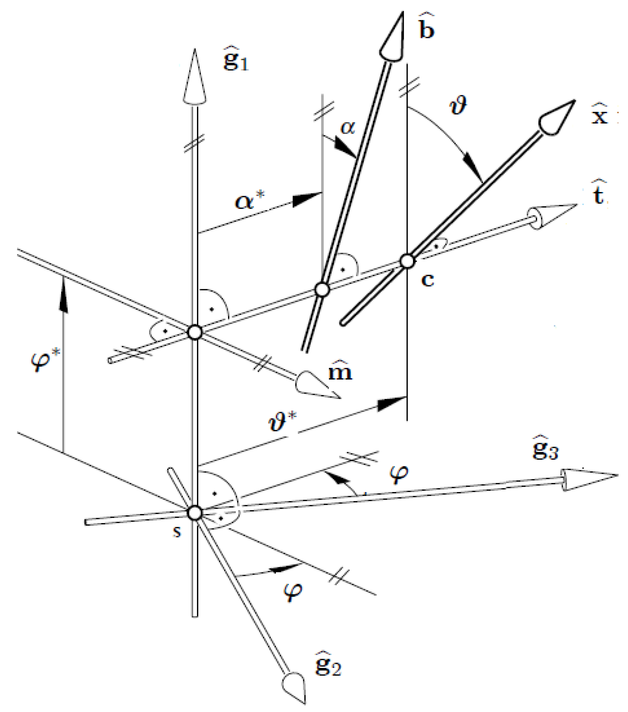
Notice that the striction point is the origin of the auxiliary Blaschke frame; that is, (see Figure 2) (compared with [1,2,3,4,5]). This means that , and
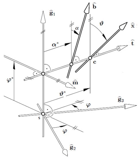
Figure 2.
and its Disteli-axis .
3.1. Disteli Formulae for a Spacelike Line Trajectory
The formula confirms the connections through the -axis of the line trajectories for one-parameter spatial locomotion [1,2,3,4,5]. There are many works which consider the formulae and geometric invariants of ruled surfaces [9,10,11,12,13,14,15,24,25,26,27,28]. The Lorentzian formulae may be gained immediately from the dual spherical curvature of as follows: Substituting the Equation (22) into Equation (20), we have
Equation (24) is the Lorentzian dual version of the equation for a point trajectory in planar and spherical locomotions in form (see [1,2,3,4]). From the real and the dual parts, respectively, we get:
and
Equation (25) simultaneously with (26) are the formulae of a line trajectory in spatial Lorentzian locomotions. Its geometrical importance is shown in Figure 2. Equation (25) offers the connection among the attitudes of in the -space and its -axis . Equation (26) offers the distance from to . The sign of (+ or −) in the above expression indicates that the attitudes of the -axis are situated on the positive or negative direction of the central normal of at , while the direction of is located by
However, we can express a second dual version of the equation by applying dual angle estimations. This means we seek the steady line , which is at a steady dual angle from a steady line . So, we set the central dual angle of the dual unit vectors , and
such that and stay steady up to the second order at ; that is,
and
We have for the first order, steady
and, for the second order, steady
Then, will be invariant in the second estimation if, and only if, is the -axis of ; that is,
Substituting Equation (6) into Equation (27), we have
From Equations (23) and (28), one finds that:
Substituting Equation (22) into Equation (29), we may express the equation as:
By considering the real and dual parts, we obtain the following:
and
The Equations (31) with (32) are the formulae of a line trajectory in spatial Lorentzian locomotions. Via Figure 2, the sign of (+ or −) in Equation (32) references that the attitudes of the axis are settled on the positive or negative direction on the shared . Since the central points of the line’s trajectories are on the normal plane, when the direction of their rulings are settled by , the -formulae can be settled in the plane . Hence, any arbitrary point on this plane is the central point of the oriented line and the radius can be acquired by Equation (31). However, the central point may be on if , and on the if . In the second condition the point can be gained by putting in Equation (31), which can be reduced as follows:
Equation (33) represents a linear equation in the and of the -axis . The position of line L will change if the parameter is assigned a different value, while keeping steady. However, if a pencil of the steady line envelope is a curve on the plane , then, the subspace modifies if the parameter of a line has distinct values, but steady. Therefore, the pencil of all steady lines L shown by Equation (33) is a line congruence for all values of . The results indicate a straightforward geometric illustration of the properties of the formulae for a steady linear trajectory.
At the conclusion of this subsection, we are able to consider the equation for the axodes, in the following manner: Substituting , , and , and into Equation (30), after simplification, it may be deduced that we obtain,
3.2. Spacelike Torsion Line Congruence
We now locate the torsion line congruence, which is the spatial symmetry of the Lorentzian circling-point dual curve (cubic of steady curvature) [1,2,3,4,5].
Definition 1.
The trajectory of the dual points, whose trajectories have a vanishing dual torsion in , is named the Lorentzian circling-point curve or the cubic of steady curvature.
The dual curve in with zero torsion is a planar section of . The Lorentzian cone with steady curvature can be defined as the trace of dual points in that possess trajectories with a steady osculating dual plane. By utilizing Definition 1 and Equation (21), we obtain
Therefore, the spatial symmetry of the torsion dual cone with steady curvature is defined by: (1) The line complex pointed by the torsion cone , and (2) the line complex pointed by the linked plane of lines . All the pencil of lines -space and also in the plane satisfy initiating the torsion line congruence. Therefore, the torsion line congruence is traced by a pencil of planes , each of which is coupled with an orientation of the torsion cone c. Therefore, we present the following theorem:
Theorem 3.
Through the locomotion , set the pencil of steady lines of the movable axode, such that each one of these lines has symmetry of a torsion dual cone with steady curvature. Then, this pencil of lines defines a torsion line congruence, which are the shared lines of the two line complexes and .
Furthermore, from Equation (21), we have:
This shows that , and . In this case, the -axis is steady up to the second order, and the line moves over it with steady pitch. Hence, the ruled surface is formed by a line that exists at a steady Lorentzian distance and a steady Lorentzian angle relative to the -axis .
Theorem 4.
A torsion line congruence is a steady -axis if, and only if, = steady, and = steady.
However, if we set Equations (21) and (22), we attain the spatial symmetry of the torsion dual cone with steady curvature as
We solve Equation (37) for as
where
The real part of Equation (38) characterizes the Lorentzian cone for the spherical part of the locomotion and is
A Lorentzian spherical curve is produced by the intersection of the torsion cone with a Lorentzian unit sphere fixed at the cone’s apex. Associated with the orientation of a line L in the torsion cone, there exists a plane defined by the dual part of Equation (38). This plane is
For any orientation of a line L within the torsion cone, there exists a corresponding plane consisting of lines that are parallel to L. The torsion cone and the plane of lines is used to define the torsion line congruence.
3.3. Line Geometry of the Spacelike Torsion Line Congruence
In order to recognize the torsion line congruence, from the real and the dual parts of Equation (22), respectively, we get:
and
Let be the director surface of the congruence; that is, . After some algebraic manipulations, it can be determined that
Let be a point on the directed line . We can write:
If we set and as the locomotion parameter, then is a ruled in -space. By substituting the Equation (40) into the Equation (42), we find
which is the Lorentzian spherical torsion curve. From Equations (44)–(46), we also obtain that:
According to Equations (46) and (47), we have:
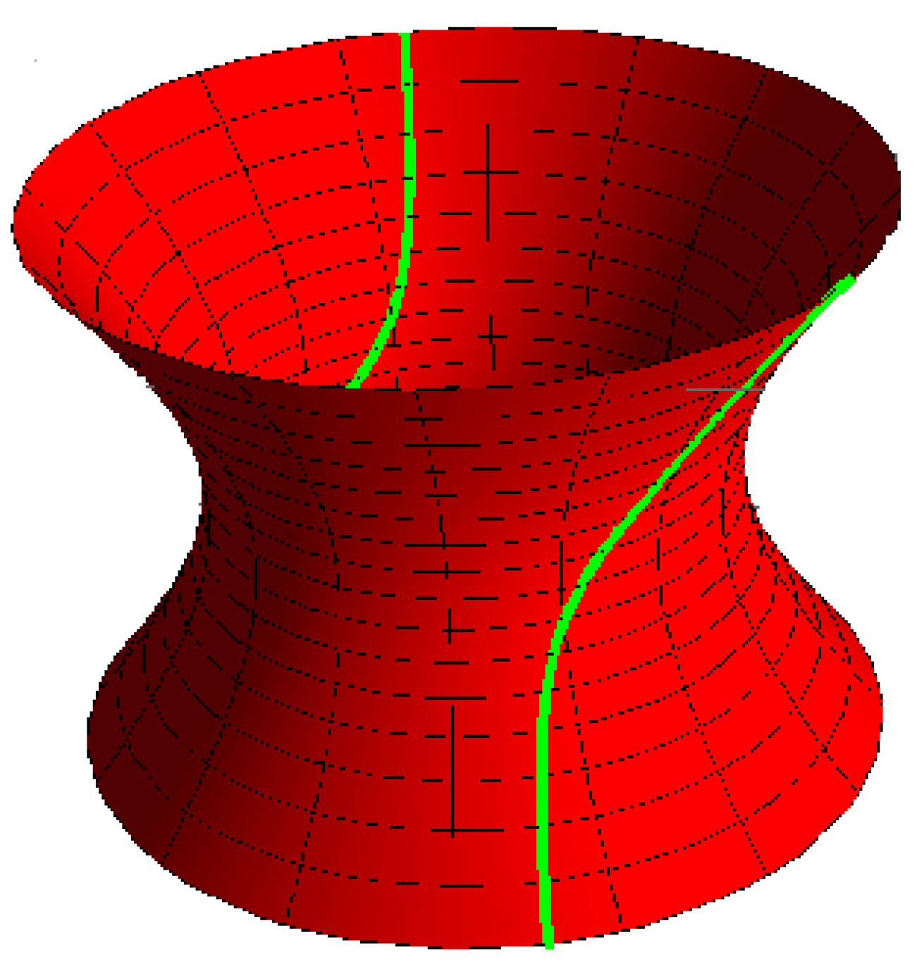
- (1)
- Lorentzian spherical torsion curve with its torsion ruled surface: for , , , , (Figure 3 and Figure 4).
 Figure 3. Lorentzian torsion curve.
 Figure 4. torsion ruled surface.
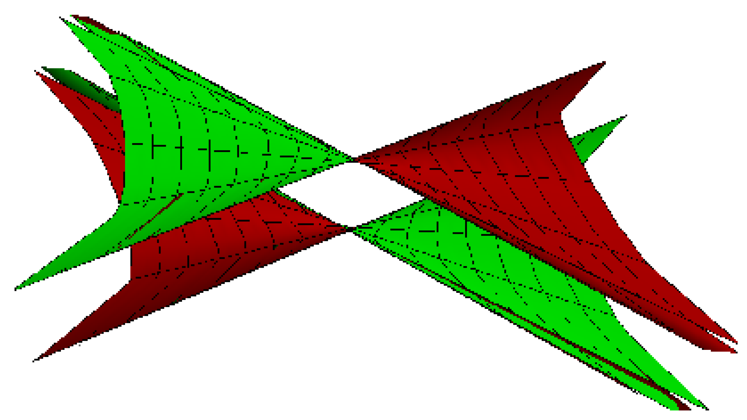
 - (2)
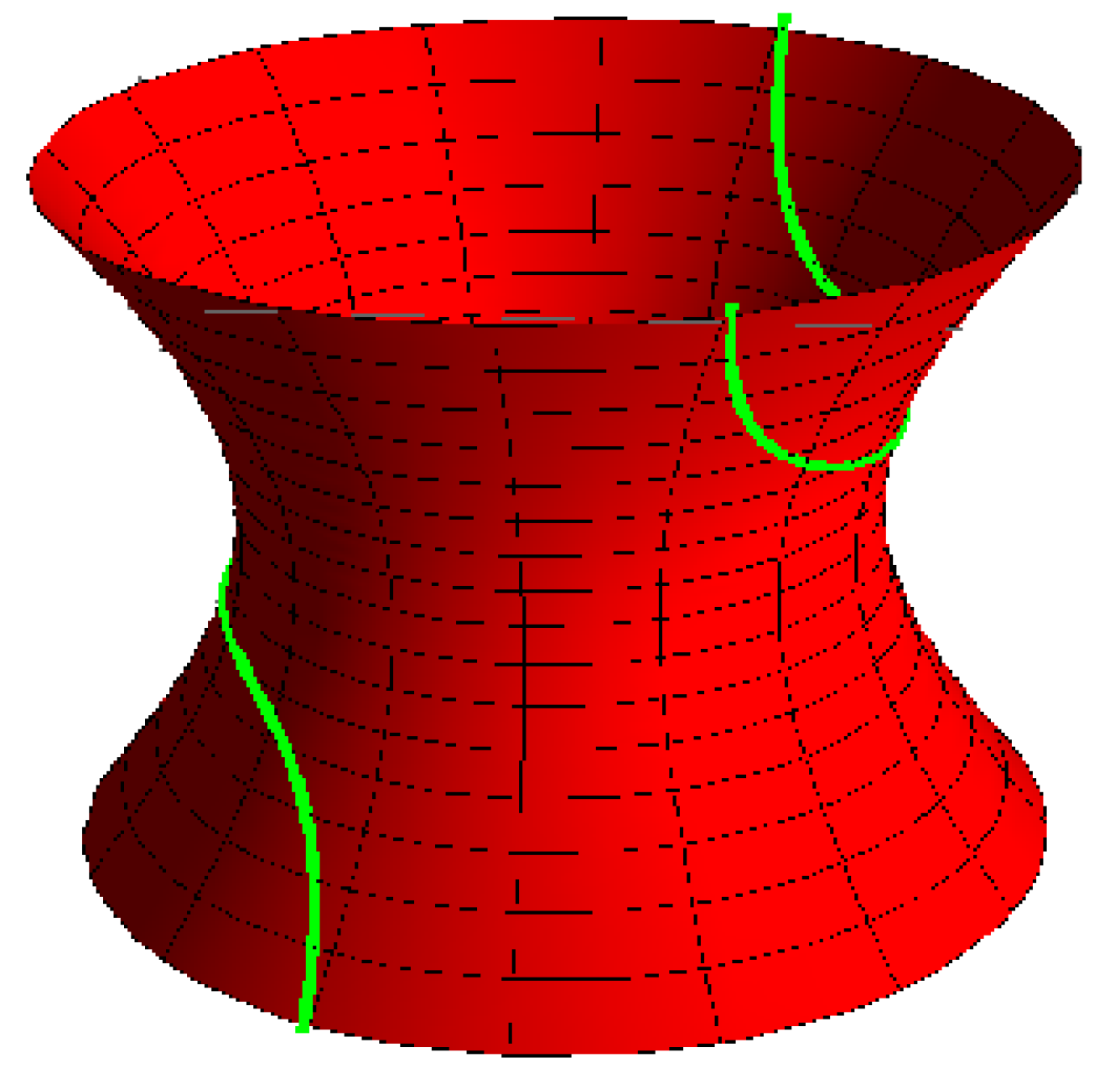
- Lorentzian spherical torsion curve with its torsion ruled surface: for , , , , (Figure 5 and Figure 6).
 Figure 5. Lorentzian torsion curve.
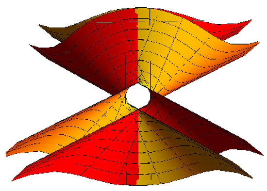 Figure 6. torsion ruled surface.
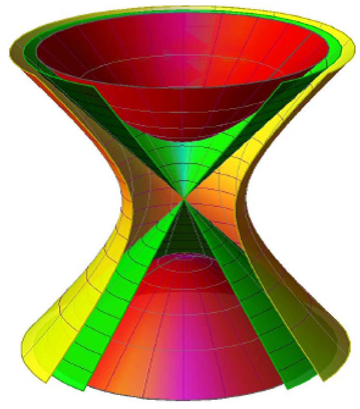
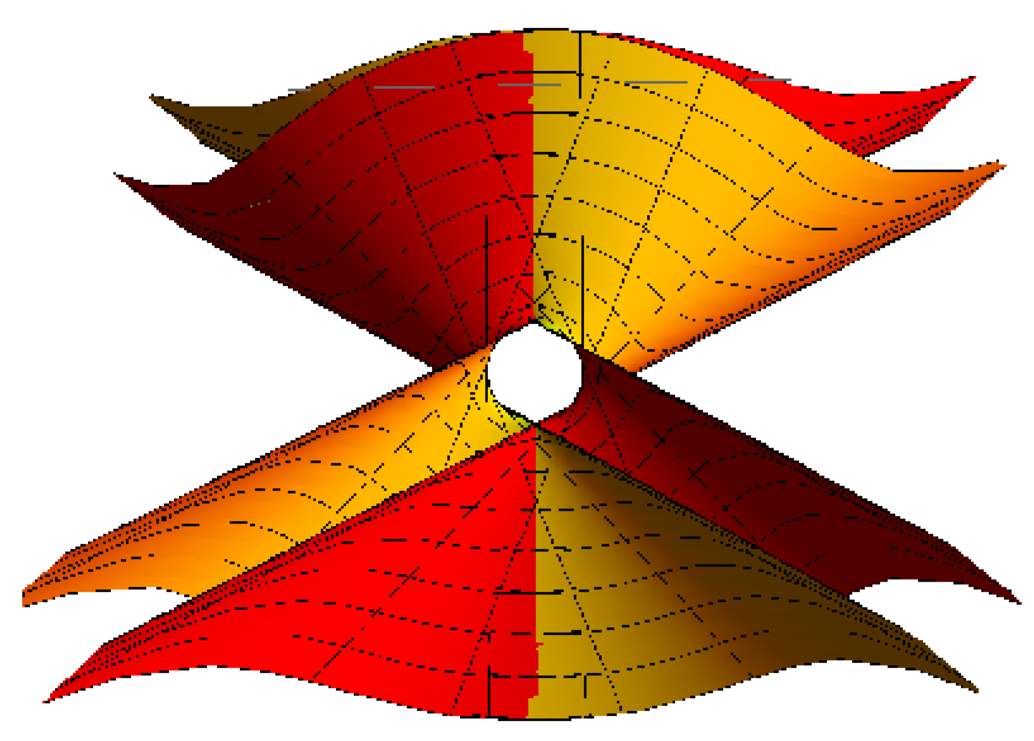
 - (3)
- Lorentzian spherical torsion curve with its torsion ruled surface: for , , , , (Figure 7 and Figure 8).
 Figure 7. Lorentzian torsion curve.
 Figure 8. torsion ruled surface.
4. Conclusions
The main outcome of the paper is generalization of the and formulae in the Lorentzian motion. On the basis of the E. Study map, formulae for the velocity and acceleration of a dual curve are obtained by applying the invariants of relative locomotion through two Lorentzian spheres. The torsion and curvature of this curve are related to the invariants. The equation and the equation are then given novel proofs using the axode invariants. Additionally, the well-known torsion cone with a constant spherical kinematic curvature is investigated in dual space. Further, we defined and studied torsion line congruence. Then, a detailed examination of a Lorentzian torsion line congruence and its spatial equivalent was performed using the E. Study map. It is possible to discuss specific issues and develop new implementations using the E. Study map to describe spatial kinematics in Minkowski 3-space (). As seen in [9,12,17,20,21,26], in the future, our primary focus will be on the development of ruled surfaces to serve as tooth edges for gears with skew axes.
Author Contributions
Conceptualization, R.A.A.-B. and A.A.A.; methodology, R.A.A.-B. and A.A.A.; software, R.A.A.-B. and A.A.A.; validation, R.A.A.-B.; formal analysis, R.A.A.-B. and A.A.A.; investigation, R.A.A.-B. and A.A.A.; resources, R.A.A.-B.; data curation, R.A.A.-B. and A.A.A.; writing—original draft preparation, R.A.A.-B. and A.A.A.; writing—review and editing, A.A.A.; visualization, R.A.A.-B. and A.A.A.; supervision, R.A.A.-B.; project administration, R.A.A.-B.; funding acquisition, A.A.A. All authors have read and agreed to the published version of the manuscript.
Funding
This research was funded by Princess Nourah bint Abdulrahman University Researchers Supporting Project number (PNURSP2023R337).
Data Availability Statement
Our manuscript has no associated data.
Acknowledgments
The authors would like to acknowledge the Princess Nourah bint Abdulrahman University Researchers Supporting Project number (PNURSP2023R337), Princess Nourah bint Abdulrahman University, Riyadh, Saudi Arabia.
Conflicts of Interest
The authors declare that there are no conflict of interest regarding the publication of this paper.
References
- Bottema, O.; Roth, B. Theoretical Kinematics; North-Holland Press: New York, NY, USA, 1979. [Google Scholar]
- Karger, A.; Novak, J. Space Kinematics and Lie Groups; Gordon and Breach Science Publishers: New York, NY, USA, 1985. [Google Scholar]
- Schaaf, J.A. Curvature Theory of Line Trajectories in Spatial Kinematics. Ph.D. Thesis, University of California, Davis, CA, USA, 1988. [Google Scholar]
- Stachel, H. Instantaneous Spatial Kinematics and the Invariants of the Axodes; Technical Report; Institute fur Geometrie, TU Wien: Wien, Austria, 1996. [Google Scholar]
- Pottman, H.; Wallner, J. Computational Line Geometry; Springer: Berlin/Heidelberg, Germany, 2001. [Google Scholar]
- Garnier, R. Cours de Cinématique, Tome II: Roulement et Vibration-La Formule de Savary et son Extension a l’Espace; Gauthier-Villars: Paris, France, 1956. [Google Scholar]
- Phillips, J.; Hunt, K. On the theorem of three axes in the spatial motion of three bodies. J. Appl. Sci. 1964, 15, 267–287. [Google Scholar]
- Skreiner, M. A study of the geometry and the kinematics of Instantaneous spatial motion. J. Mech. 1966, 1, 115–1439. [Google Scholar] [CrossRef]
- Dizioglu, B. Einfacbe Herleitung der Euler-Savaryschen Konstruktion der riiumlichen Bewegung. Mech. Mach. Theory 1974, 9, 247–254. [Google Scholar] [CrossRef]
- Abdel-Baky, R.A.; Al-Solamy, F.R. A new geometrical approach to one-parameter spatial motion. J. Eng. Math. 2008, 60, 149–172. [Google Scholar] [CrossRef]
- Sprott, K.; Ravani, B. Cylindrical milling of ruled surfaces. Int. J. Adv. Manuf. Technol. 2008, 38, 649–656. [Google Scholar] [CrossRef]
- Figliolini, G.; Stachel, H.; Angeles, J. The Computational fundamentals of spatial cycloidal gearing. In Computational Kinematics, Proceedings of the 5th International Workshop on Computational Kinematics; Kecskeméthy, A., Müller, A., Eds.; Springer: Berlin/Heidelberg, Germany, 2009; pp. 375–384. [Google Scholar]
- Abdel-Baky, R.A.; Al-Ghefari, R.A. On the one-parameter dual spherical motions. Comput. Aided Geom. Des. 2011, 28, 23–37. [Google Scholar] [CrossRef]
- Al-Ghefari, R.A.; Abdel-Baky, R.A. Kinematic geometry of a line trajectory in spatial motion. J. Mech. Sci. Technol. 2015, 29, 3597–3608. [Google Scholar] [CrossRef]
- Abdel-Baky, R.A. On the curvature theory of a line trajectory in spatial kinematics. Commun. Korean Math. Soc. 2019, 34, 333–349. [Google Scholar]
- Gungor, M.A.; Ersoy, S.; Tosun, M. Dual Lorentzian spherical movements and dual Euler-Savary formula. Eur. J. Mech.-A/Solids 2009, 28, 820–826. [Google Scholar] [CrossRef]
- Ayyilidiz, N.; Yalin, S.N. On instantaneous invariants in dual Lorentzian space kinematics. Arch. Mech. 2010, 62, 223–238. [Google Scholar]
- Zhang, X.; Zhang, J.; Pang, B.; Zhao, W. An accurate prediction method of cutting forces in 5-axis flank milling of sculptured surface. Int. J. Mach. Tools Manuf. 2016, 104, 26–36. [Google Scholar] [CrossRef]
- Calleja, A.; Bo, P.; Gonzalez, H.; Barton, M.; Norberto, L.; de Lacalle, L. Highly accurate 5-axis flank CNC machining with conical tools. Int. J. Adv. Manuf. Technol. 2018, 97, 1605–1615. [Google Scholar] [CrossRef]
- Gonzãlez, H.; Pereira, O.; López de Lacalle, L.N.; Calleja, A.; Ayesta, I.; Munoxax, J. Flank-Milling of Integral Blade Rotors Made in Ti6Al4V Using Cryo CO2 and Minimum Quantity Lubrication. J. Manuf. Sci. Eng. 2021, 143, 091011-2. [Google Scholar] [CrossRef]
- Hamdi, M.; Aifaoui, N.; Abdelmajid, B. Idealization of cadgeometry using design and analysis integration features models. In Proceedings of the ICED 2007, the 16th International Conference on Engineering Design, Paris, France, 28–31 July 2007. [Google Scholar]
- Rezayat, M. Midsurface abstraction from 3d solid models: General theory and applications. Comput. Aided Des. 1996, 28, 905–915. [Google Scholar] [CrossRef]
- Ferhat, T.; Abdel-Baky, R.A. On a spacelike line congruence which has the parameter ruled surfaces as principal ruled surfaces. Int. Electron. J. Geom. 2019, 12, 135–143. [Google Scholar]
- Abdel-Baky, R.A.; Unluturk, Y. A new construction of timelike ruled surfaces with constant Disteli-axis. Honam Math. J. 2020, 42, 551–568. [Google Scholar] [CrossRef]
- Alluhaibi, N.; Abdel-Baky, R.A. On the one-parameter Lorentzian spatial motions. Int. J. Geom. Methods Mod. Phys. 2019, 16, 1950197. [Google Scholar] [CrossRef]
- Alluhaibi, N.; Abdel-Baky, R.A. On the kinematic-geometry of one-parameter Lorentzian spatial movement. Int. J. Adv. Manuf. Technol. 2022, 121, 7721–7731. [Google Scholar] [CrossRef]
- O’Neil, B. Semi-Riemannian Geometry Geometry, with Applications to Relativity; Academic Press: New York, NY, USA, 1983. [Google Scholar]
- Walfare, J. Curves and Surfaces in Minkowski Space. Ph.D. Thesis, K.U. Leuven, Faculty of Science, Leuven, Belgium, 1995. [Google Scholar]
Disclaimer/Publisher’s Note: The statements, opinions and data contained in all publications are solely those of the individual author(s) and contributor(s) and not of MDPI and/or the editor(s). MDPI and/or the editor(s) disclaim responsibility for any injury to people or property resulting from any ideas, methods, instructions or products referred to in the content. |
© 2023 by the authors. Licensee MDPI, Basel, Switzerland. This article is an open access article distributed under the terms and conditions of the Creative Commons Attribution (CC BY) license (https://creativecommons.org/licenses/by/4.0/).