Article

Robust Fault Estimation and Tolerant Control for Uncertain Takagi–Sugeno Fuzzy Systems

1
Department of Computer Engineering and Networks, College of Computer and Information Sciences, Jouf University, Sakaka 72388, Saudi Arabia
2
Control and Energy Management Laboratory, National School of Engineering, Sfax University, Sfax 3038, Tunisia
*
Author to whom correspondence should be addressed.
Symmetry 2023, 15(10), 1894; https://doi.org/10.3390/sym15101894
Submission received: 16 September 2023 / Revised: 2 October 2023 / Accepted: 8 October 2023 / Published: 9 October 2023

Abstract

:
This research addresses the intricate challenges of fault estimation (FE) and fault-tolerant control (FTC) within a specific subset of T-S fuzzy systems. These systems are characterized by their localized nonlinear models, the presence of unknown inputs, actuator imperfections, and disruptive output disturbances, making them fertile ground for exploration in this study. The contributions of this paper can be summarized as follows: (1) First, we employ coordinate transformation matrices to convert the T-S fuzzy model. This transformation separates the unknown inputs and disturbances at the output. Subsequently, we equip the modified system with a T-S fuzzy adaptive sliding mode observer (ASMO) that serves the dual purpose of fortifying resilience against disruptions and adeptly deducing an extensive spectrum of fluctuating actuator failure signals. (2) In the next step, the insights gained from FE are harnessed to craft a dynamic fuzzy output feedback fault-tolerant controller (DOFFTC). This controller aims to mitigate the effects of actuator errors to maintain the stability of the closed-loop system. The article creates the necessary conditions for the presence of the required ASMO and DOFFTC using H-infinity filtering methods. To address the optimization issue posed by these criteria, we utilize linear matrix inequalities (LMIs) and calculate the required gains for implementation using convex optimization techniques. (3) The study concludes by illustrating the applicability of the proposed techniques with an example employing an inverted pendulum. This paper presents a comprehensive approach to overcoming the challenges of FE and FTC within T-S fuzzy systems. It leverages precise mathematical formulations and optimization strategies to achieve resilient and dependable control, even when confronted with intricate system dynamics.

1. Introduction

In practical applications, a prevalent challenge arises from the substantial nonlinearities inherent in most physical systems. A valuable approach to approximating these nonlinear dynamics is the utilization of Takagi–Sugeno (T-S) fuzzy models, which smoothly blend a set of linear models [1]. Through the utilization of T-S fuzzy models, the intricate matters of assessing stability and devising control strategies for nonlinear systems can be skillfully tackled by adopting a perspective rooted in the principles of linear system theory. An extensive body of work has emerged in the literature, spanning from [2,3,4,5,6,7], exploring the stability analysis and control synthesis areas inside the T-S fuzzy systems domain.
With the growing demand for high-performance systems, the components crucial for system operation, such as actuators, sensors, and control units, may succumb to faults during their operation. These faults disrupt the regular functioning of the system and consequently lead to undesirable performance outcomes when utilizing design controllers. This necessitates the implementation of suitable compensatory measures to safeguard reliability and safety. To fulfill this imperative, the fields of fault estimation (FE) and fault-tolerant control (FTC) have garnered significant attention within the past decade, as documented in References [8,9,10,11,12]. Various classes of robust observers have been developed for T-S models, encompassing adaptive observers [13,14,15], sliding mode observers (SMOs) [16,17,18,19,20,21], and unknown input observers (UIOs) [22,23,24], among others.
Given the constraint of only having access to system outputs for control purposes, an observer-based DOFFTC framework was introduced to address the occurrence of faults by implementing fault compensation strategies. For T-S fuzzy models affected by actuator defects and external disturbances, a fuzzy DOFFTC is examined in [6], along with the derivation of special requirements stated as linear matrix inequalities (LMIs). As system complexity grows, an observer-based DOFFTC is further advanced in [25] to accommodate T-S fuzzy systems challenged by parameter uncertainties, external disturbances, and intermittent actuator faults. The developed observer incorporates H performance to ensure robustness against disturbances.
The research landscape extends to the investigation of FE and DOFFTC for discrete-time T-S fuzzy systems with time-varying delays and actuator faults in [26], albeit solely focusing on actuator faults. The focus is widened in [27] to include time-varying delays, outside disturbances, as well as actuator and sensor defects in T-S fuzzy systems. In this research, we introduce an upgraded fuzzy observer tailored to tackle the challenges of FE and DOFFTC. Additionally, we delve into the realm of robust SMO solutions, specifically tailored for T-S fuzzy systems wherein unobservable premise variables are vulnerable to potential actuator and sensor inaccuracies, as expounded in [28]. By examining the corresponding output error injection required to sustain sliding motion, these faults are calculated. A DOFFTC is created using this estimation information to lessen the effects of failures and guarantee system stability. The complexity of nonlinear systems increases along with the number of fuzzy rules, which makes stability analysis more difficult. This is addressed by a method described in [29] that uses extended T-S models to cut down on the number of rules needed to characterize the system. Another approach is suggested in [30,31,32], which maintains sector-bounded criteria while allowing extra nonlinear elements in the fuzzy system description. As a result, fewer rules are needed without sacrificing model correctness.
It is to be noted that the primary differentiator of T-S (Takagi–Sugeno) fuzzy systems, which makes them particularly suited for our proposed method, lies in their ability to approximate complex nonlinear systems using a set of local linear models. Unlike many other modeling approaches that rely on global linearizations or purely nonlinear models, T-S fuzzy systems excel at capturing the local behavior of a system. This property is essential in dealing with localized nonlinear models, which are a characteristic feature of the systems we address in this study.
Moreover, T-S fuzzy systems inherently provide a framework for adaptive control and fault estimation due to their rule-based structure. This allows us to seamlessly integrate our adaptive sliding mode observer (ASMO) and dynamic fuzzy output feedback fault-tolerant controller (DOFFTC) into the system’s existing rule base, enhancing its ability to handle actuator failures and output disturbances effectively.
By highlighting the unique advantages of T-S fuzzy systems, we aim to emphasize why they are the ideal choice for implementing our proposed method, which is tailored to address the specific challenges posed by systems characterized by localized nonlinear models, unknown inputs, actuator imperfections, and disruptive output disturbances.
To the best of our knowledge, a thorough investigation of the complex problems of FE and FTC for continuous-time T-S fuzzy systems with sector-bounded functions, unknown inputs, measurement disturbances, and actuator defects has not been conducted. The present study was motivated by this information gap. This paper’s main contributions may be summed up as follows:
  • The study of FE and DOFFTC for T-S fuzzy systems with local nonlinear models, unknown inputs, output disturbances, and actuator defects is pioneered in this research.
  • By harnessing the capabilities of adaptive observers in conjunction with the sliding mode technique, we engineer an ASMO. This innovative ASMO is designed to swiftly appraise actuator malfunctions and bolster resilience against disruptive influences. An FE algorithm, comprising a proportional output vector and an integral component, is subsequently introduced to improve FE speed and accuracy.
  • Through the application of H performance criteria, new sufficient conditions for the existence of the desired observer and controller are derived and presented as a convex optimization problem based on LMIs.
  • Notably, the ASMO and DOFFTC controllers are designed independently, a design approach that conveniently reduces computational complexity.
In the realm of control systems engineering, the need for fault estimation and fault-tolerant control solutions has grown considerably with the increasing complexity of real-world systems. However, when it comes to T-S fuzzy systems with local nonlinear models, unknown inputs, actuator defects, and output disturbances, there exists a distinct set of challenges that require innovative solutions. This paper embarks on a journey to address these challenges head-on by providing a comprehensive framework for robust adaptive sliding mode observer-based fault estimation and tolerant control. In doing so, we aim to bridge the gap in the existing literature, which often falls short in providing effective solutions for this particular class of T-S fuzzy systems. By enhancing resilience against disturbances and rapidly estimating a wide range of time-varying actuator failure signals, we seek to pave the way for more robust and stable control in the face of complex system dynamics.
In summary, this research explores FE and FTC extensively within the context of T-S fuzzy systems, tackling a wide range of issues pertaining to fault compensation and system stability in the face of intricate nonlinearities and various fault situations.
Navigating the intricacies of our research is akin to embarking on a well-guided journey. In Section 2, “System Description”, we set the stage by introducing the foundation of T-S fuzzy systems with local nonlinear models, a key stepping stone to grasp the challenges ahead. As we delve deeper, Section 3, “Main Results”, serves as our compass. Here, we take you through a meticulously crafted path, beginning with the state transformation (Section 3.1) that paves the way for robust ASMO design (Section 3.2). The journey continues with stability analysis (Section 3.3) and sliding motion reachability (Section 3.4), where we unravel the secrets to resilient control. Just as a seasoned traveler anticipates the next destination, we invite you to explore Section 4, where we unveil the fault-tolerant controller design. Finally, in Section 5, you will witness our approach in action through a compelling real-world example. As with the closing chapter of a gripping novel, Section 6, “Conclusion”, ties it all together. Therefore, fasten your seat belt and embark on this intellectual odyssey, where each section is a carefully crafted milestone on your way to mastering fault estimation and tolerant control in T-S fuzzy systems.

2. System Description

Let us consider a continuous-time T-S fuzzy system with local nonlinear components, which can be described using fuzzy IF–THEN rules. Each rule, denoted as Rule i, takes the following form:
Rule i: IF α 1 is π i 1 , α 2 is π i 2 , and so on until α g is π i g , THEN the system dynamics are described by the following equations:
x ˙ = A i x + N i φ ( x ) + B i u + F i f a + E d y = C x + D ω
In these equations:
  • x R n represents the state vector.
  • u R m is the input.
  • y R p is the measurable output.
  • f a R q denotes an additive actuator fault.
  • d R d represents the disturbance input or uncertainties.
  • ω R l is a disturbance in the measurement output equation.
  • φ ( x ) R j is a known nonlinear function.
  • Both d and ω belong to the space of square integrable functions denoted as L 2 0 , .
  • The matrices A i R n × n , N i R n × j , B i R n × m , F i R n × q , E R n × d , C R p × n , and D R n × l ( p l ) are matrices of real constant with the proper dimensions.
Several assumptions are made:
  • Matrix E and D both being of full column rank.
  • The pairs ( A i , B i ) are controllable.
  • The pairs ( A i , C ) are observable.
  • α = α 1 , α g is the premise variables vector.
  • π i j ( i = 1 , , k , j = 1 , g ) represents the fuzzy sets.
  • The quantity of IF–THEN rules is k, and the quantity of premise variables is g.
The following is the expression for the global fuzzy model created by combining each individual plant rule:
x ˙ = i = 1 k ρ i α A i x + N i φ ( x ) + B i u + F i f a + E d y = C x + D ω
Here, ρ i ( α ) is the blending weight, defined as σ i ( α ) i = 1 k σ i ( α ) , and σ i α = j = 1 g π i j α is the membership function. π i j ( · ) represents the degree of membership of α in the fuzzy set π i j . We assume that σ i ( α ) 0 for i = 1 , , k . It is evident that ρ i ( α ) 0 for i = 1 , , k , and i = 1 k ρ i ( α ) = 1 .
To present the main results, we introduce certain assumptions and lemmas.
Hypothesis 1. 
The rank of the product of matrices C and E is equal to the rank of matrix E.
Hypothesis 2. 
For any complex number s with a non-negative real part, the rank of the block matrix
r a n k s I n A i E C 0
is equal to n + l , for all i in the range from 1 to k.
Hypothesis 3. 
The disturbance input d, the actuator fault f a , and its derivative satisfy the following bounded constraints:
  • The norm of d is less than or equal to ρ d .
  • The norm of f a is less than or equal to ρ a .
  • The norm of the derivative of f a is less than or equal to ρ a a .
Here, ρ d , ρ a , and ρ a a are known positive constants.
Hypothesis 4. 
We assume that the function φ ( x ) is a Lipschitz function bounded within a cone sector. It satisfies the following conditions:
  • φ T ( x ) φ ( x ) R x 0 , where R is a constant vector with appropriate dimensions.
  • The difference between φ ( x ) and φ ( x ^ ) in terms of norm is bounded by γ times the difference between x and x ^ , where γ represents the Lipschitz constant.
Lemma 1 ([33]). 
For any matrices (or vectors) X and Y with appropriate dimensions, there exists an arbitrary scalar ε > 0 such that the following inequality holds:
X T Y + Y T X ε X T X + ε 1 Y T Y
Lemma 2 ([34]). 
For given matrices U and V with suitable dimensions, there exists a matrix P > 0 such that the following inequality is satisfied:
U T V + V T U U T P U + V T P 1 V
Lemma 3 ([35]). 
If we have
  • Λ i i < 0 for 1 i k and
  • 2 k 1 Λ i i + Λ i j + Λ j i < 0 for 1 i < j k
then we can conclude that:
i = 1 k j = 1 k ρ i ( α ) ρ j ( α ) Λ i j < 0
In accordance with Chilali (1996), as stated in [36], it is established that when a matrix A of dimensions n × n is considered, the eigenvalues of A can be found residing within a circular region, denoted as D ( α , τ ) . This circular region is centered at coordinates ( α , 0 ) and exhibits a radius of τ . This remarkable characteristic holds true under the condition that a matrix P > 0 of dimensions n × n exists, such that the subsequent matrix demonstrates negative definiteness:
α P τ P + P A τ P + ( P A ) T α P < 0

3. Main Results

In this part, we unveil the central findings of our study, encompassing the metamorphosis of states and the birth of a novel fuzzy system. Additionally, we furnish prerequisites for conceiving an ASMO and a DOFFTC, delineated in the language of LMIs.

3.1. State Transformation

As demonstrated in [37], assuming Hypothesis 1 holds, we can establish coordinate transformations z = T x and η = S y , where T R n × n and S R p × p , such that the system described by Equation (2) can be expressed in the following form:
z ˙ = i = 1 k ρ i α A ¯ i z + N ¯ i φ ( x ) + B ¯ i u + F ¯ i f a + E ¯ d η = C ¯ z + D ¯ ω
Here, the matrices A ¯ i , N ¯ i , B ¯ i , F ¯ i , E ¯ , C ¯ , and D ¯ are defined as follows:
A ¯ i = T A i T 1 = A i , 11 A i , 12 A i , 21 A i , 22 , N ¯ i = T N i = N i , 1 N i , 2 , B ¯ i = T B i = B i , 1 B i , 2 , F ¯ i = T F i = F i , 1 F i , 2 , E ¯ = T E = E 1 0 , C ¯ = S C T 1 = C 1 0 0 C 2 , D ¯ = S D = 0 D 2
Here, A i , 11 R d × d , B i , 1 R d × m , N i , 1 R d × j , E 1 R d × d , F i , 1 R d × q , C 1 R d × d , C 2 R ( p d ) × ( n d ) , D 2 R ( p d ) × l , and C 1 is a nonsingular matrix, while E 1 has full column rank.
The equation denoted as (6) allows us to delve deeper into the system’s structure, leading to its breakdown in the subsequent
z ˙ 1 = i = 1 k ρ i α A i , 11 z 1 + A i , 12 z 2 + N i , 1 φ ( x ) + B i , 1 u + F i , 1 f a + E 1 d η 1 = C 1 z 1 z ˙ 2 = i = 1 k ρ i α A i , 21 z 1 + A i , 22 z 2 + N i , 2 φ ( x ) + B i , 2 u + F i , 2 f a η 2 = C 2 z 2 + D 2 ω
where z = c o l z 1 , z 2 with z 1 R d and η = c o l η 1 , η 2 with η 1 R d .

3.2. ASMO Design

In the following section, we embark on the journey of crafting an ASMO nestled within the realms of fuzzy systems. The ASMO unfolds its design in the subsequent fashion:
z ^ ˙ 1 = i = 1 k ρ i α A i , 11 z ^ 1 + A i , 12 z ^ 2 + N i , 1 φ ( x ^ ) + B i , 1 u + L i , 11 e η 1 + ϑ η ^ 1 = C 1 z ^ 1 z ^ ˙ 2 = i = 1 k ρ i α A i , 21 z ^ 1 + A i , 22 z ^ 2 + N i , 2 φ ( x ^ ) + B i , 2 u + F i , 2 f ^ a + L i , 21 e η 1 + L i , 22 e η 2 η ^ 2 = C 2 z ^ 2 f ^ ˙ a = Γ i = 1 k ρ i α K i e ˙ η 2 + σ e η 2
Here, z ^ and η ^ represent the estimates of z and η , respectively. e η 1 = η 1 η ^ 1 and e η 2 = η 2 η ^ 2 . The matrices L i , 11 , L i , 21 , L i , 22 , and K i are the observer gains that are designed later. f ^ a represents the estimated actuator fault. The matrix Γ > 0 corresponds to the learning rate, and σ is a positive scalar.
The discontinuous term ϑ is defined as follows:
ϑ = κ P 1 C 1 1 e η 1 P 1 C 1 1 e η 1 , e η 1 0 0 , otherwise
Here, the design scalar κ is a positive value that is discussed in subsequent sections.
Let us define some error terms to simplify the analysis:
  • e z 1 = z 1 z ^ 1 , where e z 1 is related to the error in z 1 and z ^ 1 .
  • e z 2 = z 2 z ^ 2 , where e z 2 is related to the error in z 2 and z ^ 2 .
  • e f a = f a f ^ a , where e f a represents the error in the actuator fault estimation.
  • e φ ( x ) = φ ( x ) φ ( x ^ ) , which reflects the error in the nonlinear function φ .
Now, let us introduce a matrix L ¯ i defined as:
L ¯ i = Δ L i , 11 0 L i , 21 L i , 22
If we choose L i , 11 and L i , 21 as follows:
  • L i , 11 = ( A i , 11 A 11 s ) C 1 1 , where A 11 s is an arbitrary negative definite matrix.
  • L i , 21 = A i , 21 C 1 1 .
Then the error dynamics can be described as follows:
e ˙ z 1 = i = 1 k ρ i α A 11 s e z 1 + A i , 12 e z 2 + N i , 1 e φ ( x ) + F i , 1 f a + E 1 d ϑ
e ˙ z 2 = i = 1 k ρ i α A i , 22 L i , 22 C 2 e z 2 + N i , 2 e ϕ ( x ) + F i , 2 e f a L i , 22 D 2 ω
Lemma 4 ([38]). 
The pair ( A i , 22 , C 2 ) is detectable for any i = 1 , 2 , k if and only if Hypothesis 2 holds.
Remark 1. 
From Lemma 4, we can conclude that there exists a matrix L i , 22 for any i = 1 , 2 , k , such that A i , 22 L i , 22 C 2 is stable.
The evolution of the error in fault estimation follows this equation:
e ˙ f a = f ˙ a f ^ ˙ a = f ˙ a Γ i = 1 k ρ i α K i e ˙ η 2 + σ e η 2 = f ˙ a Γ i = 1 k j = 1 k ρ i α ρ j α K i C 2 A j , 22 L j , 22 C 2 e z 2 + K i C 2 N j , 2 e ϕ ( x ) + K i C 2 F j , 2 e f a K i C 2 L j , 22 D 2 ω + σ e z 2
We define a weighted estimation error vector as:
m = H e z 1 e z 2 e f a
Here, H is a diagonal matrix represented as diag H 1 , H 2 , H 3 and is of full rank. This matrix H is part of the design.
We consider a prescribed H performance index defined as:
m L 2 2 μ 1 d L 2 2 + μ 2 ω L 2 2
Here, μ 1 and μ 2 are two small positive scalars. This performance index aims to minimize the impact of input and output disturbances on the error in fault estimation. It is important to note that μ 1 and μ 2 should be chosen to be as small as possible to effectively attenuate the effect of disturbances.

3.3. Stability Analysis

The stability conditions for the systems (11) and (12) with the specified H performance (15) are presented in the following theorem:
Theorem 1. 
For certain positive scalars σ, μ, μ 1 , and μ 2 , and matrix M > 0 , the errors (11) and (12) and the FE error (13) remain uniformly ultimately bounded if there exist matrices P 1 > 0 , P 2 > 0 , X, Y i and K i and positive scalars ε 1 , ε 2 , and ε 3 satisfying the following conditions for all i , j = 1 , , k :
F i , 2 T P 2 = K i C 2
Ω i i < 0 , 1 i k
2 k 1 Ω i i + Ω i j + Ω j i < 0 , 1 i < j k
where Ω i j is defined as a block matrix with various sub-blocks, and each sub-block is specified in the provided equations.
Ω i j = Ω 11 P 1 A i , 12 0 0 P 1 E 1 0 P 1 N i , 1 0 Ω 22 Ω 23 0 0 Y i D 2 0 P 2 N i , 2 Ω 33 Ω 34 0 Ω 36 0 0 ε 3 I 0 0 0 0 μ 1 I 0 0 0 0 μ 2 I 0 0 ε 1 I 0 ε 2 I
Ω 11 = X T + X + H 1 T H 1 Ω 22 = A i , 22 T P 2 + P 2 A i , 22 C 2 T Y i T Y i C 2 + H 2 T H 2 + β I Ω 23 = 1 σ A i , 22 T + 1 σ C 2 T Y j T F i , 2 + H 3 T H 3 Ω 33 = 1 σ μ M 2 σ F i , 2 T P 2 F j , 2 Ω 34 = 1 σ F i , 2 T P 2 N j , 2 Ω 36 = 1 σ F i , 2 T Y j D 2 β = ( ε 1 + ε 2 + ε 3 ) γ 2 T 1 2
The observer gain matrices are determined as L i , 22 = P 2 1 Y i and A 11 s = P 1 1 X .
Proof. 
Let us consider the Lyapunov function as V = V 1 + V 2 + V 3 where V 1 = e z 1 T P 1 e z 1 , V 2 = e z 2 T P 2 e z 2 , and V 3 = 1 σ e f a T Γ 1 e f a . The derivation of V 1 can be written as:
V ˙ 1 = i = 1 k ρ i α e z 1 T A 11 s T P 1 + P 1 A 11 s e z 1 + 2 e z 1 T P 1 A i , 12 e z 2 + 2 e z 1 T P 1 N i , 1 e φ ( x ) + 2 e z 1 T P 1 E 1 d + 2 e z 1 T P 1 F i , 1 f a 2 e z 1 T P 1 ϑ
By invoking Hypothesis 3 alongside Equation (9), we can represent the final two components of Equation (20) in the following manner:
2 e z 1 T P 1 F i , 1 f a 2 e z 1 T P 1 ϑ = 2 e z 1 T P 1 F i , 1 f a 2 κ e z 1 T P 1 P 1 e z 1 P 1 e z 1 2 P 1 e z 1 F i , 1 f a 2 κ P 1 e z 1 = 2 P 1 e z 1 ρ a F i , 1 κ 2 ρ 0 P 1 e z 1 < 0
with
κ ρ a f 1 + ρ 0
Here, we define f 1 as the maximum value obtained from the set of F i , 1 for i ranging from 1 to k, and ρ 0 is a positive scalar whose value is established at a later stage.
According to Lemma 1 and Hypothesis 4, it is easy to see that for any scalar ε 1 > 0
2 e z 1 T P 1 N i , 1 e ϕ ( x ) 1 ε 1 e z 1 T P 1 N i , 1 N i , 1 T P 1 e z 1 + ε 1 e ϕ T ( x ) e ϕ ( x ) = 1 ε 1 e z 1 T P 1 N i , 1 N i , 1 T P 1 e z 1 + ε 1 φ ( T 1 z ) φ ( T 1 z ^ ) 2 1 ε 1 e z 1 T P 1 N i , 1 N i , 1 T P 1 e z 1 + ε 1 γ ˜ 2 e z 2 2
where γ ˜ = γ T 1 .
Substituting (22) and (21) into (20) yields
V ˙ 1 i = 1 k ρ i α e z 1 T A 11 s T P 1 + P 1 A 11 s + 1 ε 1 P 1 N i , 1 N i , 1 T P 1 e z 1 + ε 1 γ ˜ 2 e z 2 2 + 2 e z 1 T P 1 A i , 12 e z 2 + 2 e z 1 T P 1 E 1 d
Likewise, we can express the derivation of V 2 in the following manner:
V ˙ 2 = i = 1 k ρ i α e z 2 T A i , 22 L i , 22 C 2 T P 2 + P 2 A i , 22 L i , 22 C 2 + 1 ε 2 P 2 N i , 2 N i , 2 T P 2 + ε 2 γ ˜ 2 I e z 2 + 2 e z 2 T P 2 F i , 2 e f a 2 e z 2 T P 2 L i , 22 D 2 ω
We have:
V ˙ 3 = 1 σ e ˙ f a T Γ 1 e f a + 1 σ e f a T Γ 1 e ˙ f a = 1 σ f ˙ a f ^ ˙ a T Γ 1 e f a + 1 σ e f a T Γ 1 f ˙ a f ^ ˙ a = 1 σ f ˙ a Γ i = 1 k ρ i α K i C 2 e ˙ z 2 + σ e z 2 T Γ 1 e f a + 1 σ e f a T Γ 1 f ˙ a i = 1 k ρ i α K i C 2 e ˙ z 2 + σ e z 2 = 2 σ e f a T i = 1 k ρ i α K i C 2 e ˙ z 2 + σ e z 2 + 2 σ e f a T Γ 1 f ˙ a
For a matrix M > 0 and using Lemma 2, we can obtain that
2 σ e f a T Γ 1 f ˙ a 1 σ μ e f a T M e f a + μ σ f ˙ a T Γ 1 M 1 Γ 1 f ˙ a 1 σ μ e f a T M e f a + δ
where
δ = μ σ ρ a a 2 λ max Γ 1 M 1 Γ 1 > 0
Given that φ ( x ) adheres to the Lipschitz condition posited in Hypothesis 4 and considering a scalar ε 3 , we can attain the subsequent bound:
ε 3 e ϕ T ( x ) e ϕ ( x ) + ε 3 γ ˜ 2 e z 2 T e z 2 > 0
We have:
V ˙ i = 1 k j = 1 k ρ i α ρ j α e z 1 T A 11 s T P 1 + P 1 A 11 s + 1 ε 1 P 1 N i , 1 N i , 1 T P 1 e z 1 + e z 2 T A i , 22 L i , 22 C 2 T P 2 + P 2 A i , 22 L i , 22 C 2 + 1 ε 2 P 2 N i , 2 N i , 2 T P 2 + ( ε 1 + ε 2 ) γ ˜ 2 I e z 2 + 2 e z 1 T P 1 A i , 12 e z 2 + 2 e z 1 T P 1 d + 2 e z 2 T P 2 F i , 2 e f a 2 e z 2 T P 2 L i , 22 D 2 ω 2 σ e f a T K i C 2 A j , 22 L j , 22 C 2 e z 2 2 σ e f a T K i C 2 N j , 2 e φ ( x ) 2 σ e f a T K i C 2 F j , 2 e f a + 2 σ e f a T K i C 2 L j , 22 D 2 ω ε 3 e φ T ( x ) e φ ( x ) + ε 3 γ ˜ 2 e z 2 T e z 2 2 e f a T K i C 2 e z 2 + 1 σ μ e f a T M e f a + δ
Since F i , 2 T P 2 = K i C 2 holds in (16), then
2 e z 2 T P 2 F i , 2 e f a 2 e f a T K i C 2 e z 2 = 0
Thus
V ˙ i = 1 k j = 1 k ρ i α ρ j α e z 1 e z 2 e f a e ϕ ( x ) T Φ 11 P 1 A i , 12 0 0 Φ 22 Φ 23 0 Φ 33 Φ 34 ε 3 I e z 1 e z 2 e f a e ϕ ( x ) + 2 e z 1 T P 1 E 1 d 2 e z 2 T P 2 L i , 22 D 2 ω + 2 σ e f a T K i C 2 L j , 22 D 2 ω
where
Φ 11 = A 11 s T P 1 + P 1 A 11 s + 1 ε 1 P 1 N i , 1 N i , 1 T P 1 Φ 22 = A i , 22 L i , 22 C 2 T P 2 + P 2 A i , 22 L i , 22 C 2 + 1 ε 2 P 2 N i , 2 N i , 2 T P 2 + ( ε 1 + ε 2 + ε 3 ) γ ˜ 2 I Φ 23 = 1 σ A j , 22 L j , 22 C 2 T P 2 F i , 2 Φ 33 = 1 σ μ M 2 σ F i , 2 T P 2 F j , 2 Φ 34 = 1 σ F i , 2 T P 2 N j , 2
When d 0 and ω 0 , we define
J = V ˙ + m T m μ 1 d T d μ 2 ω T ω
Substituting (29) into (32) and using Schur complement yields
J i = 1 k j = 1 k ρ i α ρ j α ζ T Σ i j ζ + δ = i = 1 k ρ i 2 α ζ T Σ i i ζ + i = 1 k j = 1 k ρ i α ρ j α ζ T Σ i j + Σ j i ζ + δ
where ζ = e z 1 T e z 2 T e f a T e ϕ T ( x ) d T ω T T and Σ i j is a matrix defined as follows:
Σ i j = Σ 11 P 1 A i , 12 0 0 P 1 E 1 0 Σ 22 Σ 23 0 0 P 2 L i , 22 D 2 Σ 33 Σ 34 0 Σ 36 ε 3 I 0 0 μ 1 I 0 μ 2 I
Σ 11 = A 11 s T P 1 + P 1 A 11 s + 1 ε 1 P 1 N i , 1 N i , 1 T P 1 + H 1 T H 1 Σ 22 = A i , 22 T P 2 + P 2 A i , 22 C 2 T Y i T Y i C 2 + 1 ε 2 P 2 N i , 2 N i , 2 T P 2 + ( ε 1 + ε 2 + ε 3 ) γ ˜ 2 I + H 2 T H 2 Σ 23 = 1 σ A j , 22 T + 1 σ C 2 T Y j T F i , 2 + H 3 T H 3 Σ 33 = 1 σ μ M 2 σ F i , 2 T P 2 F j , 2 Σ 34 = 1 σ F i , 2 T P 2 N j , 2 Σ 36 = 1 σ F i , 2 T P 2 L j , 22 D 2
By using the Schur complement, (17) and (18) are equivalent to Σ i i < 0 and Σ i j + Σ j i < 0 .
If (17) and (18) hold, then τ > 0 such that τ = λ min ( Ω i j ) , and it satisfies the condition τ ζ 2 > δ for all t 0 , then the performance index J remains bounded as J τ ζ 2 + δ . This demonstrates that J < 0 . Hence, we can deduce that every element within the state vector ζ , encompassing the error vectors for state estimation e z 1 and e z 2 , as well as the fault estimation error vector e f a , maintains boundedness. □
It is important to note that solving Equations (17) and (18) in Theorem 1 using standard linear matrix inequality (LMI) tools is relatively straightforward. However, simultaneously solving Equations (16)–(18) is a challenging task. To address this difficulty, we employ the method described in [37] to convert Equation (16) into a convex optimization problem as follows:
Minimize ς subject to the constraint :
ς I F i , 2 T P 2 K i C 2 ς I > 0
In order to ensure that F i , 2 T P 2 approximates K i C 2 with sufficient accuracy, a suitably small scalar ς > 0 must be chosen in advance to satisfy Equation (16). Thus, the LMI (35) can be solved efficiently using MATLAB’s LMI toolbox.
Remark 2. 
It’s noteworthy to highlight that the challenge of discovering matrices P 1 > 0 , P 2 > 0 , A 1 s , L i , 22 , and K i in a way that they jointly fulfill Equation (16) along with inequalities (17) and (18) can be reconfigured into an optimization problem within the framework of linear matrix inequalities (LMIs).
Minimize ( μ 1 + μ 2 + ς ) subject to
X < 0 , P 1 > 0 , P 2 > 0 , ( 17 ) ( 18 ) a n d ( 35 )
Remark 3. 
Additionally, in accordance with Theorem 1, if a solution to the LMI optimization problem (36) exists, then ζ is bounded, implying that there exists a scalar ϖ > 0 such that ζ < ϖ . Furthermore, it can be concluded that e z 2 < ϖ .

3.4. Sliding Motion Reachability

Moving forward, we proceed to engineer the parameter ρ 0 in Equation (21) in such a way that it guides the error dynamics to reach a sliding surface within a finite time frame and sustains a continuous sliding motion upon it. In the context of systems (11) and (12), let us contemplate a sliding surface.
S = e z 1 , e z 2 e z 1 = C 1 1 η 1 z ^ 1 = 0
The subsequent theorem outlines the conditions for reachability that ensure a perfect sliding motion along the hyperplane denoted as S .
Theorem 2. 
The error dynamics is driven to the sliding surface S in finite time and maintains a sliding motion on it if the LMI optimization problem given in (36) is solvable and the parameter ρ 0 satisfies
ρ 0 a 21 + b 1 γ ˜ ϖ + E 1 ρ d + ϱ 0
Here, we introduce the positive scalars ϖ and ϱ 0 in a manner such that e z 2 < ϖ for t 0 . The values of the scalars a 21 and b 1 are defined as follows: a 21 is determined as the maximum of A i , 21 for i ranging from 1 to k, and b 1 is established as the maximum of N i , 1 for i ranging from 1 to k.
Proof. 
Let V 1 = e z 1 T P 1 e z 1 , then the derivative of V 1 is given by
V ˙ 1 = i = 1 k ρ i α e z 1 T A 11 s T P 1 + P 1 A 11 s e z 1 + 2 e z 1 T P 1 A i , 12 e z 2 + N i , 1 e φ ( x ) + P 1 E 1 d + F i , 1 f a ϑ
Since A 11 s is a stable design matrix, it follows that A 11 s T P 1 + P 1 A 11 s < 0 . It follows from (38) that
V ˙ 1 i = 1 k ρ i α 2 P 1 e z 1 A i , 21 + N i , 1 γ ˜ e z 2 + E 1 d ρ 0 i = 1 k ρ i α 2 P 1 e z 1 A i , 21 + N i , 1 γ ˜ ϖ + E 1 ρ d ρ 0
Let us define
a 21 = max i = 1 , , k A i , 21 , b 1 = max i = 1 , , k N i , 1
Then provided the gain ρ 0 is chosen as
ρ 0 a 21 + b 1 γ ˜ ϖ + E 1 ρ d + ϱ 0
where ϱ 0 is a positive scalar, then
V ˙ 1 2 ϱ 0 P 1 e z 1 2 ϱ 0 λ min ( P 1 ) V z 1 1 / 2
This indicates that the reachability criterion, as described in [39], is met, and it results in a perfect sliding motion occurring on the surface S within a finite duration of time t s . □
The fuzzy actuator FE algorithm is then
f ^ a = Γ i = 1 k ρ i α K i σ t t f e η 2 ( s ) d s + e η 2

4. Fault-Tolerant Controller Design

In this section, we employ the FE algorithm (42) to craft a dynamic output feedback controller with fuzzy fault-tolerant capabilities. This controller is designed to guarantee system stability, even when confronted with actuator faults. The construction of the fuzzy DOFFTC unfolds as follows:
ξ ˙ = i = 1 k j = 1 k ρ i α ρ j α A i j , k ξ + B i , k y + G i , k 1 φ ( x ^ ) u = i = 1 k ρ i α C i , k ξ + D i , k y + G i , k 2 φ ( x ^ ) J i f ^ a
where A i j , k R n × n , B i , k R n × p , C i , k R m × n , D i , k R m × p , G i , k 1 R n × j , G i , k 2 R m × j , and J i are the controller designed gain matrices.
Upon inserting Equation (2) into Equation (43), we derive the following expression:
ξ ˙ = i = 1 k j = 1 k ρ i α ρ j α A i j , k ξ + B i , k C x + B i , k D ω + G i , k 1 φ ( x ^ )
u = i = 1 k ρ i α C i , k ξ + D i , k C x + D i , k D ω + G i , k 2 φ ( x ^ ) J i f ^ a
Substituting (45) into (2), we have
x ˙ = i = 1 k j = 1 k ρ i α ρ j α A i x + N i φ ( x ) + B i C j , k ξ + B i D j , k C x + B i D j , k D ω + B i G j , k 2 φ ( x ^ ) B i J j f ^ a + F i f a + E d
The gain matrix J i is designed in such a way that it completely separates the effect of f ^ a from the closed-loop system. In a previous work by Gao et al. [40], it was demonstrated that if the range of the matrix F i is a subset of the range of the matrix B i for a given i, i.e., I m F i I m B i , then decoupling can be achieved by selecting J i = B i + F i , where B i + represents the pseudo-inverse of B i . Consequently, J i is considered to be a predefined gain.
The closed-loop system can be obtained as:
x ˜ ˙ = i = 1 k j = 1 k ρ i α ρ j α A i j x ˜ + N i φ ( I ¯ x ˜ ) + E i j ω ˜ y = C x ˜ + D ω ˜
where
x ˜ = x ξ , ω ˜ = e φ ( x ) e f a ω d , A i j = A i + B i D j , k C B i C j , k B i , k C A i j , k , N i = N i + B i G i , k 2 G i , k 1 , E i j = B i G j , k 2 F i B i D j , k D E G i , k 1 0 B i , k D 0 , C = C 0 , D = 0 0 D 0 , I ¯ = I 0
Theorem 3. 
Given the H performance level μ 3 and the circular region D ( α , θ ) . If matrices X > 0 , Y > 0 , A ^ i j , B ^ i , C ^ i , D ^ i , G ^ i , 1 , and G ^ i , 2 such that the following conditions hold:
Ψ i i < 0 , , i = 1 , , k
2 k 1 Ψ i i + Ψ i j + Ψ j i < 0 , , 1 i < j k
Ξ i i < 0 , i = 1 , , k
2 k 1 Ξ i i + Ξ i j + Ξ j i < 0 , , 1 i < j k
where
Ψ i j = Ψ 11 Ψ 12 Ψ 13 B i G ^ i , 2 F i B i D ^ i D E X C T Ψ 22 Ψ 23 G ^ i , 1 Y F i B ^ i D Y E C T 2 I 0 0 0 0 0 μ 3 I 0 0 0 0 μ 3 I 0 0 0 μ 3 I 0 D μ 3 I 0 μ 3 I
Ψ 11 = A i X + X A i T + B i C ^ j + C ^ j T B i T Ψ 12 = A ^ i j T + A i + B i D ^ j C Ψ 13 = N i + B i G ^ j , 2 + X R T Ψ 22 = Y A i + A i T Y T + B ^ i C + C T B ^ i T Ψ 23 = Y N i + G ^ i , 1 + R T
and
Ξ i j = α X α I Ξ 1 Ξ 2 α I α Y Ξ 3 Ξ 4 α X α I α I α Y
Ξ 1 = A i + B i C ^ j + θ X Ξ 2 = A i + B i D ^ j C + θ I Ξ 3 = A ^ i j + θ I Ξ 4 = A i + B ^ i C + θ Y
Consequently, the closed-loop system described by Equation (47) exhibits robust stability with the H performance y L 2 μ 3 ω ˜ L 2 . Furthermore, the eigenvalues of the matrix A i j reside within the set D ( α , θ ) . The controller gains are then determined through the following procedure:
G i , k 1 = N 1 G ^ i , 1 Y B i G j , k 2 G i , k 2 = G ^ i , 2 C i , k = ( C ^ i D i , k C X ) M T D i , k = D ^ i B i , k = N 1 ( B ^ i Y B i D j , k ) A i j , k = N 1 A ^ i j Y A i + B i D ^ j , k C X M T N 1 Y B i C j , k B i , k C X M T
where M , N R n × n satisfy M N T = I X Y .
Proof. 
Consider the Lyapunov function V x = x ˜ P ˜ x ˜ . We have:
V ˙ x = i = 1 k j = 1 k ρ i α ρ j α x ˜ T P ˜ A i j + A i j T P ˜ x ˜ + 2 x ˜ T P ˜ E i j ϖ + 2 x ˜ T P ˜ N i φ ( I ¯ x ˜ )
From Hypothesis 4, we have
φ T ( I ¯ x ˜ ) ( R I ¯ x ˜ φ ( I ¯ x ˜ ) ) 0
Let
J x = V ˙ x + y T y μ 3 ω ˜ T ω ˜
Substituting (53) into (55), we have
J x i = 1 k j = 1 k ρ i α ρ j α x ˜ T P ˜ A i j + A i j T P ˜ x ˜ + 2 x ˜ T P ˜ N i φ ( I ¯ x ˜ ) + 2 x ˜ T P ˜ E i j ω ˜ + x ˜ T C T C x ˜ + 2 x ˜ T C T D ω ˜ + ω ˜ T D T D ω ˜ μ 3 ω ˜ T ω ˜ + 2 φ T ( I ¯ x ˜ ) ( R I ¯ x ˜ φ ( I ¯ x ˜ ) ) = i = 1 k j = 1 k ρ i α ρ j α x ˜ T P ˜ A i j + A i j T P ˜ + I ¯ C T C I ¯ x ˜ + 2 x ˜ T ( P ˜ N i + I ¯ T R T ) φ ( I ¯ x ˜ ) + 2 x ˜ T P ˜ E i j ω ˜ 2 φ T ( I ¯ x ˜ ) φ ( I ¯ x ˜ ) + 2 x ˜ T C T D ω ˜ + ϖ T D T D ϖ μ 3 ω ˜ T ω ˜ = i = 1 k j = 1 k ρ i α ρ j α ν T Θ i j ν
where ν = x ˜ T φ T ( I ¯ x ˜ ) ω ˜ T T and
Θ i j = A i j T P ˜ + P ˜ A i j + I ¯ C T C I ¯ P ˜ N i + I ¯ T R T P ˜ E i j + C T D 2 I 0 D T D μ 3 I
We then have J x < 0 if
i = 1 k j = 1 k ρ i α ρ j α Θ i j < 0
Using the Schur complement, Equation (58) is equivalent to
i = 1 k j = 1 k ρ i α ρ j α A i j T P ˜ + P ˜ A i j P ˜ N i + I ¯ T R T P ˜ E i j C T 2 I 0 0 μ 3 I D T I < 0
Let us define
P ˜ = Y N N T W , P ˜ 1 = X M M T Z Π 1 = X I M T 0 , Π 2 = I Y 0 N T
Due to P ˜ P ˜ 1 = I 2 n , we obtain P ˜ Π 1 = Π 2 . Before and after multiplying (59) by diag Π 1 T , I , I , I and its transpose, it follows that
i = 1 k j = 1 k ρ i α ρ j α Π 1 T A i j T P ˜ + P ˜ A i j Π 1 Π 1 T P ˜ N i + I ¯ T R T Π 1 T P ˜ E i j Π 1 T C T 2 I 0 0 μ 3 I D T I < 0
Considering the expressions of A i j , N i , E i j , C , and D in Equation (52) and taking into account the following change in variables:
A ^ i j = Y ( A i + B i D j , k C ) X + N B i , k C X + Y B i C j , k M T + N A i j , k M T B ^ i = Y B i D i , k + N B i , k C ^ i = D i , k C X + C i , k M T D ^ i = D i , k G ^ i , 1 = Y B i G i , k 2 + N G i , k 1 G ^ i , 2 = G i , k 2
As per Lemma 3, Equation (60) is valid when conditions (49) and (50) are met, implying that J x < 0 . Consequently, the closed-loop system (47) is inherently stable in the face of perturbations, upholding an H performance level of μ 3 .
Our next task is to establish the criteria for regional pole constraints. By substituting A = A i j and P = P ˜ into (5), it is evident that the eigenvalues of i = 1 k j = 1 k ρ i α ρ j α A i j fall within the conic sector region D ( α , θ ) if:
i = 1 k j = 1 k ρ i α ρ j α α P ˜ θ P ˜ + P ˜ A i j α P ˜ < 0
Then by pre- and post-multiplying by diagonal d i a g ( Π 1 T , Π 1 T ) and its transpose, respectively, and then using the expressions in (61), one obtains
i = 1 k j = 1 k ρ i α ρ j α Ξ i j < 0
where
Ξ i j = α α I Ξ 1 Ξ 2 α I α Ξ 3 Ξ 4 α α I α I α
and
Ξ 1 = A i X + B i C ^ j + θ X Ξ 2 = A i + B i D ^ j C + θ I Ξ 3 = A ^ i j + θ I Ξ 4 = Y A i + B ^ i C + θ Y
Applying Lemma 3 to (63), it follows that (51) and (52) hold. This completes the proof. □

5. A Physical Example

In this section, we consider the control problem of balancing and swing-up of an inverted pendulum mounted on a cart [2,3] to exemplify the efficacy of the suggested approach. The governing equations describing the system’s dynamics are as follows:
x ˙ 1 = x 2 x ˙ 2 = g sin ( x 1 ) m l a x 2 2 sin ( 2 x 1 ) / 2 b a cos ( x 1 ) x 4 a cos ( x 1 ) F 4 l / 3 m l a cos 2 ( x 1 ) x ˙ 3 = x 4 x ˙ 4 = m g a sin ( 2 x 1 ) / 2 + 4 m l a / 3 x 2 2 sin ( x 1 ) b a x 4 + 4 a / 3 F 4 / 3 m a cos 2 ( x 1 )
In this scenario, we define the variables as follows: x 1 denotes the angular position (rad) of the pendulum, x 2 represents the angular velocity (rad/s) of the pendulum, x 3 signifies the position (m) of the cart, and x 4 stands for the velocity (m/s) of the cart. These variables correspond to the physical quantities: F represents the applied force on the cart, m is the point mass of the pendulum, M is the mass of the cart, l indicates the distance from the joint to the pendulum’s mass, b represents the viscous friction at the joint, and g signifies the gravitational acceleration. To simplify, we introduce a = 1 / ( m + M ) . The parameter values are as follows: m = 0.2 kg , M = 0.2 kg , l = 0.5 m , b = 0.06 Ns / rad , ρ = 0.05 , and g = 9.81 m / s 2 .
In the presence of external disturbances d, additive actuator fault f a , and random disturbance ω , we model the system with a simplified two-rule fuzzy model [3] as follows:
Rule i: IF x 1 is approximately χ i , THEN
x ˙ = A i x + N i φ ( x ) + B i u + F i f a + E d y = C x + D ω
where χ 1 = 0 , χ 2 = ± π 4 . The matrices A i , B i , F i , N i , E, C, and D, are shown in Appendix A. If we choose φ ( x ) = sin x 1 2 π x 1 , then φ ( x ) falls within the convex hull of { 0 , 2 π x 1 } . Consequently, φ ( x ) meets the conditions in Assumption 4 with γ = 2 / π and R = 1 2 π 0 .
The membership functions for Rules 1 and 2 are determined according to the sector nonlinearity approach [2] as follows:
ρ 1 ( x 1 ) = 1 1 1 + exp ( 14 ( x 1 π 8 ) ) 1 + exp ( 14 ( x 1 + π 8 ) ) ρ 2 ( x 1 ) = 1 ρ 1 ( x 1 )
It is easy to verify that rank( C E ) = rank(E) and ( A i , E, C), for i = 1 , 2 , do not possess any zeros. Therefore, the ASMO design method can be used for this system to achieve FE and DOFFTC.
In this study, we set σ = 1 , μ = 1 , and H = I 6 . By using the YALMIP toolbox solver, we can easily find solutions to the conditions stated in Theorems 1 and 3.
ASMO: For this part, we obtain the minimum attenuation values μ 1 = 0.4787 and μ 2 = 0.0060 , and determine the observer gain matrices as per Theorem 1.
L 1 , 22 = 5.0126 1.0616 17.4978 20.7737 1.3711 7.8575 , L 2 , 22 = 5.0066 1.0558 14.7712 20.7980 1.0564 11.1295
DOFFTC: We obtain the minimum attenuation value of μ 3 at 1.6128 and compute the controller gain matrices by applying Theorem 3 within the specified range of D ( 30 , 30 ) .
X = 6.5946 22.8284 1.4260 0.3703 22.8284 89.0575 6.3415 10.5593 1.4260 6.3415 7.6086 7.8653 0.3703 10.5593 7.8653 21.3122 Y = 106.4288 22.7293 12.3762 22.2923 22.7293 8.6729 4.1400 7.7688 12.3762 4.1400 83.7854 6.0534 22.2923 7.7688 6.0534 20.5865
A 11 , k = 4.8054 4.6433 29.6951 186.8313 0.1944 1.9736 6.0099 13.6829 1.0255 3.2484 24.8435 194.3215 0.2002 0.3665 2.2852 20.0596 A 12 , k = 4.8921 4.8143 31.5827 397.3524 0.1805 1.9966 6.2623 44.6510 1.1243 3.4524 27.0566 463.3002 0.1881 0.3910 2.5087 56.4758 A 21 , k = 3.7054 1.8250 9.8471 15.8856 0.1188 1.8469 6.2064 28.5907 0.7277 1.1952 15.1229 198.4365 0.3068 0.0084 0.1040 1.6435 A 22 , k = 3.6976 1.8083 9.6846 4.7204 0.1008 1.8815 6.5937 79.3446 0.8225 1.3877 17.2258 451.0355 0.3028 0.0007 0.0702 11.9604
B 1 , k = 152.1400 0.0680 193.0902 14.6685 7.4849 16.7177 180.1739 8.0082 296.1359 46.7432 0.7054 30.6986 B 2 , k = 13.0136 6.1728 18.4474 30.5119 3.3066 14.3595 153.5522 52.0403 169.8636 61.5354 1.8005 3.2691
C 1 , k = 0.0656 0.2233 1.5563 14.3353 C 2 , k = 0.0547 0.0863 1.0121 32.8360 D 1 , k = 12.9881 0.3879 16.8240 , D 2 , k = 11.4862 3.7856 7.6871 G 1 , k 1 = 0.8422 6.5812 47.7675 12.1665 , G 2 , k 1 = 4.5460 11.8448 66.3712 11.3695 , G 1 , k 2 = 0.8422 , G 2 , k 2 = 6.5812 .
For simulation purposes, we have chosen the following parameter values: κ = 15 , ϱ = 10 , Γ = 10 , d = 0.1 e t sin ( 5 t ) , and ω is considered to be a band-limited white noise with a power of 0.001. The initial conditions are set as x 10 = π / 20 , x 20 = 0 , x 30 = 2 , and x 40 = 0 and the actuator fault is
f a = 0 t < 5 sin ( 2 π 5 ) 5 t < 30 2 t 30
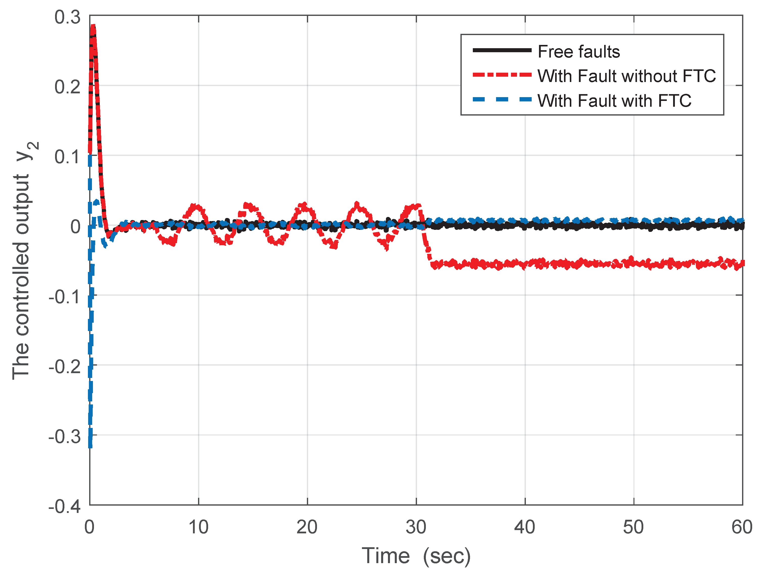
Figure 1 presents the actuator fault f a along with its estimated counterpart f ^ a . It can be seen that, despite the presence of disturbances, the proposed ASMO design achieves the estimation of the constant/time-varying actuator fault with satisfactory accuracy. The system’s output response y 2 under DOFFTC, including the actuator fault, is illustrated in Figure 2. It can be observed that the output y 2 without DOFFTC does not converge with the output of the fault-free model (i.e., without any fault). However, the output y 2 with DOFFTC reaches the output of the nominal model. Therefore, the proposed DOFFTC design achieves the performance under the actuator fault, and the stability of the closed-loop system is guaranteed.

6. Conclusions

This study confronts the intricate challenge of simultaneously addressing robust fault estimation (FE) and DOFFTC within T-S fuzzy systems. Our framework encompasses the incorporation of local nonlinear models, handling of unknown inputs, mitigation of measurement disturbances, and tackling of actuator faults. In response to these multifaceted issues, we introduce an ASMO, meticulously tailored to efficiently estimate actuator faults with both speed and precision, while also endowing the system with robustness against disturbances via H performance. Leveraging the fault estimation insights garnered, we craft a DOFFTC strategy, aimed at mitigating the adverse effects of actuator faults and ensuring stability for the closed-loop system. We present innovative design criteria expressed in the form of LMIs to guarantee the existence of the desired observer and controller. To demonstrate the efficacy of our approach, we provide an illustrative example involving an inverted pendulum mounted on a cart system.

Author Contributions

Conceptualization, S.D.; methodology, S.D.; validation, S.D. and O.N.; investigation, O.N.; visualization, O.N.; writing—original draft preparation, S.D.; writing—review and editing, O.N. All authors have read and agreed to the published version of the manuscript.

Funding

This research was funded by the Deanship of Scientific Research at Jouf University under grant no. (DSR-2021-02-0364).

Institutional Review Board Statement

Not applicable.

Informed Consent Statement

Not applicable.

Data Availability Statement

No data were used to support this study.

Conflicts of Interest

The authors declare no conflict of interest.

Abbreviations

The following abbreviations are used in this manuscript:
R n n-dimensional Euclidean space
R n × m set of real n × m matrices
A > 0 ( A < 0 )symmetric and positively (negatively) definite matrix A
A T transpose of matrix A
I n n-dimensional identity matrix
λ min ( A ) ( λ max ( A ) )minimum (maximum) eigenvalue of matrix A
. induced spectral norm or the Euclidean norm
*symmetric terms in a symmetric matrix
L 2 space of square integrable functions

Appendix A

Matrices used in example
A 1 = 0 1 0 0 g 4 l 3 m l a 0 0 b a 4 l 3 m l a 0 0 0 1 m g a 4 3 m a 0 0 b a 4 3 m a , B 1 = F 1 = 0 a 4 l 3 m l a 0 4 a 3 4 3 m a , N 1 = 0 g 4 l 3 m l a 0 g 4 3 m a A 2 = 0 1 0 0 g 2 2 π 4 l 3 m l a 2 0 0 b a 2 2 4 l 3 m l a 2 0 0 0 1 m g a 2 π 4 3 m a 2 0 0 b a 4 3 m a 2 , B 2 = F 2 = 0 a 2 2 4 l 3 m l a 2 0 4 a 3 4 3 m a 2 , N 2 = 0 g 4 l 3 m l a 2 0 g 4 3 m a 2 E = 0 0.1 0 0.1 , C = 1 0 0 0 0 0 1 0 0 0 1 1 , D = 0.1 0.1 0.1

References

  1. Takagi, T.; Sugeno, M. Fuzzy identification of systems and its applications to modeling and control. IEEE Trans. Syst. Man Cybern. Part B-Cybern. 1985, 15, 116–132. [Google Scholar] [CrossRef]
  2. Teixeira, M.C.M.; Zak, S.H. Stabilizing controller design for uncertain nonlinear systems using fuzzy models. IEEE Trans. Fuzzy Syst. 1999, 7, 133–142. [Google Scholar] [CrossRef]
  3. Tanaka, K.; Wang, H. Fuzzy Control Systems Design and Analysis: A Linear Matrix Inequality Approach; Wiley: Hoboken, NJ, USA, 2001. [Google Scholar]
  4. Feng, G. A survey on analysis and design of model-based fuzzy control systems. IEEE Trans. Fuzzy Syst. 2006, 14, 676–697. [Google Scholar] [CrossRef]
  5. Chang, X.; Yang, G.H. Relaxed stabilization conditions for continuous-time Takagi-Sugeno fuzzy systems. Inf. Sci. 2010, 180, 3273–3287. [Google Scholar] [CrossRef]
  6. Zhang, K.; Jiang, B.; Staroswiecki, M. Dynamic output feedback fault tolerant controller design for Takagi-Sugeno fuzzy systems with actuator faults. IEEE Trans. Fuzzy Syst. 2010, 18, 194–201. [Google Scholar] [CrossRef]
  7. Zhao, X.; Zhang, L.; Shi, P.; Karimi, H.R. Novel stability criteria for T-S fuzzy systems. IEEE Trans. Fuzzy Syst. 2014, 22, 313–323. [Google Scholar] [CrossRef]
  8. Li, H.; You, F.; Wang, F.; Guan, S. Robust fast adaptive fault estimation and tolerant control for T-S fuzzy systems with interval time-varying delay. Int. J. Syst. Sci. 2017, 48, 1708–1730. [Google Scholar] [CrossRef]
  9. Shahnazi, R.; Zhao, Q. Adaptive fuzzy descriptor sliding mode observer-based sensor fault estimation For uncertain nonlinear systems. Asian J. Control 2016, 18, 1478–1488. [Google Scholar] [CrossRef]
  10. Han, J.; Zhang, H.; Wang, Y.; Liu, X. Robust fault estimation and accommodation for a class of T–S fuzzy systems with local nonlinear models. Circuits Syst. Signal Process. 2016, 35, 3506–3530. [Google Scholar] [CrossRef]
  11. Dong, J.; Hou, J. Output feedback fault-tolerant control by a set-theoretic description of T–S fuzzy systems. Appl. Math. Comput. 2017, 301, 117–134. [Google Scholar] [CrossRef]
  12. Kharrat, D.; Gassara, H.; Hajjaji, A.E.; Chaabane, M. Adaptive observer and fault tolerant control for Takagi-Sugeno descriptor nonlinear systems with sensor and actuator faults. Int. J. Control Autom. Syst. 2018, 16, 972–982. [Google Scholar] [CrossRef]
  13. Yan, J.J.; Yang, G.H.; Li, X.J. Adaptive observer-based fault-tolerant tracking control for T–S fuzzy systems with mismatched faults. IEEE Trans. Fuzzy Syst. 2020, 28, 134–147. [Google Scholar] [CrossRef]
  14. Makni, S.; Bouattour, M.; Hajjaji, A.; Chaabane, M. Robust fault estimation and fault-tolerant tracking control for uncertain Takagi–Sugeno fuzzy systems: Application to single link manipulator. Int. J. Adapt. Control Signal Process. 2021, 35, 846–876. [Google Scholar] [CrossRef]
  15. Li, Y.; Xu, W.; Chang, L. Fuzzy model based fault estimation and fault tolerant control for flexible spacecraft with unmeasurable vibration modes. IET Cont. Theory Appl. 2022, 17, 19–38. [Google Scholar] [CrossRef]
  16. Dhahri, S.; Hmida, F.B.; Sellami, A. Robust H sliding mode observer design for fault estimation in a class of uncertain nonlinear systems with LMI optimization approach. Int. J. Control Autom. Syst. 2012, 10, 1032–1041. [Google Scholar] [CrossRef]
  17. Shaker, M.S.; Patton, R.J. Active sensor fault tolerant output feedback tracking control for wind turbine systems via T–S model. Eng. Appl. Artif. Intell. 2014, 34, 1–12. [Google Scholar] [CrossRef]
  18. Brahim, A.B.; Dhahri, S.; Hmida, F.B.; Sellami, A. Adaptive sliding mode fault tolerant control design for uncertain nonlinear systems with multiplicative faults: Takagi–Sugeno fuzzy approach. Proc. Inst. Mech. Eng. Part I J. Syst. Control Eng. 2019, 234, 147–159. [Google Scholar] [CrossRef]
  19. Brahim, A.B.; Dhahri, S.; Hmida, F.B.; Sellami, A. H Sliding mode observer for Takagi-Sugeno nonlinear systems with simultaneous actuator and sensor faults. Int. J. Appl. Math. Comput. Sci. 2015, 25, 547–559. [Google Scholar] [CrossRef]
  20. Feng, X.; Wang, Y. Fault estimation based on sliding mode observer for Takagi–Sugeno fuzzy systems with digital communication constraints. J. Frankl. Inst. 2020, 357, 569–588. [Google Scholar] [CrossRef]
  21. Li, S.; Wang, H.; Aitouche, A.; Christov, N. Sliding mode observer design for fault and disturbance estimation using Takagi–Sugeno model. Eur. J. Control 2018, 44, 114–122. [Google Scholar] [CrossRef]
  22. Zhang, K.; Jiang, B.; Cocquempot, V. Fuzzy unknown input observer-based robust fault estimation design for discrete-time fuzzy systems. Signal Process. 2016, 128, 40–47. [Google Scholar] [CrossRef]
  23. Hadi, A.S.; Shaker, M.S. A new estimation/decoupling approach for robust observer-based fault reconstruction in nonlinear systems affected by simultaneous time varying actuator and sensor faults. J. Frankl. Inst. 2020, 357, 8956–8979. [Google Scholar] [CrossRef]
  24. Emanoel, R.Q.; Chaves, J.; André, F.O.; Dantas, A.; Maitelli, A.L. Unknown input observer-based actuator and sensor fault estimation technique for uncertain discrete time Takagi-Sugeno systems. Int. J. Control Autom. Syst. 2021, 19, 2444–2454. [Google Scholar]
  25. Sun, S.; Zhang, H.; Wang, Y.; Cai, Y. Dynamic output feedback-based fault-tolerant control design for T-S fuzzy systems with model uncertainties. ISA Trans. 2018, 81, 32–45. [Google Scholar] [CrossRef] [PubMed]
  26. Cheridi, D.E.; Mansouri, N. Robust H fault-tolerant control for discrete-time nonlinear system with actuator faults and time-varying delays using nonlinear T–S fuzzy models. Circuits Syst. Signal Process. 2020, 39, 175–198. [Google Scholar] [CrossRef]
  27. Zhang, H.; Sun, S.; Liu, C.; Zhang, K. A novel approach to observer-based fault estimation and fault-tolerant controller design for T-S fuzzy systems with multiple time delays. IEEE Trans. Fuzzy Syst. 2019, 28, 1679–1693. [Google Scholar] [CrossRef]
  28. Dhahri, S.; Alaia, E.B.; Hmida, F.B.; Sellami, A. H fault estimation and fault-tolerant control for T-S fuzzy fystems with actuator and sensor faults using sliding mode observer. Math. Probl. Eng. 2022, 2022, 3647171. [Google Scholar] [CrossRef]
  29. Taniguchi, T.; Tanaka, K.; Ohtake, H.; Wang, H.O. Model construction, rule reduction, and robust compensation for generalized form of Takagi-Sugeno fuzzy systems. IEEE Trans. Fuzzy Syst. 2001, 9, 525–538. [Google Scholar] [CrossRef]
  30. Dong, J.X.; Wang, Y.Y.; Yang, G.H. Control synthesis of continuous-time T–S fuzzy systems with local nonlinear models. IEEE Trans. Syst. Man Cybern. Part B Cybern. 2009, 39, 45–58. [Google Scholar]
  31. Moodi, H.; Farrokhi, M. Robust observer-based controller design for Takagi–Sugeno systems with nonlinear consequent parts. Fuzzy Sets Syst. 2015, 273, 141–154. [Google Scholar] [CrossRef]
  32. Wang, H.M.; Ye, D.; Yang, G.H. Actuator fault diagnosis for uncertain T-S fuzzy systems with local nonlinear models. Nonlinear Dyn. 2014, 76, 1977–1988. [Google Scholar] [CrossRef]
  33. Moodi, H.; Farrokhi, M. On observer-based controller design for Takagi Sugeno systems with unmeasurable premise variables. ISA Trans. 2014, 53, 305–316. [Google Scholar] [CrossRef]
  34. Jiang, B.; Wang, J.L.; Soh, Y.C. An adaptive technique for robust diagnosis of faults with independent effects on system outputs. Int. J. Control 2002, 75, 792–802. [Google Scholar] [CrossRef]
  35. Tuan, H.D.; Apkarian, P.; Narikiyo, T.; Yamamoto, Y. Parameterized linear matrix inequality techniques in fuzzy control system design. IEEE Trans. Fuzzy Syst. 2001, 9, 324–332. [Google Scholar] [CrossRef]
  36. Chilali, M.; Gahinet, P. H design with pole placement constraints: An LMI approach. IEEE Trans. Autom. Control 1996, 41, 358–367. [Google Scholar] [CrossRef]
  37. Corless, M.; Tu, T. State and input estimation for a class of uncertain systems. Automatica 1998, 34, 757–764. [Google Scholar] [CrossRef]
  38. Raoufi, R.; Marquez, H.J.; Zinober, A.S.I. H sliding mode observers for uncertain nonlinear Lipschitz systems with fault estimation synthesis. Int. J. Robust. Nonlinear Control 2010, 20, 1785–1801. [Google Scholar] [CrossRef]
  39. Utkin, V.I. Sliding Modes in Control Optimization; Springer: Berlin, Germany, 1992. [Google Scholar]
  40. Gao, Z.; Antsaklis, P.J. Reconfigurable control system design via perfect model following. Int. J. Control 1992, 56, 783–798. [Google Scholar] [CrossRef]
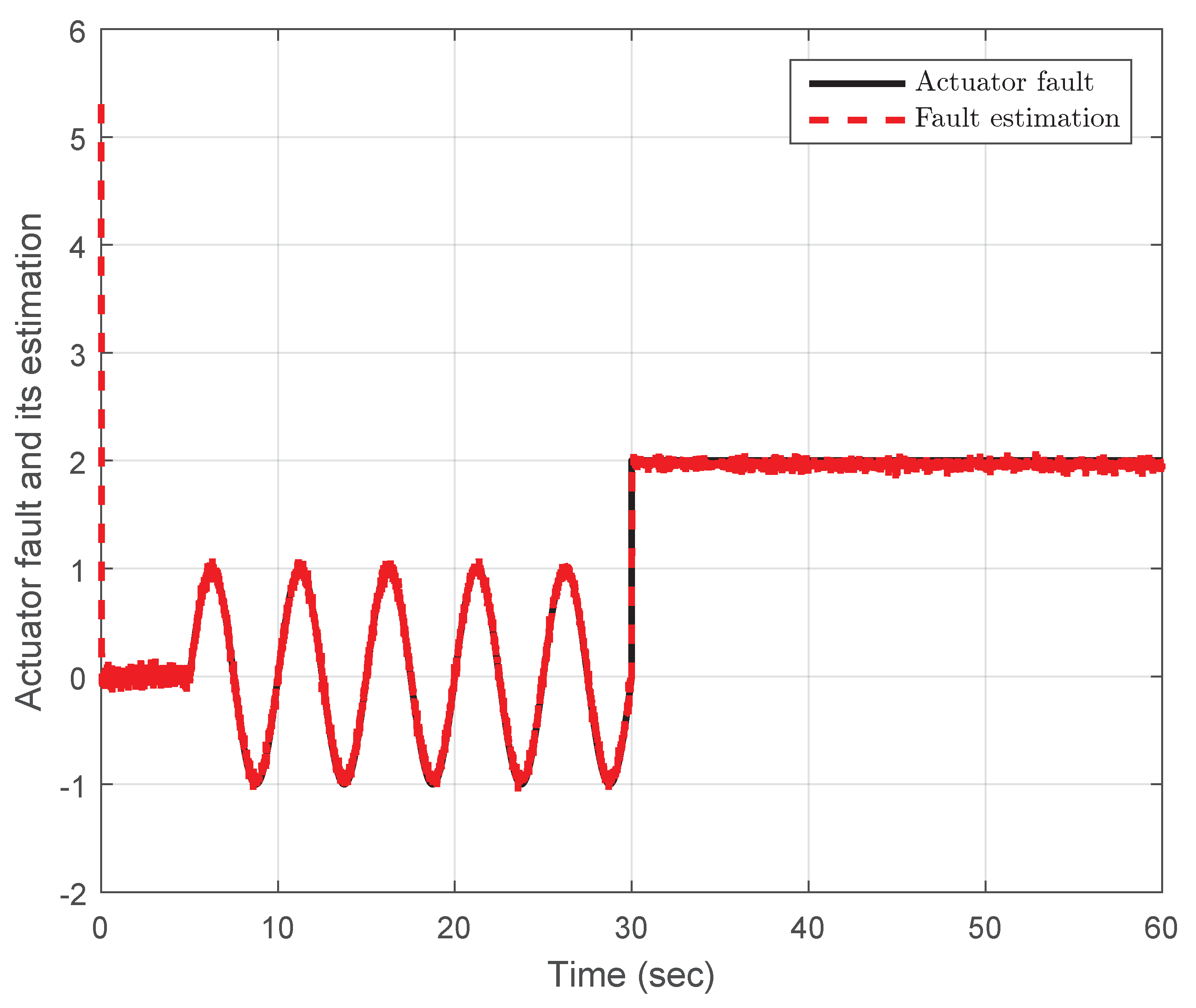
Figure 1. Actuator fault f a and its estimation.
Symmetry 15 01894 g001
Figure 2. Output response y 2 with and without FTC.
Symmetry 15 01894 g002
Disclaimer/Publisher’s Note: The statements, opinions and data contained in all publications are solely those of the individual author(s) and contributor(s) and not of MDPI and/or the editor(s). MDPI and/or the editor(s) disclaim responsibility for any injury to people or property resulting from any ideas, methods, instructions or products referred to in the content.