Article

Parameter Identification in Metabolic Reaction Networks by Means of Multiple Steady-State Measurements

1
Institute for Systems Analysis and Computer Science ‘A. Ruberti’ (IASI-CNR), Via dei Taurini 19, 00185 Rome, Italy
2
SYSBIO—Centre of Systems Biology, Piazza della Scienza 2, 20126 Milan, Italy
3
Center of Excellence for Research DEWS, University of L’Aquila, Via Vetoio 1, 67100 L’Aquila, Italy
4
Faculty of Engineering, Campus Biomedico University of Rome, Via Álvaro del Portillo 21, 00128 Rome, Italy
5
Department of Biotechnology and Biosciences, University of Milano-Bicocca, Piazza della Scienza 2, 20126 Milan, Italy
*
Authors to whom correspondence should be addressed.
Symmetry 2023, 15(2), 368; https://doi.org/10.3390/sym15020368
Submission received: 24 December 2022 / Revised: 22 January 2023 / Accepted: 25 January 2023 / Published: 30 January 2023
(This article belongs to the Section Life Sciences)

Abstract

:
In this work, we investigate some theoretical aspects related to the estimation approach proposed by Liebermeister and Klipp, 2006, in which general rate laws, derived from standardized enzymatic mechanisms, are exploited to kinetically describe the fluxes of a metabolic reaction network, and multiple metabolic steady-state measurements are exploited to estimate the unknown kinetic parameters. Further mathematical details are deeply investigated, and necessary conditions on the amount of information required to solve the identification problem are given. Moreover, theoretical results for the parameter identifiability are provided, and symmetrical and modular properties of the proposed approach are highlighted when the global identification problem is decoupled into smaller and simpler identification problems related to the single reactions of the network. Among the advantages of the proposed innovative approach are (i) non-restrictive conditions to guarantee the solvability of the parameter estimation problem, (ii) the unburden of the usual computational complexity for such identification problems, and (iii) the ease of obtaining the required number of measurements, which are actually steady-state data, experimentally easier to obtain with respect to the time-dependent ones. A simple example concludes the paper, highlighting the mentioned advantages of the method and the implementation of the related theoretical result.

1. Introduction

Mathematical models definitely increase the understanding of complex biological functions and how they arise from the interactions of large numbers of gene products and metabolic molecules. Metabolic mathematical models, both large-scale ones or much simpler models focused on constituent pathways, allow for comprehensively investigating the mechanisms underlying given phenotypes and making hypotheses testable in the laboratory.
Different modeling frameworks are used to predict the behavior of the cell metabolism, from constraint-based to mechanistic kinetic models [1]. The first ones allow us to give a structural analysis of the metabolic network and provide a steady-state picture of its working state, exploiting only the stoichiometry information. These methods substantially increase the knowledge of the possible network operation states of a given organism (see e.g., [2,3]) and have the potential to bring substantial advantages in biotechnological applications. However, they do not explain how metabolic steady-states are attained, as the necessary kinetic information is missing. Conversely, mechanistic kinetic models take explicitly into account the molecular details of reactions describing the formation/rupture of chemical bonds and the formation/release of new compounds. Therefore, they introduce the explicit dependency of the reaction fluxes on metabolite and enzyme concentrations. However, reaction fluxes also depend on stoichiometry and kinetic constants, which are physically meaningful quantities related to the specific mechanism under investigation. Many kinetic models are given in the scientific literature; examples of the ones developed for the Saccharomyces cerevisiae can be found in BioModels Database [4].
Building kinetic mathematical models of metabolism is actually a very complex task as such a cell function is governed by many chemical transformations, characterized by a variety of different molecular mechanisms, often not completely known. Moreover, the reconstruction of a metabolic network of a given organism requires also the availability of a huge number of experimental observations and quantitative data. The resulting network is usually very complicated and tangled, making any kind of mathematical analysis very difficult, as for instance the evaluation of the kinetic parameters of the chemical transitions. Such an identification task usually consists in estimating a huge number of unknown parameters from scarce experimental data, often difficult to be measured. However, the parameter estimation can be greatly simplified if a suitable modeling framework is adopted, aiming at introducing symmetries between the chemical reactions and at making the whole network modular. Indeed, the estimation approach here investigated (originally proposed by Liebermeister and Klipp [5,6]) assumes the form of a general molecular mechanism for describing the mechanistic details of all the reactions, hence introducing a symmetric scheme within the metabolic network that makes the network structure actually modular. Such modularity (together with the knowledge of steady-state fluxes) permits the decoupling of the global identification problem into smaller, simpler, and symmetric subproblems. This is the main advantage of the proposed approach, introducing symmetries and modularities in the network structure that allows for reducing the complexity of the identification task.
Kinetic parameters are crucial for model prediction, as their values strongly influence the state behavior. Therefore, the knowledge of the “true” value of the kinetic parameters, or at least inferring a “realistic” value (i.e., “close” to the real one) for them, is mandatory to reliably simulate the metabolic dynamics. However, such an important identification problem becomes harder for large-scale metabolic networks, as for instance [7,8,9]. In these cases, the accurate identification of all the kinetic parameters is actually unrealistic, unless an extraordinary measurement effort (unavoidably implying a huge economic cost) is performed. Some authors proposed innovative methods to overcome this typical lack of kinetic information, as the building of ensemble models, which are families of models (equivalent in terms of the steady state finally reached) allowing to examine phenotype changes due to enzyme level perturbations [10]. Another shortcoming of building metabolic models is that the mechanistic details of many enzymatic reactions are unknown and their determination requires a remarkable experimental effort. Therefore, some authors suggest representing unknown kinetic laws by exploiting standard rate mechanisms, such as mass-action or generalized Michaelis–Menten (MM) kinetics [11,12], or the convenience rate law proposed by [5].
The identification problem of the unknown kinetic parameters, both coming from true known mechanisms or from standardized ones, is carried out by exploiting some experimental information on the system. Direct measurements of the kinetic parameters are not frequently available, since the related physical quantities are usually not easily measurable. The identification method usually adopted to estimate such parameters is the classical approach exploiting time-course measurements of the metabolite concentrations and a fitting procedure minimizing the residuals between the model prediction and the experimental time measurements. However, the main limitation of such an approach is the difficulty in obtaining a huge number of temporal measurements, particularly placed in the “right” time instants of the state evolution (to maximize the dynamical information content). Unfortunately, only a few time samples can usually be measured over time; this is due to practical restrictions of the available devices and of the measurement process. Moreover, requiring high numbers of time samples unavoidably implies high experiment costs.
Another drawback of time-dependent identification is related to the dependency of the state’s dynamical behavior on its initial value. Therefore, to obtain a reliable estimation of the kinetic parameters, a concomitant estimation of kinetic parameters and initial conditions should be carried out, increasing the number of unknowns of the estimation problem (as well as the number of required experimental data).
An alternative approach for the estimation of the kinetic parameters has been proposed by Liebermeister and Klipp, 2006. The approach proposed in the seminal paper [6] consists in identifying kinetic parameters exploiting steady-state measurements of metabolite concentrations related to different external conditions, like enzyme and substrate concentrations. The knowledge of multiple steady-states is a necessary condition required by this approach as the number of kinetic parameters is usually much larger than the number of internal metabolites of the network. They also provide an iterative procedure to integrate knowledge into the system and to on-line update, the values of the model parameters denoted as the parameter balancing technique [11,12].
In the present paper, we go in-depth into the mathematical details of an approach consisting of merely multiple steady-state measurements, providing conditions on the amount of information (i.e., the number of steady states) required to solve the identification problem and giving theoretical results for the parameter identifiability. The mathematical models exploited to deal with general metabolic networks and the proposed kinetic parameter identification procedure are described in Section 2 and Section 3, respectively. The particular structure of the steady-state identification problem allows us to give an important theoretical result regarding the local identifiability of the unknown parameters, given in Section 4. In addition to the formalization of the identification procedure that exploits stationary (rather than transient) measurements, the identifiability result of Section 4 is the novelty of the manuscript.
Below we highlight the main advantages carried out by the proposed alternative method, which overcomes the limitations of the classical identification procedures.
First of all, the alternative estimation reduces to solve a nonlinear system which reveals to be actually polynomial w.r.t. the unknown parameters, provided that the kinetic laws are chosen among the standard widespread kinetic mechanisms, as mass-action, or Michaelis-Menten, or the convenience rate law proposed by [5]. Conversely, the classical time-dependent identification leads to the solution of a nonlinear system which is usually non-polynomial.
The alternative approach requires a lower number of measurements than the classical one, and the required measurements are metabolite concentrations at steady state, which are easier to be obtained w.r.t. time-course measurements.
The proposed steady-state estimation approach becomes easier when both metabolite concentrations and fluxes (usually determined by constraint-based techniques, [13]) are known, even though this complete knowledge concerns only a subsystem of the considered network. Indeed, in this case, we can split the identification into two steps: (1) identification of the subsystem parameters, exploiting both fluxes and metabolite concentrations; (2) identification of the kinetic parameters of the whole network, using only the available concentration measurements and the subsystem parameter values estimated in the previous step, entering this second estimation round as a priori knowledge. The complexity of the identification is highly reduced in this way. In particular, in step (1) the system complexity is reduced by decoupling the problem into smaller and simpler subproblems related to the single reactions. This decomposition highlights modular and symmetrical properties of the algebraic system, which are extremely relevant as they reduce the computational burden of the identification task, and allow us to further reduce the number of required steady-state measurements (which is a non-negligible aspect, especially for large-scale networks). Moreover, in this case, the local result given in Section 4 becomes global for many simple kinetic mechanisms, as in the case of mass-action or one-to-one bidirectional Michaelis–Menten.
Finally, the methodology is applied to a simple metabolic network, highlighting the aforementioned advantages with respect to standard methods exploiting time-course measurements.

2. Mathematical Models of Metabolic Networks

Let us define the following metabolic reaction network:
i = 1 n α i , j A i j i = 1 n β i , j A i , j = 1 , 2 , , r ,
where A i , i = 1 , 2 , , n , are n metabolites affected by r chemical conversions j = 1 , 2 , , r , while α i , j and β i , j are the stoichiometric coefficients describing the number of A i molecules consumed and produced by the j-th reaction, respectively; A i can be classified w.r.t. the reaction j as: (i) reactant, when α i , j > 0 , β i , j = 0 , (ii) product, when α i , j = 0 , β i , j > 0 , (iii) both reactant and product, when α i , j , β i , j > 0 , (iv) not affected, when α i , j , β i , j = 0 . Let us also denote by x the ( n × 1 ) vector of the metabolite concentrations [ A i ] ( x i = [ A i ] , i = 1 , , n ) and by ν the ( r × 1 ) vector of the reaction fluxes ν j , j = 1 , , r . Each flux ν j provides the net amount of metabolites converted into products by reaction j per unit time and per unit mass. The dynamic equations of the metabolite concentrations can be written as
d x d t = N ν ,
where N is the ( n × r ) stoichiometry matrix collecting all the net stoichiometric coefficients s i , j = β i , j α i , j , i = 1 , 2 , , n , j = 1 , 2 , , r .
The model Equation (2) can be used to perform several analyses in metabolic networks. First of all, the network steady state can be analyzed by means of constraint-based techniques which are able to infer the stationary flux distribution throughout all the network reactions under given external conditions and, consequently, to efficiently highlight emerging phenotypes [13]. Such methods only depend on the algebraic system of linear equations
N ν = 0 ,
coming from the steady-state condition d x / d t = 0 , which constrains the stationary values of the r fluxes of the biochemical network. The determination of the steady-state flux distribution in metabolic networks, i.e., the identification of a particular flux vector ν solving system (3), has a deep interest in biology since the majority of homeostatic states in cell metabolism can be approximately described by the steady-state condition d x / d t = 0 . Indeed, since metabolism has a much faster time scale (minutes) than other processes (hours, like regulatory processes, cell division events, etc.), it is reasonable to assume that, when the external conditions are kept fixed, metabolism has already reached a quasi-steady-state condition while the other cell processes are still running.
Despite the potential of constraint-based methods and the wide information arising from the steady state, in many applications it is mandatory to provide a temporal description of the metabolite concentrations, like for instance when the external conditions are rapidly changing and the transient behavior of metabolites gains more interest. In this case, we need to establish specific kinetic laws between the reaction fluxes and the metabolite concentrations, ν = ν ( x ) , to transform system (2) into an ODE system in terms of the state vector x:
d x d t = N ν ( x ) .
The mathematical expression of each kinetic law ν j ( x ) , j = 1 , , r , depends at least on the substrate concentrations of reaction j, as in the simplified case of unidirectional reaction, or, more in general, on both substrate and product concentrations when the reaction is more realistically modeled as bidirectional. Moreover, the mathematical expression of the law ν j ( x ) also depends on the biochemical mechanism used to represent the metabolic conversion of reactants into products through reaction j. However, such kinetic laws depend also on unknown constant parameters, i.e., on physically meaningful quantities that characterize the assumed biochemical mechanism. The more complex and detailed the chosen mechanism, the higher the number of unknown kinetic parameters, as well as the higher the uncertainty on their values.
The most common kinetic mechanisms used to describe biochemical reactions are (i) the mass action, (ii) the Michaelis–Menten, and (iii) the convenience kinetics [5]. The mass action mechanism provides a kinetic law for a reaction flux that is proportional to the product of the substrate concentrations (raised to the power of their stoichiometric coefficients). Therefore, denoting by k j the reaction rate constant (a proportionality coefficient providing the speed of the reaction bonding), by the superscripts f and b the quantities related to the forward and, respectively, backward reaction, and by F j and B j the sets of metabolite indexes identifying the substrates of the forward and, respectively, the backward flux of reaction j, the mass action law is given by
ν j = ν j f = k j f i F j [ A i ] α i , j , and ν j = ν j f ν j b = k j f i F j [ A i ] α i , j k j b i B j [ A i ] β i , j ,
describing unidirectional and, respectively, bidirectional reactions [14].
The Michaelis–Menten mechanism is slightly more complex than the mass action law and it is usually adopted to describe enzymatic reactions. Such a kinetic law has been originally formulated for unidirectional reactions and it assumes a double-step mechanism for the product formation: (i) the first one which is fast and produces the enzyme-substrate complex; (ii) the second one, which is slower than the first (and then rate limiting), converting the complex into product [14]. Under suitable simplifying assumptions, the resulting kinetic law for a one-to-one, single-substrate, single-product unidirectional reaction is given by
ν j = ν j f = k j f [ S j ] K j f 1 + [ S j ] K j f ,
where [ S j ] is the concentration of the substrate of reaction j while K j f is the related Michaelis–Menten constant, which gives the substrate concentration at which the flux size is half of the maximal achievable value, i.e., k j f / 2 [14]. The former mechanism can be easily extended for the case of bidirectional reactions as
ν j = ν j f ν j b = k j f [ S j ] K j f k j b [ P j ] K j b 1 + [ S j ] K j f + [ P j ] K j b ,
where [ S j ] , [ P j ] are the metabolite concentrations feeding the forward and, respectively, the backward flux of reaction j, while K j f , K j b are the related Michaelis–Menten constants [14]. Note that, for both laws (6) and (7), the concentrations of the enzymes that catalyze the reaction deeply influence the size of the constants k j f , k j b . In particular, assuming that the same enzyme is involved in the catalysis of the forward and backward reaction, it is k j f = [ E j ] h j f , k j b = [ E j ] h j b , where [ E j ] is the concentration of the enzyme E j catalyzing reaction j and h j f , h j b are suitable rate constants related to the forward and backward fluxes. Note that accounting for the enzyme expression levels in the kinetic model is mandatory in some applications, as the intriguing Enzyme Cost Minimization (ECM) approach proposed by Noor et al. [15].
The convenience rate law generalizes the MM law for multi-substrate, multi-product reactions with stoichiometry higher than one, and it is given by
ν j = [ E j ] h j f i F j [ A i ] K i , j f α i , j 1 + i F j l = 0 α i , j [ A i ] K i , j f l , and ν j = [ E j ] h j f i F j [ A i ] K i , j f α i , j h j b i B j [ A i ] K i , j b β i , j i F j l = 0 α i , j [ A i ] K i , j f l + i B j l = 0 β i , j [ A i ] K i , j b l 1 ,
respectively related to unidirectional and bidirectional mechanisms. See the paper [5] for more details on the mathematical derivation of the convenience rate law. Note that, similarly to Equations (6) and (7), the rate laws given by Equations (8) show a realistic saturation behavior with respect to the metabolite concentrations, which is not modeled by the mass-action law. However, this important modeling aspect produces an increase in the number of unknown parameters for each reaction, moving from the minimum of two parameters, in the case of mass-action assumption, to four, in the case of single-substrate single-product convenience rate law, or more unknown parameters (in precisely two plus the number of metabolites involved in the reaction), in the case of multi-substrate multi-product convenience rate law. This means that we need to assign values from 2 r to 2 r + j = 1 r n j unknown parameters, where n j represents the number of metabolites involved in reaction j, to characterize the dynamic behavior of the network under investigation.
We finally note that all the kinetic laws considered above can be extended by taking some regulation mechanisms into account. In particular, we can consider the activation or the inhibition of some reaction rates by means of the amount of given network metabolites. This biochemical control aspect can be modeled by simply adding a factor multiplying the kinetic rate law of the regulated reaction (see [14]), that is
φ j A = [ A i ] [ A i ] + K A , φ j I = K I [ A i ] + K I ,
respectively for the activation and the inhibition of reaction j by means of metabolite i. Obviously, the considered regulation mechanism adds a further unknown parameter to be estimated for each regulation mechanism introduced into the model.
The following Table 1 resumes the number of unknown parameters with respect to the modeling choice at hand.

3. Kinetic Parameter Identification in Metabolic Networks

The main problem of the kinetic biochemical models like system (4) is the identification of the model parameters, that is the evaluation of “reasonable” values for these unknown quantities. The number of kinetic parameters rapidly grows as the “realism” (and then the complexity) of the reaction mechanism increases, while the number of experimental data available for parameter identification is usually very low.
Independently of the kinetic detail chosen to represent the reaction mechanism, the kinetic model (4) can be rewritten making explicit the dependence of ν on kinetic parameters and on other fixed metabolic quantities, such as enzyme and external metabolite concentrations possibly tunable by the experimenter. Therefore, denoting by θ R p and u R m the vectors of the p unknown kinetic parameters and, respectively, of the m fixed metabolic quantities (enzymes and external metabolites), we get:
d x d t = N ν ( x , u , θ ) = f ( x , u , θ ) ,
where f is the vector field representing the state dynamic of x. We stress that the model formulation (10) assumes that the only metabolites changing over time are the ones collected by x (internal metabolites), while the ones collected by u are tunable from the outside of the network and fixed over time. Conversely, the kinetic parameter vector θ is assumed to be constant for a given metabolic network and not modifiable by the experimenter.
The identification problem of the unknown kinetic parameter vector θ can be accomplished if experimental data on the metabolic system are acquired. For instance, if direct measurements of the physical quantities represented by the kinetic parameters of θ were available, a least square estimation problem could be straightforwardly solved. However, direct measurements of θ are not frequent since the related physical quantities are usually not easily measurable.
The classical identification approach used to estimate the parameters of a dynamical system is the one exploiting time-course measurements of the state x. If we had a suitable number of time measurements of the metabolite concentrations (entries of x), we could in principle estimate the kinetic parameter vector θ by exploiting a fitting procedure based on the minimization of the residuals between the model prediction
x ( t ) = ϕ ( t ; x 0 , u , θ ) = x 0 + 0 t f ( x ( τ ) , u , θ ) d τ ,
and the experimental measurements of x. However, there are several shortcomings, both experimental and computational, of such a kind of approach applied to metabolic networks. The main ones are the experimental limitations in obtaining a huge number of time measurements in the right time instants. Indeed, as explained above, metabolism is a fast process, characterized by short transient periods. So, to obtain measurements with high dynamical information content, we need to intensely sample the metabolite time course before the steady state. This means “many and close” time measures. Unfortunately, only few and far time samples can usually be measured over time because of practical restrictions of the available devices and the measurement process, which unavoidably limits the frequency of measurement. Moreover, the number of time samples significantly affects the cost of the experiment. Then, such experimental limitations lead to few time samples, usually close to the steady state.
Moreover, such a time-dependent identification approach has also a computational drawback due to the fact that the dynamical behavior of the model prediction (11) depends both on the kinetic parameter vector θ and on the state initial condition x 0 . So to make the estimation of the kinetic parameters independent of the initial state, a concomitant estimation of parameters and initial conditions should be carried out, so increasing the number of unknowns of the estimation problem and, consequently, the number of experimental measurements required to reliably identify them. More specifically, in the absence of measurement noise, denoting by x ˜ l the ideal measure of the state vector x at the measurement time t ˜ l , the classical identification problem is accomplished by solving the nonlinear non-polynomial system
ϕ ( t ˜ l ; x 0 , u , θ ) = x ˜ l , l = 1 , 2 , , L ,
w.r.t. the unknown ( x 0 , θ ) , for a given fixed value of u. Note that the number of the equations of system (12) must be larger than the number of unknowns to obtain a finite number of solutions, that is n L n + p .
As an alternative way to estimate the kinetic parameters of the dynamical system (10), in the spirit of [6], we propose an approach that exploits the knowledge of multiple metabolic steady states given by different values of the external settings u. Let us assume to fix M different fixed settings for u, denoted by u ( l ) , l = 1 , 2 , , M , and to measure the related steady state of x for each one of them. Let us denote the steady state of x using a bar over the variable and a bracketed number referring to the corresponding external setting. So x ¯ ( l ) represents the steady state of x related to the external setting u ( l ) . The alternative identification problem consists in solving the following nonlinear system
f ( x ¯ ( l ) , u ( l ) , θ ) = N ν ( x ¯ ( l ) , u ( l ) , θ ) = 0 , l = 1 , 2 , , M ,
w.r.t. θ . Note that the knowledge of a single metabolic steady state x ¯ ( l ) related to a specific value u ( l ) would be insufficient to determine all the kinetic parameters since the information content of one steady state is not enough to completely capture the dynamical aspects of the ODE systems. In fact, the number of kinetic parameters usually outnumbers the number of internal metabolites, i.e., p > n , and then at least aggregate parameter ensembles could be inferred from the n steady-state conditions coming from (13) with M = 1 . However, if the number of known metabolic states M were such that n M p , the identification problem could be performed.
Such an alternative approach provides several advantages, overcoming some limitations of the classical method:
  • the nonlinear system (13) reduces to a polynomial system with respect to the kinetic parameters, for any chosen kinetic mechanism among the standard ones (mass-action, MM, convenience, etc.). In fact, system (13) is a linear combination of reaction rates of the kinds given by Equations (5)–(8); when such rate laws are rational, each balance equation of system (13) can be transformed into a polynomial multiplying by the denominators of the related rate laws, which are always strictly positive (as they are given by 1 plus non-negative terms). Conversely, the nonlinear system (12) is usually non-polynomial;
  • system (13) requires a lower number of measurements than system (12) to be solved, allowing to spare a number of experimental measures equal to the state dimension n; this advantage increases as the network dimension increases;
  • the required measurements are metabolite concentrations at steady-state, which are easier to be obtained w.r.t. time-course measurements;
  • the computational burden of solving system (13) is lower than the one required to solve system (12), as a direct consequence of points 1 and 2: system (13) is a polynomial system with a lower number of equations w.r.t. system (12).
The alternative estimation approach can be further simplified when the distribution of the network fluxes ν is known. The determination of ν for a given external setting u can be carried out by means of constraint-based techniques like the basic Metabolic Flux Analysis (MFA) [13], the Flux Balance Analysis (FBA) [16] and Carbon 13 Metabolic Flux Analysis (C-13 MFA) [17]. All these techniques are mixed experimental/theoretical approaches (with significant computational aspects) and allow to find particular vectors among the solutions of the algebraic linear system (3) w.r.t. the unknown ν . Since the more frequent condition in metabolic networks is r a n k ( N ) < n < r , system (3) is usually undetermined, meaning that the only r a n k ( N ) linearly independent equations are not sufficient to uniquely determine the r unknowns. This undetermined condition is overcome by the constraint-based techniques that allow to pick up specific flux vectors within the null space of N by adding further constraints to system (3), like flux measurements, as in MFA, or an heuristic function of the fluxes to be optimized, as in FBA, or measurements of isotopomer abundances of the internal metabolites (when the network is fed by a specific labeled 13C-nutrient), as in C-13 MFA. In summary, all these techniques allow us to determine the network flux distributions related to the M external settings, adding further knowledge about the metabolic network beyond the measured stationary values of the internal metabolites. Therefore, knowing the steady-state values of the internal metabolite vectors { x ¯ ( 1 ) , x ¯ ( 2 ) , , x ¯ ( M ) } and of the flux vectors { ν ¯ ( 1 ) , ν ¯ ( 2 ) , , ν ¯ ( M ) } related to the M external fixed settings { u ( 1 ) , u ( 2 ) , , u ( M ) } , the solution θ of the nonlinear polynomial system (13) can be equivalently obtained by solving the following reduced nonlinear polynomial system:
ν ( x ¯ ( l ) , u ( l ) , θ ) = ν ¯ ( l ) , l = 1 , 2 , , M .
Solving system (14) w.r.t. θ requires a number M of measured steady states that are definitely lower than that required to solve system (13) (and consequently much lower than system (12)). This reduction comes from the condition r M p , which is required to obtain a finite number of solutions, and from the fact that the reaction number is usually higher than the number of internal metabolites, r > n (the relation becomes stronger, i.e., r > > n , for large-scale networks). Note that, as for system (13), also the equations of system (14) can be converted into polynomials, by simply multiplying the rate laws (in one of the forms (5)–(8)) by the positive denominators.
Actually, the computational complexity of system (14) can be further reduced by observing that the r algebraic equations of system (14) for a given fixed l can be symmetrically decoupled, as the kinetic parameters of a given reaction do affect only the corresponding reaction rate. Therefore, by partitioning the parameter vector θ into r subvectors
θ = θ 1 θ 2 θ r ,
where θ j R p j , j = 1 , 2 , , r , and  j = 1 r p j = p , system (14) can be rewritten as
ν j ( x ¯ ( l ) , u ( l ) , θ j ) = ν ¯ j ( l ) , j = 1 , 2 , , r , l = 1 , 2 , , M .
Remark 1.
Note that even in the presence of multiple 13C tracers, large and complex networks cannot be completely resolved, since isotopomer measurements coming from 13C labeled tracer experiments are difficult and expensive to collect. Usually, these kinds of high informative measures concern only a limited number of network metabolites, especially when large-scale networks are considered. However, just to mention some numbers, the gas chromatography/mass spectrometry (GM-MS) technique is able to provide much redundant information on the network and can give more than fifty mass isotopomer measurements, which is an information content that allows to reliably estimate around twenty unknown reaction fluxes by means of C13-MFA [13]. Moreover, different from measurements acquired at different time points, stationary measurements do not require fast measurement devices (i.e., measurements devices with dynamics faster than the one under investigation), and may benefit from redundant measurements for the same feature. We finally remark that although the computational implementation of the C13-MFA technique is actually non-trivial, since it implies solving a high number of non-linear isotopomer balances and a non-linear least square regression problem, nowadays, we have many user-friendly software packages easily implementing the computation of 13C-MFA problems [18,19,20].
Remark 2.
Evaluating the fluxes of a given subsystem within the network under investigation, for instance using C13-MFA is certainly advantageous for the proposed alternative identification. Indeed, the identification can be split into two steps: (1) we firstly identify the kinetic parameters of the subnetwork characterized by complete knowledge, exploiting both fluxes and metabolite concentrations and solving the reduced algebraic Equation (16), for each reaction of the subnetwork; (2) then, we perform the identification of the remaining kinetic parameters by solving the algebraic Equation (13) related to the whole network, but using only the available metabolite concentrations and exploiting the kinetic parameters already estimated as a priori known. The complexity of the identification is highly reduced in this way. In particular, step (1) allows the decoupling of the identification problem of the subnetwork parameters into smaller and simpler subproblems related to the single reactions. This decomposition reduces the computational burden of the identification task and highlights the modular and symmetrical properties of the algebraic subsystem. Obviously, also step (2) simplifies, benefiting from the knowledge coming from step (1).

4. Parameters Identifiability Conditions

In this section we provide the main contribution of this work, giving identifiability conditions for the kinetic parameters of a metabolic network, like the one described by Equation (10). The identifiability results given in the following subsections generally provide a local condition, i.e., valid in a neighborhood of the true parameter vector, but in some simple cases, the condition becomes global. In the following arguments we will assume that the concentrations of metabolites and enzymes at steady state are known, and that there are “enough” metabolic measurements to compute some Jacobian matrices (the concept of minimal information content required for the Jacobian computation is clarified below). Two identification approaches are investigated, a general one characterized by a lower information content in which fluxes are unknown and a simplified one characterized by high information with flux availability.
For the sake of clarity, we retrieve here a classical result of differential calculus that is used in the results of the next subsections [21].
Theorem 1
(Inverse Function Theorem). Let Ω R n be an open set and let x 0 Ω . If  f : Ω R n is a continuous function with continuous derivative, and if the Jacobian matrix of f is non-singular at x 0 :
| J f ( x 0 ) | = f ( x ) x x 0 0
then there exists a neighbourhood of x 0 , U x 0 Ω , such that the restriction of f to U x 0 , f | U x 0 : U x 0 f ( U x 0 ) is invertible, with  g = f 1 continuous with continuous derivative on f ( U x 0 ) .

4.1. Unknown Fluxes

The theorem given in this subsection provides a theoretical result on the local identifiability of the unknown kinetic parameters, in a general identification scenario in which a low information content is available. In particular, we assume that the network flux distribution is completely unknown.
Let us first define an extended function collecting the dynamic function of the system evaluated at different steady states.
Definition 1
(ESS function). Consider a function f defined as in (10), where the parameter vector is s.t. θ R p . Given the M steady state values ( x ¯ ( l ) , u ¯ ( l ) ) , l = 1 , , M , let us define the functions f ( l ) ( θ ) = f ( x ¯ ( l ) , u ¯ ( l ) , θ ) , l = 1 , , M . When p is a multiple of n the Extended Steady State (ESS) function is defined as
F ( θ ) = f ( 1 ) ( θ ) f ( 2 ) ( θ ) f ( M ) ( θ ) , F : R p R n M
where the number of known steady states M must be chosen s.t. n M = p . Conversely, when p is not a multiple of n, the number M will be chosen s.t. n M > p and the ESS function will be a p-dimensional sub-vector of function (18), obtained by selecting only some rows for each entry f ( l ) ( θ ) (so that the final dimension is actually the desired p dimension).
Remark 3.
The continuous differentiability of F obviously depends on the type of kinetic law chosen for modeling the reaction rates. This property is certainly verified for the most common kinetic laws, as Mass Action, Michaelis–Menten, Hill functions, and Convenience Rate (as the admissible parameter values must be positive). More in general, the continuity of the derivatives of F w.r.t. θ must be checked.
Let us now give the following identification result.
Theorem 2
(Network Identification with Unknown Fluxes). Given the metabolic network described by (10) and an ESS function F ( θ ) of dimension p (obtained collecting M p steady-state measurements), if the following Jacobian matrix is non-singular
F ( θ ) θ θ * 0 ,
where θ * is the true value of the parameter vector θ, then there exists a neighbourhood of θ * , V θ * , such that the identification problem
θ ^ = arg min θ V θ * F ( θ ) 2
admits a unique solution that coincides with the true value of the system parameters θ ^ = θ * .
Proof. 
The proof of the Theorem directly comes from the application of the Inverse Function Theorem to the function F ( θ ) . The regularity hypotheses of F are guaranteed in Ω R p , which is actually the positive orthant of R p , for standard reaction rates, or an open subset to be suitably identified, for more specific reaction rates. If the Jacobian condition (19) holds, i.e., if the determinant of the Jacobian of F with respect to θ at the true value θ * Ω is non-singular, by means of Theorem 1 there exists V θ * Ω such that the restriction of F to V θ * : F | V θ * is invertible. Noticing that the image of F | V θ * contains 0, since F ( θ * ) = 0 and recalling that F | V θ * is invertible, it follows that there exists a unique value of θ such that the F | V θ * = 0 , and this value is actually θ * , thus, θ ^ = θ * . This implies that the minimization problem (20) admits a unique solution which is the true value of the parameters.    □
Remark 4.
In practice, when dealing with the minimization problem (20), a numerical procedure is used. Usually one would have to fix an initial condition for the minimization algorithm. What the theorem implies is that, given the other hypotheses, if the initial condition lays inside the open set V θ * , then the minimum will be unique and it will coincide with the true value of the parameter vector.

4.2. Known Fluxes

In this subsection we provide the same identifiability result of the previous subsection in a simplified identification scenario, in which the network fluxes are known. When all the values of the fluxes at steady state are known, the identification problem simplifies extremely. Indeed, as shown in Section 3, the whole algebraic system can be decoupled into r symmetrical subsystems (one for each reaction) and the kinetic parameters of a single reaction can be identified separately from the others, strongly reducing the complexity of the identification problem.
In this situation, we provide a new simplified definition of the Extended Steady State function, based on the mathematical expression of the rate ν j of a given reaction j.
Definition 2
(EFSS function). Consider the rate law ν j of a given reaction j and the scalar steady state equation in (16), where the parameter vector is s.t. θ j R p j . Given the M steady states ( x ¯ ( l ) , u ¯ ( l ) , ν ¯ j ( l ) ) , l = 1 , , M , where ν ¯ j ( l ) is the flux of reaction j related to the l-th steady state, let us define the scalar functions ν j , ( l ) ( θ j ) = ν j ( x ¯ ( l ) , u ¯ ( l ) , θ j ) ν ¯ j ( l ) , l = 1 , , M . The Extended Flux Steady State (EFSS) function is defined as
G ( θ j ) = ν j , ( 1 ) ( θ j ) ν j , ( 2 ) ( θ j ) ν j , ( M ) ( θ j ) , G : R p j R M
where the number of known steady states M must be chosen s.t M = p j , since the functions ν j , ( l ) ( θ j ) are scalar and the parameters to be identified are exactly p j .
The following theorem is a particular case of Theorem 2 reduced to a single reaction subsystem.
Theorem 3
(Single Reaction Identification). Given the scalar flux equation at steady state (16) for a given reaction j and the EFSS function G ( θ j ) of dimension p j (obtained collecting M = p j steady-state measures), if the following Jacobian matrix is non-singular
G ( θ j ) θ j θ j * 0 ,
where θ j * is the true value of the parameter vector θ j , then there exists a neighbourhood of θ j * , V θ j * , such that the identification problem
θ ^ j = arg min θ j V θ j * G ( θ j ) 2
admits a unique solution that coincides with the true value of the system parameters θ ^ j = θ j * .
Proof. 
The proof follows the same arguments of the proof of Theorem 2 and, thus, it is omitted.    □
On the basis of Theorem 3, providing the identification result for a single reaction, it is possible to formulate the following proposition that extends the identification property to the whole network.
Proposition 1
(Network Identification with Known Fluxes). Consider the metabolic network described by Equation (10) and assume that the M steady states ( x ¯ ( l ) , u ¯ ( l ) , ν ¯ 1 ( l ) , , ν ¯ r ( l ) ) , l = 1 , , M , are available. If M is s.t. M = max { p j , j = 1 , , r } , then the result of Theorem 3 can be applied to all the r reactions. Therefore, each identification problem has a unique solution in V θ j * and then the global identification problem has a unique solution in the set V θ * = j = 1 r V θ j * , wheredenotes the Cartesian product.
Collecting all the estimates θ ^ j , j = 1 , , r , in a vector θ ^
θ ^ = θ ^ 1 θ ^ 2 θ ^ n
we estimate the whole parameter vector θ. It is worth noticing that, in such a special case of complete knowledge on fluxes, the number of required steady-state measurements (naturally related to the number of experimental scenarios to be carried out) is M = max { p j , j = 1 , , r } , usually less than the case of no knowledge on fluxes, where M had to be chosen to have n M p .
Remark 5.
The advantages of Proposition 1 are twofold. On one hand, the identification problem does not suffer an increase in problem complexity with an increase in the network dimension. On the other hand, instead of solving a unique complex algebraic system, dealing with possibly hundreds of parameters, the decoupling into smaller subsystems allows one to deal with the identification of few parameters at a time.
Remark 6.
When the measurements of the metabolites x, u, and/or the measurements of the fluxes ν are corrupted by noise, it is possible to obtain a relationship between the estimation error and the measurement noise error. Following Theorem 7 of [22], under minor hypotheses, the arg min function is Lipschitz, and so it is θ ^ . By applying this theoretical result to the identification problem, it is easy to check that the relationship between the parameter estimation and the measured variables is an affine transformation. Thus, the estimation error covariance matrix, at least when multiplicative and/or additive noises are considered, is bounded from above by the well-known expression of the covariance of the affine transformation of a random variable. Further analysis of the problem will be carried out in future works.
We finally note that, according to the double-step procedure introduced by Remark 2, the identifiability result given in this subsection can be applied also when a partial knowledge of fluxes is available. In particular, in step (1) the simplified Theorem 1 will be applied to the subnetwork characterized by complete knowledge of fluxes, giving the identifiability of the kinetic parameters of the reactions involved in this subnetwork. Obviously, the general result given by Theorem 2 will be used in the next step (2).

5. Examples

5.1. Comparison of the Estimation Methods Using an Illustrative Example

Let us now show the proof of concept and the main differences between the two identification approaches, alternative vs classical, by means of a simple example. Figure 1 shows a simple toy network converting a metabolite A 1 into A 2 , and vice versa, in which an activation mechanism by means of A 1 is taken into account.
The substrate concentrations of metabolites S A 1 and S A 2 are assumed to be fixed (they can be thought of as continuously supplied/removed during the process or having very large concentrations compared to the variations produced by the network fluxes) and then they are not balanced by the dynamical system (2). Such kinds of fixed metabolites are usually denoted as external metabolites since they are not influenced by the internal dynamics of the network. Conversely, metabolites A 1 and A 2 are the target of the balance equations and they are denoted as internal metabolites. Introducing the stoichiometry matrix of the network
N = 1 1 0 0 1 1
the dynamical system describing the time behaviour of the concentrations [ A 1 ] , [ A 2 ] is given by
x ˙ = [ A 1 ] ˙ [ A 2 ] ˙ = 1 1 0 0 1 1 ν 1 ν 2 ν 3 .
Assuming a generic bidirectional structure for the network reactions and adopting the convenience rate law expression (see Equation (8)), we get
ν 1 = [ E 1 ] h 1 f [ S A 1 ] K 1 f h 1 b [ A 1 ] K 1 b 1 + [ S A 1 ] K 1 f + [ A 1 ] K 1 b , ν 2 = [ E 2 ] [ A 1 ] [ A 1 ] + K A h 2 f [ A 1 ] K 2 f h 2 b [ A 2 ] K 2 b 1 + [ A 1 ] K 2 f + [ A 2 ] K 2 b , ν 3 = [ E 3 ] h 3 f [ A 2 ] K 3 f h 3 b [ S A 2 ] K 3 b 1 + [ A 2 ] K 3 f + [ S A 2 ] K 3 b .
Taking into account the flux expressions (26), the dynamical system (25) can be finally rewritten explicitly in terms of the internal metabolite concentrations [ A 1 ] , [ A 2 ] as
[ A 1 ] ˙ = [ E 1 ] h 1 f [ S A 1 ] K 1 f h 1 b [ A 1 ] K 1 b 1 + [ S A 1 ] K 1 f + [ A 1 ] K 1 b [ E 2 ] [ A 1 ] [ A 1 ] + K A h 2 f [ A 1 ] K 2 f h 2 b [ A 2 ] K 2 b 1 + [ A 1 ] K 2 f + [ A 2 ] K 2 b , [ A 2 ] ˙ = [ E 2 ] [ A 1 ] [ A 1 ] + K A h 2 f [ A 1 ] K 2 f h 2 b [ A 2 ] K 2 b 1 + [ A 1 ] K 2 f + [ A 2 ] K 2 b [ E 3 ] h 3 f [ A 2 ] K 3 f h 3 b [ S A 2 ] K 3 b 1 + [ A 2 ] K 3 f + [ S A 2 ] K 3 b .
It is evident from the dynamical equations (27) that the time course of the internal metabolite concentrations, as well as their final steady-state values, depend both on the kinetic parameter vector
θ = ( h 1 f , h 1 b , K 1 f , K 1 b , h 2 f , h 2 b , K 2 f , K 2 b , K A , h 3 f , h 3 b , K 3 f , K 3 b ) T ,
which is clearly partitioned into three subvectors related to the three reactions, i.e., θ j = ( h j f , h j b , K j f , K j b ) T , j = 1 , 3 ( p j = 4 ) and θ 2 = ( h 2 f , h 2 b , K 2 f , K 2 b , K A ) T ( p 2 = 5 ), and on the vector of the external metabolic conditions
u = ( [ E 1 ] , [ E 2 ] , [ E 3 ] , [ S A 1 ] , [ S A 2 ] ) T ,
that is on enzyme and substrate concentrations. In other words, even if we assume that the kinetic parameters (28) are fixed and independent of the external conditions (29), the behaviour of [ A 1 ] , [ A 2 ] substantially change (both during the transient period and at steady state) if such external conditions are changed.
Assuming that the external metabolic conditions and the true kinetic parameters were known, it would be possible to determine the internal metabolic state of the network at steady state, i.e., the stationary concentrations of the internal metabolites and the corresponding flux values. Conversely, to determine the whole-time course of internal metabolite concentrations (as well as the related fluxes) additional knowledge of the initial state would be actually required.
Let us assume in the following to change the internal metabolic state of the network by changing only the external metabolite concentrations [ S A 1 ] , [ S A 2 ] , while keeping the enzyme concentrations [ E 1 ] , [ E 2 ] , [ E 3 ] fixed. Let us choose random enzyme concentrations, drawing for instance their values from a uniform distribution on the interval [ 0 , 10 ] mM:
[ E 1 ] = 7.06 mM , [ E 2 ] = 0.32 mM , [ E 3 ] = 2.77 mM ,
and assume also that they do not change with time or when the external metabolite concentrations [ S A 1 ] , [ S A 2 ] are changed. Let us finally extract random values for the true values of the kinetic parameters from uniform distributions on the interval [ 0 , 10 ] mM, for Michaelis-Menten and activation constants, and on [ 0 , 1 ] s−1 for the forward/backward rate constants. The selected random values are reported in Table 2.
The admissible stationary points of the network related to the random choice of the enzymes and of the true parameters, i.e., external/internal metabolite concentrations, and reaction fluxes at a steady state are constrained by the following system of nonlinear algebraic equations
h 1 f [ S A 1 ] K 1 f h 1 b [ A 1 ] K 1 b 1 + [ S A 1 ] K 1 f + [ A 1 ] K 1 b [ E 1 ] [ A 1 ] [ A 1 ] + K A h 2 f [ A 1 ] K 2 f h 2 b [ A 2 ] K 2 b 1 + [ A 1 ] K 2 f + [ A 2 ] K 2 b [ E 2 ] = 0 , [ A 1 ] [ A 1 ] + K A h 2 f [ A 1 ] K 2 f h 2 b [ A 2 ] K 2 b 1 + [ A 1 ] K 2 f + [ A 2 ] K 2 b [ E 2 ] h 3 f [ A 2 ] K 3 f h 3 b [ S A 2 ] K 3 b 1 + [ A 2 ] K 3 f + [ S A 2 ] K 3 b [ E 3 ] = 0 ,
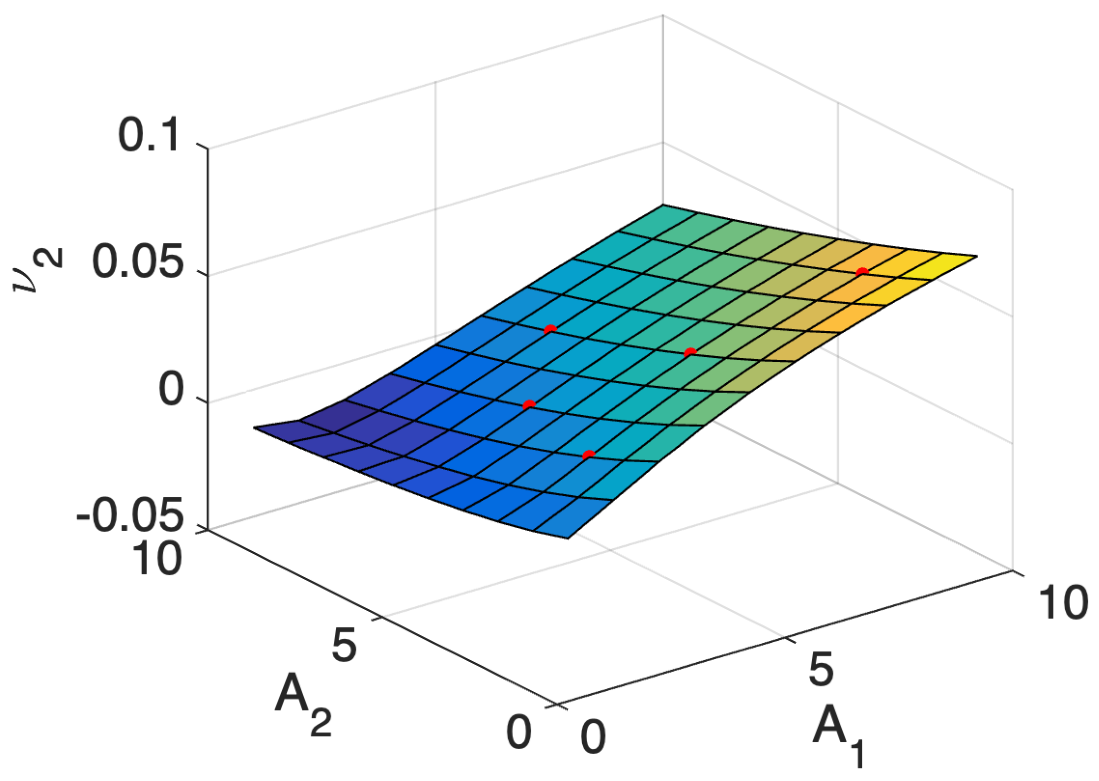
and by the flux expressions (26). An exploration of these stationary points is represented by Figure 2 and Figure 3. The reported 3D-surfaces show the domains of the admissible points ( [ A 1 ] , [ A 2 ] , ν 2 ) and ( [ S A 1 ] , [ S A 2 ] , ν 2 ) associated to a numerical exploration for the pair [ A 1 ] , [ A 2 ] in the set [ 1 , 10 ] × [ 1 , 10 ] mM. Note that the figures actually show the whole steady-state flux distribution related to the admissible vector of metabolites ( [ S A 1 ] , [ S A 2 ] , [ A 1 ] , [ A 2 ] ) since the constraint ν 1 = ν 2 = ν 3 holds at steady state.
Let us now assume to be able to infer (both experimentally and theoretically) M metabolic steady states including the related flux distributions. Let us assume for simplicity an ideal measurement process, meaning that the measured quantities are not corrupted by any kind of measurement error. To simulate this knowledge it is enough to randomly choose M different points on the 3D-domain ( [ A 1 ] , [ A 2 ] , ν 2 ) of Figure 3. The red dots reported in Figure 2 and Figure 3 represent these ideal measurements. In particular, we selected M = 5 random external conditions ( [ S A 1 ] , [ S A 2 ] ), and for each of them, we derived the complete knowledge of the corresponding internal quantities ( [ A 1 ] , [ A 2 ] , ν 1 , ν 2 , ν 3 ). Note that the choice of the number of steady states is not casual. In our example, reactions 1 and 3 are characterized by four unknown parameters each, p j = 4 , j = 1 , 3 , while reaction 2 is characterized by five parameters, p 2 = 5 , because of the considered activation mechanism. Therefore, according to Proposition 1 we set M = max { p 1 , p 2 , p 3 } = p 2 = 5 . This means that we need at least five different measurement sets (collecting concentrations and fluxes) to provide the minimal amount of information required by reaction 2. However, note that only 4 sets are actually required for the identification of the kinetic parameters of reactions 1 and 3. Therefore, in this deterministic case, M = 5 experimental points are enough to provide 13 independent algebraic constraints required to determine the 13 unknown parameters of the vector (28). Table 3 reports the five random points of Figure 2 and Figure 3, where P ( l ) = ( [ S A 1 ] ( l ) , [ S A 2 ] ( l ) , [ A 1 ] ( l ) , [ A 2 ] ( l ) , ν 1 ( l ) , ν 2 ( l ) , ν 3 ( l ) ) denotes the l-th point (removing the bar over the variables to simplify the notation).
Once the metabolic steady states P ( l ) , l = 1 , , 5 are known, the solution of the alternative identification method consists in finding the parameter vector (28) that satisfies the following algebraic system
h 1 f [ S A 1 ] ( l ) K 1 f h 1 b [ A 1 ] ( l ) K 1 b 1 + [ S A 1 ] ( l ) K 1 f + [ A 1 ] ( l ) K 1 b [ E 1 ] ( l ) ν 1 ( l ) = 0 , l = 1 , , 4 ,
h 3 f [ A 2 ] ( l ) K 3 f h 3 b [ S A 2 ] ( l ) K 3 b 1 + [ A 2 ] ( l ) K 3 f + [ S A 2 ] ( l ) K 3 b [ E 3 ] ( l ) ν 3 ( l ) = 0 , l = 1 , , 4 ,
[ A 1 ] ( k ) [ A 1 ] ( k ) + K A h 2 f [ A 1 ] ( k ) K 2 f h 2 b [ A 2 ] ( k ) K 2 b 1 + [ A 1 ] ( k ) K 2 f + [ A 2 ] ( k ) K 2 b [ E 2 ] ( k ) ν 2 ( k ) = 0 , k = 1 , , 5 .
Recall that the enzyme concentrations [ E 1 ] ( l ) , [ E 2 ] ( l ) , [ E 3 ] ( l ) , l = 1 , , 5 are assumed to be constant and known for all the metabolic states, and in particular equal to the random values given by Equation (30) for any l. As discussed in the previous sections, when the fluxes are known the parameter identification can be decoupled into smaller identification problems, one for each reaction. So in our example, since the fluxes are actually measured, the general system (31) is decoupled into the three smaller subsystems (32)–(34) (two of dimension 4 and one of dimension 5) and solved independently of each other. The algebraic subsystems are solved by using the MATLAB solver for nonlinear systems fsolve starting from the initial guess θ 0 with entries all equal to 10. The obtained solution θ ^ basically coincides with the true parameter vector reported in Table 2. For each kinetic parameter j, the computation shows a negligible relative error ( θ ^ j θ j ) / θ j of at most 10 6 .
Note that the uniqueness of the solution in a neighborhood of the initial guess θ 0 can be a priori verified by using the result of Section 4. Let us rewrite the algebraic subsystems (32)–(34) in the form
ξ 1 f [ S A 1 ] ( l ) ξ 1 b [ A 1 ] ( l ) [ E 1 ] ( l ) ν 1 ( l ) 1 + γ 1 f [ S A 1 ] ( l ) + γ 1 b [ A 1 ] ( l ) = 0 ,
ξ 3 f [ A 2 ] ( l ) ξ 3 b [ S A 2 ] ( l ) [ E 3 ] ( l ) ν 3 ( l ) 1 + γ 3 f [ A 2 ] ( l ) + γ 3 b [ S A 2 ] ( l ) = 0 ,
with l = 1 , , 4 , for reactions 1, 3, and in the form
ξ 2 f [ A 1 ] ( k ) ξ 2 b [ A 2 ] ( k ) [ A 1 ] ( k ) [ E 2 ] ( k ) ν 2 ( k ) ( [ A 1 ] ( k ) + K A ) 1 + γ 2 f [ A 1 ] ( k ) + γ 2 b [ A 2 ] ( k ) = 0 ,
with k = 1 , , 5 , for reaction 2, where some kinetic parameters have been redefined as
ξ j f = h j f K j f , ξ j b = h j b K j b , γ j f = 1 K j f , γ j b = 1 K j b .
Note that the parameter transformation (38) is invertible, so that if the new parameter vectors θ ˜ j = ( ξ j f , ξ j b , γ j f , γ j b ) T , j = 1 , 3 , and  θ ˜ 2 = ( ξ 2 f , ξ 2 b , γ 2 f , γ 2 b , K A ) T are identifiable then the original vectors θ j = ( h j f , h j b , K j f , K j b ) T , j = 1 , 3 , and  θ 2 = ( h 2 f , h 2 b , K 2 f , K 2 b , K A ) T are identifiable too.
The subsystems (35) and (36) are linear w.r.t. the new parameters θ ˜ j , j = 1 , 3 , so that the Jacobian matrices are independent of θ ˜ j . This property guarantees that the rank condition is independent of the initial parameter guess and then the local result given by Theorem 1 becomes actually global for reactions 1 and 3.
In particular, according to the artificial experimental measurements given in Table 3 and in Equation (30), we get the following numerical Jacobian matrices
J θ ˜ 1 = 42.6484 28.2418 0.0290 0.0192 121.0374 63.5441 0.8823 0.4632 65.5974 42.3628 0.0958 0.0618 71.7539 42.3628 0.2920 0.1724 ,
J θ ˜ 3 = 16.6154 43.7084 0.0288 0.0757 8.3077 16.8968 0.1544 0.3140 22.1538 57.1698 0.0825 0.2128 11.0769 25.9943 0.1149 0.2697 ,
computed independently of the initial guess θ 0 , and 
J θ ˜ 2 = 5.0933 7.6399 0.2685 0.4027 0.4842 25.7846 8.5949 8.8010 2.9337 6.2276 11.4598 15.2798 0.9895 1.3194 1.4534 11.4598 7.6399 2.7582 1.8388 2.9018 2.8650 2.8650 0.4268 0.4268 0.6675
which has been computed also on the basis of the value of θ 0 . The three Jacobians have full rank (indeed det ( J θ ˜ 1 ) = 0.0150 , det ( J θ ˜ 2 ) = 0.4105 , det ( J θ ˜ 3 ) = 0.0179 ) so providing the global identifiability of θ ˜ 1 and θ ˜ 3 , as well as of θ 1 and θ 3 , and the local identifiability of θ ˜ 2 , and then of θ 2 .
We remark that the number of multiple metabolic steady states required to completely determine the solution of the alternative method when the fluxes are known is independent of the network complexity. In the case of single-substrate/single-product reactions, as in our example, it is required the knowledge of at least 4 metabolic steady states in the absence of regulation or at least 5 steady states for the reaction with the activation mechanism. More in general, in the absence of regulation, such a minimal number is 2 + max { n j , j = 1 , 2 , , r } , where n j is the number of metabolites involved in reaction j; this number is increased for regulated reactions, as the dimension of the unknown parameter vector is extended by the kinetic parameters introduced by the regulation mechanism. Note that this minimal number is generally low (not far from 4–5) since typical reaction mechanisms usually involve few metabolites per reaction side (at most 2 or 3).
Let us now show the problems related to the classical time-course estimation problem. Assume that for the metabolic state 1, characterized by the external conditions [ S A 1 ] ( 1 ) = 6.04 , [ S A 2 ] ( 1 ) = 15.78 mM, we are able to measure some time samples from the time course of [ A 1 ] , [ A 2 ] . It should be possible to estimate the kinetic parameters (28) once a suitable number of time samples has been measured, using the classical approach of the minimization between the measures and the predictions of these measures, obtained by integrating ODE system (27). Let us reasonably assume that the external metabolite concentrations [ S A 1 ] ( 1 ) , [ S A 2 ] ( 1 ) are constant over time and that we know such values, after measuring them (always neglecting the measurement noise). Analogously to the alternative identification method, the enzyme concentrations [ E 1 ] ( 1 ) , [ E 2 ] ( 1 ) , [ E 3 ] ( 1 ) are assumed to be fixed over time and completely known; their values are again the random numbers given by (30). However, the unknowns of the time-course estimation problem are not the kinetic parameters only. Indeed, even if the kinetic parameters (that we are going to estimate), as well as the enzyme and external metabolite concentrations, were completely known, such knowledge would not be enough to integrate the dynamical system (27), since the initial state would actually be required. In fact, while the stationary values of [ A 1 ] , [ A 2 ] are independent of [ A 1 ] 0 , [ A 2 ] 0 , their transient time courses deeply depend on such initial conditions. This means that to avoid arbitrary choices of the initial state, we need to estimate both kinetic parameters and initial conditions. This is actually a remarkable drawback of this method, especially dealing with wide and complex networks. Indeed, even if this aspect has a small impact in terms of computational burden in small networks involving only a few metabolites, like the toy one considered here, for more complex networks balancing a huge number of metabolites such that an increase in unknowns could be not negligible. Last but not least, such an increase in the degrees of freedom has actually a significant impact on the identifiability properties of the time-course estimation problem.
Coming back to the specific example, the total number of unknowns to be estimated from the time samples is actually 15:13 kinetic parameters plus 2 initial conditions. So, to accomplish the least square estimation problem we need at least the same number of time samples.
Let us assume the same true values of the kinetic parameters hypothesized above (see the true parameters reported in Table 2) and the following random true values of the initial state
[ A 1 ] 0 = 9.17 , [ A 2 ] 0 = 2.86 ,
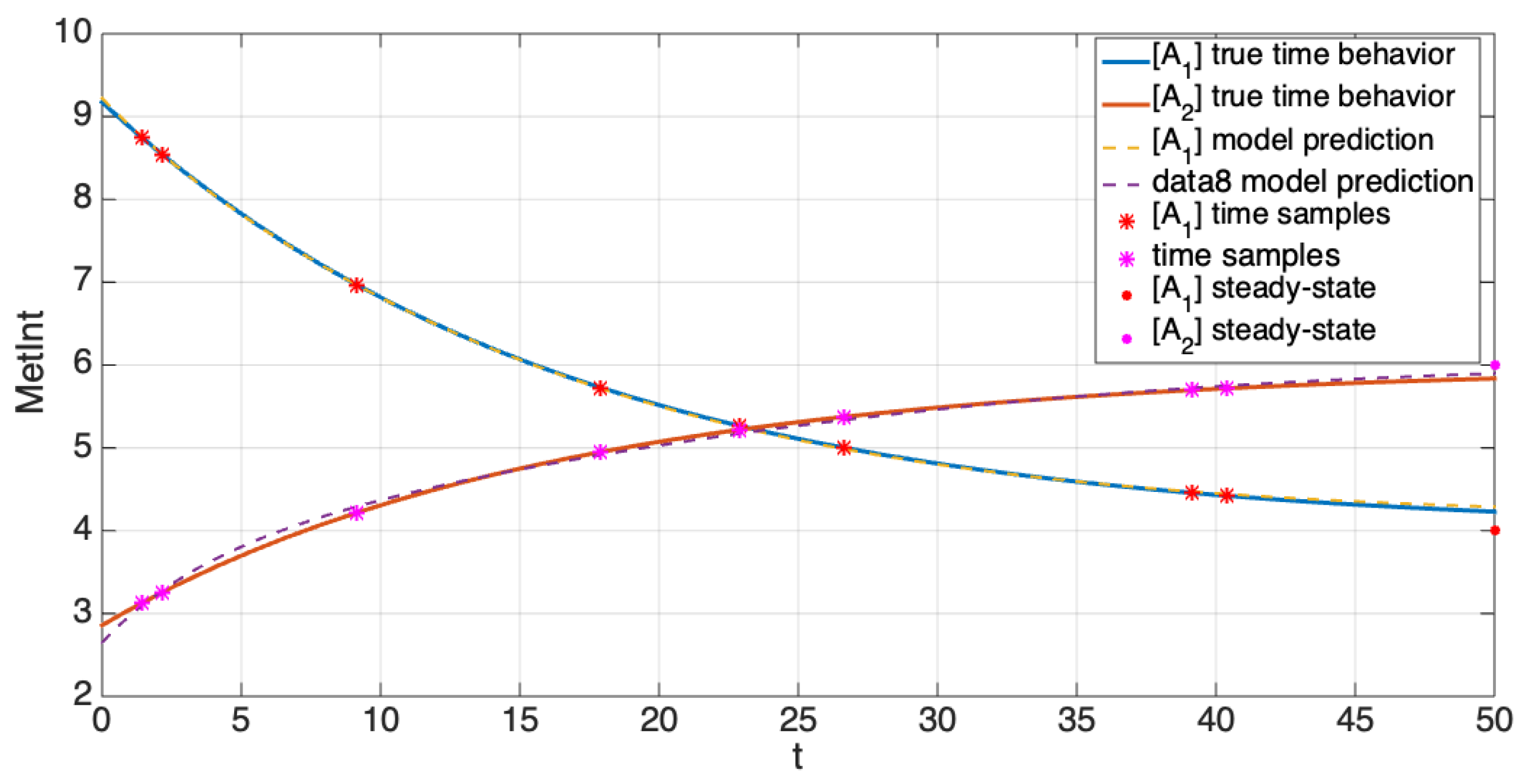
drawn from a uniform distribution over the interval [0, 10] mM. The chosen numerical set of parameter true values, together with the known fixed enzyme and external metabolite concentrations, provides the time course of [ A 1 ] , [ A 2 ] reported in Figure 4 (solid lines).
Let us assume, for instance, that we are able to measure the two-time profiles of [ A 1 ] , [ A 2 ] in 8 different time instants within the interval [0, 50]. Note that the chosen time span is the one providing the maximal information on the metabolite dynamics since both [ A 1 ] , [ A 2 ] have almost reached their stationary values at t = 50 and no significant change is obtained after this instant (compare the solid lines at t = 50 with the steady state values depicted by the solid circles in Figure 4). We also want to notice that an experiment collecting 8 time samples is actually a very optimistic situation compared to more usual experiments measuring shorter time series (usually 2–3 time samples). Assuming again an ideal measurement process (without measurement noise), we simulated such time samples by randomly selecting 8 points from each internal metabolite time course. The random time measurements are reported in Table 4, where the vector of the selected random time instants is denoted by t ˜ , while [ A 1 ] ˜ , [ A 2 ] ˜ are used for the corresponding vectors of the concentration samples. The artificial measurements are also depicted by the stars over the solid lines in Figure 4.
The numerical solution of the least square minimization problem between the measures [ A 1 ] ˜ , [ A 2 ] ˜ and the model predictions in the same instants t ˜ is obtained by means of the minimization routine fminsolve of MATLAB. For a fair comparison between the two estimation approaches, we initialize the minimization of the fminsolve using the same initial guess θ 0 used above in the alternative estimation (i.e., all the entries of θ 0 are set to 10). The minimization results are reported in Table 5, where the parameter vector estimated by means of the classical time-dependent approach is denoted by θ ^ ^ . For the sake of direct comparisons, Table 5 also reports the true parameter vector θ and the estimation obtained by means of the alternative approach θ ^ .
Moreover, the initial condition estimated by the classical approach is given by
[ A 1 ^ ^ ] 0 = 9.22 , [ A 2 ^ ^ ] 0 = 2.65 .
Comparing the estimated parameter vector θ ^ ^ with the true vector θ , as well as the model prediction with the true behavior, represented respectively by dashed and solid lines in Figure 4, it is evident that the time-course estimation problem has several minimum points. Indeed, the estimated parameters are far from the true values (at least for the kinetic parameters) while the model predictions are practically perfect. This result proves that the information content carried out by the time samples is not enough to provide a reliable estimation of the kinetic parameters. Probably, we need to increase the number of time samples or consider different time profiles related to multiple metabolic states, similar to the alternative identification method.

5.2. Two-Step Decomposition of the Alternative Estimation When Fluxes Are Partially Known

This second example illustrates how the computational complexity of the alternative estimation problem can be progressively reduced when partial flux knowledge is available.
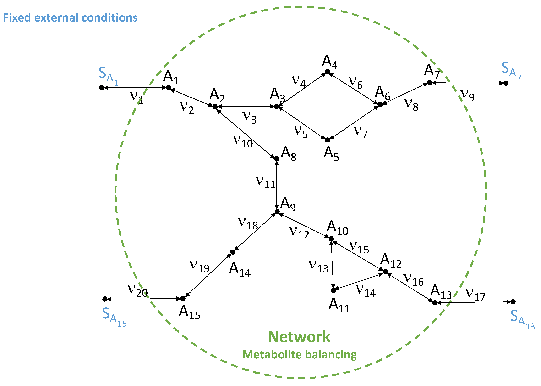
Let us consider the metabolic network given in Figure 5 including 15 internal metabolites, described by the concentrations [ A i ] , i = 1 , , 15 , and 20 reactions, characterized by the fluxes ν i , i = 1 , , 20 . Let us use the MM scheme to model all the kinetic mechanisms of the network reactions. This modeling choice introduces four kinetic parameters for each reaction (as the reactions are one-to-one and bidirectional), and then 80 unknowns are to be identified. Without a proper network decomposition, the computational burden of the identification task is high and unavoidably increases when the network dimension increases too (or if a more complex kinetic mechanism is taken into account). Conversely, when some network fluxes are known, the alternative identification allows decoupling of the original identification problem into smaller subproblems, so allowing us to easily study larger networks.
As shown by the simple example given in Section 5.1, when a bidirectional MM scheme (involving only two metabolites) is assumed, the alternative estimation requires four measured steady-states to estimate the unknown parameters, at least for the reactions with known fluxes. Therefore, let us assume to measure four steady-states (related to four different external conditions), i.e., four sets of internal metabolite concentrations ( [ A i ] ( l ) , i = 1 , , 15 , l = 1 , , 4 ) and some fluxes. Let us assume that the measurable fluxes are only the exchange ones, that is ν 1 ( l ) , ν 9 ( l ) , ν 17 ( l ) , ν 20 ( l ) , l = 1 , , 4 . Combining the flux measurements with the steady-state system (3) it is possible to uniquely determine a subset of flux values within the whole network. In particular, given the stoichiometry matrix
N T = 1 0 0 0 0 0 0 0 0 0 0 0 0 0 0 1 1 0 0 0 0 0 0 0 0 0 0 0 0 0 0 1 1 0 0 0 0 0 0 0 0 0 0 0 0 0 0 1 1 0 0 0 0 0 0 0 0 0 0 0 0 0 1 0 1 0 0 0 0 0 0 0 0 0 0 0 0 0 1 0 1 0 0 0 0 0 0 0 0 0 0 0 0 0 1 1 0 0 0 0 0 0 0 0 0 0 0 0 0 0 1 1 0 0 0 0 0 0 0 0 0 0 0 0 0 0 1 0 0 0 0 0 0 0 0 0 1 0 0 0 0 0 1 0 0 0 0 0 0 0 0 0 0 0 0 0 0 1 1 0 0 0 0 0 0 0 0 0 0 0 0 0 0 1 1 0 0 0 0 0 0 0 0 0 0 0 0 0 0 1 1 0 0 0 0 0 0 0 0 0 0 0 0 0 0 1 1 0 0 0 0 0 0 0 0 0 0 0 0 1 0 1 0 0 0 0 0 0 0 0 0 0 0 0 0 0 1 1 0 0 0 0 0 0 0 0 0 0 0 0 0 0 1 0 0 0 0 0 0 0 0 0 0 1 0 0 0 0 1 0 0 0 0 0 0 0 0 0 0 0 0 0 0 1 1 0 0 0 0 0 0 0 0 0 0 0 0 0 0 1 ,
system (3) provides the following relations
ν 2 = ν 1 , ν 3 = ν 8 = ν 9 , ν 12 = ν 16 = ν 17 , ν 18 = ν 19 = ν 20 , ν 10 = ν 11 = ν 17 + ν 20 ,
that allow to uniquely compute 13 flux values out of the 20 unknown fluxes, for each measured exchange set { ν 1 ( l ) , ν 9 ( l ) , ν 17 ( l ) , ν 20 ( l ) } , l = 1 , , 4 .
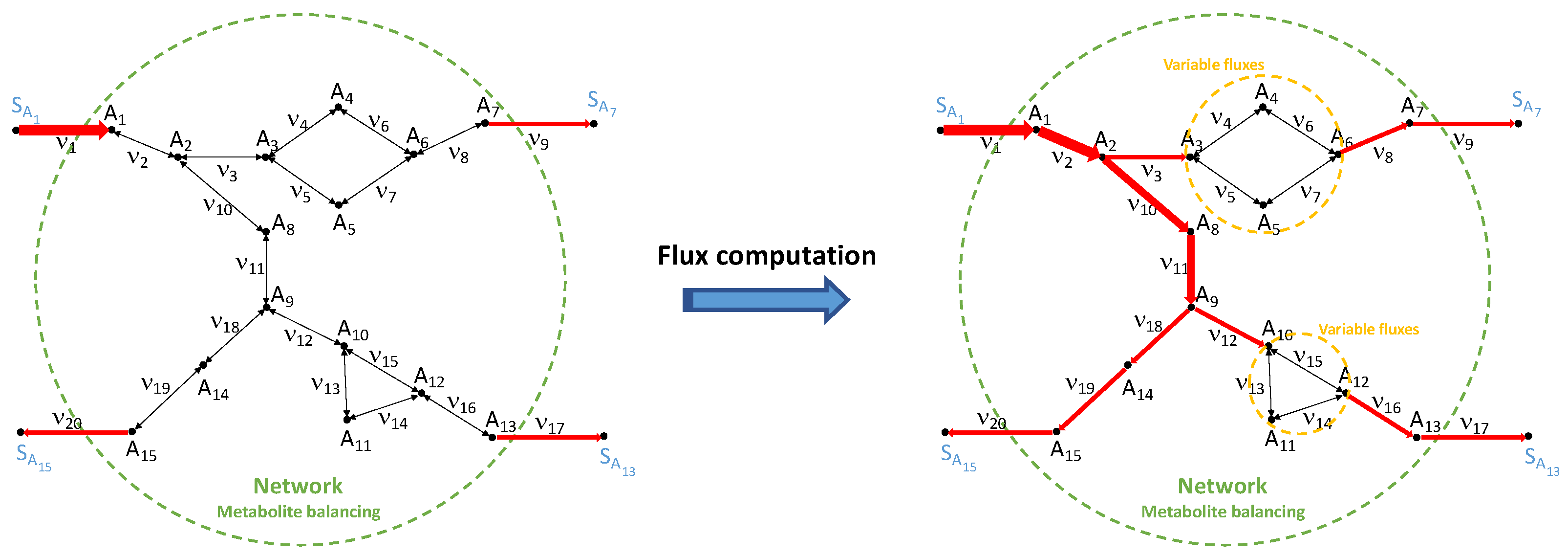
Figure 6 gives an illustrative example of a flux distribution obtained from a particular configuration of exchange fluxes ( ν 1 ( 1 ) = 0.15 mM/s, ν 9 ( l ) = 0.05 mM/s, ν 17 ( l ) = 0.05 mM/s, ν 20 ( l ) = 0.05 mM/s), where the fluxes having a unique value are marked by red arrows (the thickness of each arrow is proportional to the corresponding flux value). However, knowledge of the exchange fluxes only does not allow us to uniquely determine the whole flux distribution. Indeed, the 7 fluxes belonging to the subnetworks highlighted by the orange circles in Figure 6 are characterized by the following (independent) subsystems
ν 4 = ν 6 , ν 5 = ν 7 , ν 6 + ν 7 = ν 9 ,
and
ν 13 = ν 14 , ν 14 + ν 15 = ν 17 ,
that admit 1 solutions each (as the exchange fluxes ν 9 , ν 17 are known).
So thanks to this partial knowledge of fluxes, the global identification task of the 80 parameters can be decoupled into two steps. The first one consists of the identification of the kinetic parameters of the 13 reactions characterized by a unique flux value. As seen in the example of Section 5.1, the knowledge of fluxes (in addition to the metabolite concentrations) allows estimating the kinetic parameters of each reaction independently of the other ones. So, we do not need to solve a unique algebraic system of 52 unknowns but 13 independent and simpler subsystems of only 4 polynomial equations (of degree 2). As evidenced in the example of the previous section, in addition to the reduction of the computation burden, another advantage of this decomposition is that we can provide a global identifiability condition and a unique solution for each polynomial subsystem.
The second step of the identification consists in estimating the remaining 28 unknown parameters, related to the 7 reactions characterized by variable fluxes. However, such a second step benefits from the results of the previous identification. Indeed, a further decoupling of the 7 reactions left can be done thanks to the obtained flux distributions. In particular, two separated algebraic subsystems, one made by the kinetic parameters of reactions 4, 5, 6, 7 (16 unknowns), and the other one collecting the parameters of reactions 13, 14, 15 (12 unknowns), can be solved instead of a unique system of 28 unknowns (see Figure 7).
This further decomposition is a straightforward consequence of the flux distribution obtained in the previous step, which identifies two subnetworks (with variable fluxes) actually separated from each other. Moreover, the fluxes ν 3 , ν 8 , ν 12 , ν 16 known from the previous step are actually exchange fluxes for the two subnetworks and they can be used in the second identification step, in addition to the metabolite concentrations.

6. Conclusions

In the present paper, we deeply investigate the mathematical implications of the parameter identification approach proposed by Liebermeister and Klipp, 2006 [5,6]. Differently from the classical identification methods, the present one exploits only steady-state measurements, but related to several external conditions. The knowledge of multiple steady states is necessary to implement this approach since the number of kinetic parameters is usually much larger than the number of internal metabolites of the network.
The current investigation provides conditions to solve the proposed identification problem, as the number of required steady-state measurements and a theoretical result for the parameter identifiability. The mentioned theoretical result holds, in general, for any kinetic metabolic model, with any choice of the kinetic rate law. However, a simple clarifying example shows that for simple standard rate laws, as one-to-one Michaelis-Menten (but this is particularly true even for simpler mechanisms, as mass action), the result is actually stronger, providing the global identifiability of the unknown parameter vector. However, when the identifiability result holds only locally, the initial guess of the unknown parameters becomes actually crucial. In this case, an a priori knowledge is required (even though quite general), as done in the seminal paper [6] where ranges, mean values, or even general probability distributions are given for each category of parameters.
We also highlight many advantages of solving this type of identification problem. First of all, in the absence of measurement errors, the estimation problem consists in solving a nonlinear algebraic system which is polynomial, provided that the kinetic rate laws are chosen among the standard kinetic mechanisms (as mass-action, Michaelis–Menten, convenience rates). Moreover, the steady-state estimation requires a lower number of measurements than the classical one; the required measurements are metabolite concentrations at steady state, which are easier to be obtained w.r.t. time-course measurements. Finally, the proposed method becomes easier when both metabolite concentrations and fluxes are known. Indeed, the complexity of the identification problem can be reduced in this case, by decoupling the global estimation problem into smaller and simpler problems related to the single reactions. This decomposition highlights modular and symmetrical properties of the algebraic system and it is extremely relevant since it decreases the computational burden and allows for further reduce the number of required steady-state measurements. This is the main advantage of the proposed approach, introducing symmetries and modularities in the network structure, allowing to reduce the complexity of the identification task.
Future development of the present theoretical study is the application of the alternative identification method, as well as the identifiability results and the system decoupling, to a real case application, exploiting also real metabolic measurements.

Author Contributions

Conceptualization, G.P., A.B., F.P. and P.P.; methodology, G.P., A.B., F.P., M.P. and P.P.; software, F.P.; validation, G.P., A.B., F.P. and P.P.; formal analysis, G.P., A.B., F.P. and P.P.; investigation, F.P.; writing—original draft preparation, G.P., A.B., F.P. and P.P.; writing—review and editing, G.P., A.B., F.P. and P.P.; visualization, F.P. All authors have read and agreed to the published version of the manuscript.

Funding

This research received no external funding.

Data Availability Statement

No experimental data are used.

Conflicts of Interest

The authors declare no conflict of interest.

References

  1. Saa, P.A.; Nielsen, L.K. Formulation, construction and analysis of kinetic models of metabolism: A review of modelling frameworks. Biotechnol. Adv. 2017, 35, 981–1003. [Google Scholar] [CrossRef] [PubMed] [Green Version]
  2. Ibarra, R.U.; Edwards, J.S.; Palsson, B.Ø. Escherichia coli K-12 undergoes adaptive evolution to achieve Silico predicted optimal growth. Nature 2002, 420, 186–189. [Google Scholar] [CrossRef] [PubMed]
  3. Schuetz, R.; Zamboni, N.; Zampieri, M.; Heinemann, M.; Sauer, U. Multidimensional optimality of microbial metabolism. Science 2012, 336, 601–604. [Google Scholar] [CrossRef] [PubMed] [Green Version]
  4. Li, C.; Donizelli, M.; Rodriguez, N.; Dharuri, H.; Endler, L.; Chelliah, V.; Li, L.; He, E.; Henry, A.; Stefan, M.I.; et al. BioModels Database: An enhanced, curated and annotated resource for published quantitative kinetic models. BMC Syst. Biol. 2010, 4, 92. [Google Scholar] [CrossRef] [PubMed] [Green Version]
  5. Liebermeister, W.; Klipp, E. Bringing metabolic networks to life: Convenience rate law and thermodynamic constraints. Theor. Biol. Med. Model. 2006, 3, 41. [Google Scholar] [CrossRef] [PubMed] [Green Version]
  6. Liebermeister, W.; Klipp, E. Bringing metabolic networks to life: Integration of kinetic, metabolic, and proteomic data. Theor. Biol. Med. Model. 2006, 3, 42. [Google Scholar] [CrossRef] [PubMed] [Green Version]
  7. Feist, A.M.; Henry, C.S.; Reed, J.L.; Krummenacker, M.; Joyce, A.R.; Karp, P.D.; Broadbelt, L.J.; Hatzimanikatis, V.; Palsson, B.O. A genome-scale metabolic reconstruction for Escherichia coli K-12 MG1655 that accounts for 1260 ORFs and thermodynamic information. Mol. Syst. Biol. 2007, 3, 121. [Google Scholar] [CrossRef] [PubMed]
  8. Herrgard, M.J.; Swainston, N.; Dobson, P.; Dunn, W.B.; Arga, K.Y.; Arvas, M.; Blüthgen, N.; Borger, S.; Costenoble, R.; Heinemann, M.; et al. A consensus yeast metabolic network reconstruction obtained from a community approach to systems biology. Nat. Biotechnol. 2008, 26, 1155–1160. [Google Scholar] [CrossRef] [PubMed]
  9. Feist, A.M.; Palsson, B.Ø. The growing scope of applications of genome-scale metabolic reconstructions using Escherichia coli. Nat. Biotechnol. 2008, 26, 659–667. [Google Scholar] [CrossRef] [PubMed] [Green Version]
  10. Tran, L.M.; Rizk, M.L.; Liao, J.C. Ensemble modeling of metabolic networks. Biophys. J. 2008, 95, 5606–5617. [Google Scholar] [CrossRef] [PubMed]
  11. Lubitz, T.; Schulz, M.; Klipp, E.; Liebermeister, W. Parameter Balancing in Kinetic Models of Cell Metabolism. J. Phys. Chem. B 2010, 114, 16298–16303. [Google Scholar] [CrossRef] [PubMed]
  12. Stanford, N.J.; Lubitz, T.; Smallbone, K.; Klipp, E.; Mendes, P.; Liebermeister, W. Systematic Construction of Kinetic Models from Genome-Scale Metabolic Networks. PLoS ONE 2013, 8, e79195. [Google Scholar] [CrossRef] [PubMed] [Green Version]
  13. Antoniewicz, M.R. Methods and advances in metabolic flux analysis: A mini-review. J. Ind. Microbiol. Biotechnol. 2015, 42, 317–325. [Google Scholar] [CrossRef] [PubMed]
  14. Klipp, E.; Liebermeister, W.; Wierling, C.; Kowald, A.; Lehrach, H.; Herwig, R. (Eds.) Systems Biology: A Textbook; Wiley: Hoboken, NJ, USA, 2009. [Google Scholar]
  15. Noor, E.; Flamholz, A.; Bar-Even, A.; Davidi, D.; Milo, R.; Liebermeister, W. The protein cost of metabolic fluxes: Prediction from enzymatic rate laws and cost minimization. PLoS Comput. Biol. 2016, 12, e1005167. [Google Scholar] [CrossRef] [PubMed] [Green Version]
  16. Orth, J.D.; Thiele, I.; Palsson, B.Ø. What is flux balance analysis? Nat. Biotechnol. 2010, 28, 245–248. [Google Scholar] [CrossRef] [PubMed]
  17. Wiechert, W. 13C metabolic flux analysis. Metab. Eng. 2001, 3, 195–206. [Google Scholar] [CrossRef] [PubMed]
  18. Quek, L.E.; Wittmann, C.; Nielsen, L.K.; Kromer, J.O. OpenFLUX: Efficient modelling software for 13C-based metabolic flux analysis. Microb. Cell Factories 2009, 8, 25. [Google Scholar] [CrossRef] [PubMed] [Green Version]
  19. Weitzel, M.; Noh, K.; Dalman, T.; Niedenfuhr, S.; Stute, B.; Wiechert, W. 13CFLUX2—High-performance software suite for 13C-metabolic flux analysis. Bioinformatics 2013, 29, 143–145. [Google Scholar] [CrossRef] [PubMed] [Green Version]
  20. Young, J.D. INCA: A computational platform for isotopically non-stationary metabolic flux analysis. Bioinformatics 2014, 30, 1333–1335. [Google Scholar] [CrossRef] [PubMed]
  21. Allendoerfer, C.B. (Ed.) Calculus of Several Variables and Differentiable Manifolds; Macmillan: New York, NY, USA, 1974. [Google Scholar]
  22. Ross, J.; Nyström, D.W. Differentiability of the argmin function and a minimum principle for semiconcave subsolutions. arXiv 2018, arXiv:1808.04402. [Google Scholar]
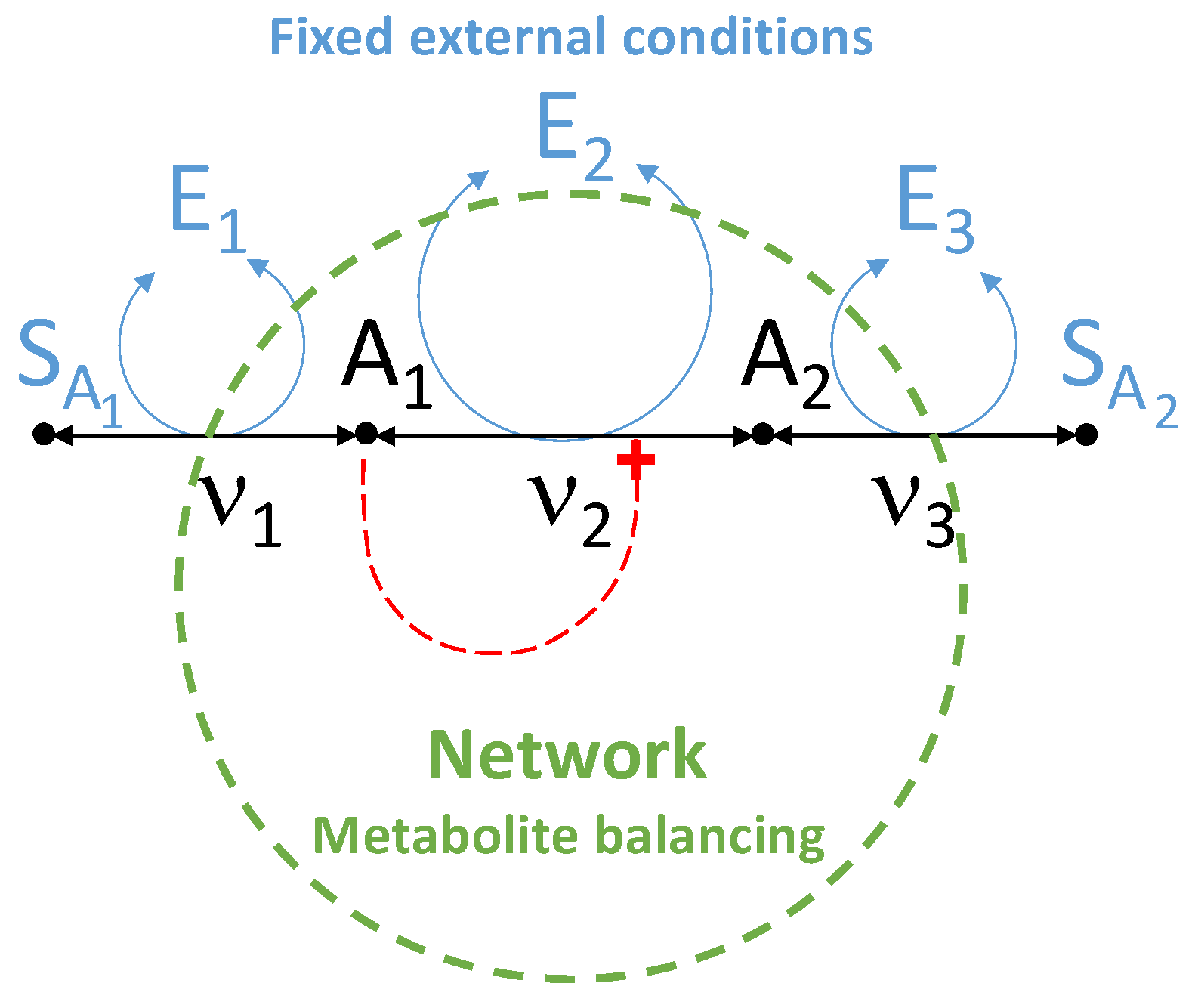
Figure 1. Toy metabolic network representing a conversion between two metabolites and accounting for an activation mechanism.
Symmetry 15 00368 g001
Figure 2. Steady-state flux distribution as a function of [ S A 1 ] , [ S A 2 ] .
Symmetry 15 00368 g002
Figure 3. Steady-state flux distribution as a function of [ A 1 ] , [ A 2 ] .
Symmetry 15 00368 g003
Figure 4. Time course of the internal metabolite concentrations [ A 1 ] , [ A 2 ] in [ 0 , 50 ] . Solid lines: true values; Stars: time samples (see Table 4); Dashed lines: model predictions based on the estimated parameters; Solid circle: stationary values. Enzyme concentrations given by Equation (30); External substrates: [ S A 1 ] ( 1 ) = 6.04 , [ S A 2 ] ( 1 ) = 15.78 mM; True kinetic parameters reported in Table 2; True initial conditions: [ A 1 ] 0 = 9.17 , [ A 2 ] 0 = 2.86 mM. The model predictions are obtained with the estimated kinetic parameters and initial condition reported in Table 5.
Symmetry 15 00368 g004
Figure 5. Metabolic network of 15 internal metabolites and 20 reactions. ν 1 , ν 9 , ν 17 , ν 20 are exchange fluxes.
Symmetry 15 00368 g005
Figure 6. Example of flux distribution obtained from the measured fluxes ν 1 ( 1 ) = 0.15 mM/s, ν 9 ( l ) = 0.05 mM/s, ν 17 ( l ) = 0.05 mM/s, ν 20 ( l ) = 0.05 mM/s. Thick arrows: 0.15 mM/s; medium arrows: 0.1 mM/s; thin arrows: 0.05 mM/s.
Symmetry 15 00368 g006
Figure 7. Subnetworks coming from the flux distribution computed in step one, characterized by known exchange fluxes.
Symmetry 15 00368 g007
Table 1. Number of parameters for different modeling choices.
Kinetic MechanismNumber of ParametersKinetic ParametersEquation
One-to-One Mass Action2 k f , k b (5)
One-to-One Michaelis Menten4 k f , k b , K f , K b (7)
n F -to- n B Convenience Rate 2 + n F + n B h f , h b ,
{ K i F , i = 1 , , n F } , { K i B , i = 1 , , n B } (8)
Regulation module1 K A (or K I )(9)
Table 2. True values of the kinetic parameters.
Kinetic ParameterTrue Value
h 1 f 0.0344
h 1 b 0.7655
K 1 f 0.4617
K 1 b 6.9483
h 2 f 0.4387
h 2 b 0.7952
K 2 f 0.9713
K 2 b 3.1710
K A 7.4484
h 3 f 0.3816
h 3 b 0.1869
K 3 f 7.2346
K 3 b 9.5022
Table 3. Artificial experimental points randomly selected on the 3D-domains of Figure 2 and Figure 3.
P 1 P 2 P 3 P 4 P 5
6.040517.14309.290810.16284.6702
15.78366.101620.64479.38687.6004
4.00009.00006.00006.00003.0000
6.00003.00008.00004.00003.0000
0.00480.05150.01030.02870.0109
0.00480.05150.01030.02870.0109
0.00480.05150.01030.02870.0109
Table 4. Artificial measurements of the time courses of [ A 1 ] and [ A 2 ] , randomly selected on the interval [ 0 , 50 ] .
t ˜ [ A 1 ] ˜ [ A 2 ] ˜
1.45268.74013.1321
2.17898.53713.2593
9.15516.96674.2182
17.90515.72704.9502
22.90515.26445.2205
26.65515.00005.3753
39.15514.45585.6979
40.40514.42135.7188
Table 5. True parameter vector θ vs the two estimators: alternative estimation θ ^ and classical time-dependent estimation θ ^ ^ .
Kinetic Parameter θ θ ^ θ ^ ^
h 1 f 0.03440.03440.2137
h 1 b 0.76550.76550.3171
K 1 f 0.46170.46176.7456
K 1 b 6.94836.94832.2505
h 2 f 0.43870.43873.8292
h 2 b 0.79520.79526.4673
K 2 f 0.97130.97136.4887
K 2 b 3.17103.17100.1928
K A 7.44847.44846.6438
h 3 f 0.38160.38161.9562
h 3 b 0.18690.18690.8278
K 3 f 7.23467.23466.4133
K 3 b 9.50229.50223.7288
Disclaimer/Publisher’s Note: The statements, opinions and data contained in all publications are solely those of the individual author(s) and contributor(s) and not of MDPI and/or the editor(s). MDPI and/or the editor(s) disclaim responsibility for any injury to people or property resulting from any ideas, methods, instructions or products referred to in the content.