On Fuzzy Linear Fractional Programming Problems via α-Cut-Based Method with Application in Transportation Sector

Abstract

The article provides an $\alpha$-cut-based method that solves linear fractional programming problems with fuzzy variables and unrestricted parameters. The parameters and variables are considered as asymmetric triangular fuzzy numbers, which is a generalization of the symmetric case. The problem is solved by using $\alpha$-cut of fuzzy numbers wherein the $\alpha$- and r-cut are applied to the objective function and constraints, respectively. This reduces the problem into an equivalent biobjective model which leads to the upper and lower bounds of the given problem. Afterwards, the membership functions corresponding to various values of $r\in (0,1]$ are obtained using the optimal values of the biobjective model. The proposed method is illustrated by taking an example from the literature to highlight the fallacy of an existing approach. Finally, a fuzzy linear fractional transportation problem is modelled and solved using the aforementioned technique.

1. Introduction

Linear programming problems (LPPs) are a significant type of optimization problems. These LPPs are used to solve various real-world problems such as production planning, hospital management, transportation problems, diet planning, profit maximization, resource management, etc. Linear fractional programming problems (LFPPs) are LPPs where the objective function is a ratio between two linear functions. Such LFPPs are widely used in economic and commercial models to maximize profit and minimize cost, simultaneously. In the literature, out of several ways to deal with LFPPs, some methods are analytical while some are numerical.

In a significant development, Charnes and Cooper [1] solved LFPPs by using an analytical variable transformation method that reduced the problem into LPPs with some added constraints. Tantawy [2] considered an iterative method to find an optimal solution by sequentially moving from an initial interior point to another feasible solution until the optimal solution is reached. Meanwhile, Chadha and Chadha [3] proved some results regarding the dual of an LFPP and expressed the dual to be an LPP, which was further solved to get a solution to the initial problem. Later, Rizk-Allah et al. [4] provided a new algorithm for linear and nonlinear fractional programming problems, viz., chaotic crow search algorithm. In addition to these, there are various methods based on the simplex approach to find solutions of LFPPs. Sharma and Bansal [5] used the branch-and-bound process along with the simplex technique to solve LFPPs. Next, Pandey and Punnen [6] generalized and extended existing simplex algorithms.

LFPPs can be used to frame many real-world problems, but in most cases, the data provided to the decision-maker are not clearly defined and precise. Generally, there is some form of uncertainty associated with the data. These uncertainties can be overcome by incorporating the fuzzy sense introduced by Zadeh [7] in the parameters, constraints or variables. Nowadays, fuzzy linear fractional programming problems (FLFPPs) are used instead of LFPPs to cater to real-world scenarios. Over time, a number of different techniques have been explored by researchers to solve FLFPPs. Hladík [8] and Borza et al. [9] studied generalized LFPPs with interval uncertainties. Later, Pandian and Jayalakshmi [10] solved LFPPs by a denominator restriction method, which further extended to a decomposition restriction method that solved the FLFPP by converting the problem into three crisp-level LFPPs. Further, Das and Mandal [11] as well as Das et al. [12] converted FLFPPs into crisp multiobjective LFPPs, which were then solved to obtain a solution. In one of their studies, Sharma et al. [13] considered multiobjective fractional programming problems for fixed aspiration levels using symmetric fuzzy parameters. Dutta et al. [14,15] worked on the sensitivity of FLFPPs and also investigated the impact of tolerance on both LFPPs and FLFPPs. Recently, Borza and Rambely [16] solved the FLFPPs with crisp variables and coefficients as TFNs by using a combination of the max-min method and an $\alpha$-cut-based approach.

Veeramani and Sumathi [17] suggested a method that converted the problem into a multiobjective LFPP and then solved it using the fuzzy programming approach. However, Mehra et al. [18] proposed the novel concept of $(\alpha ,\beta )$-acceptable optimal solution of an FLFPP having fuzzy coefficients. Further, Das et al. [19] proposed a new ordering for TFNs and used this to reduce an FLFPP into a triobjective problem. Meanwhile, Chinnadurai and Muthukumar [20] considered an FLFPP with all parameters and variables as triangular fuzzy numbers (TFNs) and proposed an $\alpha$-cut-based numerical approach to solve the problem by converting it into an equivalent biobjective model. They erroneously claimed to propose a method for any general FLFPP. Subsequently, Ebrahimnejad et al. [21] worked on a similar numerical approach with non-negative trapezoidal fuzzy numbers. In the present study, a counterexample is cited, which shows that the approach in [20] can be used only when all the parameters are non-negative TFNs. Further, we have established the conditions for the proposed $\alpha$-cut-based method to solve the above-mentioned FLFPPs having unrestricted parameters, which overcomes the shortcoming in [20].

The rest of the paper is structured as follows: Section 2 is dedicated to notations, definitions and arithmetic operations, used throughout this paper. Section 3 describes the formulation of a standard FLFPP having asymmetric TFNs. In Section 4, the approach in [20] is presented along with a counterexample to highlight its shortcoming. The motivation for the new approach and the limitations of existing approaches are indicated in Section 5. Next, Section 6 explains the proposed approach. Later, a numerical illustration and a real-world application are worked out using the proposed method in Section 7. The results are discussed in Section 8. Finally, conclusions and future scope are addressed in Section 9.

2. Notations and Definitions

Some preliminary notations and definitions used in the article are presented in this section.

Definition 1

([20]). If X is a collection of objects denoted generically by x, then a fuzzy set $\tilde{A}$ in X is a set of ordered pairs: $\left\{(x,{\mu }_{\tilde{A}}\left(x\right))|x\in X\right\},{\mu }_{\tilde{A}}$ is called the membership function of $\tilde{A}$ which maps X to $[0,1]$, and ${\mu }_{\tilde{A}}\left(x\right)$ is called the membership degree of x in $\tilde{A}$.

Definition 2

([20]). The (crisp) set of elements that belong to the fuzzy set $\tilde{A}$ at least to the degree $\alpha \in (0,1]$ is called the α-cut of $\tilde{A}$ and is defined as:

$${\left(\tilde{A}\right)}_{\alpha }=\{x\in X|{\mu }_{\tilde{A}}\left(x\right)\ge \alpha \}.$$

Definition 3

([22]). A fuzzy set $\tilde{A}$ in $\mathbb{R}$ is said to be a fuzzy number if

(i)

$\exists r\in \mathbb{R}$ such that ${\mu }_{\tilde{A}}\left(r\right)=1;$

(ii)

$\forall \alpha \in (0,1]$, ${\left(\tilde{A}\right)}_{\alpha }$ is a closed interval in $\mathbb{R}$, i.e., ${\left(\tilde{A}\right)}_{\alpha }=[{\left(\tilde{A}\right)}_{\alpha }^L,{\left(\tilde{A}\right)}_{\alpha }^U]⊊\mathbb{R}$;

(iii)

the set $R_0=\{r\in \mathbb{R}|{\mu }_{\tilde{A}}\left(r\right)>0\}$ is a finite subset of $\mathbb{R}.$

Arithmetic operations on closed intervals of $\mathbb{R}$

Let $I_1=[a_1,a_2]$ and $I_2=[b_1,b_2]$ be two closed intervals of $\mathbb{R}$; we define:

(i)

$I_1+I_2=[a_1+b_1,a_2+b_2].$

(ii)

$I_1-I_2=[a_1-b_2,a_2-b_1].$

(iii)

$\forall k\in \mathbb{R},k.I_1=\left\{\begin{array}{c}[k{a}_1,k{a}_2],k\ge 0,\hfill \\ {}_2,k{a}_1],k<0.\hfill \end{array}\right.$

(iv)

$I_1{I}_2=[p_1,p_2]$

where $p_1=min\{a_1{b}_1,a_1{b}_2,a_2{b}_1,a_2{b}_2\}$ and

$p_2=max\{a_1{b}_1,a_1{b}_2,a_2{b}_1,a_2{b}_2\}.$

(v)

$I_1/I_2=[q_1,q_2]$

where $q_1=min\{a_1/b_1,a_1/b_2,a_2/b_1,a_2/b_2\}$ and

$q_2=max\{a_1/b_1,a_1/b_2,a_2/b_1,a_2/b_2\}$, provided $0\notin I_2$.

Remark 1.

In particular, for $I_2=[b_1,b_2]$; $0<b_1\le b_2$,

$$[q_1,q_2]=\left\{\begin{array}{c}[a_1/b_2,a_2/b_1],a_1\ge 0,\hfill \\ {}_1/b_1,a_2/b_1],a_1<0\&a_2\ge 0,\hfill \\ {}_1/b_1,a_2/b_2],a_2<0.\hfill \end{array}\right.$$

(vi)

$I_1\ge I_2$ iff $a_1\ge b_1$ and $a_2\ge b_2.$

Ordering of fuzzy numbers: [20]. The ordering of fuzzy numbers is defined as follows:

(i)

$\tilde{A}⪰\tilde{B}$ iff $\forall \alpha \in (0,1],{\left(\tilde{A}\right)}_{\alpha }\ge {\left(\tilde{B}\right)}_{\alpha }$, i.e., $\forall \alpha \in (0,1],{\left(\tilde{A}\right)}_{\alpha }^L\ge {\left(\tilde{B}\right)}_{\alpha }^L$ and ${\left(\tilde{A}\right)}_{\alpha }^U\ge {\left(\tilde{B}\right)}_{\alpha }^U.$

(ii)

$\tilde{A}⪰0$ iff $\forall \alpha \in (0,1],{\left(\tilde{A}\right)}_{\alpha }^L\ge 0.$

Definition 4

([21]). A triangular fuzzy number (TFN) $\tilde{A}=(a,a^{\prime },a^{″})$ where $a\le a^{\prime }\le a^{″},$ is a fuzzy set in $\mathbb{R}$ if its membership function is given by

$${\mu }_{\tilde{A}}\left(x\right)=\left\{\begin{array}{c}\frac{x-a}{a^{\prime }-a}, a<x<a^{\prime },\hfill \\ 1, x=a^{\prime },\hfill \\ \frac{a^{″}-x}{a^{″}-a^{\prime }}, a^{\prime }<x<a^{″},\\ 0, otherwise.\end{array}\right.$$

For a TFN $\tilde{A}=(a,a^{\prime },a^{″})$:

(i)

${\left(\tilde{A}\right)}_{\alpha }=[{\left(\tilde{A}\right)}_{\alpha }^L,{\left(\tilde{A}\right)}_{\alpha }^U]=[a+\alpha (a^{\prime }-a),a^{″}-\alpha (a^{″}-a^{\prime })].$

(ii)

$\tilde{A}$ is a non-negative TFN $(\tilde{A}⪰0)$ iff $a+\alpha (a^{\prime }-a)\ge 0\forall \alpha \in (0,1]$, i.e., $a\ge 0$.

(iii)

$\tilde{A}$ is a positive TFN $(\tilde{A}\succ 0)$ iff $a+\alpha (a^{\prime }-a)>0\forall \alpha \in (0,1]$.

Clearly $\tilde{A}\succ 0\Rightarrow \tilde{A}⪰0.$

(iv)

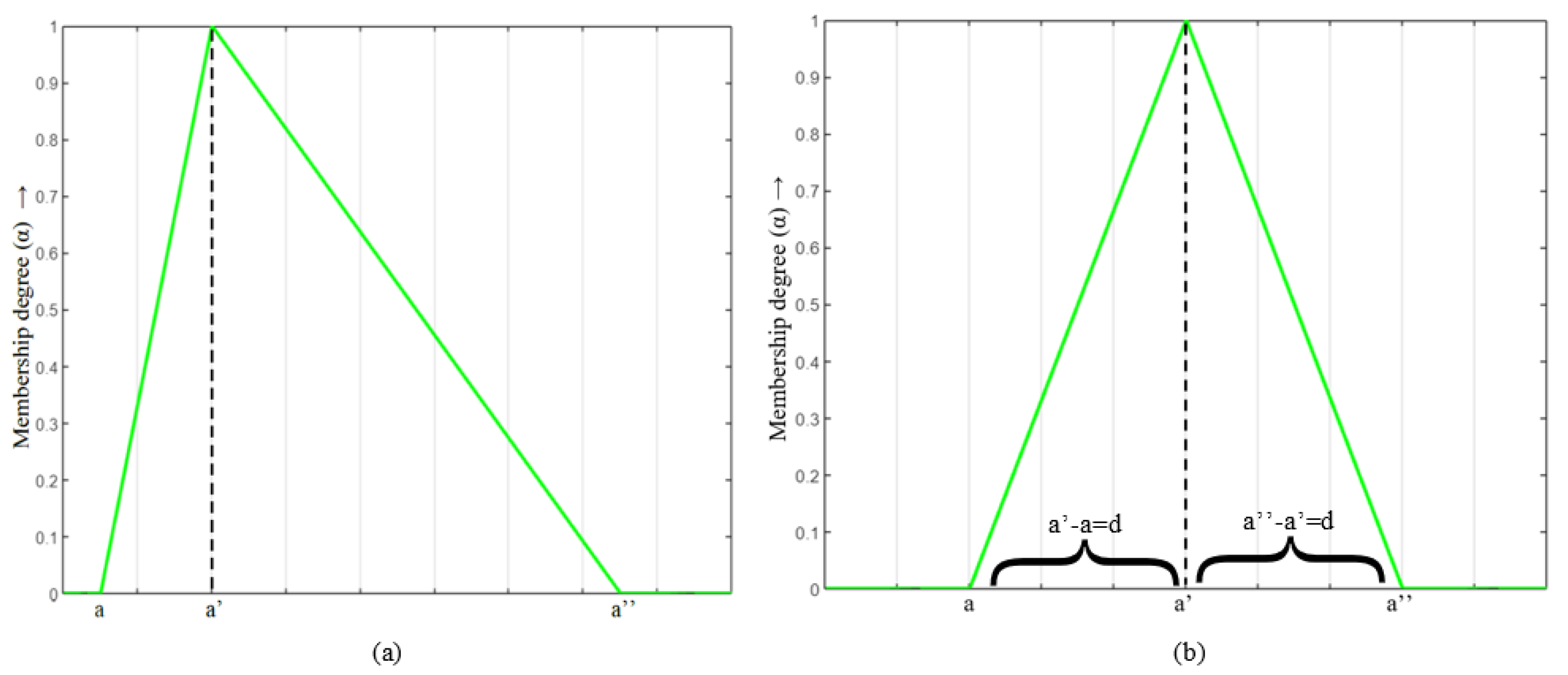
When $a^{\prime }-a=a"-a^{\prime }$$=d$, it is said to be symmetric else asymmetric TFN

(see Figure 1, [23]).

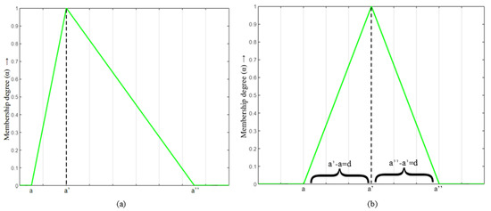Figure 1. Triangular fuzzy numbers: (a) asymmetric TFN; (b) symmetric TFN.

Definition 5.

A fuzzy number $\tilde{A}$ is said to be a negative TFN $(\tilde{A}\prec 0)$ if $\tilde{A}$ is not a non-negative TFN.

Let us denote the set of all TFNs in $\mathbb{R}$ as $T\left(\mathbb{R}\right)$. Further, let $T\left({\mathbb{R}}^{+}\right)$ and $T\left({\mathbb{R}}^{++}\right)$ be the collection of all non-negative and all positive TFNs, respectively, in $\mathbb{R}$. It follows that

$$T\left({\mathbb{R}}^{++}\right)⊊T\left({\mathbb{R}}^{+}\right)⊊T\left(\mathbb{R}\right).$$

Definition 6

([22]). Let $\tilde{A}$ be a fuzzy set defined on the universal set X. Then, for some $\alpha \in (0,1],{}^{\alpha }A$ is a fuzzy set defined on X as ${}^{\alpha }A=\left\{(x,{\mu }_{\left({}^{\alpha }A\right)}\left(x\right))\right|x\in X\}$, where

$${\mu }_{\left({}^{\alpha }A\right)}\left(x\right)=\left\{\begin{array}{cc}\alpha ,\hfill & x\in {\left(\tilde{A}\right)}_{\alpha },\hfill \\ 0,\hfill & x\notin {\left(\tilde{A}\right)}_{\alpha }.\hfill \end{array}\right.$$

Theorem 1

(First Decomposition Theorem [22]).

$$\mathit{For} \mathit{fuzzy}\mathit{ }\mathit{every} \mathit{set} \tilde{A},\tilde{A}={\bigcup }_{\alpha \in [0,1]}^{}{}^{\alpha }A$$

The first decomposition theorem states that any fuzzy set can be represented using its α-cut alone. Hence, to define arithmetic operations on TFNs, only the α-cut of the resulting fuzzy number is sufficient.

Arithmetic operations on α-cut of fuzzy numbers [20]:

Let ${\tilde{A}}_1$ and ${\tilde{A}}_2\in T\left(\mathbb{R}\right)$ with α-cut ${\left({\tilde{A}}_1\right)}_{\alpha }=[{\left({\tilde{A}}_1\right)}_{\alpha }^L,{\left({\tilde{A}}_1\right)}_{\alpha }^U]$ and ${\left({\tilde{A}}_2\right)}_{\alpha }=[{\left({\tilde{A}}_2\right)}_{\alpha }^L,{\left({\tilde{A}}_2\right)}_{\alpha }^U]$, respectively. Then, $\forall \alpha \in (0,1],$ the fuzzy arithmetic operations between ${\tilde{A}}_1$ and ${\tilde{A}}_2$ using the α-cut are defined as follows:

(i)

$\begin{array}{cc}\hfill \mathrm{Addition}: {({\tilde{A}}_1\oplus {\tilde{A}}_2)}_{\alpha }& ={\left({\tilde{A}}_1\right)}_{\alpha }+{\left({\tilde{A}}_2\right)}_{\alpha }\hfill \\ & =\left[{\left({\tilde{A}}_1\right)}_{\alpha }^L+{\left({\tilde{A}}_2\right)}_{\alpha }^L,{\left({\tilde{A}}_1\right)}_{\alpha }^U+{\left({\tilde{A}}_2\right)}_{\alpha }^U)\right].\hfill \end{array}$

(ii)

$\begin{array}{cc}\hfill \mathrm{Subtraction}: {({\tilde{A}}_1\ominus {\tilde{A}}_2)}_{\alpha }& ={\left({\tilde{A}}_1\right)}_{\alpha }-{\left({\tilde{A}}_2\right)}_{\alpha }\hfill \\ & =\left[{\left({\tilde{A}}_1\right)}_{\alpha }^L-{\left({\tilde{A}}_2\right)}_{\alpha }^U,{\left({\tilde{A}}_1\right)}_{\alpha }^U-{\left({\tilde{A}}_2\right)}_{\alpha }^L)\right].\hfill \end{array}$

(iii)

Scalar multiplication:

For any $k\in \mathbb{R},{(k\otimes {\tilde{A}}_1)}_{\alpha }=k{\left({\tilde{A}}_1\right)}_{\alpha }=\left\{\begin{array}{c}\left[k{\left({\tilde{A}}_1\right)}_{\alpha }^L,k{\left({\tilde{A}}_1\right)}_{\alpha }^U\right],k\ge 0,\hfill \\ \left[k{\left({\tilde{A}}_1\right)}_{\alpha }^U,k{\left({\tilde{A}}_1\right)}_{\alpha }^L\right],k<0.\hfill \end{array}\right.$

(iv)

$\begin{array}{cc}\hfill \mathrm{Multiplication}: {({\tilde{A}}_1\otimes {\tilde{A}}_2)}_{\alpha }& ={\left({\tilde{A}}_1\right)}_{\alpha }{\left({\tilde{A}}_2\right)}_{\alpha }\hfill \\ & =\left[{\left(\tilde{P}\right)}_{\alpha }^L,{\left(\tilde{P}\right)}_{\alpha }^U\right], \mathrm{where}\hfill \end{array}$

${\left(\tilde{P}\right)}_{\alpha }^L=\min \left\{{\left({\tilde{A}}_1\right)}_{\alpha }^L{\left({\tilde{A}}_2\right)}_{\alpha }^L,{\left({\tilde{A}}_1\right)}_{\alpha }^L{\left({\tilde{A}}_2\right)}_{\alpha }^U,{\left({\tilde{A}}_1\right)}_{\alpha }^U{\left({\tilde{A}}_2\right)}_{\alpha }^L,{\left({\tilde{A}}_1\right)}_{\alpha }^U{\left({\tilde{A}}_2\right)}_{\alpha }^U\right\}$ and

${\left(\tilde{P}\right)}_{\alpha }^U=\max \left\{{\left({\tilde{A}}_1\right)}_{\alpha }^L{\left({\tilde{A}}_2\right)}_{\alpha }^L,{\left({\tilde{A}}_1\right)}_{\alpha }^L{\left({\tilde{A}}_2\right)}_{\alpha }^U,{\left({\tilde{A}}_1\right)}_{\alpha }^U{\left({\tilde{A}}_2\right)}_{\alpha }^L,{\left({\tilde{A}}_1\right)}_{\alpha }^U{\left({\tilde{A}}_2\right)}_{\alpha }^U\right\}.$

Remark 2.

Let ${\tilde{A}}_2\in T\left({\mathbb{R}}^{++}\right)$, i.e., $0<{\left({\tilde{A}}_2\right)}_{\alpha }^L\le {\left({\tilde{A}}_2\right)}_{\alpha }^U,$ then

${\left(\tilde{P}\right)}_{\alpha }^L=min\left\{{\left({\tilde{A}}_1\right)}_{\alpha }^L{\left({\tilde{A}}_2\right)}_{\alpha }^L,{\left({\tilde{A}}_1\right)}_{\alpha }^L{\left({\tilde{A}}_2\right)}_{\alpha }^U\right\}$ and ${\left(\tilde{P}\right)}_{\alpha }^U=max\left\{{\left({\tilde{A}}_1\right)}_{\alpha }^U{\left({\tilde{A}}_2\right)}_{\alpha }^L,{\left({\tilde{A}}_1\right)}_{\alpha }^U{\left({\tilde{A}}_2\right)}_{\alpha }^U\right\}.$

(v)

$\begin{array}{cc}\hfill \mathrm{Division}: {({\tilde{A}}_1\oslash {\tilde{A}}_2)}_{\alpha }& ={\left({\tilde{A}}_1\right)}_{\alpha }/{\left({\tilde{A}}_2\right)}_{\alpha }\hfill \\ & =\left[{\left(\tilde{Q}\right)}_{\alpha }^L,{\left(\tilde{Q}\right)}_{\alpha }^U\right], \mathrm{where}\hfill \end{array}$

${\left(\tilde{Q}\right)}_{\alpha }^L=\min \left\{{\left({\tilde{A}}_1\right)}_{\alpha }^L/{\left({\tilde{A}}_2\right)}_{\alpha }^L,{\left({\tilde{A}}_1\right)}_{\alpha }^L/{\left({\tilde{A}}_2\right)}_{\alpha }^U,{\left({\tilde{A}}_1\right)}_{\alpha }^U/{\left({\tilde{A}}_2\right)}_{\alpha }^L,{\left({\tilde{A}}_1\right)}_{\alpha }^U/{\left({\tilde{A}}_2\right)}_{\alpha }^U\right\}$ and

${\left(\tilde{Q}\right)}_{\alpha }^U=\max \left\{{\left({\tilde{A}}_1\right)}_{\alpha }^L/{\left({\tilde{A}}_2\right)}_{\alpha }^L,{\left({\tilde{A}}_1\right)}_{\alpha }^L/{\left({\tilde{A}}_2\right)}_{\alpha }^U,{\left({\tilde{A}}_1\right)}_{\alpha }^U/{\left({\tilde{A}}_2\right)}_{\alpha }^L,{\left({\tilde{A}}_1\right)}_{\alpha }^U/{\left({\tilde{A}}_2\right)}_{\alpha }^U\right\}$, provided $0\notin {\left({\tilde{A}}_2\right)}_{\alpha }.$

Remark 3.

Let ${\tilde{A}}_1,{\tilde{A}}_2\in T\left({\mathbb{R}}^{+}\right)$, then

$$\left[{\left(\tilde{Q}\right)}_{\alpha }^L,{\left(\tilde{Q}\right)}_{\alpha }^U\right]=[{\left({\tilde{A}}_1\right)}_{\alpha }^L/{\left({\tilde{A}}_2\right)}_{\alpha }^U,{\left({\tilde{A}}_1\right)}_{\alpha }^U/{\left({\tilde{A}}_2\right)}_{\alpha }^L],provided0\notin {\left({\tilde{A}}_2\right)}_{\alpha }.$$

3. Formulation of Fuzzy Linear Fractional Programming Problem

A standard FLFPP with asymmetric fuzzy parameters ${\tilde{a}}_{ij},{\tilde{b}}_i,{\tilde{c}}_j,{\tilde{d}}_j,\tilde{e},\tilde{f}\in T\left(\mathbb{R}\right)$ and variables ${\tilde{x}}_j=(x_j,{x_j}^{\prime },{x_j}^{″})\in T\left({\mathbb{R}}^{+}\right)\mathrm{for}i=1,2,\cdots ,m\mathrm{and}j=1,2,\cdots ,n$ is as follows:

$$\left(M1\right)\mathit{Max}\tilde{Z}\left(\tilde{X}\right)=\frac{\tilde{P}\left(\tilde{X}\right)}{\tilde{Q}\left(\tilde{X}\right)}=\frac{{\displaystyle \sum _{j=1}^n{\tilde{c}}_j\otimes {\tilde{x}}_j\oplus \tilde{e}}}{{\displaystyle \sum _{j=1}^n{\tilde{d}}_j\otimes {\tilde{x}}_j\oplus \tilde{f}}} \mathrm{where}\sum _{j=1}^n{\tilde{d}}_j\otimes {\tilde{x}}_j\oplus \tilde{f}\succ 0,$$

$$\begin{gathered} \mathrm{subject} \mathrm{to} {\displaystyle \sum _{j=1}^n{\tilde{a}}_{ij}\otimes {\tilde{x}}_j⪯{\tilde{b}}_i\mathrm{for}i=1,2,\cdots ,m,} \\ {\tilde{x}}_j⪰0\mathrm{for}j=1,2,\cdots ,n. \end{gathered}$$

Definition 7.

Let $\tilde{X}=({\tilde{x}}_1,{\tilde{x}}_2,...,{\tilde{x}}_n)$ be a feasible solution of an FLFPP, then $\tilde{X}$ is said to be an optimal solution if for any other feasible solution $\tilde{Y},\tilde{Z}\left(\tilde{Y}\right)⪯\tilde{Z}\left(\tilde{X}\right).$

Definition 8.

Let S be the collection of all the feasible solutions of an FLFPP and

$S_1=\{\tilde{X}\in S|\tilde{P}\left(\tilde{X}\right)⪰0\}$, clearly, $S_1\subseteq S$.

Conventionally, we assume that $S_1\ne \varnothing$ for a given FLFPP.

Proposition 1.

If $\tilde{X}$ is an element of $S_1$, then $\tilde{Z}\left(\tilde{X}\right)⪰0$.

Proof. 

For $\alpha \in (0,1]$, consider ${\left(\tilde{Z}\left(\tilde{X}\right)\right)}_{\alpha }=[{\left(\tilde{Z}\left(\tilde{X}\right)\right)}_{\alpha }^L,{\left(\tilde{Z}\left(\tilde{X}\right)\right)}_{\alpha }^U]={\displaystyle \frac{{\left(\tilde{P}\left(\tilde{X}\right)\right)}_{\alpha }}{{\left(\tilde{Q}\left(\tilde{X}\right)\right)}_{\alpha }}}$, where

$${\left(\tilde{P}\left(\tilde{X}\right)\right)}_{\alpha }=[{\left(\tilde{P}\left(\tilde{X}\right)\right)}_{\alpha }^L,{\left(\tilde{P}\left(\tilde{X}\right)\right)}_{\alpha }^U]\mathrm{and}{\left(\tilde{Q}\left(\tilde{X}\right)\right)}_{\alpha }=[{\left(\tilde{Q}\left(\tilde{X}\right)\right)}_{\alpha }^L,{\left(\tilde{Q}\left(\tilde{X}\right)\right)}_{\alpha }^U].$$

Given $\tilde{X}\in S_1$, it implies that

$$0⪯\tilde{P}\left(\tilde{X}\right),\mathrm{i}.\mathrm{e}.,0\le {\left(\tilde{P}\left(\tilde{X}\right)\right)}_{\alpha }^L\le {\left(\tilde{P}\left(\tilde{X}\right)\right)}_{\alpha }^U.$$

(1)

As $\tilde{X}\in S$ as well, we have $0\prec \tilde{Q}\left(\tilde{X}\right)$, which is equivalent to saying

$$0<{\left(\tilde{Q}\left(\tilde{X}\right)\right)}_{\alpha }^L\le {\left(\tilde{Q}\left(\tilde{X}\right)\right)}_{\alpha }^U.$$

(2)

Since $0\le {\left(\tilde{P}\left(\tilde{X}\right)\right)}_{\alpha }^L\le {\left(\tilde{P}\left(\tilde{X}\right)\right)}_{\alpha }^U$ and $0<{\left(\tilde{Q}\left(\tilde{X}\right)\right)}_{\alpha }^L\le {\left(\tilde{Q}\left(\tilde{X}\right)\right)}_{\alpha }^U$, after using interval arithmetic, the above fraction reduces as:

$$[{\left(\tilde{Z}\left(\tilde{X}\right)\right)}_{\alpha }^L,{\left(\tilde{Z}\left(\tilde{X}\right)\right)}_{\alpha }^U]=\left[{\displaystyle \frac{{\left(\tilde{P}\left(\tilde{X}\right)\right)}_{\alpha }^L}{{\left(\tilde{Q}\left(\tilde{X}\right)\right)}_{\alpha }^U}},{\displaystyle \frac{{\left(\tilde{P}\left(\tilde{X}\right)\right)}_{\alpha }^U}{{\left(\tilde{Q}\left(\tilde{Y}\right)\right)}_{\alpha }^L}}\right].$$

Using $\left(1\right)\mathrm{and}\left(2\right)$, we can conclude that ${\left(\tilde{Z}\left(\tilde{X}\right)\right)}_{\alpha }^L={\displaystyle \frac{{\left(\tilde{P}\left(\tilde{X}\right)\right)}_{\alpha }^L}{{\left(\tilde{Q}\left(\tilde{X}\right)\right)}_{\alpha }^U}}\ge 0.$

Hence, using the ordering of fuzzy numbers $\tilde{Z}\left(\tilde{X}\right)⪰0$. □

Proposition 2.

If $S_1\ne \varnothing$ and an optimal solution ${\tilde{Y}}^{*}$ of (M1) exists, then ${\tilde{Y}}^{*}\in S_1$.

Proof. 

Let, if possible, ${\tilde{Y}}^{*}\in S$ be an optimal solution of (M1). Further, to prove that ${\tilde{Y}}^{*}\in S_1$, we can equivalently show that any feasible solution $\tilde{X}\notin S_1$ cannot be an optimal solution, provided $S_1\ne \varnothing$.

Let an arbitrary $\tilde{Y}\in S_1$. From Proposition 1, it follows that $\tilde{Z}\left(\tilde{Y}\right)⪰0$.

Then, $\forall \alpha \in (0,1]$, this yields

$${\left(\tilde{Z}\left(\tilde{Y}\right)\right)}_{\alpha }=[{\left(\tilde{Z}\left(\tilde{Y}\right)\right)}_{\alpha }^L,{\left(\tilde{Z}\left(\tilde{Y}\right)\right)}_{\alpha }^U]\mathrm{where}0\le {\left(\tilde{Z}\left(\tilde{Y}\right)\right)}_{\alpha }^L\le {\left(\tilde{Z}\left(\tilde{Y}\right)\right)}_{\alpha }^U.$$

Similarly, ${\left(\tilde{P}\left(\tilde{X}\right)\right)}_{\alpha }=[{\left(\tilde{P}\left(\tilde{X}\right)\right)}_{\alpha }^L,{\left(\tilde{P}\left(\tilde{X}\right)\right)}_{\alpha }^U]$.

As $\tilde{X}\notin S_1$, then for some fixed ${\alpha }_0\in (0,1]$, two cases arise as follows:

Case 1:${\left(\tilde{P}\left(\tilde{X}\right)\right)}_{{\alpha }_0}^L\le {\left(\tilde{P}\left(\tilde{X}\right)\right)}_{{\alpha }_0}^U<0$.

The ${\alpha }_0$-cut of $\tilde{Z}\left(\tilde{X}\right)$ becomes

$${\left(\tilde{Z}\left(\tilde{X}\right)\right)}_{{\alpha }_0}=[{\left(\tilde{Z}\left(\tilde{X}\right)\right)}_{{\alpha }_0}^L,{\left(\tilde{Z}\left(\tilde{X}\right)\right)}_{{\alpha }_0}^U]={\displaystyle \frac{[{\left(\tilde{P}\left(\tilde{X}\right)\right)}_{{\alpha }_0}^L,{\left(\tilde{P}\left(\tilde{X}\right)\right)}_{{\alpha }_0}^U]}{[{\left(\tilde{Q}\left(\tilde{X}\right)\right)}_{{\alpha }_0}^L,{\left(\tilde{Q}\left(\tilde{X}\right)\right)}_{{\alpha }_0}^U]}}.$$

By using interval arithmetic, this further reduces to

$$[{\left(\tilde{Z}\left(\tilde{X}\right)\right)}_{{\alpha }_0}^L,{\left(\tilde{Z}\left(\tilde{X}\right)\right)}_{{\alpha }_0}^U]=\left[{\displaystyle \frac{{\left(\tilde{P}\left(\tilde{X}\right)\right)}_{{\alpha }_0}^L}{{\left(\tilde{Q}\left(\tilde{X}\right)\right)}_{{\alpha }_0}^L}},{\displaystyle \frac{{\left(\tilde{P}\left(\tilde{X}\right)\right)}_{{\alpha }_0}^U}{{\left(\tilde{Q}\left(\tilde{X}\right)\right)}_{{\alpha }_0}^U}}\right],\mathrm{which}\mathrm{gives}{\left(\tilde{Z}\left(\tilde{X}\right)\right)}_{{\alpha }_0}^L\le {\left(\tilde{Z}\left(\tilde{X}\right)\right)}_{{\alpha }_0}^U<0.$$

From (3) and (4), we obtain,

$${\left(\tilde{Z}\left(\tilde{X}\right)\right)}_{{\alpha }_0}^L\le {\left(\tilde{Z}\left(\tilde{X}\right)\right)}_{{\alpha }_0}^U<0\le {\left(\tilde{Z}\left(\tilde{Y}\right)\right)}_{{\alpha }_0}^L\le {\left(\tilde{Z}\left(\tilde{Y}\right)\right)}_{{\alpha }_0}^U.$$

This further yields

$$\begin{array}{cc}\hfill {\left(\tilde{Z}\left(\tilde{X}\right)\right)}_{{\alpha }_0}^L& <{\left(\tilde{Z}\left(\tilde{Y}\right)\right)}_{{\alpha }_0}^L\mathrm{and}{\left(\tilde{Z}\left(\tilde{X}\right)\right)}_{{\alpha }_0}^U<{\left(\tilde{Z}\left(\tilde{Y}\right)\right)}_{{\alpha }_0}^U.\hfill \end{array}$$

From (5), we obtain that $\exists \tilde{Y}\in S$ such that $\tilde{Z}\left(\tilde{Y}\right)\le \tilde{Z}\left(\tilde{X}\right)$ does not hold, hence, by Definition 7 such $\tilde{X}$ cannot be an optimal solution.

Case 2:${\left(\tilde{P}\left(\tilde{X}\right)\right)}_{{\alpha }_0}^L<0,{\left(\tilde{P}\left(\tilde{X}\right)\right)}_{{\alpha }_0}^U\ge 0$.

Observe that

$${\left(\tilde{Z}\left(\tilde{X}\right)\right)}_{{\alpha }_0}=[{\left(\tilde{Z}\left(\tilde{X}\right)\right)}_{{\alpha }_0}^L,{\left(\tilde{Z}\left(\tilde{X}\right)\right)}_{{\alpha }_0}^U]={\displaystyle \frac{[{\left(\tilde{P}\left(\tilde{X}\right)\right)}_{{\alpha }_0}^L,{\left(\tilde{P}\left(\tilde{X}\right)\right)}_{{\alpha }_0}^U]}{[{\left(\tilde{Q}\left(\tilde{X}\right)\right)}_{{\alpha }_0}^L,{\left(\tilde{Q}\left(\tilde{X}\right)\right)}_{{\alpha }_0}^U]}}.$$

This implies

$$[{\left(\tilde{Z}\left(\tilde{X}\right)\right)}_{{\alpha }_0}^L,{\left(\tilde{Z}\left(\tilde{X}\right)\right)}_{{\alpha }_0}^U]=\left[{\displaystyle \frac{{\left(\tilde{P}\left(\tilde{X}\right)\right)}_{{\alpha }_0}^L}{{\left(\tilde{Q}\left(\tilde{X}\right)\right)}_{{\alpha }_0}^L}},{\displaystyle \frac{{\left(\tilde{P}\left(\tilde{X}\right)\right)}_{{\alpha }_0}^U}{{\left(\tilde{Q}\left(\tilde{X}\right)\right)}_{{\alpha }_0}^L}}\right]\mathrm{where}{\left(\tilde{Z}\left(\tilde{X}\right)\right)}_{{\alpha }_0}^L<0\le {\left(\tilde{Z}\left(\tilde{X}\right)\right)}_{{\alpha }_0}^U.$$

From (3) and (6), clearly, we have

$${\left(\tilde{Z}\left(\tilde{X}\right)\right)}_{{\alpha }_0}^L<0\le {\left(\tilde{Z}\left(\tilde{Y}\right)\right)}_{{\alpha }_0}^L.$$

This implies that $\exists \tilde{Y}\in S$ such that $\tilde{Z}\left(\tilde{Y}\right)\le \tilde{Z}\left(\tilde{X}\right)$ is invalid. Thus, by Definition 7, $\tilde{X}$ is not an optimal solution. Finally, we can see that $\tilde{X}\notin S_1$ cannot be an optimal solution, hence the result. □

4. Limitation of Chinnadurai and Muthukumar’s [20] Approach

In this section, the approach used by Chinnadurai and Muthukumar [20] is presented and a counterexample is framed to point out its limitation. The authors tackled the FLFPP by applying an $\alpha$- and r-cut on the objective function and constraints, respectively. Thereafter, the objective function in (M1) reduced into two subproblems as follows:

Lower bound:

$$\begin{array}{cc}\hfill & {\displaystyle Max{\tilde{Z}}_{\alpha ,r}^L=\frac{{\displaystyle \sum _{j=1}^n{\left({\tilde{c}}_j\right)}_{\alpha }^L{\left({\tilde{x}}_j\right)}_{\alpha }^L+{\left(\tilde{e}\right)}_{\alpha }^L}}{{\displaystyle \sum _{j=1}^n{\left({\tilde{d}}_j\right)}_{\alpha }^U{\left({\tilde{x}}_j\right)}_{\alpha }^U+{\left(\tilde{f}\right)}_{\alpha }^U}}\mathrm{where}{\displaystyle \sum _{j=1}^n{\left({\tilde{d}}_j\right)}_{\alpha }^U{\left({\tilde{x}}_j\right)}_{\alpha }^U+{\left(\tilde{f}\right)}_{\alpha }^U>0,}}\hfill \end{array}$$

subject to

$$\begin{array}{cc}\hfill & {\displaystyle \sum _{j=1}^n{\left({\tilde{a}}_{i,j}\right)}_r^L{\left({\tilde{x}}_j\right)}_r^L\le {\left({\tilde{b}}_i\right)}_r^L,}\hfill \\ \hfill & {\displaystyle \sum _{j=1}^n{\left({\tilde{a}}_{i,j}\right)}_r^U{\left({\tilde{x}}_j\right)}_r^U\le {\left({\tilde{b}}_i\right)}_r^U\mathrm{for}i=1,2,...,m,}\hfill \\ \hfill & {\left({\tilde{x}}_j\right)}_{\alpha }^L\ge 0,\hfill \\ \hfill & {\left({\tilde{x}}_j\right)}_r^L\ge 0\mathrm{for}j=1,2,...,n.\hfill \end{array}$$

Upper bound:

$$\begin{array}{cc}& {\displaystyle Max{\tilde{Z}}_{\alpha ,r}^U=\frac{{\displaystyle \sum _{j=1}^n{\left({\tilde{c}}_j\right)}_{\alpha }^U{\left({\tilde{x}}_j\right)}_{\alpha }^U+{\left(\tilde{e}\right)}_{\alpha }^U}}{{\displaystyle \sum _{j=1}^n{\left({\tilde{d}}_j\right)}_{\alpha }^L{\left({\tilde{x}}_j\right)}_{\alpha }^L+{\left(\tilde{f}\right)}_{\alpha }^L}}\mathrm{where}{\displaystyle \sum _{j=1}^n{\left({\tilde{d}}_j\right)}_{\alpha }^U{\left({\tilde{x}}_j\right)}_{\alpha }^L+{\left(\tilde{f}\right)}_{\alpha }^L>0,}}\hfill \end{array}$$

subject to

$$\begin{array}{cc}\hfill & {\displaystyle \sum _{j=1}^n{\left({\tilde{a}}_{i,j}\right)}_r^L{\left({\tilde{x}}_j\right)}_r^L\le {\left({\tilde{b}}_i\right)}_r^L,}\hfill \\ \hfill & {\displaystyle \sum _{j=1}^n{\left({\tilde{a}}_{i,j}\right)}_r^U{\left({\tilde{x}}_j\right)}_r^U\le {\left({\tilde{b}}_i\right)}_r^U\mathrm{for}i=1,2,...,m,}\hfill \\ \hfill & {\left({\tilde{x}}_j\right)}_{\alpha }^L\ge 0,\hfill \\ \hfill & {\left({\tilde{x}}_j\right)}_r^L\ge 0\mathrm{for}j=1,2,...,n.\hfill \end{array}$$

Counterexample

Consider the following FLFPP to highlight the error in [20].

$$\left(M\right)Max\tilde{Z}\left(\tilde{A}\right)={\displaystyle \frac{\left\{\begin{array}{c}(-\mathbf{200},-\mathbf{100},\mathbf{0})\otimes (a,b,c)\oplus (0,300,500)\otimes (a_1,b_1,c_1)\hfill \\ \oplus (100,150,250)\otimes (a_2,b_2,c_2)\oplus (-\mathbf{250},-\mathbf{150},-\mathbf{40})\otimes (a_3,b_3,c_3)\hfill \end{array}\right\}}{(1,1.5,2)\otimes (a,b,c)\oplus (0,1,3)\otimes (a_1,b_1,c_1)\oplus (1,2,3)}}$$

subject to

$$\begin{array}{cc}\hfill & \left\{(-\mathbf{25},\mathbf{0},\mathbf{15})\otimes (a,b,c)\oplus (2,20,42)\otimes (a_1,b_1,c_1)\oplus (-\mathbf{10},\mathbf{0},\mathbf{10})\otimes (a_2,b_2,c_2)\oplus (a_3,b_3,c_3)\right\}⪯(30,40,45),\hfill \\ \hfill & (10,30,40)\otimes (a_2,b_2,c_2)\oplus (-\mathbf{20},-\mathbf{10},\mathbf{0})\otimes (a_3,b_3,c_3)⪯(10,20,40),\hfill \\ \hfill & (a,b,c)\oplus (a_1,b_1,c_1)⪰(1,2,3),\hfill \\ \hfill & (a_2,b_2,c_2)\oplus (a_3,b_3,c_3)⪰(2.5,4,5),\hfill \\ \hfill & a\ge 0,b-a\ge 0,c-b\ge 0,a_1\ge 0,b_1-a_1\ge 0,c_1-b_1\ge 0,\hfill \\ \hfill & a_2\ge 0,b_2-a_2\ge 0,c_2-b_2\ge 0,a_3\ge 0,b_3-a_3\ge 0,c_3-b_3\ge 0.\hfill \end{array}$$

Clearly, $(1,1.5,2)\otimes (a,b,c)\oplus (0,1,3)\otimes (a_1,b_1,c_1)\oplus (1,2,3)\succ 0,\forall (a,b,c),(a_1,b_1,c_1)⪰0$. Upon solving this problem for some fixed $\alpha ,r$-cut by using the method in [20], we get the lower- and upper-bound objective functions as:

$$\left.\begin{array}{c}{\displaystyle \mathit{Max}{\tilde{Z}}_{(\alpha ,r)}^U=\frac{\left\{\begin{array}{c}(-100\alpha )((\mathbf{1}-\alpha )\mathit{c}+\alpha \mathit{b})+(500-200\alpha )((1-\alpha )c_1+\alpha b_1)\hfill \\ \hfill (250-100\alpha )((1-\alpha )c_2+\alpha b_2)+(-110\alpha -40)((\mathbf{1}-\alpha ){\mathit{c}}_{\mathbf{3}}+\alpha {\mathit{b}}_{\mathbf{3}})\end{array}\right\}}{(0.5\alpha +1)((1-\alpha )a+\alpha b)+\left(\alpha \right)((1-\alpha )a_1+\alpha b_1)+(\alpha +1)}}\hfill \\ \mathrm{and}\hfill \\ {\displaystyle \mathit{Max}{\tilde{Z}}_{(\alpha ,r)}^L=\frac{\left\{\begin{array}{c}(100\alpha -200)((\mathbf{1}-\alpha )\mathit{a}+\alpha \mathit{b})+\left(300\alpha \right)((1-\alpha )a_1+\alpha b_1)\hfill \\ \hfill (50\alpha +100)((1-\alpha )a_2+\alpha b_2)+(100\alpha -250)((\mathbf{1}-\alpha ){\mathit{a}}_{\mathbf{3}}+\alpha {\mathit{b}}_{\mathbf{3}})\end{array}\right\}}{(2-0.5\alpha )((1-\alpha )c+\alpha b)+(3-2\alpha )((1-\alpha )c_1+\alpha b_1)+(3-\alpha )}}\hfill \\ \mathrm{subject} \mathrm{to}\hfill \\ \left\{\begin{array}{c}(25\alpha -25)((\mathbf{1}-\alpha )\mathit{a}+\alpha \mathit{b})+(18\alpha +2)((1-\alpha )a_1+\alpha b_1)+\hfill \\ \hfill (10\alpha -10)((\mathbf{1}-\alpha ){\mathit{a}}_{\mathbf{2}}+\alpha {\mathit{b}}_{\mathbf{2}})+((1-\alpha )a_3+\alpha b_3)\end{array}\right\}\le 10\alpha +30,\hfill \\ \left\{\begin{array}{c}(15-15\alpha )((1-\alpha )c+\alpha b)+(42-22\alpha )((1-\alpha )c_1+\alpha b_1)+\hfill \\ \hfill (10-10\alpha )((1-\alpha )c_2+\alpha b_2)+((1-\alpha )c_3+\alpha b_3)\end{array}\right\}\le 45-5\alpha ,\hfill \\ (20\alpha +10)((1-\alpha )a_2+\alpha b_2)+(10\alpha -20)((\mathbf{1}-\alpha ){\mathit{a}}_{\mathbf{3}}+\alpha {\mathit{b}}_{\mathbf{3}})\le 10\alpha +10,\hfill \\ (40-10\alpha )((1-\alpha )c_2+\alpha b_2)+(-10\alpha )((\mathbf{1}-\alpha ){\mathit{c}}_{\mathbf{3}}+\alpha {\mathit{b}}_{\mathbf{3}})\le 40-20\alpha ,\hfill \\ ((1-\alpha )a+\alpha b)+((1-\alpha )a_1+\alpha b_1)\le \alpha +1,\hfill \\ ((1-\alpha )c+\alpha b)+((1-\alpha )c_1+\alpha b_1)\le 3-\alpha ,\hfill \\ ((1-\alpha )a_2+\alpha b_2)+((1-\alpha )a_3+\alpha b_3)\le 2.5+1.5\alpha ,\hfill \\ ((1-\alpha )c_2+\alpha b_2)+((1-\alpha )c_3+\alpha b_3)\le 5-\alpha ,\hfill \\ a\ge 0,b-a\ge 0,c-b\ge 0,a_1\ge 0,b_1-a_1\ge 0,c_1-b_1\ge 0,\hfill \\ a_2\ge 0,b_2-a_2\ge 0,c_2-b_2\ge 0,a_3\ge 0,b_3-a_3\ge 0,c_3-b_3\ge 0.\hfill \end{array}\right\}\left(\mathrm{A}\right)$$

However, if we use the arithmetic operations as defined in Section 2, the lower- and upper-bound objectives are obtained as:

$$\left.\begin{array}{c}{\displaystyle \mathit{Max}{\tilde{Z}}_{(\alpha ,r)}^U=\frac{\left\{\begin{array}{c}(-100\alpha )((\mathbf{1}-\alpha )\mathit{a}+\alpha \mathit{b})+(500-200\alpha )((1-\alpha )c_1+\alpha b_1)\hfill \\ \hfill (250-100\alpha )((1-\alpha )c_2+\alpha b_2)+(-110\alpha -40)((\mathbf{1}-\alpha ){\mathit{a}}_{\mathbf{3}}+\alpha {\mathit{b}}_{\mathbf{3}})\end{array}\right\}}{(0.5\alpha +1)((1-\alpha )a+\alpha b)+\left(\alpha \right)((1-\alpha )a_1+\alpha b_1)+(\alpha +1)}}\hfill \\ \mathrm{and}\hfill \\ {\displaystyle \mathit{Max}{\tilde{Z}}_{(\alpha ,r)}^L=\frac{\left\{\begin{array}{c}(100\alpha -200)((\mathbf{1}-\alpha )\mathit{c}+\alpha \mathit{b})+\left(300\alpha \right)((1-\alpha )a_1+\alpha b_1)\hfill \\ \hfill (50\alpha +100)((1-\alpha )a_2+\alpha b_2)+(100\alpha -250)((\mathbf{1}-\alpha ){\mathit{c}}_{\mathbf{3}}+\alpha {\mathit{b}}_{\mathbf{3}})\end{array}\right\}}{(2-0.5\alpha )((1-\alpha )c+\alpha b)+(3-2\alpha )((1-\alpha )c_1+\alpha b_1)+(3-\alpha )}}\hfill \\ \mathrm{subject} \mathrm{to}\hfill \\ \left\{\begin{array}{c}(25\alpha -25)((\mathbf{1}-\alpha )\mathit{c}+\alpha \mathit{b})+(18\alpha +2)((1-\alpha )a_1+\alpha b_1)+\hfill \\ \hfill (10\alpha -10)((\mathbf{1}-\alpha ){\mathit{c}}_{\mathbf{2}}+\alpha {\mathit{b}}_{\mathbf{2}})+((1-\alpha )a_3+\alpha b_3)\end{array}\right\}\le 10\alpha +30,\hfill \\ \left\{\begin{array}{c}(15-15\alpha )((1-\alpha )c+\alpha b)+(42-22\alpha )((1-\alpha )c_1+\alpha b_1)+\hfill \\ \hfill (10-10\alpha )((1-\alpha )c_2+\alpha b_2)+((1-\alpha )c_3+\alpha b_3)\end{array}\right\}\le 45-5\alpha ,\hfill \\ (20\alpha +10)((1-\alpha )a_2+\alpha b_2)+(10\alpha -20)((\mathbf{1}-\alpha ){\mathit{c}}_{\mathbf{3}}+\alpha {\mathit{b}}_{\mathbf{3}})\le 10\alpha +10,\hfill \\ (40-10\alpha )((1-\alpha )c_2+\alpha b_2)+(-10\alpha )((\mathbf{1}-\alpha ){\mathit{a}}_{\mathbf{3}}+\alpha {\mathit{b}}_{\mathbf{3}})\le 40-20\alpha ,\hfill \\ ((1-\alpha )a+\alpha b)+((1-\alpha )a_1+\alpha b_1)\le \alpha +1,\hfill \\ ((1-\alpha )c+\alpha b)+((1-\alpha )c_1+\alpha b_1)\le 3-\alpha ,\hfill \\ ((1-\alpha )a_2+\alpha b_2)+((1-\alpha )a_3+\alpha b_3)\le 2.5+1.5\alpha ,\hfill \\ ((1-\alpha )c_2+\alpha b_2)+((1-\alpha )c_3+\alpha b_3)\le 5-\alpha ,\hfill \\ a\ge 0,b-a\ge 0,c-b\ge 0,a_1\ge 0,b_1-a_1\ge 0,c_1-b_1\ge 0,\hfill \\ a_2\ge 0,b_2-a_2\ge 0,c_2-b_2\ge 0,a_3\ge 0,b_3-a_3\ge 0,c_3-b_3\ge 0.\hfill \end{array}\left(\mathrm{B}\right)\right\}$$

Observation 1: Model (A) obtained by using the approach in [20] is different from the model (B) which is derived by using the arithmetic operations mentioned in Section 2. The difference is highlighted in bold format. From models (A) and (B), we can observe that the error in the model (A) occurs due to negative coefficients. This shows that the approach in [20] is not in accordance with the fuzzy arithmetic operations and hence, erroneous. Thus, the reduced model will yield misleading results. This can also be seen by solving both models and then comparing the results as in Table 1 for a fixed $r=0.8$ and various values of $\alpha$.

Table 1. $\left[Z_{(\alpha ,0.8)}^L,Z_{(\alpha ,0.8)}^U\right]$ using the approach in [20] vs. the proposed method.

$\mathit{\alpha }(\mathit{r}=0.8)$	Using [20]’s Approach	Using Proposed Method
0	$[55.93,4488.5]$	$[31.64,4104.5]$
$0.1$	$[63.33,2950.46]$	$[41.58,2723.34]$
$0.2$	$[71.72,2004.02]$	$[52.5,1868.13]$
$0.3$	$[81.26,1376.24]$	$[64.55,1296.96]$
$0.4$	$[92.14,939.04]$	$[77.93,896.148]$
$0.5$	$[104.6,687.623]$	$[92.8464,669.767]$
$0.6$	$[118.907,523.997]$	$[109.597,523.438]$
$0.7$	$[135.446,398.5]$	$[128.539,409.5]$
$0.8$	$[158.878,310.475]$	$[150.131,319.305]$
$0.9$	$[195.465,274.194]$	$[190.876,278.843]$
0.99 ≈ 1	$[243.252,243.252]$	$[243.252,243.252]$

The optimal values of the lower- and upper-bound objectives for $r=0.8$ obtained using both approaches are shown graphically in Figure 2 for comparison. Hence, the approach used in [20] is not applicable when negative parameters are involved in the problem (M1).

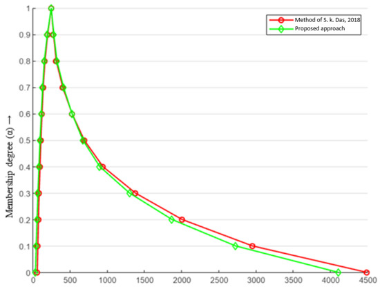
Figure 2. Comparison of optimal values of (M) for both the approaches. The red line presents the method proposed in [19].

5. Shortcomings of Existing Models and Motivation for the Proposed Approach

In real-world situations, we may come across FLFPPs having negative parameters. Since the approach used in [20] has some inconsistencies, there is a need to obtain an extended method that is applicable to FLFPPs with negative parameters as well. The motivation behind this article was to find a generalized method which provides a solution to an FLFPP with asymmetric fuzzy parameters which are unrestricted in sign.

The shortcomings of existing approaches along with the advantages of the proposed approach are listed below in Table 2.

Table 2. Comparison of proposed and existing approaches.

Approach	Shortcomings	Advantages of the Proposed Method over the Existing Approaches
1. Das and Mandal [11], Das et al. [12,19]	Fuzzy products and fractions are defined approximately.	$\alpha$-cut of fuzzy numbers and the decomposition theorem are used to define fuzzy arithmetic.
2. Borza et al. [16]	Variables are crisp.	Variables are TFNs.
3. Veeramani and Sumathi [17], Das et al. [19]	Applicable only when all the parameters are TFNs.	Applicable for any FLFPP with fuzzy numbers defined using $\alpha$-cut.
4. Mehra et al. [18]	Gives an $(\alpha ,\beta )$-acceptable optimal value for some fixed pair of $\alpha ,\beta \in (0.5,1]$, $\alpha ,\beta$ being cuts on the objective function and constraints, respectively.	Optimal values are obtained $\forall \alpha ,r\in (0,1]$, $\alpha ,r$ being cuts on the objective function and constraints, respectively.
5. Chinnadurai and Muthukumar [20]	Inconsistent when negative parameters are used.	Applicable even when negative parameters are involved.
6. Ebrahimnejad et al. [21]	Only applicable to problems with non-negative parameters.	Applicable irrespective of the nature of parameters involved.
7. Das [24]	The methodology lacks theoretical support.	Proposed technique is designed using fuzzy arithmetic and backed by various propositions.

6. Proposed $\alpha$-Cut-Based Method

To solve (M1), we use α as the satisfaction level on the objective function but for each constraint, different levels of satisfaction can be applied. For simplicity’s sake, the same satisfaction level r is used for all the constraints, throughout this paper.

For some fixed α and $r\in (0,1]$, after applying α-cut on the objective function and r-cut on all the constraints, we get the resulting model as:

$$\begin{array}{cc}\hfill & \mathit{Max}{\tilde{Z}}_{(\alpha ,r)}=\left[{\tilde{Z}}_{(\alpha ,r)}^L,{\tilde{Z}}_{(\alpha ,r)}^U\right]\hfill \\ \hfill & =\frac{{\left(\tilde{P}\left(\tilde{X}\right)\right)}_{\alpha }}{{\left(\tilde{Q}\left(\tilde{X}\right)\right)}_{\alpha }}\hfill \\ \hfill & {\displaystyle =\frac{{\displaystyle \left[{\displaystyle \sum _{j=1}^n{\left({\tilde{c}}_j\otimes {\tilde{x}}_j\right)}_{\alpha }^L+{\tilde{e}}_{\alpha }^L,\sum _{j=1}^n{\left(\widetilde{c_j}\otimes {\tilde{x}}_j\right)}_{\alpha }^U+{\tilde{e}}_{\alpha }^U}\right]}}{\left[{\displaystyle \sum _{j=1}^n{\left({\tilde{d}}_j\otimes {\tilde{x}}_j\right)}_{\alpha }^L+{\tilde{f}}_{\alpha }^L,\sum _{j=1}^n{\left({\tilde{d}}_j\otimes {\tilde{x}}_j\right)}_{\alpha }^U+{\tilde{f}}_{\alpha }^U}\right]}\mathrm{where}\sum _{j=1}^n{\left({\tilde{d}}_j\otimes {\tilde{x}}_j\right)}_{\alpha }^L+{\tilde{f}}_{\alpha }^L>0,}\hfill \\ \hfill & \mathrm{subject}\mathrm{to}\hfill \\ \hfill & {\displaystyle \sum _{j=1}^n\left[{\left({\tilde{a}}_{ij}\otimes {\tilde{x}}_j\right)}_r^L,{\left({\tilde{a}}_{ij}\otimes {\tilde{x}}_j\right)}_r^U\right]\le \left[{\left({\tilde{b}}_i{)}_r^L,({\tilde{b}}_i\right)}_r^U\right]\mathrm{for}i=1,2,\cdots ,m,}\hfill \\ \hfill & x_j\ge 0,{x_j}^{\prime }-x_j\ge 0,{x_j}^{″}-{x_j}^{\prime }\ge 0\mathrm{for}j=1,2,\cdots ,n.\hfill \end{array}$$

Since $S_1\ne \varnothing ,$ if an optimal solution $\tilde{X}$ exists, then by Proposition 2, $\tilde{X}\in S_1$. Hence, we need to solve the model for solutions in the set $S_1$ only. Therefore, to solve the model, we use the conditions of $S_1$, given by $\tilde{P}\left(\tilde{X}\right)⪰0$ and $\tilde{Q}\left(\tilde{X}\right)\succ 0$. This further implies that $\forall \alpha \in (0,1],0\le {\tilde{P}\left(\tilde{X}\right)}_{\alpha }^L\le {\tilde{P}\left(\tilde{X}\right)}_{\alpha }^U$ and $0<{\tilde{Q}\left(\tilde{X}\right)}_{\alpha }^L\le {\tilde{Q}\left(\tilde{X}\right)}_{\alpha }^U$. Using arithmetic operations for closed intervals, we obtain the following model:

$\left(FLFPP\right)\mathit{Max}\left[{\tilde{Z}}_{\alpha ,r}^L,{\tilde{Z}}_{\alpha ,r}^U\right]=\left[{\displaystyle \frac{{\displaystyle \sum _{j=1}^n{\left({\tilde{c}}_j\otimes {\tilde{x}}_j\right)}_{\alpha }^L+{\left(\tilde{e}\right)}_{\alpha }^L}}{{\displaystyle \sum _{j=1}^n{\left({\tilde{d}}_j\otimes {\tilde{x}}_j\right)}_{\alpha }^U+{\left(\tilde{f}\right)}_{\alpha }^U}},\frac{{\displaystyle \sum _{j=1}^n{\left({\tilde{c}}_j\otimes {\tilde{x}}_j\right)}_{\alpha }^U+{\left(\tilde{e}\right)}_{\alpha }^U}}{{\displaystyle \sum _{j=1}^n{\left({\tilde{d}}_j\otimes {\tilde{x}}_j\right)}_{\alpha }^L+{\left(\tilde{f}\right)}_{\alpha }^L}}}\right]$ where ${\displaystyle \sum _{j=1}^n{\left({\tilde{d}}_j\otimes {\tilde{x}}_j\right)}_{\alpha }^L+{\left(\tilde{f}\right)}_{\alpha }^L>0,}$

subject to

$${\displaystyle \sum _{j=1}^n{\left({\tilde{a}}_{ij}\otimes {\tilde{x}}_j\right)}_r^L\le ({\tilde{b}}_i{)}_r^L,}$$

$${\displaystyle \sum _{j=1}^n{\left({\tilde{a}}_{ij}\otimes {\tilde{x}}_j\right)}_r^U\le ({\tilde{b}}_i{)}_r^U\mathrm{for}i=1,2,\cdots ,m,}$$

$$x_j\ge 0,{x_j}^{\prime }-x_j\ge 0,{x_j}^{″}-{x_j}^{\prime }\ge 0\mathrm{for}j=1,2,\cdots ,n.$$

The above problem is then split into two separate problems, viz.,

$${\displaystyle \mathit{Lower}-\mathit{boundobjective}:\mathit{Max}{\tilde{Z}}_{\alpha ,r}^L=\frac{{\displaystyle \sum _{j=1}^n{({\tilde{c}}_j\otimes {\tilde{x}}_j)}_{\alpha }^L+{\left(\tilde{e}\right)}_{\alpha }^L}}{{\displaystyle \sum _{j=1}^n{({\tilde{d}}_j\otimes {\tilde{x}}_j)}_{\alpha }^U+{\left(\tilde{f}\right)}_{\alpha }^U}}\mathrm{where}{\displaystyle \sum _{j=1}^n{({\tilde{d}}_j\otimes {\tilde{x}}_j)}_{\alpha }^U+{\left(\tilde{f}\right)}_{\alpha }^U}>0,}$$

subject to all the constraints of (FLFPP).

$${\displaystyle \mathit{Upper}-\mathit{boundobjective}:\mathit{Max}{\tilde{Z}}_{\alpha ,r}^U=\frac{{\displaystyle \sum _{j=1}^n{({\tilde{c}}_j\otimes {\tilde{x}}_j)}_{\alpha }^U+{\left(\tilde{e}\right)}_{\alpha }^U}}{{\displaystyle \sum _{j=1}^n{({\tilde{d}}_j\otimes {\tilde{x}}_j)}_{\alpha }^L+{\left(\tilde{f}\right)}_{\alpha }^L}}\mathrm{where}\sum _{j=1}^n{({\tilde{d}}_j\otimes {\tilde{x}}_j)}_{\alpha }^L+{\left(\tilde{f}\right)}_{\alpha }^L>0,}$$

subject to all the constraints of (FLFPP).

The variables ${\tilde{x}}_j$ are considered to be non-negative TFNs, while there are no restrictions on the parameters ${\tilde{c}}_j,{\tilde{d}}_j\mathrm{and}{\tilde{a}}_{ij}\mathrm{for}i=1,2,\cdots ,m\mathrm{and}j=1,2,\cdots ,n.$ Therefore, after using Remark 2, both the bounds and the constraints are further reduced as follows:

Lower-bound objective:

$$\begin{array}{cc}\hfill \left(LB\right)& {\displaystyle \mathit{Max}{\tilde{Z}}_{\alpha ,r}^L=\frac{{\displaystyle \sum _{j=1}^n\min \left\{{\left({\tilde{c}}_j\right)}_{\alpha }^L{\left({\tilde{x}}_j\right)}_{\alpha }^L,{\left({\tilde{c}}_j\right)}_{\alpha }^L{\left({\tilde{x}}_j\right)}_{\alpha }^U\right\}+{\left(\tilde{e}\right)}_{\alpha }^L}}{{\displaystyle \sum _{j=1}^n\max \left\{{\left({\tilde{d}}_j\right)}_{\alpha }^U{\left({\tilde{x}}_j\right)}_{\alpha }^L,{\left({\tilde{d}}_j\right)}_{\alpha }^U{\left({\tilde{x}}_j\right)}_{\alpha }^U\right\}+{\left(\tilde{f}\right)}_{\alpha }^U}}}\hfill \end{array}$$

where

$${\displaystyle \sum _{j=1}^n\max \left\{{\left({\tilde{d}}_j\right)}_{\alpha }^U{\left({\tilde{x}}_j\right)}_{\alpha }^L,{\left({\tilde{d}}_j\right)}_{\alpha }^U{\left({\tilde{x}}_j\right)}_{\alpha }^U\right\}+{\left(\tilde{f}\right)}_{\alpha }^U}>0,$$

subject to

$${\displaystyle \sum _{j=1}^n\min \left\{{\left({\tilde{a}}_{ij}\right)}_r^L{\left({\tilde{x}}_j\right)}_r^L,{\left({\tilde{a}}_{ij}\right)}_r^L{\left({\tilde{x}}_j\right)}_r^U\right\}\le {\left({\tilde{b}}_i\right)}_r^L,}$$

$${\displaystyle \sum _{j=1}^n\max \left\{{\left({\tilde{a}}_{ij}\right)}_r^U{\left({\tilde{x}}_j\right)}_r^L,{\left({\tilde{a}}_{ij}\right)}_r^U{\left({\tilde{x}}_j\right)}_r^U\right\}\le {\left({\tilde{b}}_i\right)}_r^U\mathrm{for}i=1,2,\cdots ,m,}$$

$$x_j\ge 0,{x_j}^{\prime }-x_j\ge 0,{x_j}^{″}-{x_j}^{\prime }\ge 0\mathrm{for}j=1,2,\cdots ,n.$$

Upper-bound objective:

$${\displaystyle \left(UB\right)Max{\tilde{Z}}_{\alpha ,r}^U=\frac{{\displaystyle \sum _{j=1}^n\max \left\{{\left({\tilde{c}}_j\right)}_{\alpha }^U{\left({\tilde{x}}_j\right)}_{\alpha }^L,{\left({\tilde{c}}_j\right)}_{\alpha }^U{\left({\tilde{x}}_j\right)}_{\alpha }^U\right\}+{\left(\tilde{e}\right)}_{\alpha }^U}}{{\displaystyle \sum _{j=1}^n\min \left\{{\left({\tilde{d}}_j\right)}_{\alpha }^L{\left({\tilde{x}}_j\right)}_{\alpha }^L,{\left({\tilde{d}}_j\right)}_{\alpha }^L{\left({\tilde{x}}_j\right)}_{\alpha }^U\right\}+{\left(\tilde{f}\right)}_{\alpha }^L}}}$$

where

$${\displaystyle \sum _{j=1}^n\min \left\{{\left({\tilde{d}}_j\right)}_{\alpha }^L{\left({\tilde{x}}_j\right)}_{\alpha }^L,{\left({\tilde{d}}_j\right)}_{\alpha }^L{\left({\tilde{x}}_j\right)}_{\alpha }^U\right\}+{\left(\tilde{f}\right)}_{\alpha }^L}>0,$$

subject to all the constraints of the (LB).

Remark 4.

The membership function of the given objective function for some fixed value of $r\in (0,1]$ is obtained by plotting a graph between the intervals $[{\tilde{Z}}_{\alpha ,r}^L,{\tilde{Z}}_{\alpha ,r}^U]$ corresponding to $\alpha \in (0,1]$. The proposed method works for any FLFPP irrespective of the nature of the parameters.

7. Illustrative Examples

In this section, an example from the literature and a real-world application in the transportation sector, having unrestricted parameters, are worked out to illustrate the proposed method.

Example 1

([20]). Consider the following FLFPP:

$$\begin{array}{c}\hfill Maximize\tilde{Z}={\displaystyle \frac{(0,1,2)\otimes (x_1,x_1^{\prime },x_1^{″})\oplus (-2,-1,0)\otimes (x_2,x_2^{\prime },x_2^{″})\oplus (0,1,2)}{(0,1,2)\otimes (x_1,x_1^{\prime },x_1^{″})\oplus (0,1,2)\otimes (x_2,x_2^{\prime },x_2^{″})\oplus (1,2,3)}}\end{array}$$

subject to

$$\begin{array}{cc}\hfill & (0,1,2)\otimes (x_1,x_1^{\prime },x_1^{″})\oplus (0,1,2)\otimes (x_2,x_2^{\prime },x_2^{″})⪯(1,2,3),\hfill \\ \hfill & (0,1,2)\otimes (x_1,x_1^{\prime },x_1^{″})\oplus (-2,-1,0)\otimes (x_2,x_2^{\prime },x_2^{″})⪯(0,1,2),\hfill \\ \hfill & (x_1,x_1^{\prime },x_1^{″})⪰0,(x_2,x_2^{\prime },x_2^{″})⪰0.\hfill \end{array}$$

For some fixed values of $\alpha ,r\in (0,1]$, using the algorithm in Section 6, the lower-bound and upper-bound objectives of the problem are as follows:

Lower-bound objective:

$$\mathrm{(LB1)}\mathit{Max}{\tilde{Z}}_{\alpha ,r}^L=\frac{{\left({\tilde{c}}_1\right)}_{\alpha }^L{\left({\tilde{x}}_1\right)}_{\alpha }^L+{\left({\tilde{c}}_2\right)}_{\alpha }^L{\left({\tilde{x}}_2\right)}_{\alpha }^U+{\left(\tilde{e}\right)}_{\alpha }^L}{{\left({\tilde{d}}_1\right)}_{\alpha }^U{\left({\tilde{x}}_1\right)}_{\alpha }^U+{\left({\tilde{d}}_2\right)}_{\alpha }^U{\left({\tilde{x}}_2\right)}_{\alpha }^U+{\left(\tilde{f}\right)}_{\alpha }^U}$$

subject to

$$\begin{array}{cc}\hfill & {\left({\tilde{a}}_{11}\right)}_r^L{\left({\tilde{x}}_1\right)}_r^L+{\left({\tilde{a}}_{12}\right)}_r^L{\left({\tilde{x}}_2\right)}_r^L\le {\left({\tilde{b}}_1\right)}_r^L,\hfill \\ \hfill & {\left({\tilde{a}}_{21}\right)}_r^L{\left({\tilde{x}}_1\right)}_r^L+{\left({\tilde{a}}_{22}\right)}_r^L{\left({\tilde{x}}_2\right)}_r^U\le {\left({\tilde{b}}_2\right)}_r^L,\hfill \\ \hfill & {\left({\tilde{a}}_{11}\right)}_r^U{\left({\tilde{x}}_1\right)}_r^U+{\left({\tilde{a}}_{12}\right)}_r^U{\left({\tilde{x}}_2\right)}_r^U\le {\left({\tilde{b}}_1\right)}_r^U,\hfill \\ \hfill & {\left({\tilde{a}}_{21}\right)}_r^U{\left({\tilde{x}}_1\right)}_r^U+{\left({\tilde{a}}_{22}\right)}_r^U{\left({\tilde{x}}_2\right)}_r^L\le {\left({\tilde{b}}_2\right)}_r^U,\hfill \\ \hfill & x_i\ge 0,x_i^{\prime }-x_i\ge 0,x_i^{″}-x_i^{\prime }\ge 0\mathrm{for}i=1,2.\hfill \\ \hfill & \left(\mathrm{As}{\tilde{c}}_2\mathrm{and}{\tilde{a}}_{22}\mathrm{are}\mathrm{negative}.\right)\hfill \end{array}$$

Upper-bound objective:

$$\begin{gathered} \mathrm{(UB1)}Max{\tilde{Z}}_{\alpha ,r}^U=\frac{{\left({\tilde{c}}_1\right)}_{\alpha }^U{\left({\tilde{x}}_1\right)}_{\alpha }^U+{\left({\tilde{c}}_2\right)}_{\alpha }^U{\left({\tilde{x}}_2\right)}_{\alpha }^L+{\left(\tilde{e}\right)}_{\alpha }^U}{{\left({\tilde{d}}_1\right)}_{\alpha }^L{\left({\tilde{x}}_1\right)}_{\alpha }^L+{\left({\tilde{d}}_2\right)}_{\alpha }^L{\left({\tilde{x}}_2\right)}_{\alpha }^L+{\left(\tilde{f}\right)}_{\alpha }^L} \\ \mathrm{subject} \mathrm{to} \mathrm{all} \mathrm{the} \mathrm{constraints} \mathrm{of} (\mathrm{LB}1). \end{gathered}$$

Substituting values of all $\alpha ,r$-cut, the bounds are rewritten as:

Lower-bound objective:

$$\begin{array}{cc}\hfill (\mathrm{LB}1-1)& {\displaystyle \mathit{Max}{\tilde{Z}}_{\alpha ,r}^L=\frac{\left(\alpha \right)(x_1+(x_1^{\prime }-x_1)\alpha )+(-2+\alpha )(x_2^{″}-(x_2^{″}-x_2^{\prime })\alpha )+\left(\alpha \right)}{(2-\alpha )(x_1^{″}-(x_1^{″}-x_1^{\prime })\alpha )+(2-\alpha )(x_2^{″}-(x_2^{″}-x_2^{\prime })\alpha )+(3-\alpha )}}\hfill \end{array}$$

subject to

$$\begin{array}{cc}\hfill & \left(r\right)(x_1+(x_1^{\prime }-x_1)r)+\left(r\right)(x_2+(x_2^{\prime }-x_2)r)\le (1+r),\hfill \\ \hfill & \left(r\right)(x_1+(x_1^{\prime }-x_1)r)+(-2+r)(x_2^{″}-(x_2^{″}-x_2^{\prime })r)\le r,\hfill \\ \hfill & (2-r)(x_1^{″}-(x_1^{″}-x_1^{\prime })r)+(2-r)(x_2^{″}-(x_2^{″}-x_2^{\prime })r)\le (3-r),\hfill \\ \hfill & (2-r)(x_1^{″}-(x_1^{″}-x_1^{\prime })r)+(-r)(x_2+(x_2^{\prime }-x_2)r)\le (2-r),\hfill \\ \hfill & x_i\ge 0,x_i^{\prime }-x_i\ge 0,x_i^{″}-x_i^{\prime }\ge 0\mathrm{for}i=1,2.\hfill \end{array}$$

Upper-bound objective:

${\displaystyle (\mathrm{UB}1-1)Max{\tilde{Z}}_{\alpha ,r}^U=\frac{(2-\alpha )(x_1^{″}-(x_1^{″}-x_1^{\prime })\alpha )+(-\alpha )(x_2+(x_2^{\prime }-x_2)\alpha )+(2-\alpha )}{\left(\alpha \right)(x_1+(x_1^{\prime }-x_1)\alpha )+\left(\alpha \right)(x_2+(x_2^{\prime }-x_2)\alpha )+(1+\alpha )}}$ subject to all the constraints of (LB1-1).

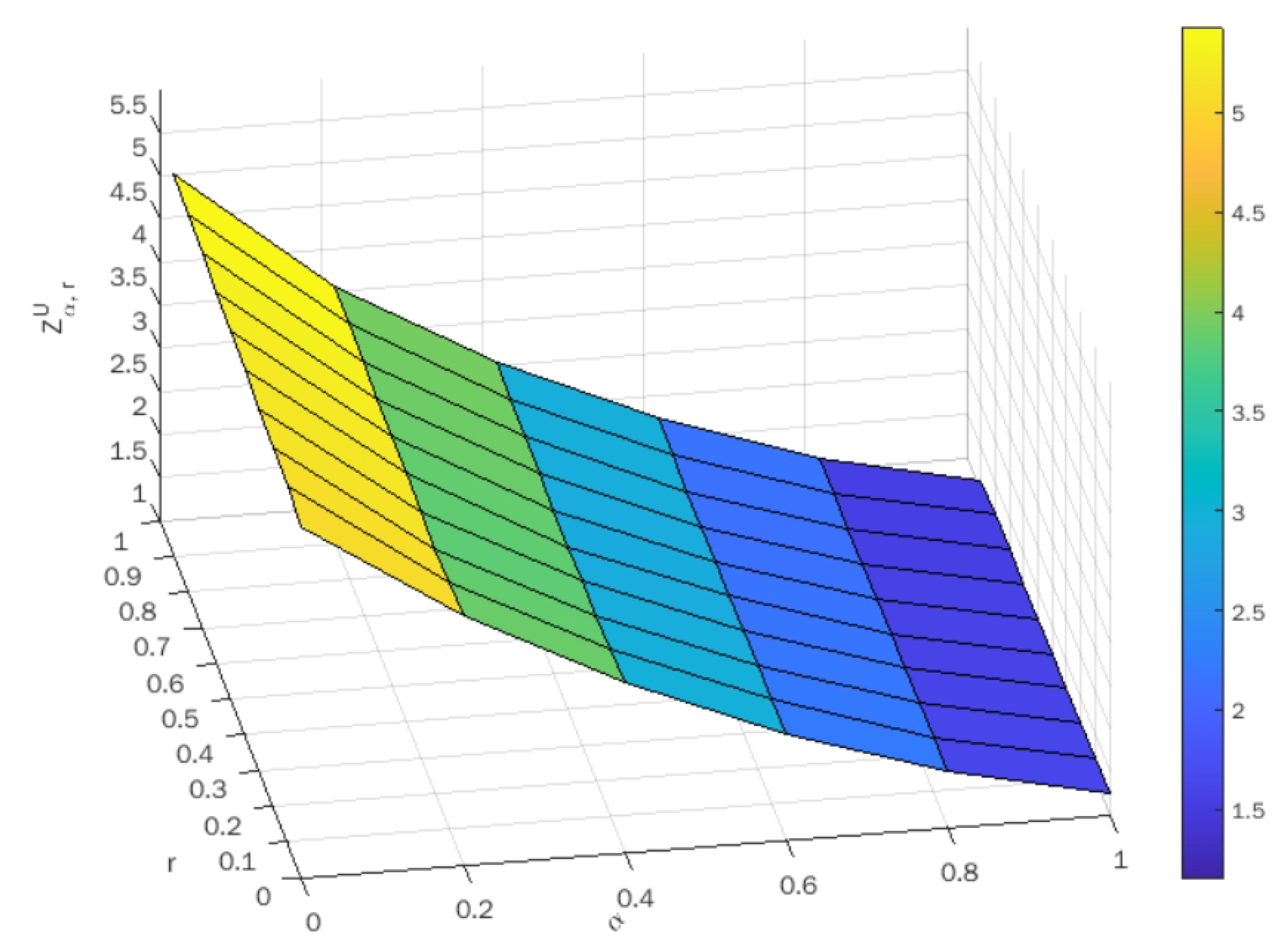
Upon taking different values of $\alpha ,r\in (0,1]$, the optimal value of both the lower-bound and upper-bound objectives are indicated in Table 3 and Table 4, respectively. Using these tables, the surface plots of objective values against $(\alpha ,r)$ are shown in Figure 3 and Figure 4 for the lower-bound and upper-bound objectives, respectively.

Table 3. Optimal values of the objective function ${\tilde{Z}}_{\alpha ,r}^L$.

$\mathit{r}\setminus \mathit{\alpha }$	0	0.2	0.4	0.6	0.8	1
0	0	0.087	0.1905	0.3158	0.4706	0.6667
0.1	0	0.087	0.1905	0.3158	0.4706	0.6667
0.2	0	0.087	0.1905	0.3158	0.4706	0.6667
0.3	0	0.087	0.1905	0.3158	0.4706	0.6667
0.4	0	0.087	0.1905	0.3158	0.4706	0.6667
0.5	0	0.087	0.1905	0.3158	0.4706	0.6667
0.6	0	0.087	0.1905	0.3158	0.4706	0.6667
0.7	0	0.087	0.1905	0.3158	0.4706	0.6667
0.8	0	0.087	0.1905	0.3158	0.4706	0.6667
0.9	0	0.087	0.1905	0.3158	0.4706	0.6667
0.99 ≈ 1	0	0.087	0.1905	0.3158	0.4706	0.6667

Table 4. Optimal values of the objective function ${\tilde{Z}}_{\alpha ,r}^U$.

$\mathit{r}\setminus \mathit{\alpha }$	0	0.2	0.4	0.6	0.8	1
0	4.0000	2.9032	2.0513	1.4286	0.9836	0.6667
0.1	4.2807	2.9032	2.0513	1.4286	0.9836	0.6667
0.2	4.6389	3.0000	2.0513	1.4286	0.9836	0.6667
0.3	5.1092	3.2143	2.1225	1.4286	0.9836	0.6667
0.4	5.7500	3.5279	2.2857	1.4583	0.9836	0.6667
0.5	6.6667	4.0333	2.5140	1.5750	0.9836	0.6667
0.6	8.0714	4.8279	2.8571	1.7500	1.0000	0.6667
0.7	10.4615	6.2081	3.6152	2.0417	1.1111	0.6667
0.8	15.3333	9.0569	5.1813	2.6820	1.3333	0.6667
0.9	30.1818	17.7983	9.9863	5.0157	2.0000	0.6667
0.99 ≈ 1	300.028	177.031	97.4943	47.4623	17.2443	0.6667

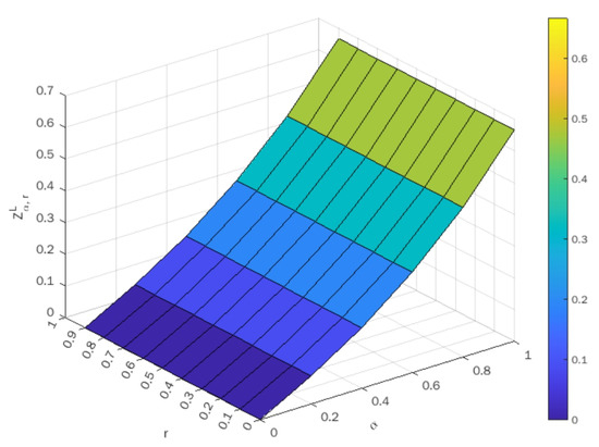
Figure 3. Surface plot of optimal values corresponding to ${\tilde{Z}}_{\alpha ,r}^L$.

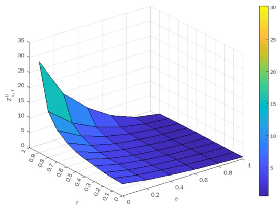
Figure 4. Surface plot of optimal values corresponding to ${\tilde{Z}}_{\alpha ,r}^U$.

Figure 5 represents the membership function of objective function $\tilde{Z}$ when particular values are considered for $r=0.1,0.5$ and $0.7.$

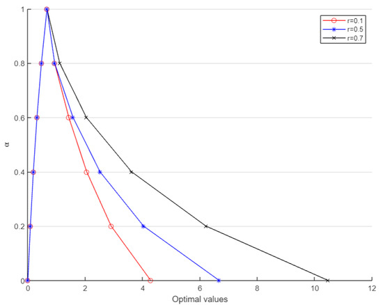
Figure 5. Membership function of the objective function $\tilde{Z}$ (Example 1) for $r=0.1,0.5\mathrm{and}0.7$.

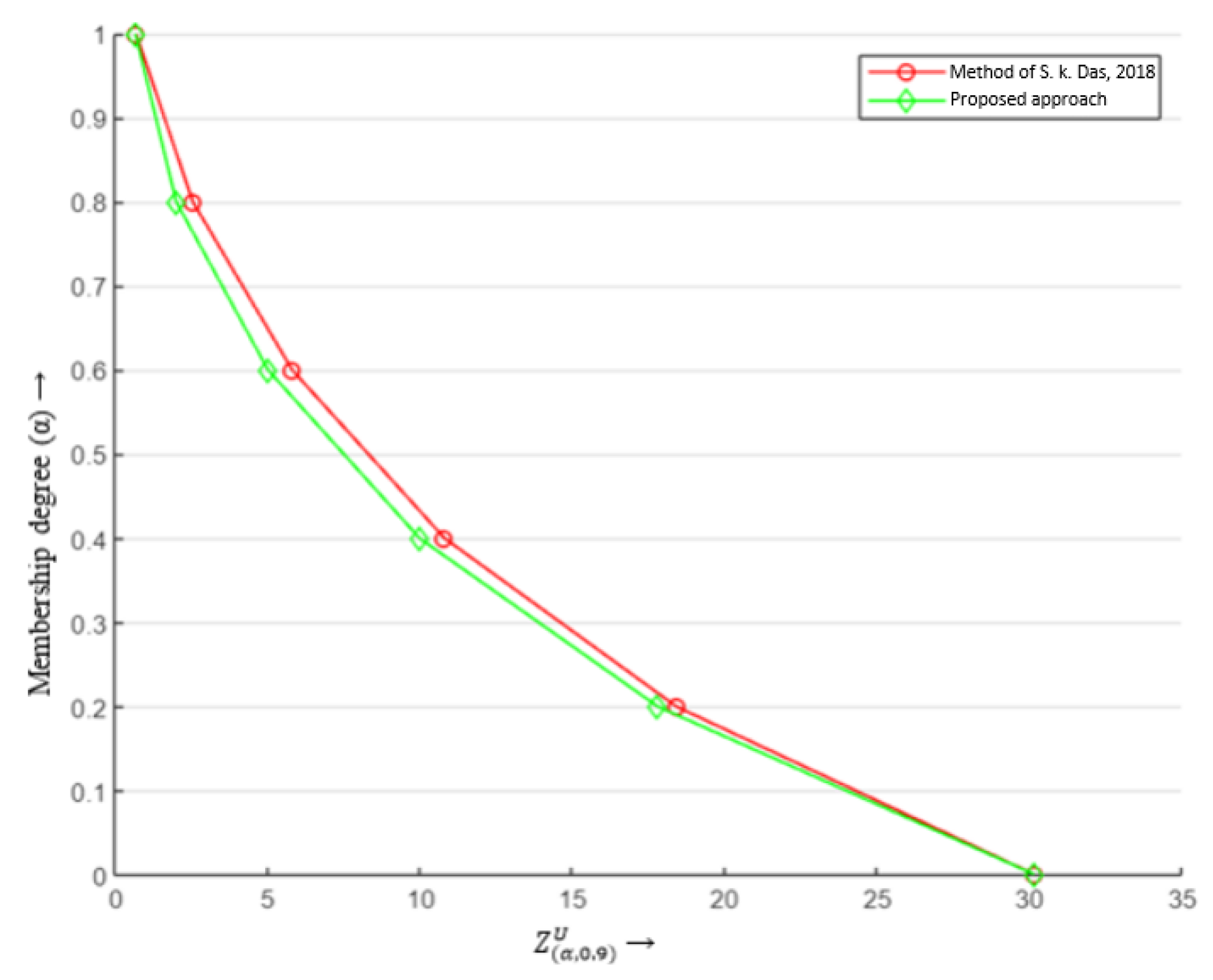
Observation 2: In Table 5, the optimal values of the lower- and upper-bound objectives are compared using $r=0.9$ and different values of $\alpha$, using the approach in [20] and the proposed approach. The lower-bound objective values are identical for all $\alpha$ but the upper-bound objective values exhibit the fallacy in Chinnadurai and Muthukumar’s [20] approach. This shows that the optimal values obtained using the method in [20] are misleading and different from the actual ones.

Table 5. $\left[Z_{(\alpha ,0.9)}^L,Z_{(\alpha ,0.9)}^U\right]$ using the approach in [20] vs. proposed method.

$\mathit{\alpha }(\mathit{r}=0.9)$	Approach in [20]	Proposed Method
0	$[0,30.182]$	$[0,30.181]$
$0.2$	$[0.087,18.409]$	$[0.087,17.798]$
$0.4$	$[0.191,10.8052]$	$[0.191,9.986]$
$0.6$	$[0.316,5.807]$	$[0.316,5.0157]$
$0.8$	$[0.471,2.545]$	$[0.471,2.00]$
0.99 #x2248;x 2248;1	$[0.679,0.679]$	$[0.667,0.667]$

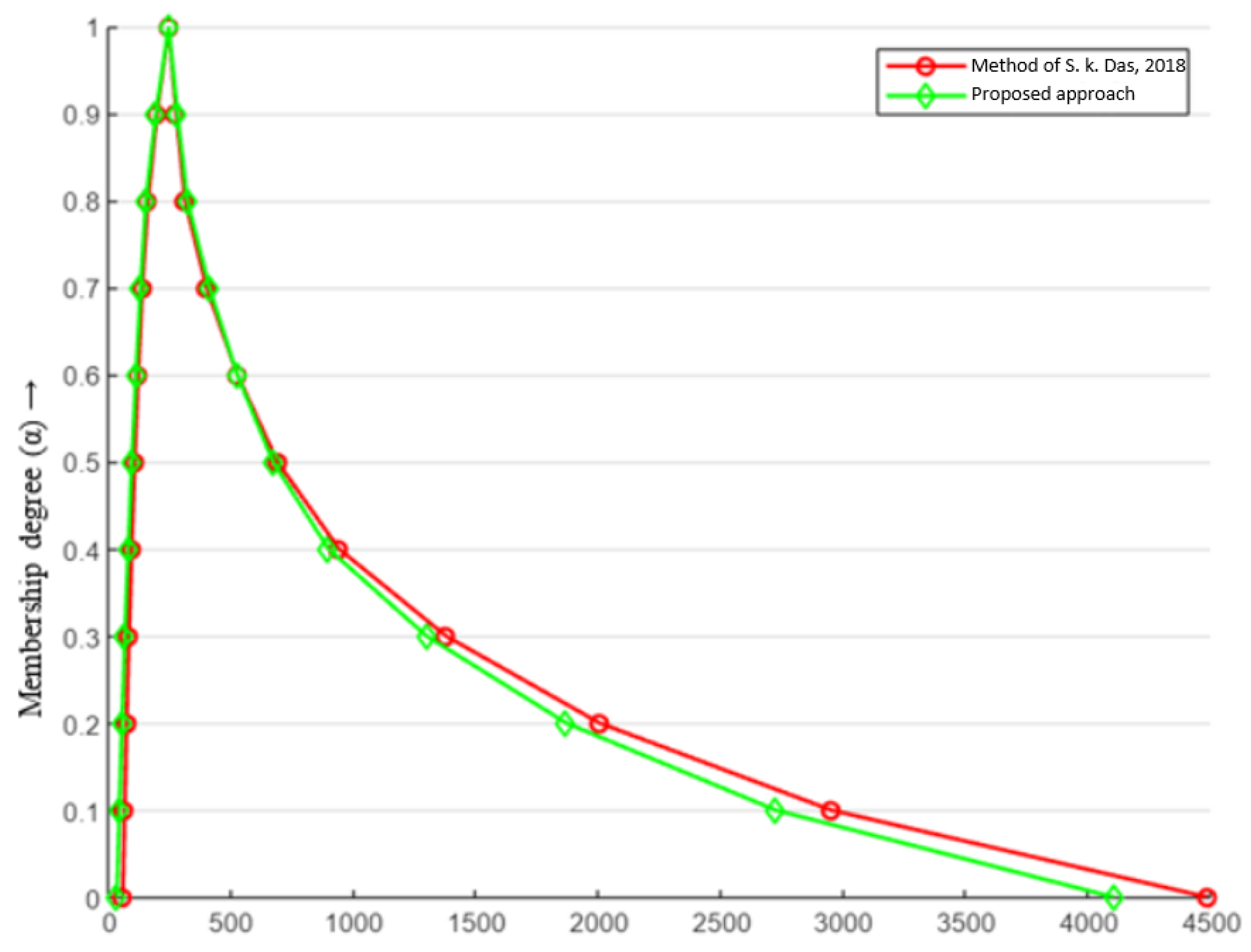
Figure 6 shows the contrast between the optimal values for the upper-bound objective evaluated using both approaches.

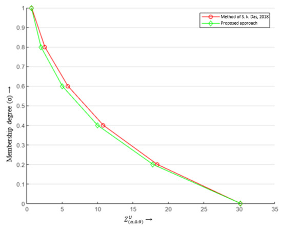
Figure 6. Comparison of $Z_{(\alpha ,0.9)}^U$ values. The red line presents the method proposed in [19].

Example 2.

Application in transportation sector.

A leading textile company has a well-established network of stores and factory outlets. Due to industrialisation and urbanisation, the demand for their goods at three factory outlets $O_1,O_2\mathrm{and}{O}_3$ is expected to increase. As the future requirement is imprecise and uncertain, TFNs are used to represent the foreseen requirements at these outlets as given in Table 6. To meet these requirements, the company decides to establish two new storages $S_1\mathrm{and}{S}_2$. The storage capacities are estimated and are indicated in Table 7. Table 8 and Table 9 give the presumed profit and cost of transport per unit of product from the ith store to the jth outlet.

Table 6. Requirement at the outlets.

Outlet	${\mathit{O}}_1$	${\mathit{O}}_2$	${\mathit{O}}_3$
Requirement	$\widetilde{R_1}=(7,9,10)$	$\widetilde{R_2}=(6,7,8)$	$\widetilde{R_3}=(10,12,13)$

Table 7. Capacity of the stores.

Store	${\mathit{S}}_1$	${\mathit{S}}_2$
Store capacity	$\widetilde{S_1}=(9,10,11)$	$\widetilde{S_2}=(14,18,20)$

Table 8. Profit ${\tilde{c}}_{ij}$ per unit product sold from the outlets (in thousands).

Store∖Outlets	${\mathit{O}}_1$	${\mathit{O}}_2$	${\mathit{O}}_3$
$S_1$	$\$(0,10,20)$	$\$(-1,2,5)$	$\$(5,6,7)$
$S_2$	$\$(4,4.5,5)$	$\$(1,6,12)$	$\$(-10,0,5)$

Table 9. Transportation cost ${\tilde{d}}_{ij}$ (in thousands).

Store∖Outlets	${\mathit{O}}_1$	${\mathit{O}}_2$	${\mathit{O}}_3$
$S_1$	$\$(3,6,9)$	$\$(9,10,11)$	$\$(0,2,5)$
$S_2$	$\$(4.5,5,5.5)$	$\$(6,8,14)$	$\$(1.5,1.5,3)$

The company aims to obtain the maximum value of expected profit–cost ratio (PCR) for transporting their goods between these selected storage facilities and the outlets with a view to seek future prospects.

Let ${\tilde{x}}_{ij}=(x_{ij}^l,x_{ij},x_{ij}^u)$ be the units of products transported between the ith store and the jth outlet. The proposed technique is applied to forecast the maximum PCR value. The fuzzy linear fractional programming model framed using Table 6, Table 7, Table 8 and Table 9 is as follows:

$$\mathrm{Maximize}\tilde{Z}={\displaystyle \frac{\left\{\begin{array}{c}(0,10,20)\otimes (x_{11}^l,x_{11},x_{11}^u)\oplus (-1,2,5)\otimes (x_{12}^l,x_{12},x_{12}^u)\hfill \\ \oplus (5,6,7)\otimes (x_{13}^l,x_{13},x_{13}^u)\oplus (4,4.5,5)\otimes (x_{21}^l,x_{21},x_{21}^u)\\ \hfill \oplus (1,6,12)\otimes (x_{22}^l,x_{22},x_{22}^u)\oplus (-10,0,5)\otimes (x_{23}^l,x_{23},x_{23}^u)\end{array}\right\}}{\left\{\begin{array}{c}(3,6,9)\otimes (x_{11}^l,x_{11},x_{11}^u)\oplus (9,10,11)\otimes (x_{12}^l,x_{12},x_{12}^u)\hfill \\ \oplus (0,2,5)\otimes (x_{13}^l,x_{13},x_{13}^u)\oplus (4.5,5,5)\otimes (x_{21}^l,x_{21},x_{21}^u)\\ \hfill \oplus (6,8,14)\otimes (x_{22}^l,x_{22},x_{22}^u)\oplus (1.5,1.5,3)\otimes (x_{23}^l,x_{23},x_{23}^u)\end{array}\right\}}}$$

subject to $\hspace{1em}\hspace{1em}\hspace{1em} (x_{11}^l,x_{11},x_{11}^u)\oplus (x_{12}^l,x_{12},x_{12}^u)\oplus (x_{13}^l,x_{13},x_{13}^u)⪯(9,10,11),$

$\hspace{1em}\hspace{1em}\hspace{1em}\hspace{1em}\hspace{1em}\hspace{1em}(x_{21}^l,x_{21},x_{21}^u)\oplus (x_{22}^l,x_{22},x_{22}^u)\oplus (x_{23}^l,x_{23},x_{23}^u)⪯(14,18,20),$

$\hspace{1em}\hspace{1em}\hspace{1em}\hspace{1em}\hspace{1em}\hspace{1em}(x_{11}^l,x_{11},x_{11}^u)\oplus (x_{21}^l,x_{21},x_{21}^u)⪰(7,9,10),$

$\hspace{1em}\hspace{1em}\hspace{1em}\hspace{1em}\hspace{1em}\hspace{1em}(x_{12}^l,x_{12},x_{12}^u)\oplus (x_{22}^l,x_{22},x_{22}^u)⪰(6,7,8),$

$\hspace{1em}\hspace{1em}\hspace{1em}\hspace{1em}\hspace{1em}\hspace{1em}(x_{13}^l,x_{13},x_{13}^u)\oplus (x_{23}^l,x_{23},x_{23}^u)⪰(10,12,13),$

$\hspace{1em}\hspace{1em}\hspace{1em}\hspace{1em}\hspace{1em}\hspace{1em}{x}_{ij}^l\ge 0,x_{ij}-x_{ij}^l\ge 0,x_{ij}^u-x_{ij}\ge 0$ where $i=1,2\mathrm{and}j=1,2,3.$

The decision-maker can fix the satisfaction levels $\alpha ,r\in (0,1]$, for the objective function and constraints, respectively. Using the algorithm in Section 6, the lower and upper bounds of the problem are obtained as follows:

Lower-bound objective:

$$\begin{array}{cc}\hfill \left(LB2\right)& \mathit{Max}{\tilde{Z}}_{\alpha ,r}^L=\left\{\begin{array}{c}{\displaystyle \frac{\left\{\begin{array}{c}{\left({\tilde{c}}_{11}\right)}_{\alpha }^L{\left({\tilde{x}}_{11}\right)}_{\alpha }^L+{\left({\tilde{c}}_{12}\right)}_{\alpha }^L{\left({\tilde{x}}_{12}\right)}_{\alpha }^L+{\left({\tilde{c}}_{13}\right)}_{\alpha }^L{\left({\tilde{x}}_{13}\right)}_{\alpha }^L\hfill \\ \hfill +{\left({\tilde{c}}_{21}\right)}_{\alpha }^L{\left({\tilde{x}}_{21}\right)}_{\alpha }^L+{\left({\tilde{c}}_{22}\right)}_{\alpha }^L{\left({\tilde{x}}_{22}\right)}_{\alpha }^L+{\left({\tilde{c}}_{23}\right)}_{\alpha }^L{\left({\tilde{x}}_{23}\right)}_{\alpha }^U\end{array}\right\}}{\left\{\begin{array}{c}{\left({\tilde{d}}_{{}_{11}}\right)}_{\alpha }^U{\left({\tilde{x}}_{11}\right)}_{\alpha }^U+{\left({\tilde{d}}_{{}_{12}}\right)}_{\alpha }^U{\left({\tilde{x}}_{12}\right)}_{\alpha }^U+{\left({\tilde{d}}_{{}_{13}}\right)}_{\alpha }^U{\left({\tilde{x}}_{13}\right)}_{\alpha }^U\hfill \\ \hfill +{\left({\tilde{d}}_{{}_{21}}\right)}_{\alpha }^U{\left({\tilde{x}}_{21}\right)}_{\alpha }^U+{\left({\tilde{d}}_{{}_{22}}\right)}_{\alpha }^U{\left({\tilde{x}}_{22}\right)}_{\alpha }^U+{\left({\tilde{d}}_{{}_{23}}\right)}_{\alpha }^U{\left({\tilde{x}}_{23}\right)}_{\alpha }^U\end{array}\right\}}},\alpha \ge \frac{1}{3},\hfill \\ \\ {\displaystyle \frac{\left\{\begin{array}{c}{\left({\tilde{c}}_{11}\right)}_{\alpha }^L{\left({\tilde{x}}_{11}\right)}_{\alpha }^L+{\left({\tilde{c}}_{12}\right)}_{\alpha }^L{\left({\tilde{x}}_{12}\right)}_{\alpha }^U+{\left({\tilde{c}}_{13}\right)}_{\alpha }^L{\left({\tilde{x}}_{13}\right)}_{\alpha }^L\hfill \\ \hfill +{\left({\tilde{c}}_{21}\right)}_{\alpha }^L{\left({\tilde{x}}_{21}\right)}_{\alpha }^L+{\left({\tilde{c}}_{22}\right)}_{\alpha }^L{\left({\tilde{x}}_{22}\right)}_{\alpha }^L+{\left({\tilde{c}}_{23}\right)}_{\alpha }^L{\left({\tilde{x}}_{23}\right)}_{\alpha }^U\end{array}\right\}}{\left\{\begin{array}{c}{\left({\tilde{d}}_{{}_{11}}\right)}_{\alpha }^U{\left({\tilde{x}}_{11}\right)}_{\alpha }^U+{\left({\tilde{d}}_{{}_{12}}\right)}_{\alpha }^U{\left({\tilde{x}}_{12}\right)}_{\alpha }^U+{\left({\tilde{d}}_{{}_{13}}\right)}_{\alpha }^U{\left({\tilde{x}}_{13}\right)}_{\alpha }^U\hfill \\ \hfill +{\left({\tilde{d}}_{{}_{21}}\right)}_{\alpha }^U{\left({\tilde{x}}_{21}\right)}_{\alpha }^U+{\left({\tilde{d}}_{{}_{22}}\right)}_{\alpha }^U{\left({\tilde{x}}_{22}\right)}_{\alpha }^U+{\left({\tilde{d}}_{{}_{23}}\right)}_{\alpha }^U{\left({\tilde{x}}_{23}\right)}_{\alpha }^U\end{array}\right\}}},\alpha <\frac{1}{3}\hfill \end{array}\right.\hfill \end{array}$$

subject to

$$\begin{array}{cc}\hfill & {\displaystyle \sum _{j=1}^3{\left({\tilde{x}}_{ij}\right)}_r^L\le {\left(\widetilde{S_i}\right)}_r^L,}\hfill \\ \hfill & {\displaystyle \sum _{j=1}^3{\left({\tilde{x}}_{ij}\right)}_r^U\le {\left(\widetilde{S_i}\right)}_r^U\mathrm{for}i=1,2,}\hfill \\ \hfill & {\displaystyle \sum _{i=1}^2{\left({\tilde{x}}_{ij}\right)}_r^L\ge {\left(\widetilde{R_j}\right)}_r^L,}\hfill \\ \hfill & {\displaystyle \sum _{i=1}^2{\left({\tilde{x}}_{ij}\right)}_r^U\ge {\left(\widetilde{R_j}\right)}_r^U\mathrm{for}j=1,2,3,}\hfill \\ \hfill & x_{ij}^l\ge 0,x_{ij}-x_{ij}^l\ge 0,x_{ij}^r-x_{ij}\ge 0\mathrm{where}i=1,2\mathrm{and}j=1,2,3.\hfill \end{array}$$

(As ${\left({\tilde{c}}_{12}\right)}_{\alpha }^L$ and ${\left({\tilde{c}}_{23}\right)}_{\alpha }^L$ are negative for some values of $\alpha \in (0,1]$.)

Upper-bound objective:

$\left(UB2\right)Max{\tilde{Z}}_{\alpha ,r}^U={\displaystyle \frac{\left\{\begin{array}{c}{\left({\tilde{c}}_{11}\right)}_{\alpha }^U{\left({\tilde{x}}_{11}\right)}_{\alpha }^U+{\left({\tilde{c}}_{12}\right)}_{\alpha }^U{\left({\tilde{x}}_{12}\right)}_{\alpha }^U+{\left({\tilde{c}}_{13}\right)}_{\alpha }^U{\left({\tilde{x}}_{13}\right)}_{\alpha }^U\\ +{\left({\tilde{c}}_{21}\right)}_{\alpha }^U{\left({\tilde{x}}_{21}\right)}_{\alpha }^U+{\left({\tilde{c}}_{22}\right)}_{\alpha }^U{\left({\tilde{x}}_{22}\right)}_{\alpha }^U+{\left({\tilde{c}}_{23}\right)}_{\alpha }^U{\left({\tilde{x}}_{23}\right)}_{\alpha }^U\end{array}\right\}}{\left\{\begin{array}{c}{\left({\tilde{d}}_{{}_{11}}\right)}_{\alpha }^L{\left({\tilde{x}}_{11}\right)}_{\alpha }^L+{\left({\tilde{d}}_{{}_{12}}\right)}_{\alpha }^L{\left({\tilde{x}}_{12}\right)}_{\alpha }^L+{\left({\tilde{d}}_{{}_{13}}\right)}_{\alpha }^L{\left({\tilde{x}}_{13}\right)}_{\alpha }^L\\ +{\left({\tilde{d}}_{{}_{21}}\right)}_{\alpha }^L{\left({\tilde{x}}_{21}\right)}_{\alpha }^L+{\left({\tilde{d}}_{{}_{22}}\right)}_{\alpha }^L{\left({\tilde{x}}_{22}\right)}_{\alpha }^L+{\left({\tilde{d}}_{{}_{23}}\right)}_{\alpha }^L{\left({\tilde{x}}_{23}\right)}_{\alpha }^L\end{array}\right\}}}$ subject to all the constraints of (LB2).

Substituting all $\alpha ,r$-cut values, we get the bounds as:

Lower-bound objective:

$$(\mathrm{L}\mathrm{B}2-1){\tilde{Z}}_{\alpha ,r}^L=\left\{\begin{array}{c}{\displaystyle \frac{\left\{\begin{array}{c}\left(10\alpha \right)\left(x_{11}^l+\alpha (x_{11}-x_{11}^l)\right)+(3\alpha -1)\left(x_{12}^l+\alpha (x_{12}-x_{12}^l)\right)+\hfill \\ (5+\alpha )\left(x_{13}^l+\alpha (x_{13}-x_{13}^l)\right)+(4+0.5\alpha )\left(x_{21}^l+\alpha (x_{21}-x_{21}^l)\right)+\\ (5\alpha +1)\left(x_{22}^l+\alpha (x_{22}-x_{22}^l)\right)+(10\alpha -10)\left(x_{23}^u-\alpha (x_{23}^u-x_{23})\right)\end{array}\right\}}{\left\{\begin{array}{c}(9-3\alpha )\left(x_{11}^u-\alpha (x_{11}^u-x_{11})\right)+(11-\alpha )\left(x_{12}^u-\alpha (x_{12}^u-x_{12})\right)+\\ (5-3\alpha )\left(x_{13}^u-\alpha (x_{13}^u-x_{13})\right)+\left(5\right)\left(x_{21}^u-\alpha (x_{21}^u-x_{21})\right)+\\ (14-6\alpha )\left(x_{22}^u-\alpha (x_{22}^u-x_{22})\right)+(3-1.5\alpha )\left(x_{23}^u-\alpha (x_{23}^u-x_{23})\right)\end{array}\right\}}},\alpha \ge \frac{1}{3},\hfill \\ {\displaystyle \frac{\left\{\begin{array}{c}\left(10\alpha \right)\left(x_{11}^l+\alpha (x_{11}-x_{11}^l)\right)+(3\alpha -1)\left(x_{12}^u-\alpha (x_{12}^u-x_{12})\right)+\hfill \\ (5+\alpha )\left(x_{13}^l+\alpha (x_{13}-x_{13}^l)\right)+(4+0.5\alpha )\left(x_{21}^l+\alpha (x_{21}-x_{21}^l)\right)+\\ (5\alpha +1)\left(x_{22}^l+\alpha (x_{22}-x_{22}^l)\right)+(10\alpha -10)\left(x_{23}^u-\alpha (x_{23}^u-x_{23})\right)\end{array}\right\}}{\left\{\begin{array}{c}(9-3\alpha )\left(x_{11}^u-\alpha (x_{11}^u-x_{11})\right)+(11-\alpha )\left(x_{12}^u-\alpha (x_{12}^u-x_{12})\right)+\\ (5-3\alpha )\left(x_{13}^u-\alpha (x_{13}^u-x_{13})\right)+\left(5\right)\left(x_{21}^u-\alpha (x_{21}^u-x_{21})\right)+\\ (14-6\alpha )\left(x_{22}^u-\alpha (x_{22}^u-x_{22})\right)+(3-1.5\alpha )\left(x_{23}^u-\alpha (x_{23}^u-x_{23})\right)\end{array}\right\}}},\alpha <\frac{1}{3}\hfill \end{array}\right.$$

subject to

$$\begin{array}{cc}\hfill & \left(x_{11}^l+r(x_{11}-x_{11}^l)\right)+\left(x_{12}^l+r(x_{12}-x_{12}^l)\right)+\left(x_{13}^l+r(x_{13}-x_{13}^l)\right)\le 9+r,\hfill \\ \hfill & \left(x_{21}^l+r(x_{21}-x_{21}^l)\right)+\left(x_{22}^l+r(x_{22}-x_{22}^l)\right)+\left(x_{23}^l+r(x_{23}-x_{23}^l)\right)\le 14+4r,\hfill \\ \hfill & \left(x_{11}^u-r(x_{11}^u-x_{11})\right)+\left(x_{12}^u-r(x_{12}^u-x_{12})\right)+\left(x_{13}^u-r(x_{13}^u-x_{13})\right)\le 11-r,\hfill \\ \hfill & \left(x_{21}^u-r(x_{21}^u-x_{21})\right)+\left(x_{22}^u-r(x_{22}^u-x_{22})\right)+\left(x_{23}^u-r(x_{23}^u-x_{23})\right)\le 20-2r,\hfill \\ \hfill & \left(x_{11}^l+r(x_{11}-x_{11}^l)\right)+\left(x_{21}^l+r(x_{21}-x_{21}^l)\right)\ge 7+2r,\hfill \\ \hfill & \left(x_{12}^l+r(x_{12}-x_{12}^l)\right)+\left(x_{22}^l+r(x_{22}-x_{22}^l)\right)\ge 6+r,\hfill \\ \hfill & (x_{13}^l+r(x_{13}-x_{13}^l))+\left(x_{23}^l+r(x_{23}-x_{23}^l)\right)\ge 10+2r,\hfill \\ \hfill & \left(x_{11}^u-r(x_{11}^u-x_{11})\right)+\left(x_{21}^u-r(x_{21}^u-x_{21})\right)\ge 10-r,\hfill \\ \hfill & \left(x_{12}^u-r(x_{12}^u-x_{12})\right)+\left(x_{22}^u-r(x_{22}^u-x_{22})\right)\ge 8-r,\hfill \\ \hfill & \left(x_{13}^u-r(x_{13}^u-x_{13})\right)+\left(x_{23}^u-r(x_{23}^u-x_{23})\right)\ge 13-r,\hfill \\ \hfill & x_{ij}^l\ge 0,(x_{ij}-x_{ij}^l)\ge 0,(x_{ij}^u-x_{ij})\ge 0\mathrm{where}i=1,2\mathrm{and}j=1,2,3.\hfill \end{array}$$

Upper-bound objective:

$$(UB-1)Max{\tilde{Z}}_{\alpha ,r}^L={\displaystyle \frac{\left\{\begin{array}{c}(20-10\alpha )\left(x_{11}^u-\alpha (x_{11}^u-x_{11})\right)+(5-3\alpha )\left(x_{12}^u-\alpha (x_{12}^u-x_{12})\right)+\\ (7-\alpha )\left(x_{13}^u-\alpha (x_{13}^u-x_{13})\right)+(5-0.5\alpha )\left(x_{21}^u-\alpha (x_{21}^u-x_{21})\right)+\\ (12-6\alpha )\left(x_{22}^u-\alpha (x_{22}^u-x_{22})\right)+(5-5\alpha )\left(x_{23}^u-\alpha (x_{23}^u-x_{23})\right)\end{array}\right\}}{\left\{\begin{array}{c}(3+3\alpha )\left(x_{11}^l+\alpha (x_{11}-x_{11}^l)\right)+(9+\alpha )\left(x_{12}^l+\alpha (x_{12}-x_{12}^l)\right)+\\ \left(2\alpha \right)\left(x_{13}^l+\alpha (x_{13}-x_{13}^l)\right)+(4.5+0.5\alpha )\left(x_{21}^l+\alpha (x_{21}-x_{21}^l)\right)+\\ (6+2\alpha )\left(x_{22}^l+\alpha (x_{22}-x_{22}^l)\right)+\left(1.5\right)\left(x_{23}^l+\alpha (x_{23}-x_{23}^l)\right)\end{array}\right\}}}$$

subject to all the constraints of (LB2-1).

The optimal value of lower-bound and upper-bound objectives corresponding to various values of $\alpha ,r\in (0,1]$ are indicated in Table 10 and Table 11, respectively. The surface plots of objective values against $(\alpha ,r)$ are shown in Figure 7 and Figure 8 for lower-bound and upper-bound objectives, respectively.

Table 10. Optimal values of the objective function ${\tilde{Z}}_{\alpha ,r}^L$.

$\mathit{r}\setminus \mathit{\alpha }$	0	0.2	0.4	0.6	0.8	1
0	0.2646	0.3872	0.5345	0.7136	0.9392	1.2535
0.1	0.2698	0.3783	0.5259	0.7054	0.9305	1.2416
0.2	0.2751	0.3696	0.5174	0.6973	0.9220	1.2300
0.3	0.2803	0.375	0.5090	0.6893	0.9138	1.2188
0.4	0.2856	0.3803	0.5006	0.6813	0.9058	1.2079
0.5	0.2908	0.3857	0.5059	0.6733	0.8980	1.1974
0.6	0.2961	0.391	0.5112	0.6654	0.8904	1.1872
0.7	0.3013	0.3963	0.5165	0.6705	0.8830	1.1773
0.8	0.3065	0.4016	0.5219	0.6757	0.8758	1.1676
0.9	0.3117	0.4069	0.5271	0.6808	0.8805	1.1583
0.99 ≈ 1	0.3668	0.4723	0.5964	0.7448	0.9252	1.1492

Table 11. Optimal values of the objective function ${\tilde{Z}}_{\alpha ,r}^U$.

$\mathit{r}\setminus \mathit{\alpha }$	0	0.2	0.4	0.6	0.8	1
0	5.0725	3.8951	2.9670	2.2298	1.6412	1.2535
0.1	5.1101	3.8636	2.9452	2.2141	1.6290	1.2416
0.2	5.1483	3.8329	2.9240	2.1987	1.6170	1.2300
0.3	5.1870	3.8540	2.9033	2.1836	1.6052	1.2188
0.4	5.2262	3.8750	2.8831	2.1688	1.5937	1.2079
0.5	5.2659	3.8961	2.8979	2.1544	1.5824	1.1974
0.6	5.3062	3.9171	2.9126	2.1402	1.5716	1.1872
0.7	5.3470	3.9381	2.9273	2.1505	1.5603	1.1773
0.8	5.3884	3.9599	2.9420	2.1608	1.5496	1.1676
0.9	5.4303	3.9862	2.9566	2.1710	1.5566	1.1583
0.99 ≈ 1	5.3044	3.9771	2.9816	2.2897	1.7139	1.1492

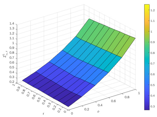
Figure 7. Surface plot of optimal values corresponding to ${\tilde{Z}}_{\alpha ,r}^L$.

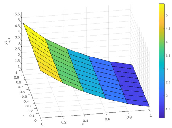
Figure 8. Surface plot of optimal values corresponding to ${\tilde{Z}}_{\alpha ,r}^U$.

The choice of satisfaction level where $\alpha =r=1$ corresponds to the crisp case and the maximum PCR is predicted to be 1.149. In realistic scenarios, such crisp values lack much significance as uncertainty is involved. Thus, for some fixed satisfaction levels of the objective and constraints, respectively, a range of PCR values are evaluated and examined. For example, if the decision-maker selects $r=0.5$ as the satisfaction level of constraints and $\alpha =0.8$ for the objective function, then the anticipated PCR range is $[0.898,1.5824]$. This gives a better picture to the company for looking into future prospects.

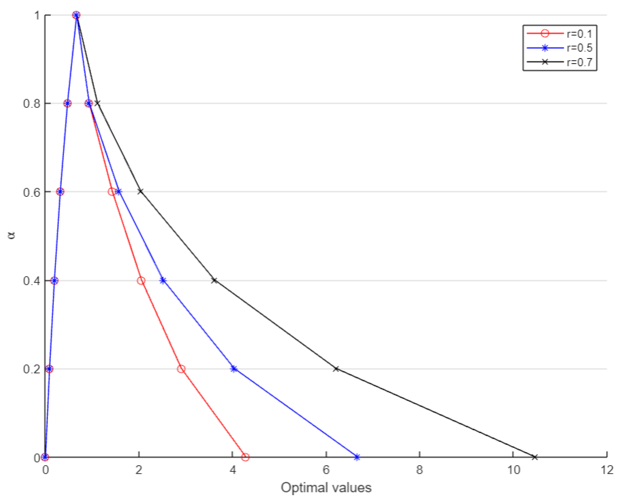
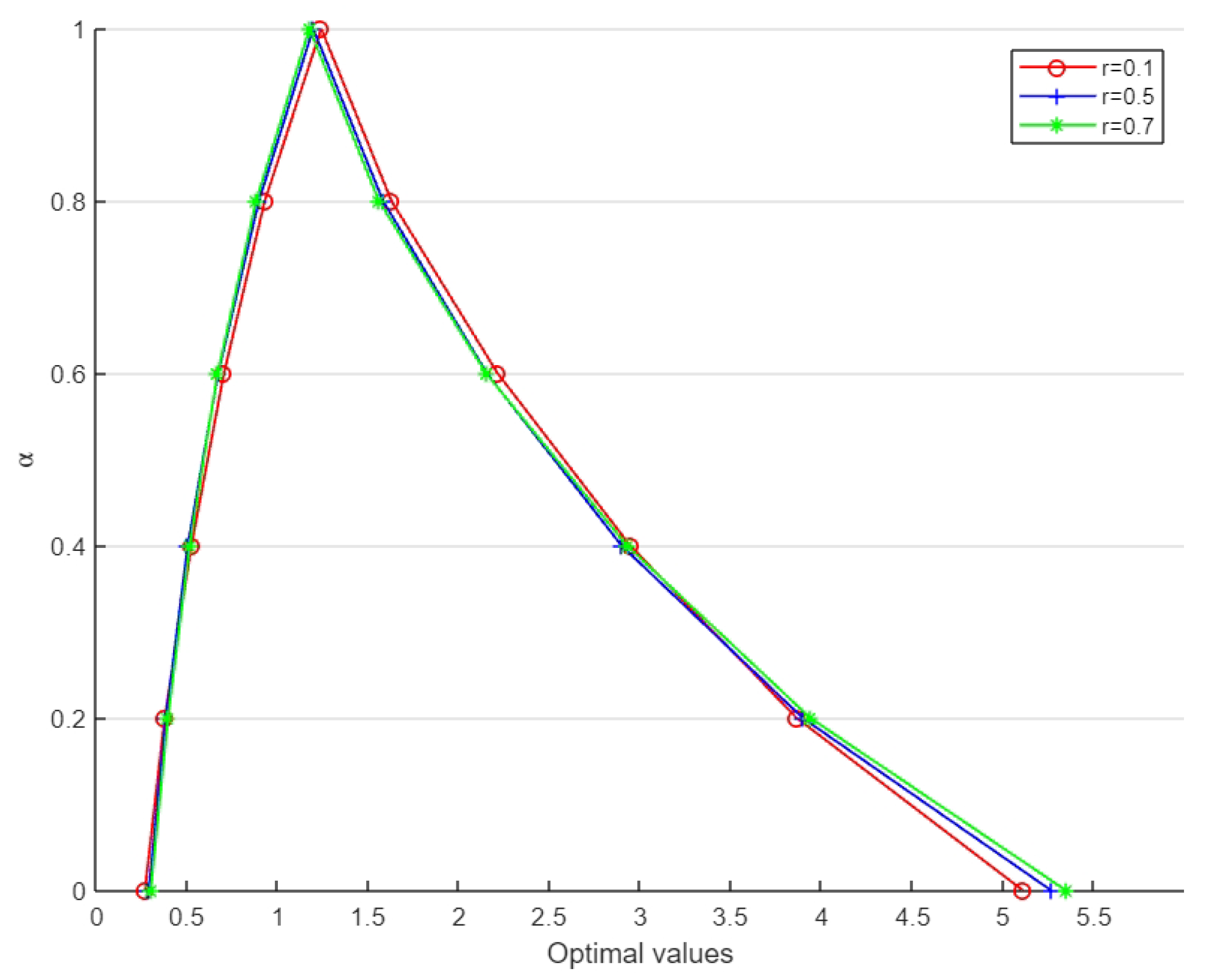
Moreover, for a fixed satisfaction level of the constraints, the membership function of foreseen PCR can be obtained using different $\alpha$ values. For some given values of r, i.e., $r=0.1,0.5$ and $0.7$, the corresponding membership function is shown in Figure 9.

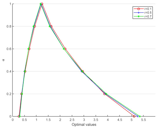
Figure 9. Membership function of the objective function $\tilde{Z}$ (Example 2) for $r=0.1,0.5\mathrm{and}0.7$.

8. Results and Discussion

In Example 1, we solved an FLFPP with unrestricted parameters and later compared the results with the approach in [20]. For example, when we fixed $r=0.9$ and $\alpha =0.4$, the $\left[Z_{(0.4,0.9)}^L,Z_{(0.4,0.9)}^U\right]$ value obtained using [20]’s approach was [0.191, 10.8052] whereas using the proposed approach, we obtained $\left[Z_{(0.4,0.9)}^L,Z_{(0.4,0.9)}^U\right]=$ [0.191, 9.986]. This contrast in $Z_{(\alpha ,0.9)}^U$ values for both approaches could be observed for the rest of $\alpha$ values as well, as indicated in Table 5. Thereafter, Example 2 modelled a real-life transportation problem as an FLFPP to forecast the maximum PCR based on the given data. The decision-maker could predict a range of PCR values using Table 10 and Table 11; for instance, when $\alpha =0.4$ and $r=0.8$ were selected then the predicted PCR range was [0.5219, 2.9420]. Finally, it could be noticed from Figure 5 and Figure 9 that the membership function corresponding to different $\alpha$ and r values gave rise to TFNs. This validated the proposed $\alpha$-cut-based approach.

9. Conclusions and Future Scope

In this article, the limitation of Chinnadurai and Muthukumar’s [20] approach was indicated by a counterexample and then the method was extended and generalized for FLFPPs having parameters that are unrestricted in sign. The method was demonstrated using $(\alpha ,r)$-cuts by fixing some value of $\alpha$ and $r\in (0,1]$. The FLFPP was reduced to a crisp biobjective problem that comprised the lower- and upper-bound objectives, which were solved to obtain a numerical solution. Various values of $\alpha$ and $r\in (0,1]$ were fixed and the corresponding solutions were obtained. These solutions were then used to plot the membership function of the initial objective function corresponding to fixed values of r. Examples 1 and 2 were solved to illustrate the proposed approach.

In future work, the same model can be extended for the class of problems where $S_1=\varnothing$. For simplicity, we considered parameters and variables to be TFNs. For further studies, FLFPPs having parameters as intuitionistic fuzzy or type-2 fuzzy numbers can be investigated. A wide variety of fractional programming problems are nonlinear in nature and may have multiple objective functions or criteria associated with them. The proposed approach can be amalgamated with goal/fuzzy programming or the TOPSIS method to tackle the problem.

References

- Charnes, A.; Cooper, W.W. Programming with linear fractional functionals. Nav. Res. Logist. Q. 1962, 9, 181–186. [Google Scholar] [CrossRef]
- Tantawy, S.F. A new procedure for solving linear fractional programming problems. Math. Comput. Model. 2009, 48, 969–973. [Google Scholar] [CrossRef]
- Chadha, S.S.; Chadha, V. Linear fractional programming and duality. Cent. Eur. J. Oper. Res. 2007, 15, 119–125. [Google Scholar] [CrossRef]
- Rizk-Allah, R.M.; Hassanien, A.E.; Bhattacharyya, S. Chaotic crow search algorithm for fractional optimization problems. Appl. Soft Comput. 2018, 71, 1161–1175. [Google Scholar] [CrossRef]
- Sharma, S.C.; Bansal, A. A integer solution of fractional programming problem. Gen. Math. Notes 2011, 4, 1–9. [Google Scholar]
- Pandey, P.; Punnen, A.P. A simplex algorithm for piecewise-linear fractional programming problems. Eur. J. Oper. Res. 2007, 178, 343–358. [Google Scholar] [CrossRef]
- Zadeh, L.A. Fuzzy sets. Inform. Control 1965, 8, 338–353. [Google Scholar] [CrossRef]
- Hladík, M. Generalized linear fractional programming under interval uncertainty. Eur. J. Oper. Res. 2010, 205, 42–46. [Google Scholar] [CrossRef]
- Borza, M.; Rambely, A.S.; Saraj, M. Solving linear fractional programming problems with interval coefficients in the objective function. A new approach. Appl. Math. Sci. 2012, 6, 3443–3452. [Google Scholar]
- Pandian, P.; Jayalakshmi, M. On solving linear fractional programming problems. Mod. Appl. Sci. 2013, 7, 90. [Google Scholar]
- Das, S.K.; Mandal, T. A MOLFP method for solving linear fractional programming under fuzzy environment. Int. J. Ind. Eng. 2017, 6, 202–213. [Google Scholar]
- Das, S.K.; Edalatpanah, S.A.; Mandal, T. Application of linear fractional programming problem with fuzzy nature in industry sector. Filomat 2020, 34, 5073–5084. [Google Scholar] [CrossRef]
- Sharma, M.K.; Dhiman, N.; Mishra, V.N.; Rosales, H.G.; Dhaka, A.; Nandal, A.; Mishra, L.N. A fuzzy optimization technique for multi-objective aspirational level fractional transportation problem. Symmetry 2021, 13, 1465. [Google Scholar] [CrossRef]
- Dutta, D.; Rao, J.R.; Tiwari, R.N. Sensitivity analysis in fuzzy linear fractional programming problem. Fuzzy Sets Syst. 1992, 48, 211–216. [Google Scholar] [CrossRef]
- Dutta, D.; Rao, J.R.; Tiwari, R.N. Effect of tolerance in fuzzy linear fractional programming. Fuzzy Sets Syst. 1993, 55, 133–142. [Google Scholar] [CrossRef]
- Borza, M.; Rambely, A.S. An approach based on alpha-cut and max-min technique to linear fractional programming with fuzzy coefficients. Iran. J. Fuzzy Syst. 2022, 19, 153–168. [Google Scholar]
- Veeramani, C.; Sumathi, M. Fuzzy mathematical programming approach for solving fuzzy linear fractional programming problem. RAIRO-Oper. Res. 2014, 48, 109–122. [Google Scholar] [CrossRef]
- Mehra, A.; Chandra, S.; Bector, C.R. Acceptable optimality in linear fractional programming with fuzzy coefficients. Fuzzy Optim. Decis. Mak. 2007, 6, 5–16. [Google Scholar] [CrossRef]
- Das, S.K.; Edalatpanah, S.A.; Mandal, T. A proposed model for solving fuzzy linear fractional programming problem: Numerical Point of View. J. Comput. Sci. 2018, 25, 367–375. [Google Scholar] [CrossRef]
- Chinnadurai, V.; Muthukumar, S. Solving the linear fractional programming problem in a fuzzy environment: Numerical approach. Appl. Math. Model. 2016, 40, 6148–6164. [Google Scholar] [CrossRef]
- Ebrahimnejad, A.; Ghomi, S.J.; Mirhosseini-Alizamini, S.M. A revisit of numerical approach for solving linear fractional programming problem in a fuzzy environment. Appl. Math. Model. 2018, 57, 459–473. [Google Scholar] [CrossRef]
- Klir, G.; Yuan, B. Fuzzy Sets and Fuzzy Logic; Prentice Hall: Hoboken, NJ, USA, 1995; Volume 4, pp. 1–12. [Google Scholar]
- Gomathi, S.V.; Jayalakshmi, M. One’s Fixing Method for a Distinct Symmetric Fuzzy Assignment Model. Symmetry 2022, 14, 2056. [Google Scholar] [CrossRef]
- Das, S.K. An approach to optimize the cost of transportation problem based on triangular fuzzy programming problem. Complex Intell. Syst. 2022, 8, 687–699. [Google Scholar] [CrossRef]
Disclaimer/Publisher’s Note: The statements, opinions and data contained in all publications are solely those of the individual author(s) and contributor(s) and not of MDPI and/or the editor(s). MDPI and/or the editor(s) disclaim responsibility for any injury to people or property resulting from any ideas, methods, instructions or products referred to in the content. |
© 2023 by the authors. Licensee MDPI, Basel, Switzerland. This article is an open access article distributed under the terms and conditions of the Creative Commons Attribution (CC BY) license (https://creativecommons.org/licenses/by/4.0/).