Article

Non-Trivial Band Topology Criteria for Magneto-Spin–Orbit Graphene

by
Alexander V. Eryzhenkov
*,
Artem V. Tarasov
,
Alexander M. Shikin
* and
Artem G. Rybkin
Department of Physics, Saint Petersburg State University, 198504 Saint Petersburg, Russia
*
Authors to whom correspondence should be addressed.
Symmetry 2023, 15(2), 516; https://doi.org/10.3390/sym15020516
Submission received: 31 December 2022 / Revised: 23 January 2023 / Accepted: 7 February 2023 / Published: 15 February 2023
(This article belongs to the Special Issue Topological Quantum Materials and Applications)

Abstract

:
Band structure and topology of magneto-spin–orbit graphene is investigated using the proposed tight-binding model that incorporates both Rashba and sublattice-resolved collinear exchange couplings in a generic ferrimagnetic (FIM) setting for in-plane and out-of-plane magnetization directions. The resulting band structures were analyzed for possibilities to extract the strengths of exchange and Rashba couplings from experimental spin-resolved ARPES measurements of the valley gaps and π -state spin-splittings. It was shown that the topologically trivial in-plane FIM situation admits simple expressions for these quantities, whereas the out-of-plane FIM, which admits a nontrivial band topology, is harder to analyze. The obtained topological phase diagrams for the out-of-plane FIM case show that the anomalous Hall conductance is quite stable with respect to the antiferromagnetic (AFM) interaction, which tends to interfere with the QAHE phase; moreover, the topological phase transition has a rather smooth character with respect to the AFM coupling strength.

1. Introduction

Two-dimensional material study is an active field of research in solid-state physics due to numerous practically interesting properties of such materials. For example, transition metal dichalcogenides [1,2,3], black phosphorus [4] and other materials [5] are already studied extensively while the search for other two-dimensional topological materials continues [6].
The most notable example of a two-dimensional material is graphene, the nonmagnetic carbon allotrope. Its honeycomb geometry with two equivalent sublattices allows two valleys with a special kind of linear band dispersion (the Dirac cone), which defines excellent electronic [7], optic [8] and spin transport properties of graphene [9,10], including long spin relaxation times [11]. These may also serve as a good prerequisite for graphene-based spintronic devices [12,13,14,15] but only if some external sources of spin–orbit coupling and magnetism are provided since the intrinsic spin–orbit coupling is negligible [16]. A common route to achieve that goal is to utilize the proximity effect by placing graphene onto a high-Z or magnetic substrate, respectively, to generate sufficiently large Rashba spin–orbit [17,18,19,20,21,22,23,24,25,26] or exchange couplings [27,28,29,30,31,32] to exploit the spin degree of freedom of the Dirac electrons.
A promising approach that combines these magnetic and spin–orbit environments was laid out in a number of papers [24,25,26,33] where the graphene overlayer on top of magnetic materials such as Co or Ni was intercalated with Au to yield a quasifreestanding graphene monolayer on top of Au/Ni or Au/Co complex surface alloys containing triangular misfit loops [34]. The band and spin structure of these systems was characterized using spin- and angle-resolved photoemission spectroscopy (spin-ARPES) to conclude that a significant (>50 meV) Rashba spin–orbit coupling is induced on graphene, which itself has a quasifreestanding character (the Dirac cone is present). Scanning tunnel microscopy (STM) results allowed to additionally conclude that the graphene overlayer is almost flat in these systems. Another unusual common experimental observation contained in these papers is the spin-splitting valley asymmetry, which is not allowed for pure graphene/Rashba systems, thus suggesting an interplay between the Rashba coupling and the in-plane substrate magnetism; even the term “magneto-spin–orbit graphene” was coined to reflect these essential features.
Although the in-plane magnetization does not allow observing a long-sought quantum anomalous Hall effect (QAHE) in graphene systems [35,36], one may expect that similar systems but with out-of-plane magnetization may be engineered where the QAHE is possible. To accomplish this task, one would need a clear picture of the physics behind the magneto-spin–orbit graphene to decide whether a given candidate system may or may not exhibit the QAHE. Several attempts to investigate the essential physics were made using density functional theory (DFT) calculations; however, even the most realistic ones [26,37,38,39] where the large superstructure period was taken into account could not naturally reproduce such large Rashba spin-splittings using the ab initio unit cell optimization procedure. The corresponding spin-splitting magnitude either occurs to be too small or is quantitatively reproduced but with artificial graphene-substrate distance shrinkage [25]. This particular issue of DFT calculations with such systems remains unresolved to this day.
Nevertheless, the DFT calculations in [26] successfully reproduced the structural properties (misfit loops and the quasifreestanding character of graphene) of the graphene/Au/Co system and even suggested uniform graphene ferrimagnetism as a cause of the unusually large experimental band gap in an almost flat graphene overlayer (here, uniform means that the magnetic moments are periodic with 1 × 1 graphene cell period, whereas the calculated supercell size is 9 × 9 ). This partial success of DFT raises the question of whether the underlying magneto-spin–orbit graphene physics may be revealed at the level of simple models. The system geometry (large superstructure period and graphene flatness) confirmed by STM allows one to exclude various staggered sublattice potentials originating from different sublattice-dependent bonding environments. Another favorable consequence of this geometry together with the quasifreestanding graphene character is “smearing out” interactions between carbon atoms and substrate to yield an effective uniform picture that may be expected to be captured with relative simplicity.
This work suggests a tight-binding model that incorporates both Rashba spin–orbit coupling and uniform collinear sublattice magnetism and is expected to yield useful results on the whole class of systems described above. Although a large number of graphene tight-binding models involving various kinds of interactions is already known in the literature [40,41,42,43,44,45,46,47,48,49], these models either do not include ferrimagnetism and Rashba interaction simultaneously or have additional terms such as intrinsic spin–orbit coupling or other staggered sublattice potentials. In either case, essential correlations between a tight-binding model and experimental data was not sufficiently covered for mixed Rashba–magnetism environments typical for magneto-spin–orbit graphene systems.
An attempt is made in this work to close this gap; the authors also propose a method that allows an experimentalist to use some measurement procedures to decide which tight-binding parameters describe the experimental spin-resolved spectra satisfactorily (or at least to deduce proper initial conditions for a subsequent numerical optimization in complex cases). Since the number of observable quantities in a spin-resolved ARPES experiment is rather limited, the simplicity of the presented model is considered as an acceptable compromise (of course, within the model applicability). If the model parameters are properly assessed, then out-of-plane magnetized candidate systems for QAHE implementation may be determined using this method; the corresponding topological phase diagrams are included in this paper to serve this purpose.

2. Model Hamiltonian

The considered tight-binding model is formulated as
H = d r Ψ p 2 2 m + α ( r ) [ s × p ] z + U ( r , m ^ ) Ψ
where the terms are described in order of writing:
  • The kinetic energy that is evaluated to account only for the principal (nearest-neighbor) hopping;
  • The Rashba spin–orbit term reflecting the interaction between graphene and a high-Z substrate;
  • The collinear sublattice magnetization term (the magnetization direction is m ^ ).
The intrinsic spin–orbit term is not included because its coupling constant for pristine graphene is ≈ 0.01 meV [16]; such a weak term cannot break a topological order if the latter manifests due to the Rashba–exchange coupling mechanism [50].
The field operators in (1) are expanded as
Ψ ( r ) = R τ { A , B } σ { , } c R ; τ σ ϕ ( r r τ R ) χ σ , Ψ ( r ) = R τ σ c R ; τ σ ϕ * ( r r τ R ) χ σ ,
where c and c are annihilation and creation operators, r τ are vectors from the cell origin to the carbon atoms of the τ sublattice, ϕ ( r ) is a graphene real-space 2 p z -like basis function with presumed orthonormality, i. e., ϕ ( r r τ ) | ϕ ( r r τ ) = δ τ τ , and χ σ is a corresponding 2 × 1 column spinor. The summation over translation vectors R is to be performed over a crystal that consists of N unit cells linked by periodic boundary conditions.
After integration and Fourier transformation, the reciprocal space matrix Hamiltonian for collinear magnetizations along the vector m ^ in the { A , A , B , B } basis becomes
h ( k ) = 1 2 U m A ( s · m ^ ) t f ( k ) + R t f * ( k ) + R 1 2 U m B ( s · m ^ ) = u A ( s · m ^ ) ε e i ϑ + R ε e i ϑ + R u B ( s · m ^ )
where ε k = t | f ( k ) | , u A , B = 1 2 U m A , B and R = λ R 3 d ( s · rot f ) . All prefactors (t, λ R and U) are real-valued coupling constants, quantities m A and m B denote the corresponding sublattice magnetizations (either sign is allowed) and f ( k ) is the graphene geometric factor
f ( k ) = e i k d 1 + e i k d 2 + e i k d 3 | f ( k ) | e i ϑ ( k ) , rot f ( k ) = grad f ( k ) × e z = [ e x k y e y k x ] f ( k )
where d i are the nearest-neighbor hopping vectors from A to B sublattices, all of length d (see Figure A1 in Appendix A for coordinate system orientation). Another pair of variables denoting the magnetization state of the sublattices is also used further, “mean ferromagnetic energy” u FM = ( u A + u B ) / 2 and “mean antiferromagnetic energy” u AFM = ( u A u B ) / 2 .

3. Results

This section reveals some relations between the model parameters and experimental observables, which may be extracted from spin-resolved ARPES data. Two major ARPES scanning directions are often used when graphene is considered: either the Γ K M (the “along- Γ K ”) path or its orthogonal counterpart passing through the K or K points (the “ortho- Γ K ” path). In this work, only the first is explicitly presented using figures and tables, but all necessary conclusions for any other scanning path may be drawn using the provided generic equations.
In order to establish the problem framework, some trivial known results regarding graphene under only either exchange or Rashba interactions are summarized in Figure 1 (see Appendix B for their detailed presentation). Figure 1a shows the slope of the pristine graphene band dispersion, which may be used to determine the principal hopping integral t. Figure 1b depicts two completely spin-polarized and spin-split Dirac cones if graphene is subject to a uniform FM exchange field of the form u FM τ 0 s z . Figure 1c,d joined together show the K Γ K band dispersion of graphene only under the Rashba coupling of strength λ R . A spin-splitting sign convention is chosen such that the splitting Δ is evaluated as Δ = E VB E VB , and this value is marked on these figures; this convention is used further in the text.

3.1. In-Plane Magnetized Graphene with Rashba Interaction

General case of in-plane ferrimagnetic graphene with the magnetization direction vector m ^ and angle α = arg ( m x + i m y ) accompanied by the Rashba spin–orbit coupling is given by the Hamiltonian
h ( k ) = 0 u A e i α ε e i ϑ i λ R K u A e i α 0 i λ R K ε e i ϑ ε e i ϑ i λ R K 0 u B e i α i λ R K ε e i ϑ u B e i α 0
which is reduced to a μ -Hamiltonian (A7) in Appendix C (provided k is far enough from the Dirac points):
h μ ( k + ν K ) = μ ε u FM ( s · m ^ ) + μ λ R 2 ( s · [ e z × k ^ ] ) .
The energy splitting between the bands has a magnitude of
Δ ϕ k = λ R 2 + 4 u FM 2 + 4 μ λ R u FM sin ( ϕ k α )
which depends only on a mutual alignment of k ^ and m ^ , not on a valley index per se. The spin texture vector lies in-plane:
n μ ( k ) Δ ϕ 1 ( μ λ R [ e z × k ^ ] 2 u FM m ^ ) .
All situations of in-plane ferrimagnetism with Rashba coupling may be divided into four classes with respect to two experimentally discernible alternatives: whether | u FM | > | u AFM | or not (zero/nonzero gap value is the deciding factor) and whether 2 | u FM | > | λ R | or not (the spin splitting sign inversion absence/presence is the deciding factor). This classification is summarized in Table 1 with some examples of band diagrams on the corresponding figures.
The first illustrated case is the FM-dominated FIM with the magnetization vector m ^ = e y (first row of Figure 2), where λ R > 2 u FM > 2 u AFM > 0 . Figure 2a,b show the y-spin texture of bands plotted along the orthogonal x-direction where the absence of Rashba-like spin-splitting inversion (as in Figure 1c,d) is evident. The spin ordering is thus classified as persistent in Table 1 and is defined by the sign of u FM as in the pure-FM case in Figure 1b. Another possibility where | λ R | > 2 | u FM | exists (but is not illustrated here) where the spin-splitting inversions would be present. All FM-dominated in-plane FIM situations share a zero valley gap, which is indirect for all ϕ k directions, except for ϕ k = α where it becomes direct. This may be deduced from the n-th band dimensionless Berry curvature
F k n = m n 2 Im m k | x H | n k n k | y H | m k ( E n E m ) 2 , i ( k i / k a ) = k a k i
as depicted in Figure 2g,h for bands #1 (lower valence band) and #2 (upper valence band), respectively. Two broad peaks of different signs reflect the interaction between these valence bands, but the F k 2 diagram also has a pair of very sharp peaks on a ϕ = α line originating from touching between bands #2 (upper valence) and #3 (lower conduction). The out-of-plane spin textures in Figure 2c–f demonstrate the spin canting effect when the spin texture is not exactly in-plane but has a small ϕ k -dependent s z component. The points of high Berry curvatures in fact do correspond to points of maximum s z polarization.
The second illustrated case of AFM-dominated FIM (second row of Figure 2) where u AFM > u FM and λ R > 2 u FM > 0 is characterized by the presence of spin-splitting inversions (see Figure 2i,j); the spin ordering of valence bands in both valleys is classified as invertible according to Table 1, resembling the situation in Figure 1c,d. Note that unlike the pure Rashba case, the in-plane spin inversion points are slightly shifted perpendicular to the magnetization direction (thus along the x direction), although no such shifting occurs for the s z inversion points, which are exactly at the Dirac points. It is directly evident from Figure 2i–l but can also be seen on the F k 1 diagram in Figure 2o where the white line separating the two broad curvature extrema is shifted to the right of the k x = 0 line centered on the K valley. Conversely, the F k 2 diagram in Figure 2p mainly accounts for the interaction between bands #2 and #3 where the out-of-plane spin component is of decisive importance so the extrema-separating line of zero curvature lies almost on the k x = 0 line where s z inversion also occurs. The band structure in this AFM-dominated case is gapped symmetrically around zero with an indirect gap estimated from above as
E g W RAFM W RFM = λ R 2 + 4 u AFM 2 λ R 2 + 4 u FM 2 .
The estimation error becomes significant only when | λ R | | u AFM | | u AFM | | u FM | , which, however, implies an even smaller, almost zero actual gap value. The corresponding system of equations defining the gap value is
t | f | ( E k 2 q k ) = E k λ R u FM sin ( ϕ k α ) , ( extremum condition ) ( E k 2 q k ) 2 W RFM 2 E k 2 + 4 t | f | E k λ R u FM sin ( ϕ k α ) = 0 , ( sec ular equation ) q k = ε k 2 u A u B .
Table 2 summarizes the discussion for an arbitrary magnetization direction and K Γ K band observation direction (along x). The measuring points that correspond to the column names are marked in Figure 2a,b,i,j with arrows. In all cases of the in-plane magnetization, the band structure is topologically trivial, although the Berry curvature dipoles may emerge at the valleys.

3.2. Out-of-Plane Magnetized Graphene with Rashba Interaction
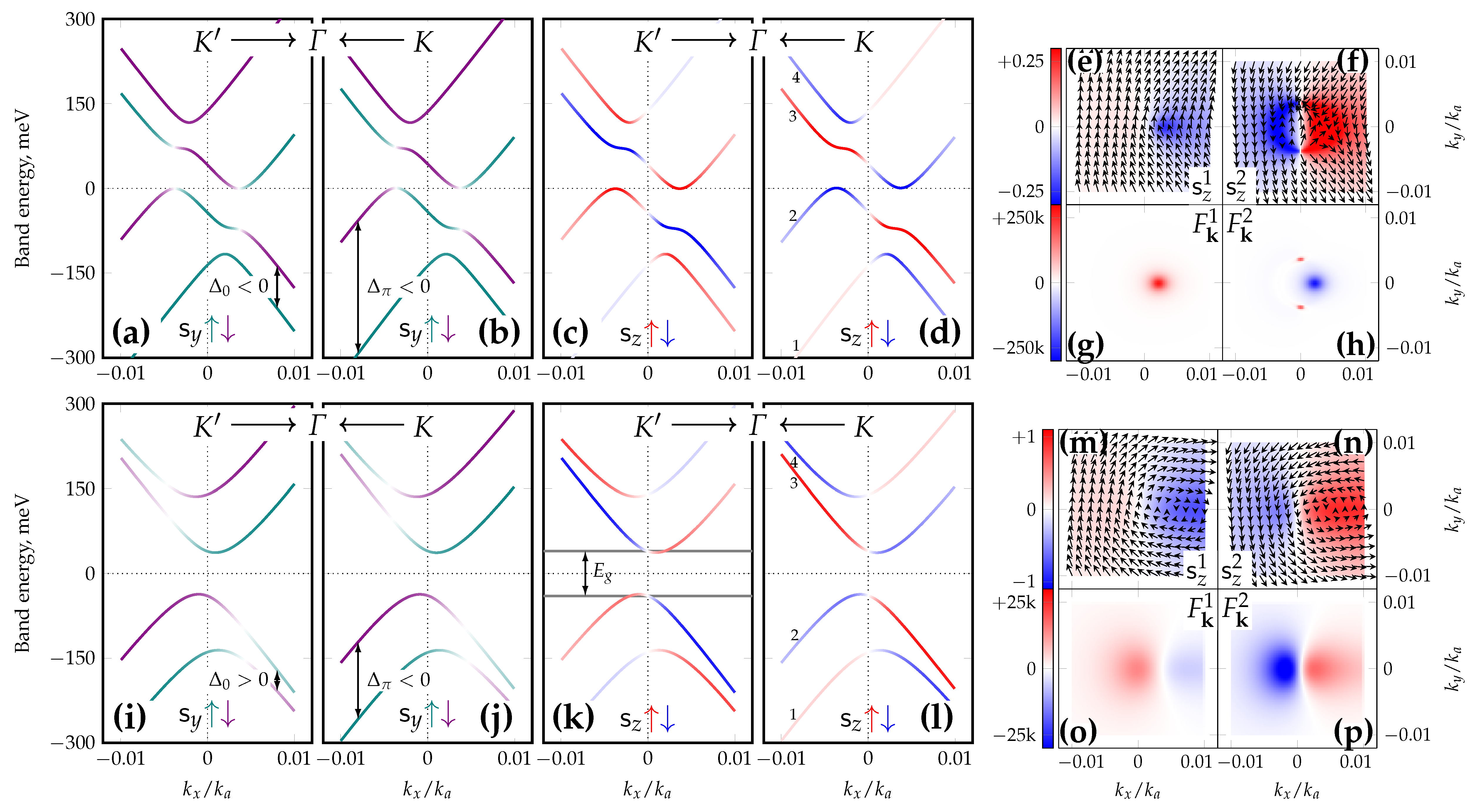
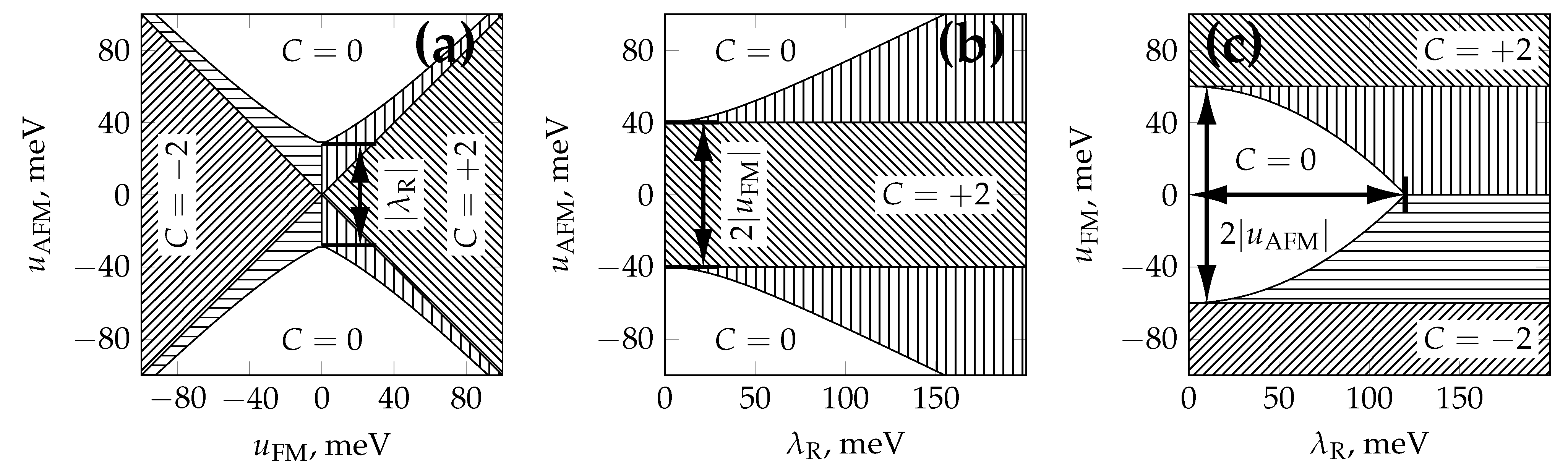
Unlike the previous case of in-plane magnetization, an out-of-plane magnetized system may exhibit a nontrivial band topology. It may be investigated by analyzing band inversions of the Hamiltonian
h ( k ) = u A 0 ε e i ϑ i λ R K 0 u A i λ R K ε e i ϑ ε e i ϑ i λ R K u B 0 i λ R K ε e i ϑ 0 u B
at a particular Dirac point. For example, the Hamiltonian eigenvalues at the K point are u A , u B and u AFM ± u FM 2 + λ R 2 , where the latter pair evolves with changing λ R ; from now on, these levels are called “moving” in contrast to the other pair of “static” eigenvalues. The evolution of all these eigenvalues at the K point under gradual imposition of ferromagnetic and Rashba interactions onto the pure-AFM configuration is depicted in Figure 3 with the corresponding band and spin structures. Implying λ R 0 and defining s = 1 + 4 u A u B λ R 2 , a total of three conceptually distinct possibilities for the band structure may be identified.
  • The | u FM | > | u AFM | condition defines an FM-dominated case where the band structure at both valleys is gapped and inverted ( s z inversion is evident in Figure 3d,e), and the band structure is always characterized by two Dirac rings per valley. The total Chern number is C = 2 sign u FM ; the system is always topologically nontrivial with the valley gap of magnitude
    E g = 2 λ R 2 | u FM | s W RFM 2 centered around E 0 = λ R 2 ν u AFM W RFM 2
    where the gap center E 0 explicitly depends on the valley. The global gap is E g 2 | E 0 | .
  • The inverse condition | u FM | < | u AFM | admits both normal and inverted band structures depending on the λ R value. According to Figure 3f, a small λ R value leads to a normal valley gap (see Figure 3i for the band structure)
    E g = 2 | u AFM | | u FM | u FM 2 + λ R 2 .
  • If the λ R value in the AFM-dominated case is sufficiently large, a band inversion manifests itself at both valleys. The critical value is defined by a zero gap in Equation (9) and is equal to
    10 p t W W W λ R crit = 2 u AFM 2 | u AFM u FM | . 10 p t W W W
When | λ R | is increased past the | λ R crit | value, the gap in Equation (9) reopens as inverted, having the same value up to a sign reversal. However, at another critical λ R value, a Dirac ring emerges at each valley (one within the upper valence band at K and one within the lower conduction band at K or vice versa, depending on the u AFM sign; see Figure 3j). This critical value is
λ R DR = 2 | u AFM | u A u B 2 u A u B
(remember that u A u B < 0 if | u AFM | < | u FM | ). The gap value in this case is
E g = λ R 2 | u FM | s W RFM 2 + | u FM | 1 4 | u FM u AFM | W RFM 2 .
The valley gap magnitudes given above are all defined by the system
ε k ( E k 2 q k ) = 0 , ( extremum condition ) ( E k 2 q k ) 2 W RFM 2 E k 2 2 E k λ R 2 ν u AFM + λ R 2 u A u B = 0 , ( sec ular equation ) q k = ε k 2 u A u B .
Strictly speaking, in the AFM-dominated case with band inversion ( | λ R | > | λ R crit | ), the Chern number will not be an integer since the global gap is closed (indirectly, between K and K valleys), and the Fermi level (here E F = 0 ) crosses the bands at both valleys. The multiparametric topological phase diagrams that are shown in Figure 4 are plotted based only on the band inversion condition in Equation (10). However, if the Fermi level is not accounted for, then the Berry curvature Brillouin zone integral involving only the valence bands is still
1 2 π BZ d k ( F k 1 + F k 2 ) = 2 sign u FM ,
exactly as in the FM-dominated case, which is certainly topological.
Using the earlier definition ε a = ε 2 + u AFM 2 , the μ -Hamiltonian (A7) for the out-of-plane case may be written as
h μ ( k + ν K ) = μ ε a u FM s z + μ λ R 2 1 u AFM ν ε a ( s · [ e z × k ^ ] ) .
The energy splitting Δ ν between the bands directly depends on the valley index ν through the valley term δ :
Δ ν = Δ 0 ν δ , Δ 0 = W RFM = λ R 2 + 4 u FM 2 , δ λ R 2 W RFM u AFM ε a .
The δ term may be perceived as small since it is inversely proportional to the ε a (which may be taken to be 1 2 E k 1 + E k 2 as a good approximation). On the other hand, when the AFM interaction u AFM is sufficiently large, this δ splitting asymmetry may become confidently detected in a spin-resolved experiment due to a large curvature difference between valence bands. For example, Figure 5g,h are supplemented with dash-dotted asymptotic lines that are valley-symmetrically split by Δ 0 on each diagram, but the actual spin-splittings Δ K and Δ K marked by arrows are undoubtedly different, thus highlighting the spin-splitting valley asymmetry.
The spin texture vector for upper valence or conduction bands on the basis of Equation (15) is
n μ ν ( k ) Δ ν 1 μ λ R 1 u AFM ν ε a [ e z × k ^ ] 2 u FM e z .
The in-plane spin texture in the FM-dominated case is similar to a pure Rashba case since spin inversions occur only at the K/ K points (see Figure 5a,b). However, the AFM-dominated case allows for additional spin inversion points, e.g., the AFM-dominated trivial band structure in Figure 5g,h has three spin inversion points for a single band, which eventually deforms to acquire the Dirac ring when | λ R | > | λ R DR | in Equation (11).
Out-of-plane spin textures for the AFM-dominated trivial case are simple (see Figure 5i,j) since the s z spin polarization of all bands is complete and almost uniform. Topological out-of-plane magnetized systems (both FM- and AFM-dominated) are characterized by additional innermost spin inversion regions on their spin texture diagrams for upper valence and lower conduction bands (see Figure 5d; the AFM-dominated topological case is conceptually the same). These regions are exceptional for these bands since the s z spin texture prescribed by Equation (16) is recovered for all bands sufficiently far away from valleys.
Berry curvatures (5) for the FM-dominated case (see Figure 5e,f) have mutually compensating (in the F k 1 + F k 2 sense) sharp peaks for bands #1 and #2 and an additional ring-like structure for band #2, which exactly corresponds to Dirac rings and delivers the nonzero Chern number
C = 1 2 π BZ d k n f n k F n k = 2 sign u FM , f n k = 1 , n = 1 , 2 ( VB ) , 0 , n = 3 , 4 ( CB ) .
The Berry curvature structure for the AFM-dominated topological case is conceptually the same (see also the note on Chern numbers above), and Berry curvatures for the AFM-dominated trivial case has two mutually compensating peaks of different height and width (see Figure 5k,l).
Table 3 summarizes the discussion above for the K Γ K observation direction (along x); the measuring points that correspond to the valley columns are marked in Figure 5a,b,g,h with arrows.

4. Discussion

Based on the detailed model description presented above, one may draw some practical conclusions on the model parameters λ R , u FM , | u AFM | using the results of spin-ARPES observations.

4.1. In-Plane Magnetized Graphene with Rashba Interaction

This case was described in detail in Section 3.1 and is qualitatively simple to assess since the in-plane ferromagnetic component u FM interacts with the Rashba coupling λ R such that these quantities may be decoupled from each other using the splitting asymmetry.
A typical situation is presented in [26] where the magnetization direction m ^ = e y is perpendicular to the K Γ K scanning direction. An instructive example of the ARPES data analysis is the following: the “left” splitting Δ L measured between K and Γ ( ϕ = 0 direction; see Figure 6a) was estimated as Δ L = 40 meV (minus is due to negative s y polarization of the upper valence band at the measuring point), the “right” splitting Δ R measured between Γ and K ( ϕ = π direction; see Figure 6a) was estimated as Δ R = + 80 meV (the upper valence band was positively s y -polarized) and the gap estimate was E g = 80 meV. According to the classification of band and spin textures in Table 1, they are eligible to be classified as gapped and invertible. Since the in-plane spin structure is invertible, then the Rashba interaction dominates (i. e. | λ R | > 2 | u FM | ); however, the Rashba coupling constant is negative because Δ L < 0 (see Table 2). These qualitative reasonings allow quantitative estimates of the model parameters with correct signs:
Δ L = | λ R 2 u FM | = + λ R 2 u FM = 40 meV , Δ R = + | λ R + 2 u FM | = λ R 2 u FM = + 80 meV , E g = λ R 2 + 4 u AFM 2 λ R 2 + 4 u FM 2 = + 80 meV .
The system is easily solved to obtain u FM = 10 meV, λ R = 60 meV, | u AFM | 65 meV (these values slightly differ from [26] where a more accurate computer fitting procedure was used). The problem of the u AFM sign stems from the fact that the u AFM value enters the secular Equation (7) only as a square; hence, the sign cannot be determined from any quantity that is represented by an energy difference (band splitting, gap, etc.). The spin texture cannot decide the sign either; in fact, this sign is reflected only in pseudospin textures.
In the case of any other magnetization direction that makes an angle α with the K Γ K direction, the principle of measuring point selection stays the same: one is advised to find two points (one per each valley) such that ϕ α = ± π 2 in order to acquire the maximum splitting asymmetry, thus reducing the error of u FM and λ R estimation. For example, if the magnetization in the analysis above is m ^ = e x ( α = π ), then the exact same results should be obtained if the measuring points are selected according to Figure 6b (narrow or broad marks on Figure 6 schematically show small and large spin-splittings, respectively).
The example above may be supplemented by the following note. Suppose that no s y spin inversion occurs so that the “left” and “right” splittings have the same sign (per Table 1, the spin texture is thus persistent). In this case, Table 2 may be used to find that the u FM sign corresponds to s y polarization of the lower valence band.
The final remark concerns the zero-gap case where only the fact that | u FM | > | u AFM | may be confidently established; the authors cannot give any practical recommendations based on the studied model to find the u AFM value in this situation.

4.2. Out-of-Plane Magnetized Graphene with Rashba Interaction

This case was described in detail in Section 3.2. It is more interesting than the in-plane case since it admits a nontrivial band topology, so deducing the model parameters from the spin-resolved ARPES data may allow one to suppose whether a given system is a viable candidate for being topologically nontrivial or even to perform material engineering on a system with the purpose of obtaining such a candidate.
The out-of-plane magnetization case is characterized by an explicit spin-splitting valley dependence, which also depends explicitly on the binding energy of a corresponding measuring point as O ( ε 1 ) (see Figure 5g,h). The latter circumstance makes the measuring procedure less stable because the spin-splitting asymmetry is no more an asymptotic quantity (independent from exact position of a measuring point) but quickly diminishes with the ε increase. Interplay between FM and Rashba interactions does not allow isolating u FM and λ R apart since these quantities always enter all relations together as an W RFM quantity. The complexity of E g expressions for analysis present additional difficulties in the estimation of the model parameters. Nevertheless, some recommendations may still be suggested.
First of all, one may choose any convenient ARPES scanning direction; here, the K Γ K direction is chosen. The valley-dependent spin-splittings have the form Δ = W RFM ± δ (see Table 3); one may choose two convenient measurement points k L (on the K Γ segment) and k R (on the Γ K segment) in each valley with approximately equal binding energies E B ( k ) = 1 2 ( E k 1 + E k 2 ) (mean value of two valence band energies) and perform the spin-splitting measurements Δ L and Δ R at these points. The condition of equal binding energies is important because it allows interpreting the measurement results (see Table 3 for spin-splitting sign selection rules)
sign λ R 2 Δ L Δ R = W RFM = λ R 2 + 4 u FM 2 , sign λ R 2 Δ L + Δ R = δ = λ R 2 W RFM u AFM E B 2 + u AFM 2 .
The third equation may be obtained if one measures the energies of valence band maxima E VBM ν in each valley. In certain cases, one may observe ARPES spectra at the valleys that are similar to Figure 5g,h where the difference between E VBM K and E VBM K is significant. In three out of four cases (see Table 3), this difference provides useful information being equal to 2 λ R 2 u AFM W RFM 2 (FM-dominated case) or u FM 2 + λ R 2 | u FM | (AFM-dominated cases without Dirac rings). Another useful observation is that in the AFM-dominated case one of the valence band maxima is always at ± ( u AFM | u FM | ) .
Technically, the provided information above is sufficient to close the system of equations defining the model parameters. Nevertheless, one may attempt to demagnetize a given graphene system completely and check that the band structure reduces to the one displayed in Figure 1c,d, thus verifying the magnetism as the sole source of band structure modification (besides the Rashba coupling), checking the model applicability and finding the “undressed” λ R value directly.

4.3. Multiparametric Topological Phase Diagrams

A trivial fact that is known from the literature is that τ 0 s z exchange-coupled graphene with the Rashba interaction hosts a nontrivial band topology with the total Chern number of ± 2 . In the scope of this paper, such an exchange term is portrayed as a term of a ferromagnetic origin. The topological phase diagrams in Figure 4 contain new information regarding the stability of this nontrivial topology with respect to antiferromagnetic interactions.
As was noted before, the valley topology is nontrivial if either | u FM | > | u AFM | with any λ R 0 or if | u FM | < | u AFM | while | λ R | > | λ R crit | . In the latter case, the global gap is closed, but each valley gap is opened and inverted; hence, the total Chern number is not identically zero but is not an integer either.
Figure 4a depicts the u FM - u AFM topological phase diagram for a fixed λ R = + 56 meV. The plane is divided into five regions: a trivial disconnected region C = 0 with no hatching, two “perfect” FM-dominated nontrivial regions C = 2 sign u FM with slanted hatchings and two “imperfect” nontrivial regions with closed global gap, which are hatched accordingly (hatch lines are horizontal for C < 0 and vertical otherwise). This figure essentially shows that the AFM interaction is detrimental to the topological properties of the magneto-spin–orbit graphene and also points to the fact that the topological phase destruction is, in fact, smooth under the u AFM increase: it does not occur abruptly but instead the Hall conductance undergoes gradual degradation. The extent of nontrivial band topology persistence under AFM interaction may also be evaluated as the size of the “imperfect” regions, which is on the order of λ R .
Figure 4b gives clearer insight into how the Rashba interaction helps overcome the detrimental AFM interaction. Although the main “perfect” region with C = + 2 is the strip of 2 | u FM | width, the system may possess nonzero Hall conductance even when its phase point lies outside of the strip but inside the vertically hatched “imperfect” area with the width proportional to | λ R | value.
Figure 4c shows the situation from the ferromagnetic exchange perspective. The system topology is usually nontrivial everywhere except the compact unhatched trivial region; in particular, even the smallest nonzero u FM values may give nonzero (albeit imperfectly quantized) Hall conductance, provided the Rashba strength overcomes the AFM interaction. By comparing this subfigure with others, one may notice that the vertical size of the trivial region is also 2 | u AFM | .

5. Conclusions

This paper deals with the simple tight-binding model of magneto-spin–orbit graphene based on certain premises supported by experimental data found in the literature. This tight-binding model incorporates the Rashba coupling and general collinear sublattice ferrimagnetism for arbitrary magnetizations m A and m B . Two magnetization direction variants are analyzed for arbitrary magnetization energies: the in-plane case m ^ = m x e x + m y e y and the out-of-plane case m ^ = e z .
It is established that in-plane systems are topologically trivial, characterized by spin canting and Berry curvature dipoles, and their band and spin structures allow the model parameters to be found from spin-ARPES observations through a rather easy procedure. If the FM interaction dominates, then the band structure is gapless at each valley and the spin texture is rather complex; the reverse is true for the AFM-dominated case. Only these in-plane magnetized systems were experimentally studied in the context of the magneto-spin–orbit graphene problem to this day; although they are topologically trivial, their Berry curvature dipoles may render them interesting and promising research objects from both theoretical and experimental points of view since the same structures have already been reported for other two-dimentsional systems with strong spin–orbit coupling.
The out-of-plane magnetization allows nontrivial band topology in both FM- and AFM-dominated cases, but the anomalous Hall conductance may perfectly quantize in the FM-dominated regime only since the AFM-dominated nontrivial situation is characterized by a zero global gap. Additionally, the model parameters cannot be found from the experimental data as simply as in the in-plane case due to the fact that the primary method of evaluating the Rashba coupling constant by valence band spin-splitting near the Dirac point yields only its particular combination with FM coupling, not the pure λ R value. This means that more sophisticated procedures are to be employed; however, it is still theoretically possible to deduce the system topology from the experimental spectra. The creation of such out-of-plane magnetized systems remains, of course, an important problem in the context of experimental QAHE in graphene. This article may aid experimenters who try to solve the problem of proper system synthesis by providing an indirect method of testing candidate systems for QAHE possibility by using only the relatively accessible spin-ARPES technique.

Author Contributions

Conceptualization, A.G.R. and A.V.T.; methodology, A.V.E.; software, A.V.E.; validation, A.G.R.; formal analysis, A.V.E.; investigation, A.V.E., A.V.T. and A.G.R.; resources, A.M.S. and A.G.R.; data curation, A.V.E.; writing—original draft preparation, A.V.E.; writing—review and editing, A.V.E., A.V.T., A.G.R. and A.M.S.; visualization, A.V.E.; supervision, A.M.S. and A.G.R.; project administration, A.G.R.; funding acquisition, A.M.S. All authors have read and agreed to the published version of the manuscript.

Funding

This research was funded by the Saint Petersburg State University grant No. 94031444.

Institutional Review Board Statement

Not applicable.

Informed Consent Statement

Not applicable.

Data Availability Statement

Not applicable.

Acknowledgments

The authors acknowledge the Laboratory of electronic and spin structure of nanosystems of St. Petersburg State University for the support and the use of facilities.

Conflicts of Interest

The authors declare no conflict of interest.

Abbreviations

The following abbreviations are used in this manuscript:
ARPESAngle-resolved photoelectron spectroscopy
spin-ARPESSpin- and angle-resolved photoelectron spectroscopy
DFTDensity functional theory
STMScanning tunnel microscopy
QAHEQuantum anomalous Hall effect
FMFerromagnetism, ferromagnetic coupling
AFMAntiferromagnetism, antiferromagnetic coupling
FIMFerrimagnetism, combination of FM and AFM couplings
VBValence band
CBConduction band
DRDirac ring

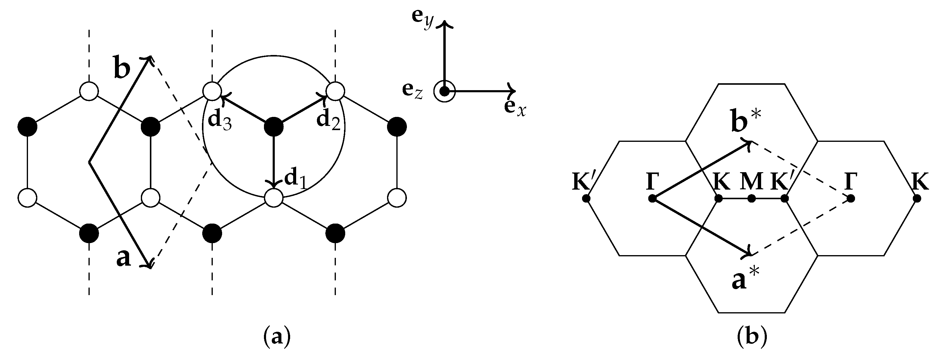
Appendix A. Model Geometry

This section establishes a certain Brillouin zone orientation that is used throughout the text and is shown in Figure A1 with respect to Cartesian axes, where the following identities hold:
a = a ( e x cos 60 e y sin 60 ) , a * = k a ( e x cos 30 e y sin 30 ) , b = a ( e x cos 60 + e y sin 60 ) , b * = k a ( e x cos 30 + e y sin 30 ) , d 1 = d e y = a b 3 , d 2 = d 1 + b , d 3 = d 1 a
which are related as a a * = b b * = a · k a cos 30 = 2 π , k a = 4 π a 3 = 4 π 3 d . The valley index ν = ± 1 is introduced to denote valley centers as ν K since
K = a * + b * 3 = k a 3 e x , K = K = k a 3 e x .
The along- Γ K directions are thus defined by k y = 0 , and ortho- Γ K directions are defined by k x = ν K x . The following expansions are valid near the K valley, ϕ k = arg ( k x + i k y ) :
f ( k + K ) = 3 k d 2 e i ϕ k + o ( k ) , rot f ( k + K ) = 3 d 2 ( i e x + e y ) + o ( 1 ) .
Similar relations for the other valley can be obtained using f ( k ) = f * ( k ) .
Figure A1. Graphene direct and reciprocal lattice with coordinate axes. (a) Fragment of direct space lattice with translation vectors and nearest-neighbour A B hopping vectors d i . Filled circles: sublattice A, empty circles: sublattice B. (b) Fragment of reciprocal lattice. Reciprocal vectors together with dashed lines form a primitive Brillouin zone.
Symmetry 15 00516 g0a1

Appendix B. Graphene with One Kind of Interactions

Appendix B.1. Principal Hopping Integral

In the absence of any interactions, the Hamiltonian and its eigenvalues are
h ( k ) = 0 ε e i ϑ ε e i ϑ 0 , E μ σ = μ ε = μ t | f ( k ) |
where the pseudospin structure of SU(2) spin-degenerate eigenstates is determined by the phase angle ϑ ( k ) . The eigenstates μ σ of the Hamiltonian h ( k ) are the usual tensor products μ σ , where μ = + 1 denote valence band states and μ = 1 denote conduction band states, σ = ± 1 being the usual spinors for spins ↑ or ↓, respectively. According to Equation (A1), the band structure slope k E ( k ) is 3 2 d t , and it can be read off the ARPES data directly (see Figure 1a). The positive hopping integral t is then derived from
t [ eV ] 0.4695 × k E ( k ) eV Å 1 .

Appendix B.2. Standard Rashba Splitting

If only the Rashba interaction is present, the Hamiltonian is
h ( k + ν K ) = 0 ε e i ϑ + R ε e i ϑ + R 0 , R = λ R 3 d ( s · rot f ) 0 i λ R K i λ R K 0 , λ R K = λ R 1 + ν 2 , λ R K = λ R 1 ν 2 .
The band dispersion in the K Γ K direction with the corresponding in-plane s y spin texture is depicted in Figure 1c,d where the dispersion law is
E μ ( k ) = ± λ R 2 μ λ R 2 4 + ε 2
and the in-plane spin-momentum locked spin texture is defined by the μ -Hamiltonian (A7)
h μ ( k + ν K ) = μ ε + μ λ R 2 ( s · [ e z × k ^ ] ) .
When the K Γ K path is scanned, the splittings between valence bands may be conveniently measured at points between Γ and one of the Dirac points, as is marked with arrows in Figure 1c,d. Due to the spin-momentum locking, the electronic states are completely spin-polarized perperndicularly to the ARPES scanning direction. This paper uses the geometry in Figure A1 where the K Γ K path lies in the x-direction, thus implying a complete y-spin polarization. The relevant discussion is summarized in Table A1.
Table A1. Spin polarizations and splittings for pure Rashba interaction, the along- Γ K x-direction.
Valley K K
Upper VB, s y spin + sign λ R sign λ R
Lower VB, s y spin sign λ R + sign λ R
Signed splitting + λ R λ R

Appendix B.3. Valley Gap
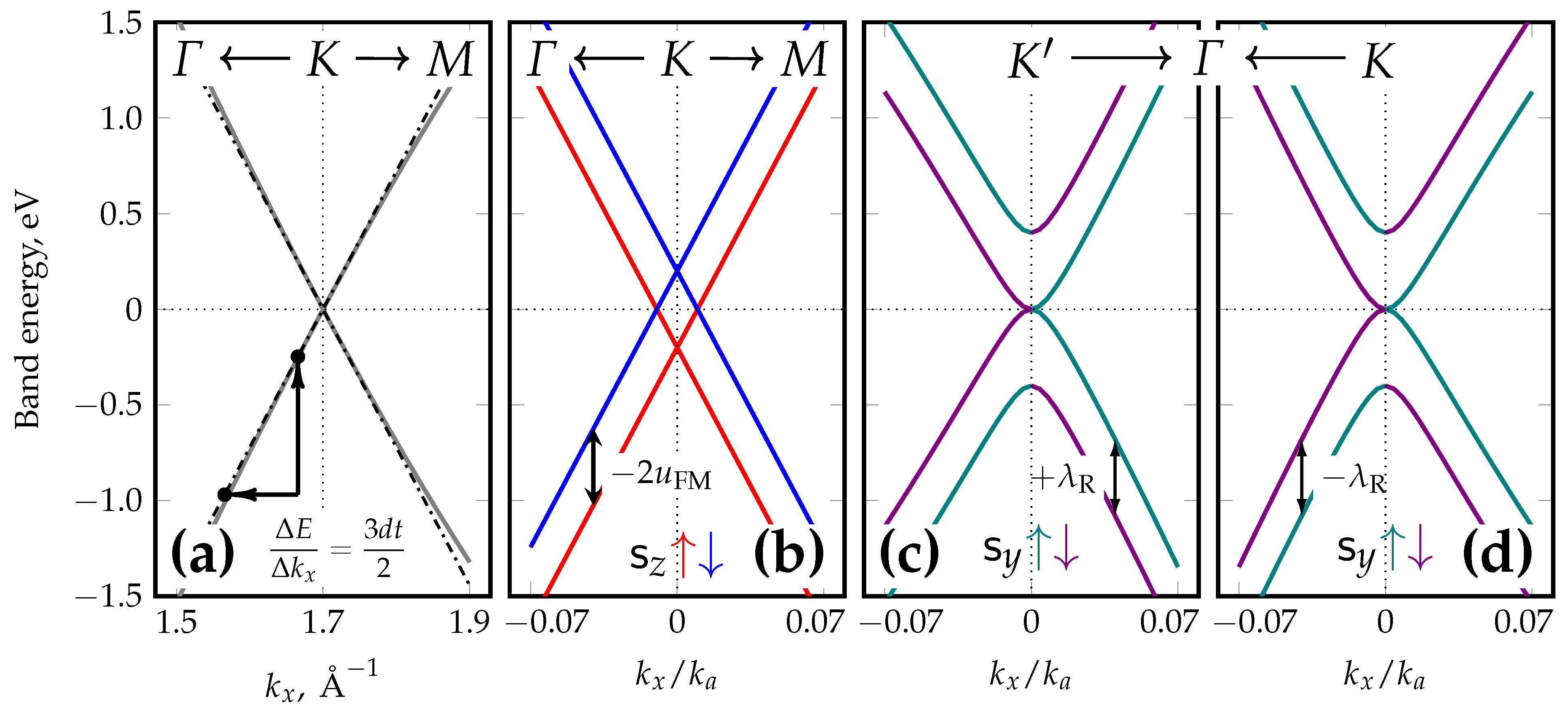
If graphene is magnetized only, then the SU(2) spin symmetry allows interpreting the z-direction to contain the magnetization vector m ^ ; the Hamiltonian is
h ( k ) = u A s z ε e i ϑ s 0 ε e i ϑ s 0 u B s z = u FM s z 0 0 u FM s z u AFM s z ε e i ϑ s 0 ε e i ϑ s 0 u AFM s z .
The following three cases with respect to u FM and u AFM values may be identified.
  • If u AFM = 0 , the resulting band dispersion consists of two completely spin-polarized standard graphene dispersions split by 2 u FM (see Figure 1b). The eigenvectors μ σ match those for pristine graphene, but the energy eigenvalues are
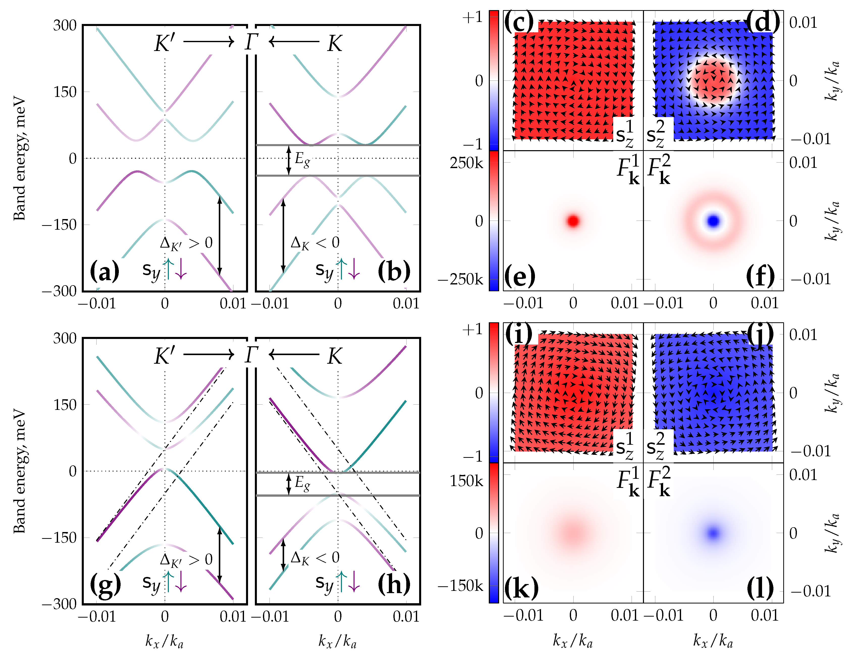
    E μ σ FM ( k ) = μ ε σ u FM .
  • If u FM = 0 , the spin-degenerate bands with a gap of magnitude 2 | u AFM | are given by (see Figure 3b)
    E μ σ AFM ( k ) = μ ε AFM μ u AFM 2 + ε 2 .
    These bands have a meron-like [51] pseudospin texture where the pseudospin vector is directed along ε ε a e x cos ϑ k + ε ε a e y sin ϑ k + σ u AFM ε a e z . In particular, it is directed along e z at the Dirac points (where ε = 0 ), which signals a complete sublattice localization of the corresponding electronic states.
  • If both u FM and u AFM are nonzero, then a ferrimagnetic configuration is established giving the band dispersions
    E μ σ FIM ( k ) = μ ε AFM σ u FM .
    with the spin-splitting of 2 u FM . When the sublattice magnetizations are -aligned, FM interaction dominates, and the corresponding band structure has an FM-like character (see Figure 3c). Conversely, another FIM case presents when the moments are -aligned; AFM interaction then dominates (see Figure 3h) and a finite gap of
    E g = 2 max 0 , | u AFM | | u FM |
    opens up. The presence of a sufficiently large band gap on ARPES spectra is a clear sign that a significant AFM interaction is involved if no other sources of sublattice symmetry breaking are evident.

Appendix C. Valence and Conduction Band Hamiltonians

The spin Hamiltonians used in the paper to obtain splittings and spin textures between valence bands and between conduction bands are derived using the intermediate diagonalization procedure. Suppose that the Hamiltonian in the { A , A , B , B } basis is written as h τ σ and is transformed into another basis { A , B , A , B } (here, z ¯ is the complex conjugate of z):
h τ σ = h A A h A A h A B h A B h ¯ A A h A A h A B h A B h ¯ A B h ¯ A B h B B h B B h ¯ A B h ¯ A B h ¯ B B h B B σ τ h A A h A B h A A h A B h ¯ A B h B B h ¯ A B h B B h ¯ A A h A B h A A h A B h ¯ A B h ¯ B B h ¯ A B h B B = h h h h h σ τ
The main diagonal 2 × 2 spin blocks h and h are diagonalized as
Ω σ h σ σ Ω σ = diag ( E σ μ = + 1 , E σ μ = 1 )
where E σ μ = + 1 E σ μ = 1 . The whole 4 × 4 Hamiltonian is then transformed as follows:
h σ τ Ω Ω 0 0 Ω h h h h Ω 0 0 Ω = E μ = + 1 0 w 11 w 12 0 E μ = 1 w 21 w 22 w ¯ 11 w ¯ 21 E μ = + 1 0 w ¯ 12 w ¯ 22 0 E μ = 1
where W = Ω h Ω . The last step is to exchange second and third elements in the basis, which results in the μ σ Hamiltonian:
h μ σ = E μ = + 1 w 11 0 w 12 w ¯ 11 E μ = + 1 w ¯ 21 0 0 w 21 E μ = 1 w 22 w ¯ 12 0 w ¯ 22 E μ = 1 = h μ = + 1 W 1 W 1 h μ = 1 ,
here, h μ is the 2 × 2 Hamiltonian that the reader might have encountered throughout this paper. Elements of W 1 share the same order of magnitude as the interaction energies u FM , u AFM , λ R , whereas the eigenvalues of h μ are roughly proportional to the kinetic energy ε = t | f ( k ) | ; hence, the matrix W 1 that defines the interaction between valence and conduction bands may be neglected entirely in the zeroth-order perturbation theory framework.

References

  1. Chowdhury, T.; Sadler, E.C.; Kempa, T.J. Progress and Prospects in Transition-Metal Dichalcogenide Research Beyond 2D. Chem. Rev. 2020, 120, 12563–12591. [Google Scholar] [CrossRef] [PubMed]
  2. Yin, X.; Tang, C.S.; Zheng, Y.; Gao, J.; Wu, J.; Zhang, H.; Chhowalla, M.; Chen, W.; Wee, A.T.S. Recent developments in 2D transition metal dichalcogenides: Phase transition and applications of the (quasi-)metallic phases. Chem. Soc. Rev. 2021, 50, 10087–10115. [Google Scholar] [CrossRef]
  3. Habib, M.R.; Wang, W.; Khan, A.; Khan, Y.; Obaidulla, S.M.; Pi, X.; Xu, M. Theoretical Study of Interfacial and Electronic Properties of Transition Metal Dichalcogenides and Organic Molecules Based van der Waals Heterostructures. Adv. Theory Simulat. 2020, 3, 2000045. [Google Scholar] [CrossRef]
  4. Mu, H.; Yu, W.; Yuan, J.; Lin, S.; Zhang, G. Interface and surface engineering of black phosphorus: A review for optoelectronic and photonic applications. Mater. Futur. 2022, 1, 012301. [Google Scholar] [CrossRef]
  5. Burch, K.S.; Mandrus, D.; Park, J.G. Magnetism in two-dimensional van der Waals materials. Nature 2018, 563, 47–52. [Google Scholar] [CrossRef] [PubMed]
  6. Wang, D.; Tang, F.; Ji, J.; Zhang, W.; Vishwanath, A.; Po, H.C.; Wan, X. Two-dimensional topological materials discovery by symmetry-indicator method. Phys. Rev. B 2019, 100, 195108. [Google Scholar] [CrossRef] [Green Version]
  7. Weiss, N.O.; Zhou, H.; Liao, L.; Liu, Y.; Jiang, S.; Huang, Y.; Duan, X. Graphene: An Emerging Electronic Material. Adv. Mater. 2012, 24, 5782–5825. [Google Scholar] [CrossRef]
  8. Falkovsky, L.A. Optical properties of graphene. J. Phys. Conf. Ser. 2008, 129, 012004. [Google Scholar] [CrossRef] [Green Version]
  9. Wimmer, M.; Adagideli, I.D.I.M.C.; Berber, S.M.C.; Tománek, D.; Richter, K. Spin Currents in Rough Graphene Nanoribbons: Universal Fluctuations and Spin Injection. Phys. Rev. Lett. 2008, 100, 177207. [Google Scholar] [CrossRef] [Green Version]
  10. Chen, S.H.; Nikolić, B.K.; Chang, C.R. Inverse quantum spin Hall effect generated by spin pumping from precessing magnetization into a graphene-based two-dimensional topological insulator. Phys. Rev. B 2010, 81, 035428. [Google Scholar] [CrossRef]
  11. Han, W.; McCreary, K.; Pi, K.; Wang, W.; Li, Y.; Wen, H.; Chen, J.; Kawakami, R. Spin transport and relaxation in graphene. J. Magn. Magn. Mater. 2012, 324, 369–381. [Google Scholar] [CrossRef] [Green Version]
  12. Rybkina, A.A.; Rybkin, A.G.; Adamchuk, V.K.; Marchenko, D.; Varykhalov, A.; Barriga, J.S.; Shikin, A.M. The graphene/Au/Ni interface and its application in the construction of a graphene spin filter. Nanotechnology 2013, 24, 295201. [Google Scholar] [CrossRef] [PubMed]
  13. Rybkina, A.A.; Rybkin, A.G.; Klimovskikh, I.I.; Skirdkov, P.N.; Zvezdin, K.A.; Zvezdin, A.K.; Shikin, A.M. Advanced graphene recording device for spin–orbit torque magnetoresistive random access memory. Nanotechnology 2020, 31, 165201. [Google Scholar] [CrossRef] [PubMed]
  14. Kamalakar, M.V.; Groenveld, C.; Dankert, A.; Dash, S. Long distance spin communication in chemical vapour deposited graphene. Nat. Commun. 2015, 6, 6766. [Google Scholar] [CrossRef] [PubMed] [Green Version]
  15. Zatko, V.; Dubois, S.M.M.; Godel, F.; Galbiati, M.; Peiro, J.; Sander, A.; Carretero, C.; Vecchiola, A.; Collin, S.; Bouzehouane, K.; et al. Almost Perfect Spin Filtering in Graphene-Based Magnetic Tunnel Junctions. ACS Nano 2022, 16, 14007–14016. [Google Scholar] [CrossRef] [PubMed]
  16. Konschuh, S.; Gmitra, M.; Fabian, J. Tight-binding theory of the spin-orbit coupling in graphene. Phys. Rev. B 2010, 82, 245412. [Google Scholar] [CrossRef] [Green Version]
  17. Rashba, E.I. Graphene with structure-induced spin-orbit coupling: Spin-polarized states, spin zero modes, and quantum Hall effect. Phys. Rev. B 2009, 79, 161409. [Google Scholar] [CrossRef] [Green Version]
  18. Shikin, A.M.; Rybkina, A.A.; Rybkin, A.G.; Klimovskikh, I.I.; Skirdkov, P.N.; Zvezdin, K.A.; Zvezdin, A.K. Spin current formation at the graphene/Pt interface for magnetization manipulation in magnetic nanodots. Appl. Phys. Lett. 2014, 105, 042407. [Google Scholar] [CrossRef]
  19. Shikin, A.M.; Rybkin, A.G.; Marchenko, D.; Rybkina, A.A.; Scholz, M.R.; Rader, O.; Varykhalov, A. Induced spin–orbit splitting in graphene: The role of atomic number of the intercalated metal and πd hybridization. New J. Phys. 2013, 15, 013016. [Google Scholar] [CrossRef] [Green Version]
  20. Klimovskikh, I.I.; Otrokov, M.M.; Voroshnin, V.Y.; Sostina, D.; Petaccia, L.; Di Santo, G.; Thakur, S.; Chulkov, E.V.; Shikin, A.M. Spin–Orbit Coupling Induced Gap in Graphene on Pt(111) with Intercalated Pb Monolayer. ACS Nano 2017, 11, 368–374. [Google Scholar] [CrossRef]
  21. Marchenko, D.; Varykhalov, A.; Sánchez-Barriga, J.; Seyller, T.; Rader, O. Rashba splitting of 100 meV in Au-intercalated graphene on SiC. Appl. Phys. Lett. 2016, 108, 172405. [Google Scholar] [CrossRef] [Green Version]
  22. Otrokov, M.M.; Klimovskikh, I.I.; Calleja, F.; Shikin, A.M.; Vilkov, O.; Rybkin, A.G.; Estyunin, D.; Muff, S.; Dil, J.H.; de Parga, A.L.V.; et al. Evidence of large spin-orbit coupling effects in quasi-free-standing graphene on Pb/Ir(111). 2D Mater. 2018, 5, 035029. [Google Scholar] [CrossRef]
  23. Zhizhin, E.; Varykhalov, A.; Rybkin, A.; Rybkina, A.; Pudikov, D.; Marchenko, D.; Sánchez-Barriga, J.; Klimovskikh, I.; Vladimirov, G.; Rader, O.; et al. Spin splitting of Dirac fermions in graphene on Ni intercalated with alloy of Bi and Au. Carbon 2015, 93, 984–996. [Google Scholar] [CrossRef]
  24. Marchenko, D.; Varykhalov, A.; Scholz, M.R.; Bihlmayer, G.; Rashba, E.I.; Rybkin, A.; Shikin, A.M.; Rader, O. Giant Rashba splitting in graphene due to hybridization with gold. Nat. Commun. 2012, 3, 1232. [Google Scholar] [CrossRef] [PubMed] [Green Version]
  25. Rybkin, A.G.; Rybkina, A.A.; Otrokov, M.M.; Vilkov, O.Y.; Klimovskikh, I.I.; Petukhov, A.E.; Filianina, M.V.; Voroshnin, V.Y.; Rusinov, I.P.; Ernst, A.; et al. Magneto-Spin–Orbit Graphene: Interplay between Exchange and Spin–Orbit Couplings. Nano Lett. 2018, 18, 1564–1574. [Google Scholar] [CrossRef] [PubMed]
  26. Rybkin, A.G.; Tarasov, A.V.; Rybkina, A.A.; Usachov, D.Y.; Petukhov, A.E.; Eryzhenkov, A.V.; Pudikov, D.A.; Gogina, A.A.; Klimovskikh, I.I.; Di Santo, G.; et al. Sublattice Ferrimagnetism in Quasifreestanding Graphene. Phys. Rev. Lett. 2022, 129, 226401. [Google Scholar] [CrossRef]
  27. Weser, M.; Rehder, Y.; Horn, K.; Sicot, M.; Fonin, M.; Preobrajenski, A.B.; Voloshina, E.N.; Goering, E.; Dedkov, Y.S. Induced magnetism of carbon atoms at the graphene/Ni(111) interface. Appl. Phys. Lett. 2010, 96, 012504. [Google Scholar] [CrossRef] [Green Version]
  28. Voroshnin, V.; Tarasov, A.; Bokai, K.; Chikina, A.; Senkovskiy, B.; Ehlen, N.; Usachov, D.; Grüneis, A.; Krivenkov, M.; Sánchez-Barriga, J.; et al. Direct Spectroscopic Evidence of Magnetic Proximity Effect in MoS2 Monolayer on Graphene/Co. ACS Nano 2022, 16, 7448–7456. [Google Scholar] [CrossRef]
  29. Piquemal-Banci, M.; Galceran, R.; Dubois, S.M.M.; Zatko, V.; Galbiati, M.; Godel, F.; Martin, M.B.; Weatherup, R.S.; Petroff, F.; Fert, A.; et al. Spin filtering by proximity effects at hybridized interfaces in spin-valves with 2D graphene barriers. Nat. Commun. 2020, 11, 5670. [Google Scholar] [CrossRef] [PubMed]
  30. Tang, C.; Zhang, Z.; Lai, S.; Tan, Q.; Gao, W.b. Magnetic Proximity Effect in Graphene/CrBr3 van der Waals Heterostructures. Adv. Mater. 2020, 32, 1908498. [Google Scholar] [CrossRef] [PubMed]
  31. Karpiak, B.; Cummings, A.W.; Zollner, K.; Vila, M.; Khokhriakov, D.; Hoque, A.M.; Dankert, A.; Svedlindh, P.; Fabian, J.; Roche, S.; et al. Magnetic proximity in a van der Waals heterostructure of magnetic insulator and graphene. 2D Mater. 2019, 7, 015026. [Google Scholar] [CrossRef]
  32. Kaverzin, A.A.; Ghiasi, T.S.; Dismukes, A.H.; Roy, X.; van Wees, B.J. Spin injection by spin–charge coupling in proximity induced magnetic graphene. 2D Mater. 2022, 9, 045003. [Google Scholar] [CrossRef]
  33. Varykhalov, A.; Sánchez-Barriga, J.; Shikin, A.M.; Biswas, C.; Vescovo, E.; Rybkin, A.; Marchenko, D.; Rader, O. Electronic and Magnetic Properties of Quasifreestanding Graphene on Ni. Phys. Rev. Lett. 2008, 101, 157601. [Google Scholar] [CrossRef]
  34. Jacobsen, J.; Pleth Nielsen, L.; Besenbacher, F.; Stensgaard, I.; Lægsgaard, E.; Rasmussen, T.; Jacobsen, K.W.; Nørskov, J.K. Atomic-Scale Determination of Misfit Dislocation Loops at Metal-Metal Interfaces. Phys. Rev. Lett. 1995, 75, 489–492. [Google Scholar] [CrossRef] [Green Version]
  35. Haldane, F.D.M. Model for a Quantum Hall Effect without Landau Levels: Condensed-Matter Realization of the “Parity Anomaly”. Phys. Rev. Lett. 1988, 61, 2015–2018. [Google Scholar] [CrossRef] [Green Version]
  36. Kane, C.L.; Mele, E.J. Quantum Spin Hall Effect in Graphene. Phys. Rev. Lett. 2005, 95, 226801. [Google Scholar] [CrossRef] [PubMed] [Green Version]
  37. Voloshina, E.; Dedkov, Y. Realistic Large-Scale Modeling of Rashba and Induced Spin–Orbit Effects in Graphene/High-Z-Metal Systems. Adv. Theory Simulat. 2018, 1, 1800063. [Google Scholar] [CrossRef]
  38. Sławińska, J.; Cerdá, J.I. Complex spin texture of Dirac cones induced via spin-orbit proximity effect in graphene on metals. Phys. Rev. B 2018, 98, 075436. [Google Scholar] [CrossRef] [Green Version]
  39. Sławińska, J.; Cerdá, J.I. Spin–orbit proximity effect in graphene on metallic substrates: Decoration versus intercalation with metal adatoms. New J. Phys. 2019, 21, 073018. [Google Scholar] [CrossRef]
  40. Takenaka, H.; Sandhoefner, S.; Kovalev, A.A.; Tsymbal, E.Y. Magnetoelectric control of topological phases in graphene. Phys. Rev. B 2019, 100, 125156. [Google Scholar] [CrossRef]
  41. López, A.; Colmenárez, L.; Peralta, M.; Mireles, F.; Medina, E. Proximity-induced spin-orbit effects in graphene on Au. Phys. Rev. B 2019, 99, 085411. [Google Scholar] [CrossRef] [Green Version]
  42. Peralta, M.; Medina, E.; Mireles, F. Proximity-induced exchange and spin-orbit effects in graphene on Ni and Co. Phys. Rev. B 2019, 99, 195452. [Google Scholar] [CrossRef] [Green Version]
  43. Zhou, J.; Sun, Q.; Jena, P. Valley-Polarized Quantum Anomalous Hall Effect in Ferrimagnetic Honeycomb Lattices. Phys. Rev. Lett. 2017, 119, 046403. [Google Scholar] [CrossRef] [PubMed] [Green Version]
  44. Offidani, M.; Ferreira, A. Anomalous Hall Effect in 2D Dirac Materials. Phys. Rev. Lett. 2018, 121, 126802. [Google Scholar] [CrossRef] [Green Version]
  45. Zou, J.; Yuan, Y.; Kang, J. Spin and spin-valley Hall effects in a honeycomb lattice with antiferromagnetism and spin-orbit couplings. Phys. Lett. A 2019, 383, 3162–3166. [Google Scholar] [CrossRef]
  46. Zhou, Y.; Liu, F. Realization of an Antiferromagnetic Superatomic Graphene: Dirac Mott Insulator and Circular Dichroism Hall Effect. Nano Lett. 2021, 21, 230–235. [Google Scholar] [CrossRef] [PubMed]
  47. Han, Y.; Yan, Z.; Li, Z.; Xu, X.; Zhang, Z.; Niu, Q.; Qiao, Z. Large Rashba Spin-Orbit Coupling and High-Temperature Quantum Anomalous Hall Effect in Re-Intercalated Graphene/CrI3 Heterostructure. arXiv 2022, arXiv:2203.16429. [Google Scholar]
  48. Qiao, Z.; Ren, W.; Chen, H.; Bellaiche, L.; Zhang, Z.; MacDonald, A.H.; Niu, Q. Quantum Anomalous Hall Effect in Graphene Proximity Coupled to an Antiferromagnetic Insulator. Phys. Rev. Lett. 2014, 112, 116404. [Google Scholar] [CrossRef] [Green Version]
  49. Phong, V.T.; Walet, N.R.; Guinea, F. Effective interactions in a graphene layer induced by the proximity to a ferromagnet. 2D Mater. 2017, 5, 014004. [Google Scholar] [CrossRef] [Green Version]
  50. Qiao, Z.; Jiang, H.; Li, X.; Yao, Y.; Niu, Q. Microscopic theory of quantum anomalous Hall effect in graphene. Phys. Rev. B 2012, 85, 115439. [Google Scholar] [CrossRef] [Green Version]
  51. Guo, C.; Xiao, M.; Guo, Y.; Yuan, L.; Fan, S. Meron Spin Textures in Momentum Space. Phys. Rev. Lett. 2020, 124, 106103. [Google Scholar] [CrossRef] [PubMed]
Figure 1. Graphene dispersion maps involving none or only one kind of interactions. The bottom axis tick positions on all subfigures match identically, but the values are expressed in different units (absolute and relative): (a) Bands of pristine graphene in the along- Γ K direction (solid gray lines) with their linear parts (dash-dotted black lines); (b) Completely spin-polarized bands of out-of-plane ferromagnetic graphene. The sign of u FM (here positive) determines the spin ordering which is reflected in the sign of the denoted splitting E VB E VB (here negative). (c,d) Spin-momentum locked bands of graphene under pure Rashba spin–orbit coupling where the splitting sign depends on the valley. Here, λ R > 0 ensures positive splitting at the K valley in the K Γ direction, and its value of 400 meV is exaggerated with respect to usual observations (up to 200 meV) for better visibility.
Symmetry 15 00516 g001
Figure 2. Band structures, spin textures and Berry curvatures for the in-plane FIM case, magnetization direction m ^ = e y . First row, figures (ah): gapless FM-dominated case ( u FM = 80 meV, u AFM = 25 meV, λ R = 80 meV) with the following layout: (a,b) contain spin-splitting marks and s y spin textures (full color range, 1 1 ), (cf) contain s z spin textures with the same color key, (g,h) present Berry curvatures of bands #1 and #2 (lower and upper valence bands, respectively). The right panel images (eh) depict only the K valley. The s z color maps are supplemented with in-plane spin texture for the same band. Second row, figures (ip): gapped AFM-dominated case ( u FM = 30 meV, u AFM = 80 meV, λ R = 80 meV) with same layout as for the first row. Absence (presence) of s y spin-splitting inversion is determined by 2 | u FM | > | λ R | (or vice versa) condition. The corresponding inversion points are shifted perpendicular to the magnetization direction from the Dirac points (this affects F k 1 as well). However, s z spin-splitting inversion occurs exactly at the Dirac points which F k 2 also reflects. Two sharp peaks (red) on F k 2 diagram in Figure (h) are characteristic of valence (#2) and conduction (#3) touching bands.
Symmetry 15 00516 g002
Figure 3. Energy splitting scheme at the K valley for out-of-plane mixed Rashba–exchange interactions. First row, figures (ae): the FM-dominated case ( u FM = 80 meV, u AFM = 25 meV, λ R = 80 meV) with energy level diagram and corresponding band structures, s z spin coloring in full range ( 1 1 ). Gray lines on the band diagrams represent the levels from the energy level diagram: solid lines for “moving” levels and dash-dotted lines for “static” levels. Second row, figures (fj): AFM-dominated case ( u FM = 30 meV, u AFM = 80 meV, λ R = 80 meV) with the same layout. Topological phases are marked with their Chern numbers ( E F position is not accounted for). Left vertical axis labels correspond to energy values u i with u dropped for better visibility.
Symmetry 15 00516 g003
Figure 4. Topological phase diagrams resulting from Equation (10). Each figure contains regions with different hatching: slanted hatching for topologically nontrivial regions with perfectly quantized Chern numbers; vertical ( C > 0 ) or horizontal ( C < 0 ) hatchings for topologically nontrivial regions with nonzero but not integer Chern numbers due to the global gap absence; and no hatching is employed for topologically trivial regions. The characteristic dimensions of important regions are marked with arrows. Each subfigure has one of the following parameters fixed, leaving two others as independent variables: λ R = + 56 meV in (a), u FM = + 40 meV in (b) and u AFM = + 60 meV in (c).
Symmetry 15 00516 g004
Figure 5. Band structures, spin textures and Berry curvatures for the out-of-plane FIM case. First row, Figures (af): the FM-dominated case from Figure 3d with the following layout: (a,b) contain spin-splitting marks, s y spin textures (full color range, 1 1 ) and dash-dotted band asymptotes as references, (c,d) contain s z spin textures and (e,f) present Berry curvatures of bands #1 and #2 (lower and upper valence bands, respectively). The right panel (cf) depicts the K valley vicinity. The s z color maps are supplemented with in-plane spin texture for the same band. Second row, Figures (gl): AFM-dominated case from Figure 3i with same layout as in the first row.
Symmetry 15 00516 g005
Figure 6. Spin-splitting measure point choosing principle with arbitrary magnetization vector m ^ (angle α ) is to make two measurements along the thick lines that correspond to the α ϕ = ± π 2 condition; here, two examples are provided for different magnetization directions. The dotted lines represent the angular ϕ grid with 15 step; ϕ = 0 is the line from the K point to the K point. (a) magnetization m ^ = e y ; (b) magnetization m ^ = e x .
Symmetry 15 00516 g006
Table 1. Classification of Rashba-coupled graphene systems with in-plane magnetization. “Invertible” spin ordering means that the ( s · m ^ ) spin polarizations of valence bands at two points k 1 , k 2 differ by sign where ϕ k 1 , 2 α = ± π 2 (or, in other words, [ k ^ i × m ^ ] = ± e z , k ^ i m ^ ). Pure Rashba interaction case (Figure 1c,d) shows another example of “invertible” spin ordering, whereas the pure FM case (Figure 1b) exhibits a persistent spin ordering.
Spin Ordering, Gap | u FM | > | λ R | / 2 | u FM | < | λ R | / 2
| u FM | | u AFM | persistent, gapless (Figure 2a,b)invertible, gapless
| u FM | < | u AFM | persistent, gappedinvertible, gapped (Figure 2i,j)
Table 2. Summary for in-plane FIM with Rashba interaction. x is along K Γ K ; m ^ is arbitrary.
Valley K K
Upper VB, s y spin + ( λ R 2 u FM m y ) / 2 Δ 0 ( λ R + 2 u FM m y ) / 2 Δ π
Lower VB, s y spin ( λ R 2 u FM m y ) / 2 Δ 0 + ( λ R + 2 u FM m y ) / 2 Δ π
Signed splitting (4) Δ 0 sign ( + λ R 2 u FM m y ) Δ π sign ( λ R 2 u FM m y )
Upper VB, s x spin 2 u FM m x / Δ 0 2 u FM m x / Δ π
Lower VB, s x spin + 2 u FM m x / Δ 0 + 2 u FM m x / Δ π
FM-dominated case, | u FM | > | u AFM |
Gap value E g zero
Upper VB maximum00
Lower CB minimum00
AFM-dominated case, | u FM | < | u AFM |
Gap value E g (6) E g = W RAFM W RFM
Upper VB maximum E g / 2 E g / 2
Lower CB minimum + E g / 2 + E g / 2
Table 3. Summary for out-of-plane FIM with Rashba interaction ( u AFM > 0 case); x is along K Γ K .
Valley K K
Upper VB, s y spin + sign λ R sign λ R
Lower VB, s y spin sign λ R + sign λ R
Signed splitting (15) + ( Δ 0 + δ ) sign λ R ( Δ 0 δ ) sign λ R
Upper VB, s z spin sign u FM sign u FM
Lower VB, s z spin + sign u FM + sign u FM
FM-dominated case, | u FM | > | u AFM | Always topological
Gap value E g see (8)
Gap center E 0 λ R 2 u AFM W RFM 2 λ R 2 u AFM W RFM 2
Upper VB maximum E 0 E g / 2 E 0 E g / 2
Lower CB minimum E 0 + E g / 2 E 0 + E g / 2
AFM-dominated case, | u FM | < | u AFM | Trivial, | λ R | < | λ R crit | λ R crit , see (10)
Gap value E g see (9)
Upper VB maximum u AFM + u FM 2 + λ R 2 u AFM + | u FM |
Lower CB minimum u AFM | u FM | u AFM u FM 2 + λ R 2
Topological, simple | λ R DR | > | λ R | > | λ R crit | λ R DR , see (11)
Gap value E g see (9), sign reversed
Upper VB maximum u AFM | u FM | u AFM u FM 2 + λ R 2
Lower CB minimum u AFM + u FM 2 + λ R 2 u AFM + | u FM |
Topological, Dirac ring | λ R | > | λ R DR |
Gap value E g see (12)
Upper VB maximum u AFM | u FM | λ R 2 u AFM W RFM 2 E g / 2
Lower CB minimum λ R 2 u AFM W RFM 2 + E g / 2 u AFM + | u FM |
Disclaimer/Publisher’s Note: The statements, opinions and data contained in all publications are solely those of the individual author(s) and contributor(s) and not of MDPI and/or the editor(s). MDPI and/or the editor(s) disclaim responsibility for any injury to people or property resulting from any ideas, methods, instructions or products referred to in the content.

