
Ptolemy’s Theorem in the Relativistic Model of Analytic Hyperbolic Geometry

Department of Mathematics, North Dakota State University, Fargo, ND 58105, USA
Symmetry 2023, 15(3), 649; https://doi.org/10.3390/sym15030649
Submission received: 28 December 2022
/
Revised: 24 January 2023
/
Accepted: 15 February 2023
/
Published: 4 March 2023
(This article belongs to the Special Issue Symmetry and Geometry in Physics II)
Abstract
:Ptolemy’s Theorem in Euclidean geometry, named after the Greek astronomer and mathematician Ptolemy, is well-known. By means of the relativistic model of hyperbolic geometry, we translate Ptolemy’s Theorem from Euclidean geometry into the hyperbolic geometry of Lobachevsky and Bolyai. The relativistic model of hyperbolic geometry is based on the Einstein addition of relativistically admissible velocities and, as such, it coincides with the well-known Beltrami–Klein ball model of hyperbolic geometry. The translation of Ptolemy’s Theorem from Euclidean geometry into hyperbolic geometry is achieved by means of hyperbolic trigonometry, called gyrotrigonometry, to which the relativistic model of analytic hyperbolic geometry gives rise.
Keywords:
Ptolemy’s theorem; analytic hyperbolic geometry; einstein addition; gyrogroups; gyrovector spaces; gyrotrigonometryMSC:
51M10; 83A051. Introduction
Analytic hyperbolic geometry is the hyperbolic geometry of Lobachevsky and Bolyai, studied analytically since 1988 [1]. In order to demonstrate the power and elegance of the novel discipline of analytic hyperbolic geometry, we review topics of analytic hyperbolic geometry, including the theory of gyrogroups and gyrovector spaces and gyrotrigonometry, which enable Ptolemy’s Theorem to be translated in an elegant way from analytic Euclidean geometry into analytic hyperbolic geometry. Analytic Euclidean geometry involves vector addition and, in full analogy, analytic hyperbolic geometry involves Einstein addition.
Nature organizes itself using the language of symmetries. In particular, the symmetry group that regulates Einstein’s special relativity theory is the Lorentz group. The Lorentz group, in turn, is parametrized by the velocity parameter which is governed by Einstein addition and multiplication. As such, the spaces of the velocity parameter give rise to gyrogroups, gyrovector spaces, and analytic hyperbolic geometry which are, respectively, fully analogous to groups, vector spaces, and analytic Euclidean geometry. These analogies are vividly demonstrated in several books [2,3,4,5,6,7,8,9,10] and many papers.
Unexpectedly, the resulting analogies that the Einstein addition captures enable Ptolemy’s Theorem to be translated from Euclidean geometry into hyperbolic geometry. Ptolemy’s Theorem concerns the situation depicted in Figure 5 and its hyperbolic counterpart is depicted in Figure 6.
Seemingly structureless, the Einstein addition of relativistically admissible velocities is neither commutative nor associative. However, it has been known since 1988 [1,2,11,12] that Einstein addition is both gyrocommutative and gyroassociative, thus forming a gyrocommutative gyrogroup operation in Einstein gyrogroups. Moreover, Einstein addition admits scalar multiplication, giving rise to Einstein gyrovector spaces. The latter form the algebraic setting for analytic hyperbolic geometry, just as vector spaces form the algebraic setting for analytic Euclidean geometry.
Analytic hyperbolic geometry, in turn, admits hyperbolic trigonometry, called gyrotrigonometry, which is analogous to trigonometry. Ptolemy’s Theorem in Euclidean geometry can be verified by means of trigonometry, as shown in Section 13. Accordingly, the trigonometry–gyrotrigonometry duality enables Ptolemy’s Theorem to be translated from Euclidean geometry into hyperbolic geometry. Various different attempts to extend Ptolemy’s Theorem to non-Euclidean geometries have been found in the literature as, for instance, in the Refs. [13,14], and references cited therein.
The gyrocommutative gyrogroup structure that the Einstein addition encodes gives rise to our gyrolanguage in which we prefix a gyro to any term that describes a concept in Euclidean geometry and in associative algebra to mean the analogous concept in hyperbolic geometry and in nonassociative algebra. The prefix “gyro” stems from “gyration”, which is the mathematical abstraction of the special relativistic effect known as “Thomas precession” [2]. In gyrolanguage, thus, Einstein addition of vectors is a gyroaddition of gyrovectors.
In Section 2, Section 3, Section 4, Section 5, Section 6, Section 7, Section 8, Section 9, Section 10, Section 11, Section 12 and Section 13 we review topics from the theory of gyrogroups, gyrovector spaces and analytic hyperbolic geometry and present a trigonometric proof of Ptolemy’s Theorem. The reviewed topics are necessary for the introduction of the novel hyperbolic Ptolemy’s Theorem and its application in Section 14 and Section 15. As such, the present article is a review paper into which the novel hyperbolic Ptolemy’s Theorem has been incorporated.
Accordingly, we start the unexpected journey to the hyperbolic Ptolemy’s Theorem with a review of Einstein addition and the gyrogroup and gyrovector space structures that it encodes [15].
2. Einstein Addition
Let be any positive constant and let be the Euclidean n-space, , endowed with the common vector addition, +, and inner product, ·. The space of all n-dimensional relativistically admissible velocities is the c-ball ,
Einstein velocity addition is a binary operation, ⊕, in the c-ball given by
Refs. [2,4], ([16], Equation (2.9.2)), ([17], p. 55), [18], for all . In physical applications , but in geometry is any natural number. Here, is the Lorentz gamma factor,
and and are the inner product and the norm in the ball, which the ball inherits from its ambient space , and . A nonempty set with a binary operation is called a groupoid, so that the pair is an Einstein groupoid.
A useful identity that follows immediately from (3) is
3. The Elegant Gyroformalism That Regulates Einstein Addition
Vector addition, +, in is both commutative and associative. In contrast, Einstein addition, ⊕, in , given by (2), is seemingly structureless, being neither commutative nor associative. Strikingly, the deviation from both commutativity and associativity in Einstein addition is controlled by gyrations, as evidenced from (5)–(7).
Gyrations , are automorphisms given in terms of Einstein addition by the gyrator equation
for all . Equation (5) presents the application to of the gyration generated by and . Gyrations are automorphisms of the Einstein groupoid , so that the gyrator is the map
An automorphism of a groupoid is a bijective map f of S onto itself that respects the binary operation, that is, for all . The set of all automorphisms of a groupoid forms a group, denoted by , where the group operation is given by automorphism composition. To emphasize that the gyrations of an Einstein groupoid are automorphisms of the groupoid, gyrations are also called gyroautomorphisms.
4. From Einstein Velocity Addition to Gyrogroups
Guided by analogies with groups, the key features of Einstein groupoids , , suggest the formal gyrogroup Definition in which gyrogroups form a most natural generalization of groups.
Definition 1
(Binary Operations). A binary operation + in a set S is a function . We use the notation to denote for any .
Definition 2
(Groupoids, Automorphisms). A groupoid is a nonempty set, S, with a binary operation, +. An automorphism ϕ of a groupoid is a bijective self-map of S which respects its groupoid operation, that is, for all . The automorphisms of a groupoid form a group denoted by .
Definition 3
Gyrogroups ([3], Definition 2.5)). A groupoid is a gyrogroup if its binary operation satisfies the following axioms. In G there is at least one element, 0, called a left identity, satisfying
- (G1)
- for all . There is an element satisfying axiom such that for each there is an element , called a left inverse of a, satisfying
- (G2)
- Moreover, for any there exists an automorphism such that the binary operation obeys the left gyroassociative law
- (G3)
- The automorphism of G is called the gyroautomorphism, or the gyration, of G generated by . The operator is called the gyrator of G. Finally, the gyroautomorphism generated by any obeys the left reduction axiom
- (G4)
As in group theory, we use the notation in gyrogroup theory as well.
In full analogy with groups, gyrogroups split up into gyrocommutative and non-gyrocommutative ones.
Definition 4
(Gyrocommutative Gyrogroup ([3], Definition 2.6)). A gyrogroup is gyrocommutative if its binary operation obeys the gyrocommutative law
- (G5)
- for all .
The theory of gyrogroups and gyrovector spaces was studied in [2,3,4,5,6,7,8,9,10]. An attractive review of gyrogroup theory can be found in ([19], Sections 2–12), and an attractive review of gyrogroup and gyrovector space theory can be found in [15].
The abstract gyrocommutative gyrogroup is an algebraic structure derived from Einstein addition ⊕ in . Indeed, Einstein groupoids , , are gyrocommutative gyrogroups. Gyrogroups, both gyrocommutative and nongyrocommutative, abound in group theory as demonstrated, for instance, in the Refs. [19,20,21,22,23,24]. Gyrogroups share Remarkable analogies with groups studied, for instance, in the Refs. [25,26,27,28,29,30,31].
5. Gyrovector Spaces
Einstein addition admits scalar multiplication between real numbers and relativistically admissible velocity vectors, giving rise to Einstein gyrovector spaces. As an example, Einstein scalar multiplication enables hyperbolic lines to be determined analytically (see Figure 2), just as Euclidean lines are commonly determined analytically (see Figure 1). Along with Remarkable analogies that Einstein scalar multiplication shares with the common scalar multiplication in vector spaces there is a striking disanalogy. Einstein scalar multiplication does not distribute over Einstein addition. However, a weaker law, called the monodistributive law, remains valid. Einstein gyrovector spaces form the algebraic setting for the Cartesian–Beltrami–Klein ball model of hyperbolic geometry, just as how vector spaces form the algebraic setting for the standard Cartesian model of Euclidean geometry.
Guided by properties of Einstein scalar multiplication, the formal Definition of real inner product gyrovector spaces (gyrovector spaces in short) follows in Definition 6.
Definition 5
(Real Inner Product Vector Spaces). A real inner product vector space (vector space, in short) is a real vector space together with a map
called a real inner product, satisfying the following properties for all and :
- (1)
- , with equality if, and only if,.
- (2)
- (3)
- (4)
- .
The norm of is given by the equation .
Note that the properties of vector spaces imply (i) the Cauchy–Schwarz inequality
for all ; and (ii) the positive definiteness of the inner product, according to which for all implies [32].
Definition 6
(Real Inner Product Gyrovector Spaces ([9], Definition 3.2)). A real inner product gyrovector space (gyrovector space, in short) is a gyrocommutative gyrogroup that obeys the following axioms:
- (1)
- is a subset of a real inner product vector spacecalled the ambient space of G,, from which it inherits its inner product, ·, and norm,, which are invariant under gyroautomorphisms, that is,
- (V1)
- Inner Product Gyroinvariancefor all points.
- (2)
- admits a scalar multiplication, ⊗, possessing the following properties. For all real numbers and all points :
- (V2)
- Identity Scalar Multiplication
- (V3)
- Scalar Distributive Law
- (V4)
- Scalar Associative Law
- (V5)
- , Scaling Property
- (V6)
- Gyroautomorphism Property
- (V7)
- Identity Gyroautomorphism.
- (3)
- Real, one-dimensional vector space structurefor the setof one-dimensional “vectors” (see, for instance, [33])
- (V8)
- Vector Spacewith vector addition ⊕ and scalar multiplication ⊗, such that for all and ,
- (V9)
- Homogeneity Property
- (V10)
- Gyrotriangle Inequality.
Remark 1.
We use the notation , and . Our ambiguous use of ⊕ and ⊗ in Definition 6 as interrelated operations in the gyrovector space and in its associated vector space should raise no confusion since the sets in which these operations operate are always clear from the context. These operations in the former (gyrovector space ) are nonassociative–nondistributive gyrovector space operations, and in the latter (vector space ) are associative–distributive vector space operations. Additionally, the gyro-addition ⊕ is gyrocommutative in the former and commutative in the latter.
While each of the operations ⊕ and ⊗ has distinct interpretations in the gyrovector space G and in the vector space , they are related to one another by the gyrovector space axioms and . The analogies that conventions about the ambiguous use of ⊕ and ⊗ in G and share with similar vector space conventions are obvious. Indeed, in vector spaces we use (i) the same notation, +, for the addition operation between vectors and between their magnitudes, and (ii) the same notation for the scalar multiplication between two scalars and between a scalar and a vector. In full analogy, in gyrovector spaces we use (i) the same notation, ⊕, for the gyroaddition operation between gyrovectors and between their magnitudes, in (V10), and (ii) the same notation, ⊗, for the scalar gyromultiplication between two scalars and between a scalar and a gyrovector, in (V9).
Immediate consequences of the gyrovector space axioms are presented in the following Theorem.
Theorem 1.
Letbe a gyrovector space whose ambient vector space is, and letandbe the neutral elements of, and, respectively. Then, for all, , and
- (1)
- (2)
- (n terms).
- (3)
- (4)
- (5)
- (6)
- (7)
- (8)
- .
Proof.
(1) follows from the scalar distributive law ,
- so that, by a left cancellation, .
- (2)
- follows from , and the scalar distributive law . Indeed, with “…” signifying “n terms”, we have
- (3)
- results from (1) and the scalar distributive law ,implying .
- (4)
- results from (3) and the scalar associative law,
- (5)
- follows from (1), , , (3),
- (6)
- follows from (3), the homogeneity property , and ,
- (7)
- results from (5), , and as follows.implying in the vector space . This equation, , is valid in the vector space as well, where it implies .
- (8)
- results from the following considerations. Suppose , but . Then, by , and (5) we have
The proof is thus complete. □
Clearly, in the special case when all the gyrations of a gyrovector space are trivial, the gyrovector space descends to a vector space.
In general, gyroaddition does not distribute with scalar multiplication,
However, gyrovector spaces possess a weak distributive law, called the monodistributive law, presented in the following Theorem.
Theorem 2
(The Monodistributive Law). A gyrovector space possesses the monodistributive law
for all and .
Proof.
The proof follows from the scalar distributive law and the scalar associative law ,
□
6. Einstein Gyrovector Spaces
The rich structure of Einstein addition is not limited to its gyrocommutative gyrogroup structure. Indeed, Einstein addition admits scalar multiplication, giving rise to the Einstein gyrovector space. Remarkably, the resulting Einstein gyrovector spaces form the algebraic setting for the Cartesian–Beltrami–Klein ball model of hyperbolic geometry, just as vector spaces form the algebraic setting for the standard Cartesian model of Euclidean geometry.
Let (k terms) be the Einstein addition, (2), of k copies of , defined inductively as
for any . Then,
The Definition of scalar multiplication in an Einstein gyrovector space requires analytically continuing k off the positive integers. Accordingly, the integer multiplication (22) suggests the following Definition of scalar multiplication.
Definition 7
(Einstein Scalar Multiplication; Einstein Gyrovector Spaces). An Einstein gyrovector space is an Einstein gyrogroup with scalar multiplication ⊗ given by
where r is any real number, , , , and , and with which we use the notation .
Einstein gyrovector spaces turn out to be concrete realizations of the abstract gyrovector space in Definition 6. In fact, Definition 6 is motivated by considering key features of Einstein addition and scalar multiplication as axioms.
7. Linking Einstein Addition to Hyperbolic Geometry
The Einstein distance function, in an Einstein gyrovector space is given by the equation
. We call it a gyrodistance function in order to emphasize the analogies it shares with its Euclidean counterpart, the distance function in . Among these analogies is the gyrotriangle inequality according to which ([4], Theorem 3.46)
for all .
In a two-dimensional Einstein gyrovector space the squared gyrodistance between a point and an infinitesimally nearby point , , is defined by the equation ([4], Section 7.5) ([3], Section 7.5) ([5], Section 7.5)
where, if we use the notation , we have
The triple along with is known in differential geometry as the metric tensor [34]. It turns out to be the metric tensor of the Beltrami–Klein disc model of hyperbolic geometry ([35], p. 220). Hence, in (26) and (27) is the Riemannian line element of the Beltrami–Klein disc model of hyperbolic geometry, linked to Einstein velocity addition (2), and to Einstein gyrodistance function (24) [36].
The link between Einstein gyrovector spaces and the Beltrami–Klein ball model of hyperbolic geometry, already anticipated by Fock ([18], p. 39), has thus been established in (24)–(27) in two dimensions. The extension of the link to higher dimensions is presented in ([2], Section 9, Chaper 3), ([3], Section 7.5), ([4], Section 7.5) and [36]. For a brief account of the history of linking Einstein’s velocity addition law with hyperbolic geometry, see ([37], p. 943). A study of Einstein addition within the framework of differential geometry is presented in [38,39,40].
8. Euclidean Lines
In order to set the road to lines in analytic hyperbolic geometry, in this section we present analytically the well-known Euclidean lines. We introduce Cartesian coordinates into in the usual way in order to specify uniquely each point P of the Euclidean n-space by an n-tuple of real numbers, called the coordinates, or components, of P. Cartesian coordinates provide a method of indicating the position of points and rendering graphs on a two-dimensional Euclidean plane and in a three-dimensional Euclidean space .
As an example, Figure 1 presents a Euclidean plane equipped with an unseen Cartesian coordinate system . The position of points A and B and their midpoint with respect to are shown. The missing Cartesian coordinates in Figure 1 are shown in ([9], Figure 3.3).
The set of all points
, forms a Euclidean line. The segment on this line, corresponding to , and a generic point P on the segment, are shown in Figure 1. Being collinear, the points and B obey the triangle equality
where
is the Euclidean distance function in .
9. Gyrolines—The Hyperbolic Lines
Let be two distinct points of the Einstein gyrovector space , and let be a real parameter. Then, in full analogy with the Euclidean line (28), shown in Figure 1, the graph of the set of all points
, in the Einstein gyrovector space is a chord of the ball . This chord is a geodesic line of the Cartesian–Beltrami–Klein ball model of hyperbolic geometry, shown in Figure 2 for . The geodesic line (31) is the unique geodesic passing through the points A and B. It passes through the point A when and, owing to the left cancellation law in (7), it passes through the point B when . Furthermore, it passes through the midpoint of A and B when . Accordingly, the gyrosegment that joins the points A and B in Figure 2 is obtained from the gyroline (31) with .
Each point of (31) with is said to lie between A and B. Thus, for instance, the point P in Figure 2 lies between the points A and B. As such, the points A, P and B obey the gyrotriangle equality according to which
where
is the hyperbolic distance function in , called the gyrodistance function, in full analogy with the triangle equality (29) in Euclidean geometry shown in Figure 1. The points in Figure 2 are drawn with respect to an unseen Cartesian coordinate system. The missing Cartesian coordinates for the hyperbolic disc in Figure 2 are shown in ([9], Figure 3.4).
10. Gyroangles—The Hyperbolic Angles
Viewed in the Euclidean plane, the angle in Figure 3 is given by the equation
We wish to find the analogous counterpart of (34) in the hyperbolic plane, in order to translate the common trigonometry in the Euclidean plane into gyrotrigonometry in the hyperbolic plane.
The analogies between lines and gyrolines boil down to the translation of + and − into ⊕ and ⊖. These, in turn, suggest corresponding analogies between angles and gyroangles. Indeed, in full analogy with the notions of distance and angle, the notion of the gyroangle is deduced from the notion of the gyrodistance. Let O, A and B be any three distinct points in an Einstein gyrovector space . The resulting gyrosegments and that emanate from the point O include a gyroangle with vertex O, as shown in Figure 3 for .
Following the analogies between gyrolines and lines, the radian measure of gyroangle in Figure 3 is, suggestively, given by the equation
Here, and are unit gyrovectors, and cos is the common cosine function of trigonometry, which we apply to the inner product between unit gyrovectors rather than unit vectors. Accordingly, in the context of gyrovector spaces rather than vector spaces, we refer the function “cosine” of trigonometry to as the function “gyrocosine” of gyrotrigonometry. Similarly, all the other elementary trigonometric functions and their interrelationships survive unimpaired in their transition from the common trigonometry in Euclidean spaces to a corresponding gyrotrigonometry in Einstein gyrovector spaces , as demonstrated in ([9], Chaper 7).
The center of the ball is conformal (to Euclidean geometry) in the sense that the measure of any gyroangle with vertex is equal to the measure of its Euclidean counterpart. Indeed, if then (35) descends to
which is indistinguishable from its Euclidean counterpart.
We thus encounter the cosine—gyrocosine duality, according to which can be viewed simultaneously as (i) the cosine of an angle ; and as (ii) the gyrocosine of a gyroangle . More about the trigonometric–gyrotrigonometric duality is presented in Section 11. It is this duality that enables Ptolemy’s Theorem to be translated from Euclidean geometry into hyperbolic geometry, as we will see in Secttions Section 13 and Section 14.
Unlike Euclidean geometry, where the differences and are equal, in general, the gyrodifferences and are distinct. The presence of the gyrodifferences and in the gyroangle (35), rather then and , is dictated by the demand that gyroangles must be gyroinvariant, that is, invariant under gyromotions. Being invariant under the gyromotions of , which are left gyrotranslations and rotations about the origin, gyroangles gain geometric significance, so that they are geometric objects of the hyperbolic geometry of the Einstein gyrovector space . In more detail, this study is found in ([9], Chaper 3).
11. Trigonometry—Gyrotrigonometry Duality
The special positions of a gyroangle are positions where the gyroangle vertex coincides with the origin O of its gyrovector space. The measure of a gyroangle in a special position in equals its measure when viewed as a corresponding angle in the Euclidean geometry of , as demonstrated in (36). Hence, the origin of an Einstein gyrovector space is said to be conformal.
The result that every gyroangle can be left gyrotranslated without distortion to special positions where it can be viewed, without distorting its measure, as a Euclidean angle is crucially important in the gyrotrigonometry of Einstein gyrovector spaces. It implies that every trigonometric identity of trigonometric functions remains valid in gyrotrigonometry, giving rise to a corresponding gyrotrigonometric identity of gyrotrigonometric functions. Accordingly, we refer to these identities as trigonometric/gyrotrigonometric identities.
Thus, for instance, the familiar trigonometric identities
, are valid trigonometrically, where is given by (34). Remarkably, they remain valid gyrotrigonometrically as well, where is given by (35).
To see that trigonometric identities such as (37) remain valid in gyrotrigonometry, we left gyrotranslate the gyroangle to a special position, where it can be viewed as an angle satisfying (37). This angle can be left gyrotranslated back to its original position, where it can no longer be viewed as an angle. However, since gyroangles are invariant under left gyrotranslations, gyroangle still obeys (37) regardless of whether it is located in a special position. Accordingly, one can use a computer algebra system for symbolic manipulation, like Mathematica or Maple, to manipulate gyrotrigonometric expressions in gyrotrigonometry. Accordingly, while a computer algebra system such as Mathematica or Maple is designed to deal with symbolic manipulation in trigonometry, it can be used to deal with symbolic manipulation in gyrotrigonometry as well.
As a Remarkable consequence of this intimate relationship between trigonometric and gyrotrigonometric functions, we find in the Ref. [8] the following result: Gyrobarycentric coordinates of gyrotriangle gyrocenters that are determined in terms of gyrotriangle gyroangles survive unimpaired, in form, in the transition from hyperbolic to Euclidean geometry.
A vivid example of the use of the trigonometry–gyrotrigonometry duality, according to which every trigonometric identity can simultaneously be viewed both trigonometrically and gyrotrigonometrically, is provided by the trigonometric identity
for any , where . Identity (38) can be realized both trigonometrically and gyrotrigonometrically.
Realizing identity (38) trigonometrically yields in Section 13 the famous Ptolemy’s Theorem in the Euclidean plane.
In full analogy, realizing identity (38) gyrotrigonometrically yields in Section 14 the novel Ptolemy’s Theorem in the hyperbolic plane.
12. The Law of Gyrocosines
Let be a gyrotriangle in an Einstein gyrovector space along with its standard notation shown in Figure 4. According to ([9], Section 7.3), the gyrotriangle obeys the following three identities, each of which represents its law of gyrocosines,
The elements and and the gyroangles in the law of gyrocosines (39) are defined in Figure 4. The gamma factors in (39) are defined in (3).
In Section 13 we will apply the common law of cosines in trigonometry and, in full analogy, In Section 14 we will apply the law of gyrocosines (39) in gyrotrigonometry.
13. Ptolemy’s Theorem in the Euclidean Plane
The proof of the hyperbolic Ptolemy’s Theorem is a vivid example of the use of the trigonometry–gyrotrigonometry duality.
Let us consider the trigonometric identity
for all angles , where . Note that owing to the condition the angle can be replaced with the angle in (40).
In this section we show that the trigonometric identity (40) is equivalent to Ptolemy’s Theorem in the Euclidean plane, described in Figure 5.
Being a trigonometric identity, (40) can be viewed as a gyrotrigonometric identity as well, as explained in Section 11.
In Section 14 we will show that Identity (40), viewed gyrotrigonometrically, gives rise to the hyperbolic Ptolemy’s Theorem in the hyperbolic plane.
In the context of Euclidean geometry, we use the notation
for any . Let be four points such that is a cyclic quadrilateral inscribed in a circle centered at O with radius in a Euclidean plane, as shown in Figure 5.
As indicated in Figure 5 and Figure 6, are points lying on a circle and so arranged that the order of the points as one traverses the circle either anticlockwise or clockwise, as shown. Accordingly, the sides and do not intersect inside the circle.
Then, by the law of cosines, applied to triangle in Figure 5, we have
Accordingly, in the notation of Figure 5, we have
Hence,
Theorem 3
(Ptolemy’s Theorem in the Eucledean Plane). Let be a cyclic quadrilateral, shown in Figure 5. Then, the product of the diagonals equals the sum of the products of the opposite sides, that is,
14. Ptolemy’s Theorem in the Hyperbolic Plane
Identity (40) is viewed in Section 13 trigonometrically. Contrastingly, in this section we view it gyrotrigonometrically.
Accordingly, let us consider the gyrotrigonometric identity
for all gyroangles , where . Note that owing to the condition the gyroangle can be replaced with the gyroangle in (47).
In this section we show that the gyrotrigonometric identity (47) gives rise to Ptolemy’s Theorem in the hyperbolic plane.
In full analogy with (41), in the context of hyperbolic geometry we use the notation
for any , where ⊕ denotes Einstein addition in .
It should be noted that in the Euclidean limit, , the hyperbolic , given by (48), descends to the Euclidean , given by (41), since
Let be four points such that is a gyrocyclic gyroquadrilateral inscribed in a gyrocircle gyrocentered at O, with gyroradius in the hyperbolic plane regulated by the Einstein gyrovector plane , as shown in Figure 6.
Then, by the law of gyrocosines (39) applied to gyrotriangle in Figure 6, we have
where we use the usual notation and , .
Repeating the result in (57) to the gyrocircle gyrochords and in Figure 6 yields
where we define
and so forth. We call the h-modified .
Finally, the gyrotrigonometric identity (47) along with (60) yields Identity (61) of the following Hyperbolic Ptolemy’s Theorem.
Theorem 4
(Ptolemy’s Theorem in the Hyperbolic Plane). Let be a gyrocyclic gyroquadrilateral, shown in Figure 6. Then, the product of the h-modified gyrodiagonals equals the sum of the products of the h-modified opposite gyrosides, that is,
15. Gyrodiametric Gyrotriangles
Definition 8.
(Gyrodiametric Gyrotriangles).A triangle is diametric if one of its sides coincides with a diameter of its circumcircle. In full analogy, a gyrotriangle is gyrodiametric if one of its gyrosides coincides with a gyrodiameter of its circumgyrocircle.
A diametric triangle is right-angled, the angle opposite to the diametric side being . In contrast, non-Euclidean gyrodiametric gyrotriangles are not right gyroangled. However, they obey the three equations that are shown in Figure 7.
The first two properties of gyrodiametric gyrotriangles in Figure 7 are
where is the defect of gyrotriangle . These properties are established in ([9], Section 8.11). The third property of gyrodiametric gyrotriangles in Figure 7 is a Pythagorean-like identity. It is established in (63) as a special case of Ptolemy’s Theorem in the hyperbolic plane.
In the special case when the two gyrodiagonals and of the gyrocyclic gyroquadrilateral in Figure 6 intersect at the circumgyrocenter O, we have the gyroangle equalities , and , implying by (60) the equations , and . Consequently, In this special case the hyperbolic Ptolemy Identity (61) descends to the Pythagorean-like identity
for the gyrodiametric gyrotriangle , shown in Figure 7.
Clearly, in the Euclidean limit, , the Pythagorean-like identity (63) descends to the Pythagorean identity (46).
However, in the Euclidean limit, , (64) tends to the trivial identity .
Funding
This research received no external funding.
Conflicts of Interest
The author declares no conflict of interest.
References
- Ungar, A.A. Thomas rotation and the parametrization of the Lorentz transformation group. Found. Phys. Lett. 1998, 1, 57–89. [Google Scholar] [CrossRef]
- Ungar, A.A. Beyond the Einstein Addition Law and Its Gyroscopic Thomas Precession: The Theory of Gyrogroups and Gyrovector Spaces, Volume 117 of Fundamental Theories of Physics; Kluwer Academic Publishers Group: Dordrecht, The Netherlands, 2001. [Google Scholar]
- Ungar, A.A. Analytic Hyperbolic Geometry: Mathematical Foundations and Applications; World Scientific Publishing Co. Pte. Ltd.: Hackensack, NJ, USA, 2005. [Google Scholar]
- Ungar, A.A. Analytic Hyperbolic Geometry and Albert Einstein’s Special Theory of Relativity; World Scientific Publishing Co. Pte. Ltd.: Hackensack, NJ, USA, 2008. [Google Scholar]
- Ungar, A.A. Analytic Hyperbolic Geometry and Albert Einstein’s Special Theory of Relativity, 2nd ed.; World Scientific Publishing Co. Pte. Ltd.: Hackensack, NJ, USA, 2022. [Google Scholar]
- Ungar, A.A. A Gyrovector Space Approach to Hyperbolic Geometry; Morgan & Claypool Pub.: San Rafael, CA, USA, 2009. [Google Scholar]
- Ungar, A.A. Hyperbolic Triangle Centers: The Special Relativistic Approach; Springer: New York, NY, USA, 2010. [Google Scholar]
- Ungar, A.A. Barycentric Calculus in Euclidean and Hyperbolic Geometry: A Comparative Introduction; World Scientific Publishing Co. Pte. Ltd.: Hackensack, NJ, USA, 2010. [Google Scholar]
- Ungar, A.A. Analytic Hyperbolic Geometry in n Dimensions: An Introduction; CRC Press: Boca Raton, FL, USA, 2015. [Google Scholar]
- Ungar, A.A. Beyond Pseudo-Rotations in Pseudo-Euclidean Spaces: An Introduction to the Theory of Bi-Gyrogroups and Bi-Gyrovector Spaces; Mathematical Analysis and its Applications; Elsevier; Academic Press: Amsterdam, The Netherlands, 2018. [Google Scholar]
- Ungar, A.A. The Thomas rotation formalism underlying a nonassociative group structure for relativistic velocities. Appl. Math. Lett. 1988, 1, 403–405. [Google Scholar] [CrossRef] [Green Version]
- Ungar, A.A. Thomas precession and its associated grouplike structure. Amer. J. Phys. 1991, 59, 824–834. [Google Scholar] [CrossRef]
- Platis, I.D.; Sönmez, N. The ptolemaean inequality in the closure of complex hyperbolic planes. Turk. J. Math. 2017, 41, 1108–1120. [Google Scholar] [CrossRef]
- Valentine, J. An analogue of ptolemy’s Theorem and its converse in hyperbolic geometry. Pac. J. Math. 1970, 34, 817–825. [Google Scholar] [CrossRef]
- Ungar, A.A. The intrinsic beauty, harmony and interdisciplinarity in Einstein velocity addition law: Gyrogroups and gyrovector spaces. Math. Interdisc. Res. 2016, 1, 5–51. [Google Scholar]
- Sexl, R.U.; Urbantke, H.K. Relativity, Groups, Particles; Springer Physics; Springer: Vienna, Austria, 2001. [Google Scholar]
- Møller, C. The Theory of Relativity; Clarendon Press: Oxford, UK, 1952. [Google Scholar]
- Fock, V. The Theory of Space, Time and Gravitation, 2nd revised ed.; Kemmer, N., Translator; The Macmillan Co.: New York, NY, USA, 1964. [Google Scholar]
- Ungar, A.A. A spacetime symmetry approach to relativistic quantum multi-particle entanglement. Symmetry 2020, 12, 1259. [Google Scholar] [CrossRef]
- Foguel, T.; Ungar, A.A. Involutory decomposition of groups into twisted subgroups and subgroups. J. Group Theory 2000, 3, 27–46. [Google Scholar] [CrossRef]
- Foguel, T.; Ungar, A.A. Gyrogroups and the decomposition of groups into twisted subgroups and subgroups. Pac. J. Math 2001, 197, 1–11. [Google Scholar] [CrossRef] [Green Version]
- Mahdavi, S.; Ashrafi, A.R.; Salahshour, M.A.; Ungar, A.A. Construction of 2-gyrogroups in which every proper subgyrogroup is either a cyclic or a dihedral group. Symmetry 2021, 13, 316. [Google Scholar] [CrossRef]
- Suksumran, T.; Ungar, A.A. Bi-gyrogroup: The group-like structure induced by bi-decomposition of groups. Math. Interdisc. Res. 2016, 1, 111–142. [Google Scholar]
- Ashrafi, A.R.; Nezhaad, K.M.; Salahshour, M.A. Construction of all gyrogroups of orders at most 31. arXiv 2022, arXiv:2209.04948. [Google Scholar]
- Ferreira, M.; Suksumran, T. Orthogonal gyrodecompositions of real inner product gyrogroups. Symmetry 2020, 12, 941. [Google Scholar] [CrossRef]
- Suksumran, T. The algebra of gyrogroups: Cayley’s Theorem, Lagrange’s Theorem and isomorphism Theorems. In Essays in Mathematics and its Applications: In Honor of Vladimir Arnold; Rassias, T.M., Pardalos, P.M., Eds.; Springer: New York, NY, USA, 2016; pp. 369–437. [Google Scholar]
- Suksumran, T. Gyrogroup actions: A generalization of group actions. J. Algebra 2016, 454, 70–91. [Google Scholar] [CrossRef] [Green Version]
- Suksumran, T. Involutive groups, unique 2-divisibility, and related gyrogroup structures. J. Algebra Appl. 2017, 16, 175. [Google Scholar] [CrossRef]
- Suksumran, T.; Ungar, A.A. Gyrogroups and the Cauchy property. Quasigroups Relat. Syst. 2016, 24, 277–286. [Google Scholar]
- Suksumran, T.; Wiboonton, K. Isomorphism Theorems for gyrogroups and L-subgyrogroups. J. Geom. Symmetry Phys. 2015, 37, 67–83. [Google Scholar]
- Suksumran, T.; Wiboonton, K. Lagrange’s Theorem for gyrogroups and the cauchy property. Quasigroups Relat. Syst. 2015, 22, 283–294. [Google Scholar]
- Marsden, J.E. Elementary Classical Analysis; W. H. Freeman and Co.: San Francisco, CA, USA, 1974. [Google Scholar]
- Carchidi, M.A. Generating exotic-looking vector spaces. College Math. J. 1998, 29, 304–308. [Google Scholar] [CrossRef]
- Kreyszig, E. Differential Geometry; Dover Publications Inc.: New York, NY, USA, 1991. [Google Scholar]
- McCleary, J. Geometry from a Differentiable Viewpoint; Cambridge University Press: Cambridge, UK, 1994. [Google Scholar]
- Ungar, A.A. Gyrovector spaces and their differential geometry. Nonlinear Funct. Anal. Appl. 2005, 10, 791–834. [Google Scholar]
- Rhodes, J.A.; Semon, M.D. Relativistic velocity space, Wigner rotation, and thomas precession. Amer. J. Phys. 2004, 72, 943–960. [Google Scholar] [CrossRef] [Green Version]
- Barabanov, N.E.; Ungar, A.A. Binary operations in the unit ball—A differential geometry approach. Symmetry 2020, 12, 1178. [Google Scholar] [CrossRef]
- Barabanov, N.E.; Ungar, A.A. Differential geometry and binary operations. Symmetry 2020, 12, 1525. [Google Scholar] [CrossRef]
- Barabanov, N.E. Isomorphism of binary operations in differential geometry. Symmetry 2020, 12, 1634. [Google Scholar] [CrossRef]
Figure 1.
The Euclidean line. The line A + (−A + B)t, t ∈
, in a Euclidean plane is shown. The points A and B correspond to t = 0 and t = 1, respectively. The point P is a generic point on the line through the points A and B lying between these points. The sum, +, of the distance from A to P and from P to B equals the distance from A to B. The point mA,B is the midpoint of the points A and B, corresponding to t = 1/2. This figure sets the stage for its hyperbolic counterpart in Figure 2.
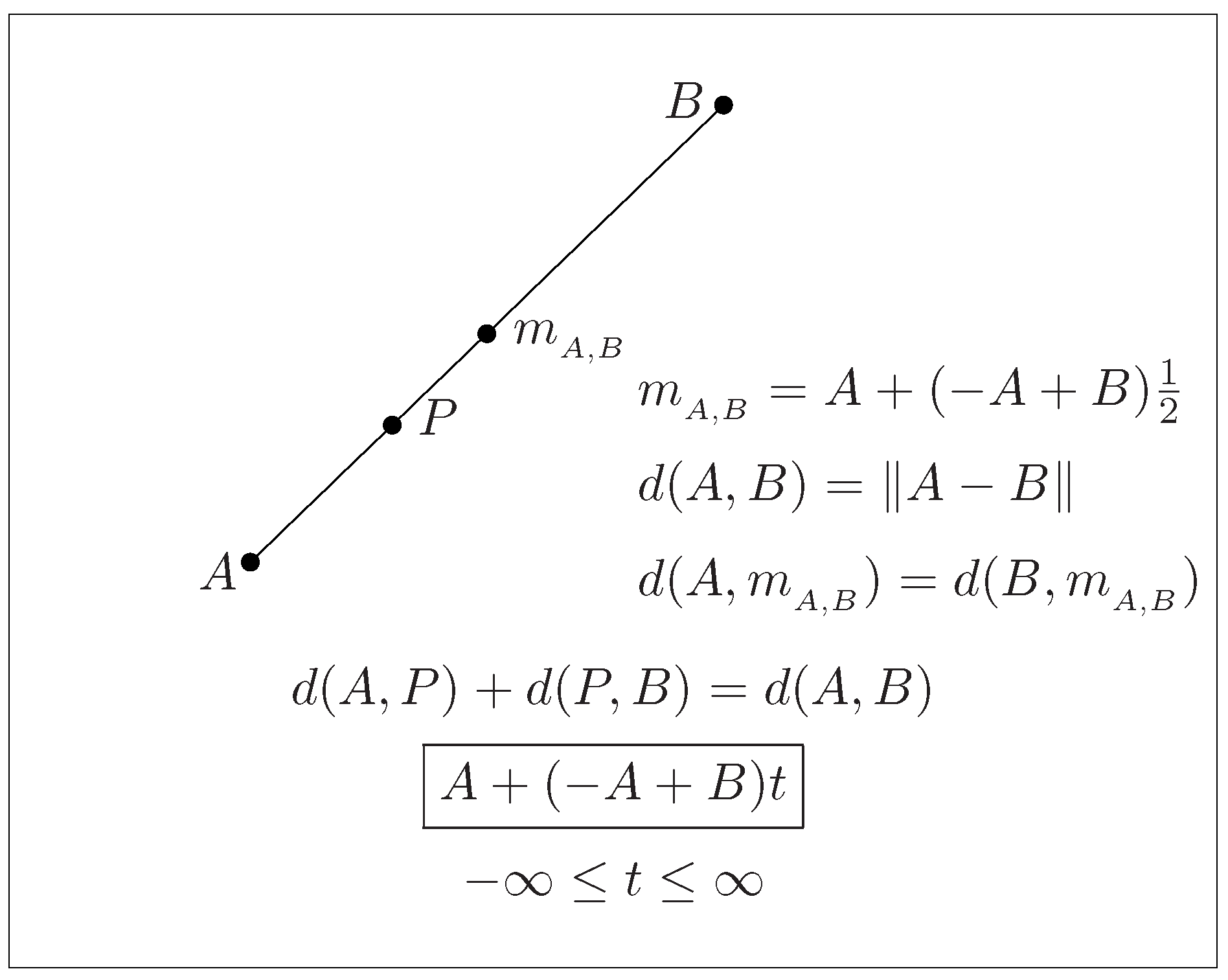
Figure 2.
Gyroline, the hyperbolic line. The gyroline LAB = A⊕(⊖A⊕B)⊗t, t ∈
, that passes through the points A and B in an Einstein gyrovector space (, ⊕, ⊗) is a geodesic line in the Beltrami-Klein ball model of hyperbolic geometry, fully analogous to the straight line A + (−A + B)t, t ∈
, in the Euclidean geometry of . The points A and B correspond to t = 0 and t = 1, respectively. The point P is a generic point on the gyroline through the points A and B lying between these points. The Einstein sum, ⊕, of the gyrodistance from A to P and from P to B equals the gyrodistance from A to B. The point mA,B is the gyromidpoint of the points A and B, corresponding to t = 1/2. The analogies between lines and gyrolines, as illustrated in Figure 1 and Figure 2, are obvious. The gyroline LAB approaches the boundary of at its boundary points EA and EB. The boundary points of gyroline LAB are determined by A and B in ([9], Section 5.9).

Figure 3.
Gyroangles share remarkable analogies with angles, allowing the use of the elementary trigonometric functions cos, sin, etc., in gyrotrigonometry as well. Let and be points different from O, lying arbitrarily on the gyrosegments and , respectively, that emanate from a common point O in an Einstein gyrovector space as shown here for . The measure of the gyroangle formed by the two gyrosegments and or, equivalently, formed by the two gyrosegments and , is given by , as shown here. In full analogy with angles, the measure of gyroangle is independent of the choice of and .

Figure 4.
Gyrotriangle , along with its standard notation, in an Einstein gyrovector space. The notation that we use with a gyrotriangle , its gyrovector sides, and its gyroangles in an Einstein gyrovector space is shown here for the Einstein gyrovector plane .
Figure 4.
Gyrotriangle , along with its standard notation, in an Einstein gyrovector space. The notation that we use with a gyrotriangle , its gyrovector sides, and its gyroangles in an Einstein gyrovector space is shown here for the Einstein gyrovector plane .

Figure 5.
Illustrating Ptolemy’s Theorem in the Euclidean plane. is a cyclic quadrilateral. It is inscribed in its circumcircle centered at its circumcenter O, with radius . The O-vertex angles , , and satisfy the equation . Ptolemy’s Theorem asserts that , where , . The hyperbolic counterpart of this figure is shown in Figure 6.

Figure 6.
Illustrating Ptolemy’s Theorem in the hyperbolic plane regulated by Einstein gyrovector plane . is a gyrocyclic gyroquadrilateral. It is inscribed in its circumgyrocircle gyrocentered at its circumgyrocenter O, with gyroradius . The O-gyrovertex gyroangles , , and satisfy the equation . The Hyperbolic Ptolemy’s Theorem is fully analogous to its Euclidean counterpart, asserting that , where , etc., is defined by (59) along with (48).

Figure 7.
A Gyrodiametric Gyrotriangle. The circumgyrocenter, O, of gyrotriangle is contained in gyroside of the gyrotriangle. Hence, the gyrotriangle is gyrodiametric, obeying the three equations that are shown in the Figure, where is the defect of gyrotriangle .
Figure 7.
A Gyrodiametric Gyrotriangle. The circumgyrocenter, O, of gyrotriangle is contained in gyroside of the gyrotriangle. Hence, the gyrotriangle is gyrodiametric, obeying the three equations that are shown in the Figure, where is the defect of gyrotriangle .

Disclaimer/Publisher’s Note: The statements, opinions and data contained in all publications are solely those of the individual author(s) and contributor(s) and not of MDPI and/or the editor(s). MDPI and/or the editor(s) disclaim responsibility for any injury to people or property resulting from any ideas, methods, instructions or products referred to in the content. |
© 2023 by the author. Licensee MDPI, Basel, Switzerland. This article is an open access article distributed under the terms and conditions of the Creative Commons Attribution (CC BY) license (https://creativecommons.org/licenses/by/4.0/).
Share and Cite
MDPI and ACS Style
Ungar, A.A. Ptolemy’s Theorem in the Relativistic Model of Analytic Hyperbolic Geometry. Symmetry 2023, 15, 649. https://doi.org/10.3390/sym15030649
AMA Style
Ungar AA. Ptolemy’s Theorem in the Relativistic Model of Analytic Hyperbolic Geometry. Symmetry. 2023; 15(3):649. https://doi.org/10.3390/sym15030649
Chicago/Turabian StyleUngar, Abraham A. 2023. "Ptolemy’s Theorem in the Relativistic Model of Analytic Hyperbolic Geometry" Symmetry 15, no. 3: 649. https://doi.org/10.3390/sym15030649
Note that from the first issue of 2016, this journal uses article numbers instead of page numbers. See further details here.