Traversable Wormhole Solutions Admitting Noether Symmetry in $f(\mathcal{R},{\mathcal{T}}^2)$ Theory

Abstract

This paper uses the Noether symmetry approach to examine the viable and stable traversable wormhole solutions in the framework of the $f(\mathcal{R},{\mathcal{T}}^2)$ theory, where $\mathcal{R}$ is the Ricci scalar and ${\mathcal{T}}^2={\mathcal{T}}_{\mu \nu }{\mathcal{T}}^{\mu \nu }$ is the self-contraction of the stress–energy tensor. For this purpose, we consider a specific model of this modified theory to obtain the exact solutions of the Noether equations. Further, we formulate the generators of the Noether symmetry and first integrals of motion. We analyze the presence of viable and stable traversable wormhole solutions corresponding to different redshift functions. In order to determine whether this theory provides physically viable and stable wormhole geometry or not, we check the graphical behavior of the null energy constraint, causality condition and adiabatic index for an effective stress–energy tensor. It is found that viable and stable traversable wormhole solutions exist in this modified theory.

1. Introduction

The general theory of relativity (GR) is the most effective theory of gravity which describes a wide range of gravitational effects from small to large structures in the cosmos. This theory passes the solar system tests successfully. Recent observations confirmed the existence of gravitational waves and showed that their power spectrum and attributes are consistent with those predicted by GR. The most comprehensive model for explaining the dynamics of the cosmos is the CDM model. However, the cosmological constant in the action of GR leads to the cosmological constant problem. However, there are many other unresolved issues such as the dark energy paradox and the existence of singularities which keep open the way to extend GR. It is fascinating that modifying GR can help in finding solutions for all these issues. $f(\mathcal{R})$ gravity is the simplest modified theory whose useful literature has been made available to comprehend the realistic aspects of this theory [1,2]. There are various modified gravitational theories that successfully describe the mysterious universe [3,4,5,6,7].

The prediction of singularities at a high energy level where GR is not applicable because of possible quantum effects is considered a significant issue in GR. However, quantum gravity does not have a specific formalism. Accordingly, a new gravitational theory has been established by adding the non-linear term ${\mathcal{T}}^{\mu \nu }{\mathcal{T}}_{\mu \nu }$ in the integral action, named $f(\mathcal{R},{\mathcal{T}}^2)$ gravity [8]. This theory is also equivalent to GR in a vacuum. This modified theory is assumed to be the most successful approach to resolve the spacetime singularity in the non-quantum description. This theory is also known as energy–momentum squared gravity (EMSG). Thus, the field equations of EMSG deviate from GR in the presence of a matter source. This theory includes higher-order matter and curvature terms in the field equations which are used to examine several interesting cosmic consequences. It is noteworthy that this modified proposal resolves the spacetime singularity, but cosmic evolution remains unaffected.

This mathematical model does not support the big-bang theory as the scale factor is minimum and the maximum energy density is finite in the early times. However, the density profile in the radiation-dominated era manifests that EMSG favors the inflationary cosmic models. These models resolve the main cosmic problems such as flatness and horizon issues, but no model of inflation has been confirmed by observations. A class of cosmic models (varying the speed of light theories) has been developed in this perspective which does not support the inflation. This suggested an alternative way to solve these cosmic problems by varying the speed of light and Newton’s constant of gravitation. Theories about varying the speed of light were motivated to resolve the inflation problems but did not resolve the big-bang singularity. To address this problem, Bhattacharjee and Sahoo [9] proposed a novel cosmic model which is free from inflation as well as the big-bang singularity by including Newton’s constant of gravitation and varying the speed of light in the context of EMSG. Singh et al. [10] studied the viability and stability of color-flavor locked quark stars in this framework. Nazari [11] examined that this theory passes the solar system tests successfully and found that, except for a small deviation, the behavior of light curves in EMSG is similar to GR.

The presence of the ${\mathcal{T}}^2$ term yields some quadratic corrections to the Friedman equations which are similar to those reported in the framework of loop quantum gravity [12]. Board and Barrow [13] analyzed a range of exact solutions for the isotropic universe and examined their behavior through accelerated expansion and the presence or absence of singularities. Akarsu et al. [14] proposed energy–momentum-powered gravity by adding the term $f({\mathcal{T}}_{\mu \nu }{\mathcal{T}}^{\mu \nu })$ in the functional action and discussed a specific case $f({\mathcal{T}}_{\mu \nu }{\mathcal{T}}^{\mu \nu })=\alpha {({\mathcal{T}}_{\mu \nu }{\mathcal{T}}^{\mu \nu })}^{\eta }$, where $\alpha$ and $\eta$ are real constants. They analyzed that this theory can be unified with Starobinsky gravity to explain the complete cosmic history, including the inflationary era. Akarsu et al. [15] established a scale-independent EMSG that leads to scenarios with many interesting applications in cosmology. Ranjit et al. [16] investigated solutions for matter density and studied their cosmic consequences in EMSG. Sharif and Naz [17] investigated viable features of a gravastar in this framework.

Chen and Chen [18] investigated the axial perturbations of the charged black holes in the EMSG theory. It is worthwhile to mention here that this theory is not limited to bouncing solutions and the early universe. However, this can be used to manipulate the CMB temperature fluctuation [19]. Kazemi et al. [20] analyzed the gravitational stability of an infinite fluid as well as the differentially rotating fluid in this framework. Rudra and Pourhassan [21] explored the thermodynamic properties of a black hole in EMSG. Nazari et al. [22] examined the Palatini formulation of EMSG and studied their consequences in various contexts. We have studied the stability of the Einstein universe [23,24] and dynamics of relativistic objects [25,26,27,28,29] in this framework. Yousaf et al. [30] analyzed the effects of EMSG on the dynamics of axially symmetric anisotropic and dissipative fluid. Khodadi and Firouzjaee [31] used the linear perturbations on the Reissner–Nordstrom–de Sitter solutions in this framework and developed the valid study of cosmic censorship conjecture beyond Einstein’s gravity.

The surprising and ambiguous characteristics of our cosmos put forward stunning questions for the scientific community. The existence of hypothetical structures is considered the most significant issue that gives the wormhole (WH) structure. It is described as a hypothetical bridge that connects two distinct parts of the universe due to the presence of exotic matter (which violates energy conditions). The intra-universe WH connects different regions of the same cosmos while the inter-universe WH joins two distinct parts of a different cosmos. Flamm [32] developed a WH structure through the Schwarzschild solution. Later, Einstein and Rosen [33] found that a curved space structure can join two different spacetimes through a bridge named the Einstein–Rosen bridge. Wheeler [34] explained the Schwarzschild WH is non-traversable because two-way traveling is not possible in it, and anything attempting to pass through would be destroyed by the tremendous tidal forces present at the WH throat. Moreover, the WH throat rapidly expands from zero to a finite circumference and compresses to zero with time, preventing access to anything. However, Fuller and Wheeler [35] investigated that WHs would collapse instantly after the formation.

The maximum amount of exotic matter in the bridge raises questions about the existence of a viable WH structure. Thus, there should not be an excessive amount of exotic matter in the bridge for viable WH geometry. The first traversable WH was proposed by Morris and Thorne [36]. In addition to the existence of such hypothetical structures, stability is the most significant issue that describes how these cosmic structures respond to perturbations and enhances their physical features. However, a stable state is obtained due to the non-singular configuration which prevents the WH from collapsing in contrast to an unstable WH, which can also exist because of very slow decay. Several methods were established to investigate the viable and stable WH structures [37,38]. Dzhunushaliev et al. [39] investigated the stability of a WH configuration with and without an electromagnetic field. Oliveira et al. [40] examined physically viable and stable traversable Yukawa–Casimir WHs.

Symmetry describes the properties of mathematical and physical systems that remain invariant due to perturbation. The uses of symmetry techniques are significant for obtaining viable solutions to differential systems. The continuous symmetry (which occurs due to constant change in a system) corresponding to the Lagrangian is known as Noether symmetry (NS). The associated Lagrangian is useful to identify the realistic aspects of a physical system by providing information about various symmetries of the system. However, the NS technique is the most elegant approach that describes a connection between NS generators and the conserved quantities of the system [41]. The complexity of the system is reduced by this method and viable solutions are obtained that can be used to study the dark cosmos. The literature provides several ways to explain the NS methodology [42,43,44]. For example, one way to identify the symmetry generators is with Noether gauge symmetry in which the gauge term is added to the invariance condition, while another method is to set the Lie derivative of the Lagrangian to zero. This technique also produces some useful restrictions that allow one to select cosmological models according to the recent observations [45,46,47].

Noether charges play a significant role as they are used to investigate several cosmic issues in various backgrounds. Motavali and Golshani [48] used the NS method to obtain the exact cosmological solutions of FRW spacetime. Vakili [49] used this approach to analyze dark components of the universe. Capozziello et al [50] analyzed this strategy in the quintessence and phantom cosmic models. Capozziello et al. [51,52] obtained viable solutions of static spherical spacetime through the NS method in $f(\mathcal{R})$ theory. Shamir et al. [53] obtained the exact solutions of the FRW universe model in the same theory. Jamil et al. [54] investigated scalar field cosmology through the NS approach in teleparallel theory. Momeni et al. [55] studied the exact cosmological solutions through NS in $f(\mathcal{R},\mathcal{T})$ theory. Shamir and Ahmad [56,57] examined isotropic and anisotropic solutions via the NS technique in $f(\mathcal{G},\mathcal{T})$ theory. We have found exact solutions through the NS technique in $f(\mathcal{R},{\mathcal{T}}^2)$ theory [58,59,60,61,62].

Cosmologists have been quite passionate about studying WH geometry in modified theories. Lobo et al. [63] examined a traversable WH structure through distinct types of WH shape functions (WSFs) and equations of state in $f(\mathcal{R})$ theory. Mazharimousavi and Halilsoy [64] found that WH solutions satisfy all the necessary requirements near the WH throat in this theory. In the framework of the scalar–tensor theory, the traversable WH geometry through the NS was examined in [65]. The static WH solutions with different matter contents in $f(\mathcal{R},\mathcal{T})$ theory were analyzed in [66]. The viable WH solutions admitting the NS in $f(\mathcal{R})$ theory were studied in [67]. Sharif et al. [68,69] studied a new holographic dark energy model and the Tsallis holographic dark energy model in the context of the modified theories of gravity. Mustafa et al. [70] analyzed viable WH geometry through the Karmarkar condition in $f(Q)$ theory. Shamir and Fayyaz [71] developed a WSF through the embedding class-I technique in $f(\mathcal{R})$ theory and explained that a WH structure can be obtained with a negligible amount of exotic matter. Hassan et al. [72] found that WH solutions corresponding to a linear and exponential model of $f(Q)$ gravity models are physically viable and stable. Malik et al. [73] used the Karmarkar condition to study a traversable WH structure in $f(\mathcal{R})$ theory.

The above literature motivates us to examine WH geometry through the NS approach in $f(\mathcal{R},{\mathcal{T}}^2)$ theory. This paper is designed in the following way. In Section 2, we develop the field equations of the static spherical spacetime in $f(\mathcal{R},{\mathcal{T}}^2)$ theory. Section 3 gives a brief discussion of WH solutions via the NS technique. In Section 4, we analyze the stability of the WH solutions by the causality condition and adiabatic index. The last section summarizes our results.

2. Basic Formalism of $\mathit{f}(\mathcal{R},{\mathcal{T}}^{\mathbf{2}})$ Theory

This modified theory is defined by the following action [8]

$$\mathcal{A}=\int (\frac{f(\mathcal{R},{\mathcal{T}}^2)}{2\kappa }+L_m)\sqrt{-g}{d}^{4}x,$$

(1)

where $L_m$, $\kappa$ and g represent the matter-Lagrangian, coupling constant and determinant of the line element, respectively. The corresponding field equations are

$$(g_{\mu \nu }{\nabla }_{\mu }{\nabla }^{\mu }+{\mathcal{R}}_{\mu \nu }-{\nabla }_{\mu }{\nabla }_{\mu })f_{\mathcal{R}}-\frac{1}{2}{g}_{\mu \nu }f={\mathcal{T}}_{\mu \nu }-{\Theta }_{\mu \nu }{f}_{{\mathcal{T}}^2},$$

(2)

where $f\equiv f(\mathcal{R},{\mathcal{T}}^2)$, $f_{{\mathcal{T}}^2}=\frac{\partial f}{\partial {\mathcal{T}}^2}$, $f_{\mathcal{R}}=\frac{\partial f}{\partial \mathcal{R}}$, and

$$\begin{array}{c}\hfill {\Theta }_{\mu \nu }=2{\mathcal{T}}_{\mu }^{\xi }{\mathcal{T}}_{\nu \xi }-\mathcal{T}{\mathcal{T}}_{\mu \nu }-2L_m{\mathcal{T}}_{\mu \nu }+L_m{g}_{\mu \nu }\mathcal{T}-\frac{4{\partial }^2{L}_m}{\partial g^{\mu \nu }\partial g^{\xi \eta }}{\mathcal{T}}^{\xi \eta }.\end{array}$$

(3)

We assume isotropic fluid configuration as

$${\mathcal{T}}_{\mu \nu }={\mathcal{U}}_{\mu }{\mathcal{U}}_{\nu }\rho +p({\mathcal{U}}_{\mu }{\mathcal{U}}_{\nu }+g_{\mu \nu }).$$

(4)

Using this value in Equation (3), we have

$$\begin{array}{c}\hfill {\Theta }_{\mu \nu }=-(4p\rho +{\rho }^2+3p^2){\mathcal{U}}_{\mu }{\mathcal{U}}_{\nu }.\end{array}$$

(5)

Re-arranging Equation (2), we obtain

$$G_{\mu \nu }=\frac{1}{f_{\mathcal{R}}}({\mathcal{T}}_{\mu \nu }^c+{\mathcal{T}}_{\mu \nu })={\mathcal{T}}_{\mu \nu }^{eff},$$

(6)

where ${\mathcal{T}}_{\mu \nu }^c$ are the additional impacts of EMSG, defined as

$${\mathcal{T}}_{\mu \nu }^c=\frac{1}{2}{g}_{\mu \nu }(f-\mathcal{R}{f}_{\mathcal{R}})+({\nabla }_{\mu }{\nabla }_{\nu }-g_{\mu \nu }{\nabla }_{\mu }{\nabla }^{\mu })f_{\mathcal{R}}-{\Theta }_{\mu \nu }{f}_{{\mathcal{T}}^2}.$$

(7)

We consider static spherical spacetime to study the WH geometry as [36]

$$d{s}^2=-d{t}^2{e}^{\alpha (r)}+d{r}^2{e}^{\beta (r)}+(d{\theta }^2+d{\varphi }^2{sin}^2\theta )\eta (r),$$

(8)

where $\eta (r)=sinhr$, $r^2$, $sinr$ for $K=-1,0,1$ (K defines the curvature parameter) [74]. We assume $e^{\beta (r)}={(1-\frac{h(r)}{r})}^{-1}$ and $\eta (r)=r^2$ to examine the WH structure. Here, $\alpha (r)$ and $h(r)$ define the redshift and WSF, respectively. Morris and Thorne [36] stated that the WSF must satisfy the following constraints in order to produce a traversable WH solution

$$\begin{array}{ccc}\hfill & & h(r)-r=0atr=r_0,\hfill \end{array}$$

(9)

$$\begin{array}{ccc}\hfill & & h^{\prime }(r)<1,\hfill \end{array}$$

(10)

$$\begin{array}{ccc}\hfill & & \frac{h(r)}{r}\to 0asr\to \infty ,\hfill \end{array}$$

(11)

$$\begin{array}{ccc}\hfill & & \frac{h(r)-rh{(r)}^{\prime }}{h{(r)}^2}>0atr=r_0.\hfill \end{array}$$

(12)

Here, $r_0$ is the radius of WH throat such that $r_0<r<\infty$. The resulting field equations are

$$\begin{array}{ccc}{\rho }^{eff}\hfill & =& \frac{1}{f_{\mathcal{R}}}[\rho +\frac{1}{2}(\mathcal{R}{f}_{\mathcal{R}}-f)+(3p^2+{\rho }^2+4p\rho )f_{{\mathcal{T}}^2}+e^{-\beta }(\frac{{\eta }^{\prime }}{\eta }-\frac{{\beta }^{\prime }}{2})f_{\mathcal{R}}^{\prime }\hfill \\ & +& e^{-\beta }{f}_{\mathcal{R}}^{″}],\hfill \end{array}$$

(13)

$$\begin{array}{ccc}\hfill p^{eff}& =& \frac{1}{f_{\mathcal{R}}}\left[p+\frac{1}{2}(f-\mathcal{R}{f}_{\mathcal{R}})-e^{-\beta }(\frac{{\eta }^{\prime }}{\eta }+\frac{{\alpha }^{\prime }}{2})f_{\mathcal{R}}^{\prime }\right].\hfill \end{array}$$

(14)

In order to analyze the existence of some viable cosmic structures, some constraints must be imposed on the matter, named energy conditions. These energy bounds are classified as follows:

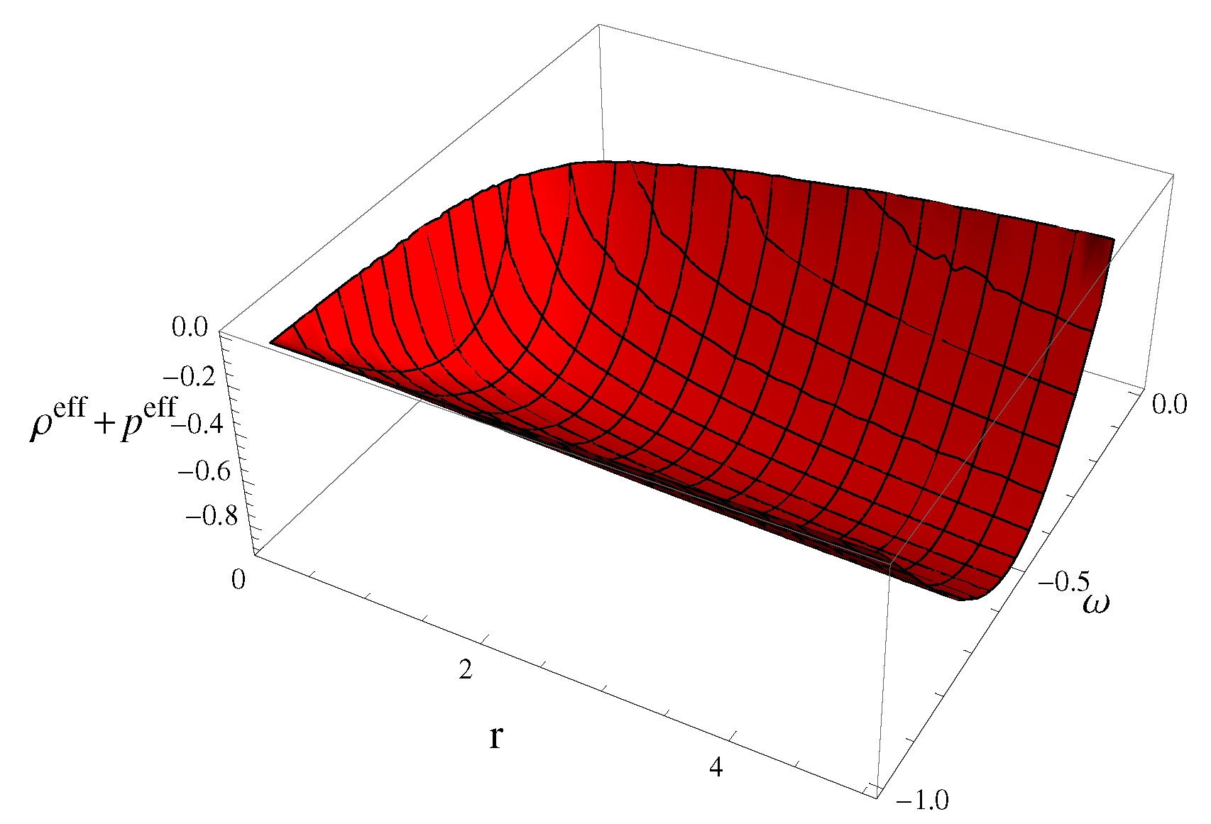
• Null energy constraint

  $$p^{eff}+{\rho }^{eff}\ge 0.$$

  (15)
• Strong energy constraint

  $$\begin{array}{c}\hfill p^{eff}+{\rho }^{eff}\ge 0,3p^{eff}+{\rho }^{eff}\ge 0.\end{array}$$

  (16)
• Dominant energy constraint

  $${\rho }^{eff}\pm p^{eff}\ge 0.$$

  (17)
• Weak energy constraint

  $$\begin{array}{c}\hfill p^{eff}+{\rho }^{eff}\ge 0,{\rho }^{eff}\ge 0.\end{array}$$

  (18)

These conditions must be violated for viable WH geometry. In alternative theories of gravity, the violation of $p^{eff}+{\rho }^{eff}\ge 0$ demonstrates the presence of a physically viable WH structure.

3. Noether Symmetry Approach

Noether symmetry offers an intriguing method for creating new cosmic models and associated structures in alternative gravitational theories. This method provides the first integrals of motion which are helpful to obtain exact solutions. We use Lagrange multiplier method as

$$S=2{\pi }^2\int \sqrt{-g}\left[f-(\mathcal{R}-\tilde{\mathcal{R}})v_1-({\mathcal{T}}^2-{\tilde{\mathcal{T}}}^2)v_2+p\right]dr,$$

(19)

where

$$\begin{array}{c}\hfill \sqrt{-g}=e^{\frac{\alpha +\beta }{2}}\eta ,{\tilde{\mathcal{T}}}^2=3p^2+{\rho }^2,v_1=f_{\mathcal{R}},v_2=f_{{\mathcal{T}}^2},\\ \hfill \tilde{\mathcal{R}}=-\frac{1}{e^{\beta }}\left({\alpha }^{″}+\frac{{{\eta }^{\prime }}^2}{2}+\frac{2{\eta }^{″}}{\eta }+\frac{{\alpha }^{\prime }{\eta }^{\prime }}{\eta }-\frac{{{\eta }^{\prime }}^2}{2{\eta }^2}-\frac{{\beta }^{\prime }{\eta }^{\prime }}{\eta }-\frac{{\alpha }^{\prime }{\beta }^{\prime }}{2}-\frac{2e^{\beta }}{\eta }\right).\end{array}$$

(20)

Using Equation (20) in (19), we obtain

$$\begin{array}{ccc}\hfill & & \mathcal{L}\left(\alpha ,\beta ,\eta ,\mathcal{R},{\mathcal{T}}^2,{\alpha }^{\prime },{\beta }^{\prime },{\eta }^{\prime },{\mathcal{R}}^{\prime },{({\mathcal{T}}^2)}^{\prime }\right)=\eta e^{\frac{\alpha +\beta }{2}}[f+p-f_{\mathcal{R}}(\mathcal{R}-2{\eta }^{-1})\hfill \\ \hfill & & +f_{{\mathcal{T}}^2}(3p^2+{\rho }^2-{\mathcal{T}}^2)]+\eta e^{\frac{\alpha -\beta }{2}}[(\frac{{\alpha }^{\prime }{\eta }^{\prime }}{\eta }+\frac{{{\eta }^{\prime }}^2}{2{\eta }^2})f_{\mathcal{R}}+(\frac{2{\eta }^{\prime }{\mathcal{R}}^{\prime }}{\eta }+{\alpha }^{\prime }{\mathcal{R}}^{\prime })f_{\mathcal{R}\mathcal{R}}\hfill \\ \hfill & & +(\frac{2{\eta }^{\prime }{({\mathcal{T}}^2)}^{\prime }}{\eta }+{\alpha }^{\prime }{({\mathcal{T}}^2)}^{\prime })f_{\mathcal{R}{\mathcal{T}}^2}].\hfill \end{array}$$

(21)

The Euler equations of motion and Hamiltonian of the system are expressed as

$$\begin{array}{ccc}\hfill & & \frac{\partial \mathcal{L}}{\partial q^i}-\frac{d}{dr}\left(\frac{\partial \mathcal{L}}{\partial q^{i^{\prime }}}\right)=0,i=1,2,3...,n\hfill \end{array}$$

(22)

$$\begin{array}{ccc}\hfill & & H=q^{i^{\prime }}\left(\frac{\partial \mathcal{L}}{\partial q^{i^{\prime }}}\right)-\mathcal{L},\hfill \end{array}$$

(23)

where generalized coordinates are denoted by $q^i$.

We use Lagrangian (21) in Equation (22) and obtain

$$\begin{array}{ccc}\hfill & & f-\mathcal{R}{f}_{\mathcal{R}}+p+f_{{\mathcal{T}}^2}(3p^2+{\rho }^2+12p{p}_{,\alpha }+4\rho {\rho }_{,\alpha }-{\mathcal{T}}^2)+2p_{,\alpha }-\frac{1}{e^{\beta }}\hfill \\ \hfill & & \times [\left(\frac{2{\eta }^{″}}{\eta }-\frac{{{\eta }^{\prime }}^2}{2{\eta }^2}-\frac{{\beta }^{\prime }{\eta }^{\prime }}{\eta }-\frac{2e^{\beta }}{\eta }\right)f_{\mathcal{R}}+\left(2{\mathcal{R}}^{″}-{\beta }^{\prime }{\mathcal{R}}^{\prime }+\frac{2{\eta }^{\prime }{\mathcal{R}}^{\prime }}{\eta }\right)f_{\mathcal{R}\mathcal{R}}\hfill \\ \hfill & & +\left(2{({\mathcal{T}}^2)}^{″}-{\beta }^{\prime }{({\mathcal{T}}^2)}^{\prime }+\frac{2{\eta }^{\prime }{({\mathcal{T}}^2)}^{\prime }}{\eta }\right)f_{\mathcal{R}{\mathcal{T}}^2}+2{{\mathcal{R}}^{\prime }}^2{f}_{\mathcal{R}\mathcal{R}\mathcal{R}}+4{\mathcal{R}}^{\prime }{({\mathcal{T}}^2)}^{\prime }{f}_{\mathcal{R}\mathcal{R}{\mathcal{T}}^2}\hfill \\ \hfill & & +2{({({\mathcal{T}}^2)}^{\prime })}^2{f}_{\mathcal{R}{\mathcal{T}}^2{\mathcal{T}}^2}]=0,\hfill \end{array}$$

(24)

$$\begin{array}{ccc}\hfill & & f-\mathcal{R}{f}_{\mathcal{R}}+p+f_{{\mathcal{T}}^2}(3p^2+{\rho }^2+12p{p}_{,\beta }+4\rho {\rho }_{,\beta }-{\mathcal{T}}^2)+2p_{,\beta }+\frac{1}{e^{\beta }}\hfill \\ \hfill & & \times [\left(\frac{2e^{\beta }}{\eta }-\frac{{{\eta }^{\prime }}^2}{2{\eta }^2}-\frac{{\alpha }^{\prime }{\eta }^{\prime }}{\eta }\right)f_{\mathcal{R}}-\left({\alpha }^{\prime }{\mathcal{R}}^{\prime }+\frac{2{\eta }^{\prime }{\mathcal{R}}^{\prime }}{\eta }\right)f_{\mathcal{R}\mathcal{R}}-{\alpha }^{\prime }{({\mathcal{T}}^2)}^{\prime }{f}_{\mathcal{R}{\mathcal{T}}^2}\hfill \\ \hfill & & -\frac{2{\eta }^{\prime }{({\mathcal{T}}^2)}^{\prime }}{\eta }{f}_{\mathcal{R}{\mathcal{T}}^2}]=0,\hfill \end{array}$$

(25)

$$\begin{array}{ccc}\hfill & & f-\mathcal{R}{f}_{\mathcal{R}}+f_{{\mathcal{T}}^2}(3p^2+{\rho }^2+6\eta p{p}_{,\eta }+2\eta \rho {\rho }_{,\eta }-{\mathcal{T}}^2)-\frac{1}{e^{\beta }}[({\alpha }^{″}+\frac{{{\alpha }^{\prime }}^2}{2}\hfill \\ \hfill & & +\frac{{\eta }^{″}}{\eta }+\frac{{\alpha }^{\prime }{\eta }^{\prime }}{2\eta }-\frac{{\beta }^{\prime }{\eta }^{\prime }}{2\eta }-\frac{{\alpha }^{\prime }{\beta }^{\prime }}{2}-\frac{{{\eta }^{\prime }}^2}{2{\eta }^2})f_{\mathcal{R}}+2{{\mathcal{R}}^{\prime }}^2{f}_{\mathcal{R}\mathcal{R}\mathcal{R}}+4{\mathcal{R}}^{\prime }{({\mathcal{T}}^2)}^{\prime }{f}_{\mathcal{R}\mathcal{R}{\mathcal{T}}^2}\hfill \\ \hfill & & +\left({\alpha }^{\prime }{\mathcal{R}}^{\prime }-{\beta }^{\prime }{\mathcal{R}}^{\prime }+2{\mathcal{R}}^{″}+\frac{{\eta }^{\prime }{\mathcal{R}}^{\prime }}{\eta }\right)f_{\mathcal{R}\mathcal{R}}+\left({\alpha }^{\prime }{({\mathcal{T}}^2)}^{\prime }-{\beta }^{\prime }({\mathcal{T}}^2)+2{({\mathcal{T}}^2)}^{″}\right.\hfill \\ \hfill & & \left.+\frac{{\eta }^{\prime }{({\mathcal{T}}^2)}^{\prime }}{\eta }\right)f_{\mathcal{R}{\mathcal{T}}^2}+2{({({\mathcal{T}}^2)}^{\prime })}^2{f}_{\mathcal{R}{\mathcal{T}}^2{\mathcal{T}}^2}-p{e}^{\beta }-\eta p_{,\eta }{e}^{\beta }]=0,\hfill \end{array}$$

(26)

$$\begin{array}{ccc}\hfill & & +e^{\beta }(\mathcal{R}-2{\eta }^{-1})f_{\mathcal{R}\mathcal{R}}-e^{\beta }(3p^2+{\rho }^2-{\mathcal{T}}^2)f_{\mathcal{R}{\mathcal{T}}^2}+[{\alpha }^{″}+\frac{{{\alpha }^{\prime }}^2}{2}+\frac{2{\eta }^{″}}{\eta }\hfill \\ \hfill & & +\frac{{\alpha }^{\prime }{\eta }^{\prime }}{\eta }-\frac{{\beta }^{\prime }{\eta }^{\prime }}{\eta }-\frac{{\alpha }^{\prime }{\beta }^{\prime }}{2}-\frac{{{\eta }^{\prime }}^2}{2{\eta }^2}]f_{\mathcal{R}\mathcal{R}}=0,\hfill \end{array}$$

(27)

$$\begin{array}{ccc}\hfill & & e^{\beta }(\mathcal{R}-2{\eta }^{-1})f_{\mathcal{R}{\mathcal{T}}^2}-e^{\beta }(3p^2+{\rho }^2-{\mathcal{T}}^2)f_{{\mathcal{T}}^2{\mathcal{T}}^2}+[{\alpha }^{″}+\frac{{{\alpha }^{\prime }}^2}{2}+\frac{2{\eta }^{″}}{\eta }\hfill \\ \hfill & & +\frac{{\alpha }^{\prime }{\eta }^{\prime }}{\eta }-\frac{{\beta }^{\prime }{\eta }^{\prime }}{\eta }-\frac{{\alpha }^{\prime }{\beta }^{\prime }}{2}-\frac{{{\eta }^{\prime }}^2}{2{\eta }^2}]f_{\mathcal{R}{\mathcal{T}}^2}=0.\hfill \end{array}$$

(28)

Using Equation (21) in (23), it follows

$$e^{\beta (r)}=\frac{\left(\frac{{{\eta }^{\prime }}^2}{2{\eta }^2}+\frac{{\alpha }^{\prime }{\eta }^{\prime }}{\eta }\right)f_{\mathcal{R}}+\left({\alpha }^{\prime }+\frac{2{\eta }^{\prime }}{\eta }\right)\left({\mathcal{R}}^{\prime }{f}_{\mathcal{R}\mathcal{R}}+{({\mathcal{T}}^2)}^{\prime }{f}_{{\mathcal{T}}^2{\mathcal{T}}^2}\right)}{\left(f-\mathcal{R}{f}_{\mathcal{R}}+\left(3p^2+{\rho }^2-{\mathcal{T}}^2\right)f_{{\mathcal{T}}^2}+p+\frac{2f_{\mathcal{R}}}{\eta }\right)}.$$

(29)

The symmetry generators are considered as

$$\mathcal{K}=\lambda \frac{\partial }{\partial r}+{\gamma }^i\frac{\partial }{\partial q^i},i=1,2,3,4,5.$$

(30)

where $\lambda =\lambda (\alpha ,\beta ,\eta ,\mathcal{R},{\mathcal{T}}^2)$ and $\gamma =\gamma (\alpha ,\beta ,\eta ,\mathcal{R},{\mathcal{T}}^2)$ are unknown coefficients of the vector field. For the existence of NS, the Lagrangian must satisfy the following invariance constraint

$${\mathcal{K}}^{\left[1\right]}\mathcal{L}+(D\lambda )\mathcal{L}=D\Psi ,$$

(31)

where total derivative, prolongation of first order and boundary term are represented by D, ${\mathcal{K}}^{\left[1\right]}$ and $\Psi$, respectively. Further, it is determined as

$${\mathcal{K}}^{\left[1\right]}=\mathcal{K}+{{\gamma }^i}^{\prime }\frac{\partial }{\partial {q^i}^{\prime }},D=\frac{\partial }{\partial r}+{q^i}^{\prime }\frac{\partial }{\partial q^i}.$$

(32)

Here, ${{\gamma }^i}^{\prime }=D{{\gamma }^i}^{\prime }-{q^i}^{\prime }D\lambda$. The conserved quantities are expressed as

$$I=-\lambda H+{\gamma }^i\frac{\partial \mathcal{L}}{\partial q^i}-\Psi ,$$

(33)

which play an important role for developing the viable solutions. The coefficients of Equation (31) are given in Appendix A.

4. Exact Solutions

This section formulates the symmetry generators, conserved quantities and corresponding viable solutions using the above system of PDEs. The system’s complexity decreases via the NS technique, which also helps to find the exact solutions. Thus, it would be interesting to study viable and traversable WH solutions using this approach. However, the aforementioned system is more complex, so it is very difficult to find exact solutions without taking the EMSG model. We assume the EMSG model as [12]

$$\mathcal{R}+\chi {\mathcal{T}}^2=f(\mathcal{R},{\mathcal{T}}^2).$$

(34)

where we take constant $\chi =1$ for our convenience. We include cosmological constant in this model to make the resemblance with the standard $\Lambda$CDM model as

$$\mathcal{R}+\Lambda ({\mathcal{T}}^2)+{\mathcal{T}}^2=f(\mathcal{R},{\mathcal{T}}^2).$$

(35)

The exact solutions of the system of Equations (A1)–(A19) are

$$\begin{array}{ccc}\hfill & & {\gamma }^2=-\frac{2{\xi }_2{\xi }_5}{r^2},\lambda ={\xi }_1-\frac{{\xi }_2{\xi }_5}{r},{\gamma }^1={\gamma }^3={\gamma }^4={\gamma }^5=0,\hfill \\ \hfill & & \Lambda ({\mathcal{T}}^2)=-{\mathcal{T}}^2+{\xi }_3{\mathcal{T}}^2+{\xi }_4,\Psi ={\xi }_{5}r,\hfill \end{array}$$

(36)

where arbitrary constants are denoted by ${\xi }_i$. It is important to consider isotropic matter because it accurately explains the composition of matter in various celestial objects. Dust fluid can also analyze the configuration of matter only in the presence of negligible amount of radiation. Here, we examine the existence of viable traversable WH structures for dust and non-dust fluid configurations.

4.1. Dust Case

Equation (4) becomes

$${\mathcal{T}}_{\mu \nu }=\rho {\mathcal{U}}_{\mu }{\mathcal{U}}_{\nu }.$$

(37)

Using Equation (37) in (A20), we have

$$\begin{array}{c}\hfill \rho =\sqrt{\frac{e^{\frac{-\alpha -\beta }{2}}}{2{\xi }_2{\xi }_3}},\mathcal{R}+2{\xi }_3{\mathcal{T}}^2+{\xi }_4=f(\mathcal{R},{\mathcal{T}}^2).\end{array}$$

(38)

The NS generators and corresponding first integrals of motion become

$$\begin{array}{ccc}\hfill {\mathcal{K}}_1& =& \frac{\partial }{\partial r},{\mathcal{K}}_2=-\frac{2{\xi }_2}{r}\frac{\partial }{\partial r}-\frac{2{\xi }_2}{r^2}\frac{\partial }{\partial \beta },\hfill \end{array}$$

(39)

$$\begin{array}{ccc}\hfill I_1& =& 2e^{\frac{\alpha -\beta }{2}}\left[1+{\alpha }^{\prime }r-\left(1+\frac{{\xi }_4{r}^2}{2}+\frac{r^2{e}^{\frac{-\alpha -\beta }{2}}}{2{\xi }_2}\right)e^{\beta }\right],\hfill \end{array}$$

(40)

$$\begin{array}{ccc}\hfill I_2& =& r-\frac{2{\xi }_2{e}^{\frac{\alpha -\beta }{2}}}{r}\left[1+{\alpha }^{\prime }r-\left(1+\frac{{\xi }_4{r}^2}{2}+\frac{r^2{e}^{\frac{-\alpha -\beta }{2}}}{2{\xi }_2}\right)e^{\beta }\right].\hfill \end{array}$$

(41)

Substituting Equation (38) in (29), we obtain

$$e^{\beta (r)}=\frac{1+{\alpha }^{\prime }r}{1+\frac{r^2{\xi }_4}{2}+\frac{r^2{e}^{\frac{-\alpha -\beta }{2}}}{2{\xi }_2}}.$$

(42)

We consider different redshift functions as [75,76]

$$\begin{array}{c}\hfill \alpha (r)=jln(\frac{r}{r_0}),\alpha (r)=e^{-\frac{r_0}{r}},\end{array}$$

(43)

to examine the viable WH geometry through null energy condition and WSF. Here, j is an arbitrary constant. We manipulate Equation (42) for the considered redshift functions in the following cases.

Case I:

$\alpha (r)=jln(\frac{r}{r_0})$

Substituting this value in (42), it follows

$$\begin{array}{ccc}\hfill \beta (r)& =& 4ln(2)-2ln\left[\frac{1}{{\xi }_2(r+j)}\right\{r^2+\{8{(\frac{r}{r_0})}^j{\xi }_2^2{\xi }_{4}j{r}^2+8{(\frac{r}{r_0})}^j{\xi }_2^2{\xi }_4{r}^3\hfill \\ \hfill & +& 16{(\frac{r}{r_0})}^j{\xi }_2^{2}j+16{(\frac{r}{r_0})}^j{\xi }_2^{2}r+r^4{\}}^{\frac{1}{2}}\left\}{(\frac{r}{r_0})}^{-j/2}\right].\hfill \end{array}$$

(44)

The corresponding WSF is

$$\begin{array}{ccc}\hfill h(r)& =& -\frac{r}{8{\xi }_2^2{(r+j)}^2}[4{\xi }_2^2{\xi }_{4}j{r}^2+4{\xi }_2^2{\xi }_4{r}^3+{(\frac{r}{r_0})}^{-j}{r}^4+{(\frac{r}{r_0})}^{-j}\{8j{r}^2{\xi }_2^2\hfill \\ \hfill & \times & {(\frac{r}{r_0})}^j{\xi }_4+8{(\frac{r}{r_0})}^j{\xi }_2^2{\xi }_4{r}^3+16{(\frac{r}{r_0})}^j{\xi }_2^{2}j+16{(\frac{r}{r_0})}^j{\xi }_2^{2}r+r^4{r}^2{\}}^{\frac{1}{2}}\hfill \\ \hfill & -& 8{\xi }_2^2{j}^2-16{\xi }_2^{2}jr-8{\xi }_2^2{r}^2+8{\xi }_2^{2}j+8{\xi }_2^{2}r].\hfill \end{array}$$

(45)

The energy density becomes

$$\begin{array}{ccc}\hfill \rho & =& \frac{\sqrt{2}}{4}\left[\frac{1}{{\xi }_2^2(r+j){\xi }_3}\right\{r^2+\{8{(\frac{r}{r_0})}^j{\xi }_2^2{\xi }_{4}j{r}^2+8{(\frac{r}{r_0})}^j{\xi }_2^2{\xi }_4{r}^3+16{(\frac{r}{r_0})}^j{\xi }_2^{2}j\hfill \\ \hfill & +& 16{(\frac{r}{r_0})}^j{\xi }_2^{2}r+r^4{\}}^{\frac{1}{2}}\}{(\frac{r}{r_0})}^{-j}{]}^{\frac{1}{2}}.\hfill \end{array}$$

(46)

The null energy condition turns out to be

$$\begin{array}{ccc}\hfill {\rho }^{eff}+p^{eff}& =& \frac{\sqrt{2}}{4}\left[\frac{1}{{\xi }_2^2(r+j){\xi }_3}\right\{r^2+\{8{(\frac{r}{r_0})}^j{\xi }_2^2{\xi }_{4}j{r}^2+8{(\frac{r}{r_0})}^j{\xi }_2^2{\xi }_4{r}^3+16j\hfill \\ \hfill & \times & {(\frac{r}{r_0})}^j{\xi }_2^2+16{(\frac{r}{r_0})}^j{\xi }_2^{2}r+r^4{\}}^{\frac{1}{2}}\}{(\frac{r}{r_0})}^{-j}{]}^{\frac{1}{2}}+\frac{1}{4}[\frac{1}{{\xi }_2^2(r+j)}\{r^2\hfill \\ \hfill & +& \{8{(\frac{r}{r_0})}^j{\xi }_2^2{\xi }_{4}j{r}^2+8{(\frac{r}{r_0})}^j{\xi }_2^2{\xi }_4{r}^3+16{(\frac{r}{r_0})}^j{\xi }_2^{2}j+16{(\frac{r}{r_0})}^j{\xi }_2^{2}r\hfill \\ \hfill & +& r^4{\}}^{\frac{1}{2}}\left\}{(\frac{r}{r_0})}^{-j}\right].\hfill \end{array}$$

(47)

We investigate the graphical behavior of WSF in Figure 1. In the upper panel, the left graph shows that the behavior of WSF is positive with $h(r)<r$, whereas the right graph represents asymptotically flat behavior, i.e., $h(r)\to 0$ when $r\to \infty$. The WH throat exists at $r_0=0.001$ and $\frac{dh(r_0)}{dr}<1$ as shown in the below panel of left and right graphs, respectively. The last plot shows that flaring-out condition is satisfied at wormhole throat. The graphical behavior of the null energy condition is given in Figure 2, which shows that the effective fluid variables violate null energy condition $({\rho }^{eff}+p^{eff}\le 0$), hence ensuring the presence of traversable WH geometry.

Case II:

$\alpha (r)=e^{\frac{r_0}{r}}$

Here, Equation (42) gives

$$\begin{array}{ccc}\hfill \beta (r)& =& 2ln\left[\frac{1}{4{\xi }_2}\right\{r^3+\{8{(e^{\frac{1}{2}{(e^{\frac{r_0}{r}})}^{-1}})}^2{\xi }_2^2{\xi }_4{r}^5+8e^{-\frac{1}{2}\frac{1}{r}(2r_0{e}^{\frac{r_0}{r}}-r){(e^{\frac{r_0}{r}})}^{-1}}{e}^{\frac{1}{2}{(e^{\frac{r_0}{r}})}^{-1}}\hfill \\ \hfill & \times & {\xi }_2^2{\xi }_4{r}_0{r}^3+16{(e^{\frac{1}{2}{(e^{\frac{r_0}{r}})}^{-1}})}^2{\xi }_2^2{r}^3+16e^{-\frac{1}{2}\frac{1}{r}(2r_0{e}^{\frac{r_0}{r}}-r){(e^{\frac{r_0}{r}})}^{-1}}{e}^{\frac{1}{2}{(e^{\frac{r_0}{r}})}^{-1}}{\xi }_2^2{r}_{0}r\hfill \\ \hfill & +& r^6{\}}^{\frac{1}{2}}\left\}{\left\{e^{\frac{1}{2}{(e^{\frac{r_0}{r}})}^{-1}}{r}^2+e^{-\frac{1}{2}\frac{1}{r}(2r_0{e}^{\frac{r_0}{r}}-r){(e^{\frac{r_0}{r}})}^{-1}}{r}_0\right\}}^{-1}\right].\hfill \end{array}$$

(48)

The corresponding WSF becomes

$$\begin{array}{ccc}\hfill b(r)& =& [1-16{\xi }_2^2{\left\{e^{\frac{1}{2}{(e^{\frac{r_0}{r}})}^{-1}}{r}^2+e^{-\frac{1}{2}\frac{1}{r}(2r_0{e}^{\frac{r_0}{r}}-r){(e^{\frac{r_0}{r}})}^{-1}}{r}_0\right\}}^2[r^3+\{{(e^{\frac{1}{2}{(e^{\frac{r_0}{r}})}^{-1}})}^2\hfill \\ \hfill & \times & 8{\xi }_2^2{\xi }_4{r}^5+8e^{-\frac{1}{2}\frac{1}{r}(2r_0{e}^{\frac{r_0}{r}}-r){(e^{\frac{r_0}{r}})}^{-1}}{e}^{\frac{1}{2}{(e^{\frac{r_0}{r}})}^{-1}}{\xi }_2^2{\xi }_4{r}_0{r}^3+16{(e^{\frac{1}{2}{(e^{\frac{r_0}{r}})}^{-1}})}^2{\xi }_2^2{r}^3\hfill \\ \hfill & +& 16e^{-\frac{1}{2}\frac{1}{r}(2r_0{e}^{\frac{r_0}{r}}-r){(e^{\frac{r_0}{r}})}^{-1}}{e}^{\frac{1}{2}{(e^{\frac{r_0}{r}})}^{-1}}{\xi }_2^2{r}_{0}r+r^6{\}}^{\frac{1}{2}}{]}^{-2}]r.\hfill \end{array}$$

(49)

The energy density in this case is given as

$$\begin{array}{ccc}\hfill \rho & =& \sqrt{2}\left[\frac{e^{-\frac{1}{2}{e}^{-\frac{r_0}{r}}}}{{\xi }_3}\left\{e^{1/2e^{-\frac{r_0}{r}}}{r}^2+e^{-1/2\frac{1}{r}(2r_0{e}^{\frac{r_0}{r}}-r)e^{-\frac{r_0}{r}}}{r}_0\right\}\right[r^3+\{r(8e^{e^{-\frac{r_0}{r}}}{\xi }_2^2{\xi }_4{r}^4\hfill \\ \hfill & +& 8e^{-\frac{1}{r}{e}^{-\frac{r_0}{r}}(r_0{e}^{\frac{r_0}{r}}-r)}{\xi }_2^2{\xi }_4{r}_0{r}^2+16e^{e^{-\frac{r_0}{r}}}{\xi }_2^2{r}^2+r^5+e^{-\frac{1}{r}{e}^{-\frac{r_0}{r}}}(r_0{e}^{\frac{r_0}{r}}-r)\hfill \\ \hfill & \times & 16{\xi }_2^2{r}_0){\}}^{\frac{1}{2}}{]}^{-1}{]}^{\frac{1}{2}}.\hfill \end{array}$$

(50)

Substituting the value of redshift function and $\beta (r)$ in Equations (13) and (14), we have

$$\begin{array}{ccc}\hfill {\rho }^{eff}+p^{eff}& =& \sqrt{2}\left[\frac{e^{-\frac{1}{2}{e}^{-\frac{r_0}{r}}}}{{\xi }_3}\left\{e^{\frac{1}{2}{e}^{-\frac{r_0}{r}}}{r}^2+e^{-\frac{1}{2}\frac{1}{r}(2r_0{e}^{\frac{r_0}{r}}-r)e^{-\frac{r_0}{r}}}{r}_0\right\}\right[r^3+\{r(8r^4\hfill \\ \hfill & \times & e^{e^{-\frac{r_0}{r}}}{\xi }_2^2{\xi }_4+8e^{-\frac{1}{r}{e}^{-\frac{r_0}{r}}(r_0{e}^{\frac{r_0}{r}}-r)}{\xi }_2^2{\xi }_4{r}_0{r}^2+16e^{e^{-\frac{r_0}{r}}}{\xi }_2^2{r}^2+r^5+{\xi }_2^2{r}_0\hfill \\ \hfill & \times & 16e^{-\frac{1}{r}{e}^{-\frac{r_0}{r}}}(r_0{e}^{\frac{r_0}{r}}-r)){\}}^{\frac{1}{2}}{]}^{-1}{]}^{\frac{1}{2}}+{\xi }_3[\frac{e^{-1/2e^{-\frac{r_0}{r}}}}{{\xi }_3}\{e^{\frac{1}{2}{e}^{-\frac{r_0}{r}}}{r}^2\hfill \\ \hfill & +& e^{-1/2\frac{1}{r}(2r_0{e}^{\frac{r_0}{r}}-r)e^{-\frac{r_0}{r}}}{r}_0\left\}\right[r^3+\{r(8e^{e^{-\frac{r_0}{r}}}{\xi }_2^2{\xi }_4{r}^4+e^{-\frac{1}{r}{e}^{-\frac{r_0}{r}}(r_0{e}^{\frac{r_0}{r}}-r)}\hfill \\ \hfill & \times & 8{\xi }_2^2{\xi }_4{r}_0{r}^2+16e^{e^{-\frac{r_0}{r}}}{\xi }_2^2{r}^2+r^5+e^{-\frac{1}{r}{e}^{-\frac{r_0}{r}}}(r_0{e}^{\frac{r_0}{r}}-r)\hfill \\ \hfill & \times & 16{\xi }_2^2{r}_0){\}}^{\frac{1}{2}}{]}^{-1}].\hfill \end{array}$$

(51)

In Figure 3, the upper right plot determines that the behavior of shape function is not asymptotically flat while left plot implies that $h(r)<r$. The right plot in the below panel shows $\frac{dh(r_0)}{dr}<1$ and the left plot determines that WH throat exists at $r_0=0.01$. Moreover, the flaring-out condition satisfies at wormhole throat. Figure 4 violates the null energy condition which manifests the existence of viable traversable WH geometry.

4.2. Non-Dust Case

Here, we assume a specific relation between fluid parameters as $p=\omega \rho$ ($\omega$ is EoS parameter) and manipulate Equation (A20) which gives

$$\rho =\frac{-{\xi }_2\omega +\sqrt{{\xi }_2^2{\omega }^2+4{\xi }_2{\xi }_3{e}^{\frac{-\alpha -\beta }{2}}+12{\xi }_2{\xi }_3{\omega }^2{e}^{\frac{-\alpha -\beta }{2}}}}{2{\xi }_2{\xi }_3(3{\omega }^2+1)}.$$

(52)

The NS generators and the corresponding integral of motion yield

$$\begin{array}{ccc}\hfill {\mathcal{K}}_1& =& \frac{\partial }{\partial r},{\mathcal{K}}_2=-\frac{2{\xi }_2}{r}\frac{\partial }{\partial r}-\frac{2{\xi }_2}{r^2}\frac{\partial }{\partial \beta },\hfill \end{array}$$

(53)

$$\begin{array}{ccc}\hfill I_1& =& e^{\frac{\alpha -\beta }{2}}{r}^2[2(\frac{1+{\alpha }^{\prime }r}{r^2})-e^{\beta }\left({\xi }_4+\frac{2}{r^2}+\left({\xi }_3\left(3{\omega }^2+1\right)\right)\right.\hfill \\ \hfill & \times & {\left(\frac{-{\xi }_2\omega +\sqrt{{\xi }_2^2{\omega }^2+4{\xi }_2{\xi }_3{e}^{\frac{-\alpha -\beta }{2}}+12{\xi }_2{\xi }_3{\omega }^2{e}^{\frac{-\alpha -\beta }{2}}}}{2{\xi }_2{\xi }_3\left(3{\omega }^2+1\right)}\right)}^2\hfill \\ \hfill & +& \left.\omega \frac{-{\xi }_2\omega +\sqrt{{\xi }_2^2{\omega }^2+4{\xi }_2{\xi }_3{e}^{\frac{-\alpha -\beta }{2}}+12{\xi }_2{\xi }_3{\omega }^2{e}^{\frac{-\alpha -\beta }{2}}}}{2{\xi }_2{\xi }_3\left(3{\omega }^2+1\right)}\right)],\hfill \\ \hfill I_2& =& r-{\xi }_{2}r{e}^{\frac{\alpha -\beta }{2}}[\frac{2{\alpha }^{\prime }}{r}+\frac{2}{r^2}-e^{\beta }\left({\xi }_4+\frac{2}{r^2}+\left({\xi }_3\left(3{\omega }^2+1\right)\right)\right.\hfill \\ \hfill & \times & {\left(\frac{-{\xi }_2\omega +\sqrt{{\xi }_2^2{\omega }^2+4{\xi }_2{\xi }_3{e}^{\frac{-\alpha -\beta }{2}}+12{\xi }_2{\xi }_3{\omega }^2{e}^{\frac{-\alpha -\beta }{2}}}}{2{\xi }_2{\xi }_3\left(3{\omega }^2+1\right)}\right)}^2\hfill \end{array}$$

(54)

$$\begin{array}{ccc}\hfill & +& \left.\omega \frac{-{\xi }_2\omega +\sqrt{{\xi }_2^2{\omega }^2+4{\xi }_2{\xi }_3{e}^{\frac{-\alpha -\beta }{2}}+12{\xi }_2{\xi }_3{\omega }^2{e}^{\frac{-\alpha -\beta }{2}}}}{2{\xi }_2{\xi }_3\left(3{\omega }^2+1\right)}\right)].\hfill \end{array}$$

(55)

Using Equation (52) in (29), we have

$$e^{\beta (r)}=\frac{2+2{\alpha }^{\prime }r}{r^2\left({\xi }_4+\frac{2}{r^2}+\frac{e^{\frac{-\alpha -\beta }{2}}}{{\xi }_2}\right)}.$$

(56)

Now, we examine the presence of viable WH geometry for the identical redshift functions that were studied in the dust case.

Case I:

$\alpha (r)=jln(\frac{r}{r_0})$

Equation (56) in this case turns out to be

$$\begin{array}{ccc}\hfill \beta (r)& =& 4ln(2)-2ln\left[\frac{1}{{\xi }_2(r+j)}\right\{r^2+\{8{(\frac{r}{r_0})}^j{\xi }_2^2{\xi }_{4}j{r}^2+8{(\frac{r}{r_0})}^j{\xi }_2^2{\xi }_4{r}^3\hfill \\ \hfill & +& 16j{(\frac{r}{r_0})}^j{\xi }_2^2+16{(\frac{r}{r_0})}^j{\xi }_2^{2}r+r^4{\}}^{\frac{1}{2}}\left\}{(\frac{r}{r_0})}^{-\frac{j}{2}}\right].\hfill \end{array}$$

(57)

The WSF becomes

$$\begin{array}{ccc}\hfill b(r)& =& -\frac{r}{8{\xi }_2^2{(r+j)}^2}[4{\xi }_2^2{\xi }_{4}j{r}^2+4{\xi }_2^2{\xi }_4{r}^3+{(\frac{r}{r_0})}^{-j}{r}^4+{(\frac{r}{r_0})}^{-j}\{8{(\frac{r}{r_0})}^j\hfill \\ \hfill & \times & {\xi }_2^2{\xi }_{4}j{r}^2+8{(\frac{r}{r_0})}^j{\xi }_2^2{\xi }_4{r}^3+16{(\frac{r}{r_0})}^j{\xi }_2^{2}j+16{(\frac{r}{r_0})}^j{\xi }_2^{2}r+r^4{r}^2{\}}^{\frac{1}{2}}\hfill \\ \hfill & -& 8{\xi }_2^2{j}^2-16{\xi }_2^{2}jr-8{\xi }_2^2{r}^2+8{\xi }_2^{2}j+8{\xi }_2^{2}r].\hfill \end{array}$$

(58)

Substituting Equation (57) in (52), we obtain

$$\begin{array}{ccc}\hfill \rho & =& \frac{1}{2{\xi }_2{\xi }_3(3{\omega }^2+1)}[-{\xi }_2\omega +\{\frac{1}{r+j}(3{\omega }^2{\xi }_3{(\frac{r}{r_0})}^{-j}{r}^2+3{(\frac{r}{r_0})}^{-j}(8{(\frac{r}{r_0})}^j\hfill \\ \hfill & \times & {\xi }_2^2{c}_{4}j{r}^2+8{(\frac{r}{r_0})}^j{\xi }_2^2{c}_4{r}^3+16{(\frac{r}{r_0})}^j{\xi }_2^{2}j+16{(\frac{r}{r_0})}^j{\xi }_2^{2}r+r^4{)}^{\frac{1}{2}}{\xi }_3{\omega }^2\hfill \\ \hfill & +& {\xi }_3{(\frac{r}{r_0})}^{-j}{r}^2+{\xi }_2^2{\omega }^{2}j+{\xi }_2^2{\omega }^{2}r+{(\frac{r}{r_0})}^{-j}(8{(\frac{r}{r_0})}^j{\xi }_2^2{c}_{4}j{r}^2+8{(\frac{r}{r_0})}^j{\xi }_2^2{c}_4{r}^3\hfill \\ \hfill & +& 16{(\frac{r}{r_0})}^j{\xi }_2^{2}j+16{(\frac{r}{r_0})}^j{\xi }_2^{2}r+r^4{)}^{\frac{1}{2}}{\xi }_3){\}}^{\frac{1}{2}}].\hfill \end{array}$$

(59)

Figure 5 manifests that WH geometry is asymptotically flat and shape function maintains its positivity. The right graph in the lower panel indicates that $\frac{dh(r_0)}{dr}<1$, and the associated left graph shows that WH throat exists at $r_0=0.01$. The last plot shows that flaring-out condition satisfied at wormhole throat in this case. The corresponding null energy condition turns out to be

$$\begin{array}{ccc}\hfill {\rho }^{eff}+p^{eff}& =& (1+\omega )\left[\frac{1}{2{\xi }_2{\xi }_3(3{\omega }^2+1)}\right[-{\xi }_2\omega +\{\frac{1}{r+j}(3{\omega }^2{\xi }_3{(\frac{r}{r_0})}^{-j}{r}^2\hfill \\ \hfill & +& 3{(\frac{r}{r_0})}^{-j}(8{(\frac{r}{r_0})}^j{\xi }_2^2{c}_{4}j{r}^2+8{(\frac{r}{r_0})}^j{\xi }_2^2{c}_4{r}^3+16{(\frac{r}{r_0})}^j{\xi }_2^{2}j+16r\hfill \\ \hfill & \times & {(\frac{r}{r_0})}^j{\xi }_2^2+r^4{)}^{\frac{1}{2}}{\xi }_3{\omega }^2+{\xi }_3{(\frac{r}{r_0})}^{-j}{r}^2+{\xi }_2^2{\omega }^{2}j+{\xi }_2^2{\omega }^{2}r+{(\frac{r}{r_0})}^{-j}\hfill \\ \hfill & \times & (8{(\frac{r}{r_0})}^j{\xi }_2^2{c}_{4}j{r}^2+8{(\frac{r}{r_0})}^j{\xi }_2^2{c}_4{r}^3+16{(\frac{r}{r_0})}^j{\xi }_2^{2}j+16{(\frac{r}{r_0})}^j{\xi }_2^{2}r\hfill \\ \hfill & +& r^4{)}^{\frac{1}{2}}{\xi }_3){\}}^{\frac{1}{2}}]]+2{\xi }_3({\omega }^2+4\omega +1)[\frac{1}{2{\xi }_2{\xi }_3(3{\omega }^2+1)}[-{\xi }_2\omega \hfill \\ \hfill & +& \{\frac{1}{r+j}(3{\omega }^2{\xi }_3{(\frac{r}{r_0})}^{-j}{r}^2+3{(\frac{r}{r_0})}^{-j}(8{(\frac{r}{r_0})}^j{\xi }_2^2{c}_{4}j{r}^2+8{(\frac{r}{r_0})}^j\hfill \\ \hfill & \times & {\xi }_2^2{c}_4{r}^3+16{(\frac{r}{r_0})}^j{\xi }_2^{2}j+16{(\frac{r}{r_0})}^j{\xi }_2^{2}r+r^4{)}^{\frac{1}{2}}{\xi }_3{\omega }^2+{\xi }_3{(\frac{r}{r_0})}^{-j}{r}^2\hfill \\ \hfill & +& {\xi }_2^2{\omega }^{2}j+{\xi }_2^2{\omega }^{2}r+{(\frac{r}{r_0})}^{-j}(8{(\frac{r}{r_0})}^j{\xi }_2^2{c}_{4}j{r}^2+8{(\frac{r}{r_0})}^j{\xi }_2^2{c}_4{r}^3\hfill \\ \hfill & +& 16{(\frac{r}{r_0})}^j{\xi }_2^{2}j+16{(\frac{r}{r_0})}^j{\xi }_2^{2}r+r^4{)}^{\frac{1}{2}}{\xi }_3){\}}^{\frac{1}{2}}]{]}^2.\hfill \end{array}$$

(60)

Figure 6 shows that viable traversable WH exists in the specific range of EoS parameter.

Case II:

$\alpha (r)=e^{-\frac{r_0}{r}}$

Here, Equation (59) leads to

$$\begin{array}{ccc}\hfill \beta (r)& =& 2ln\left[\frac{1}{4{\xi }_2}\right\{r^3+\{8{(e^{1/2{(e^{\frac{r_0}{r}})}^{-1}})}^2{\xi }_2^2{\xi }_4{r}^5+8e^{-1/2\frac{1}{r}(2r_0{e}^{\frac{r_0}{r}}-r){(e^{\frac{r_0}{r}})}^{-1}}{e}^{1/2{(e^{\frac{r_0}{r}})}^{-1}}\hfill \\ \hfill & \times & {\xi }_2^2{\xi }_4{r}_0{r}^3+16{(e^{1/2{(e^{\frac{r_0}{r}})}^{-1}})}^2{\xi }_2^2{r}^3+16e^{-1/2\frac{1}{r}(2r_0{e}^{\frac{r_0}{r}}-r){(e^{\frac{r_0}{r}})}^{-1}}{e}^{1/2{(e^{\frac{r_0}{r}})}^{-1}}{\xi }_2^2{r}_{0}r\hfill \\ \hfill & +& r^6{\}}^{\frac{1}{2}}\left\}{\left\{e^{1/2{(e^{\frac{r_0}{r}})}^{-1}}{r}^2+e^{-1/2\frac{1}{r}(2r_0{e}^{\frac{r_0}{r}}-r){(e^{\frac{r_0}{r}})}^{-1}}{r}_0\right\}}^{-1}\right].\hfill \end{array}$$

(61)

The corresponding WSF is

$$\begin{array}{ccc}\hfill h(r)& =& [1-16{\xi }_2^2{\left\{e^{1/2{(e^{\frac{r_0}{r}})}^{-1}}{r}^2+e^{-1/2\frac{1}{r}(2r_0{e}^{\frac{r_0}{r}}-r){(e^{\frac{r_0}{r}})}^{-1}}{r}_0\right\}}^2[r^3+\{8{\xi }_2^2{\xi }_4{r}^5\hfill \\ \hfill & \times & {(e^{1/2{(e^{\frac{r_0}{r}})}^{-1}})}^2+8e^{-1/2\frac{1}{r}(2r_0{e}^{\frac{r_0}{r}}-r){(e^{\frac{r_0}{r}})}^{-1}}{e}^{1/2{(e^{\frac{r_0}{r}})}^{-1}}{\xi }_2^2{\xi }_4{r}_0{r}^3+16{\xi }_2^2{r}^3\hfill \\ \hfill & \times & {(e^{1/2{(e^{\frac{r_0}{r}})}^{-1}})}^2+16e^{-1/2\frac{1}{r}(2r_0{e}^{\frac{r_0}{r}}-r){(e^{\frac{r_0}{r}})}^{-1}}{e}^{1/2{(e^{\frac{r_0}{r}})}^{-1}}{\xi }_2^2{r}_{0}r\hfill \\ \hfill & +& r^6{\}}^{\frac{1}{2}}{]}^{-2}]r.\hfill \end{array}$$

(62)

Figure 7 determines that WSF is positive with $h(r)<r$, but the behavior of wormhole is not asymptotically flat. The WH throat is located at $r_0=0.001$ with $\frac{dh(r_0)}{dr}<1$. The flaring-out condition is fulfilled at wormhole throat. The energy density turns out to be

$$\begin{array}{ccc}\hfill \rho & =& \frac{1}{2{\xi }_2{\xi }_3(3{\omega }^2+1)}[-{\xi }_2\omega +[{\xi }_2^2\{48{\xi }_3{\omega }^2{r}^2+48{\xi }_3{r}_0{\omega }^2{e}^{-\frac{r_0}{r}}+16{\xi }_3{r}^2\hfill \\ \hfill & +& {\omega }^2{r}^3+16{\xi }_3{r}_0{e}^{-\frac{r_0}{r}}+\{r(8e^{e^{-\frac{r_0}{r}}}{\xi }_2^2{\xi }_4{r}^4+8e^{-\frac{1}{r}{e}^{-\frac{r_0}{r}}(r_0{e}^{\frac{r_0}{r}}-r)}{\xi }_2^2{\xi }_4{r}_0{r}^2\hfill \\ \hfill & +& 16e^{e^{-\frac{r_0}{r}}}{\xi }_2^2{r}^2+r^5+16e^{-\frac{1}{r}{e}^{-\frac{r_0}{r}}(r_0{e}^{\frac{r_0}{r}}-r)}{\xi }_2^2{r}_0){\}}^{\frac{1}{2}}{\omega }^2\}\{r^3+\{r(8r^4\hfill \\ \hfill & \times & e^{e^{-\frac{r_0}{r}}}{\xi }_2^2{\xi }_4+8{\xi }_2^2{\xi }_4{r}_0{r}^2{e}^{-\frac{1}{r}{e}^{-\frac{r_0}{r}}(r_0{e}^{\frac{r_0}{r}}-r)}+16e^{e^{-\frac{r_0}{r}}}{\xi }_2^2{r}^2+r^5+16{\xi }_2^2{r}_0\hfill \\ \hfill & \times & e^{-\frac{1}{r}{e}^{-\frac{r_0}{r}}(r_0{e}^{\frac{r_0}{r}}-r)}){\}}^{\frac{1}{2}}{\}}^{-1}{]}^{\frac{1}{2}}].\hfill \end{array}$$

(63)

The null energy condition yields

$$\begin{array}{ccc}\hfill {\rho }^{eff}+p^{eff}& =& (1+\omega )\left[\frac{1}{2{\xi }_2{\xi }_3(3{\omega }^2+1)}\right[-{\xi }_2\omega +\left[{\xi }_2^2\right\{48{\xi }_3{\omega }^2{r}^2+48{\xi }_3{r}_0{\omega }^2{e}^{-\frac{r_0}{r}}\hfill \\ \hfill & +& 16{\xi }_3{r}^2+{\omega }^2{r}^3+16{\xi }_3{r}_0{e}^{-\frac{r_0}{r}}+\{r(8e^{e^{-\frac{r_0}{r}}}{\xi }_2^2{\xi }_4{r}^4+8e^{-\frac{1}{r}{e}^{-\frac{r_0}{r}}(r_0{e}^{\frac{r_0}{r}}-r)}\hfill \\ \hfill & \times & {\xi }_2^2{\xi }_4{r}_0{r}^2+16e^{e^{-\frac{r_0}{r}}}{\xi }_2^2{r}^2+r^5+16e^{-\frac{1}{r}{e}^{-\frac{r_0}{r}}(r_0{e}^{\frac{r_0}{r}}-r)}{\xi }_2^2{r}_0){\}}^{\frac{1}{2}}{\omega }^2\}\{r^3\hfill \\ \hfill & +& \{r(8e^{e^{-\frac{r_0}{r}}}{\xi }_2^2{\xi }_4{r}^4+8{\xi }_2^2{\xi }_4{r}_0{r}^2{e}^{-\frac{1}{r}{e}^{-\frac{r_0}{r}}(r_0{e}^{\frac{r_0}{r}}-r)}+16e^{e^{-\frac{r_0}{r}}}{\xi }_2^2{r}^2+r^5\hfill \\ \hfill & +& 16e^{-\frac{1}{r}{e}^{-\frac{r_0}{r}}(r_0{e}^{\frac{r_0}{r}}-r)}{\xi }_2^2{r}_0){\}}^{\frac{1}{2}}{\}}^{-1}{]}^{\frac{1}{2}}]]+2{\xi }_3(3{\omega }^2+4\omega +1)\hfill \\ \hfill & \times & \left[\frac{1}{2{\xi }_2{\xi }_3(3{\omega }^2+1)}\right[-{\xi }_2\omega +\left[{\xi }_2^2\right\{48{\xi }_3{\omega }^2{r}^2+48{\xi }_3{r}_0{\omega }^2{e}^{-\frac{r_0}{r}}+16{\xi }_3{r}^2\hfill \\ \hfill & +& {\omega }^2{r}^3+16{\xi }_3{r}_0{e}^{-\frac{r_0}{r}}+\{r(8e^{e^{-\frac{r_0}{r}}}{\xi }_2^2{\xi }_4{r}^4+8e^{-\frac{1}{r}{e}^{-\frac{r_0}{r}}(r_0{e}^{\frac{r_0}{r}}-r)}{\xi }_2^2{\xi }_4{r}_0{r}^2\hfill \\ \hfill & +& 16e^{e^{-\frac{r_0}{r}}}{\xi }_2^2{r}^2+r^5+16e^{-\frac{1}{r}{e}^{-\frac{r_0}{r}}(r_0{e}^{\frac{r_0}{r}}-r)}{\xi }_2^2{r}_0){\}}^{\frac{1}{2}}{\omega }^2\}\{r^3+\{r(8r^4\hfill \\ \hfill & \times & e^{e^{-\frac{r_0}{r}}}{\xi }_2^2{\xi }_4+8{\xi }_2^2{\xi }_4{r}_0{r}^2{e}^{-\frac{1}{r}{e}^{-\frac{r_0}{r}}(r_0{e}^{\frac{r_0}{r}}-r)}+16e^{e^{-\frac{r_0}{r}}}{\xi }_2^2{r}^2+r^5+16{\xi }_2^2{r}_0\hfill \\ \hfill & \times & e^{-\frac{1}{r}{e}^{-\frac{r_0}{r}}(r_0{e}^{\frac{r_0}{r}}-r)}){\}}^{\frac{1}{2}}{\}}^{-1}{]}^{\frac{1}{2}}]{]}^2.\hfill \end{array}$$

(64)

The graphical behavior of effective matter variables is given in Figure 8 which shows that traversable WH exists in this modified theory for $-1\le \omega \le 0$.

5. Stability Analysis

In order to analyze the valid and consistent cosmic structures, stability is significant. It is more interesting to examine cosmic objects that display stable behavior under the external perturbations. In the following, we investigate the stable WH solutions via the causality condition and adiabatic index.

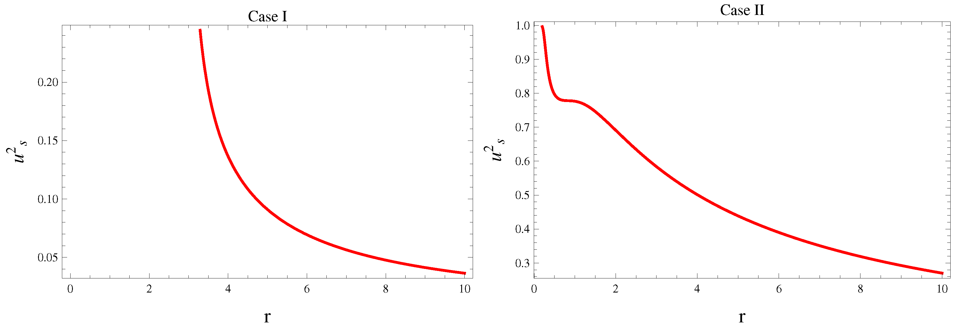
5.1. Causality Condition

A stable stellar system is considered more viable in the realm of gravitational physics. When the system experiences non-disappearing forces, it is important to observe how the matter variables behave after disruption from the equilibrium condition. The causality condition is a mathematical requirement that imposes constraints on the system. In the context of a stability analysis, the causality condition is used to check whether a system is stable or not. If the system satisfies the causality condition, it means that the corresponding system is stable and that the output will not exhibit any oscillations or instability. Here, we use the causality condition to check the stable state of WH solutions. According to this condition, the square speed of sound $(u_s^2=\frac{d{p}^{eff}}{d{\rho }^{eff}})$ should satisfy the limit, $0\le u_s^2<1$ [77].

However, outside this region of stability, the output of the system may exhibit different forms of instability. For example, if the function violates the causality condition, it may give rise to an unstable system, and that exhibits oscillations or even divergent behavior. In some cases, the instability may be in the form of noise or other unwanted behavior that can make the system unusable for its intended purpose. Another form of instability that can occur outside the region of stability is related to the Nyquist stability criterion. This criterion is based on the mapping of the frequency response of the function onto the complex plane. If the Nyquist plot encircles the point (–1, 0) in a clockwise direction, the system is unstable. This instability can manifest itself as oscillations or other types of unwanted behavior. Hence, while the causality condition is an important requirement for stability, it is not the only factor that determines whether a system is stable or not. Other forms of instability can occur outside the region of stability, and these may require different methods for analysis and control. Figure 9 and Figure 10 show that WH solutions satisfy the required causality condition in the presence of modified terms.

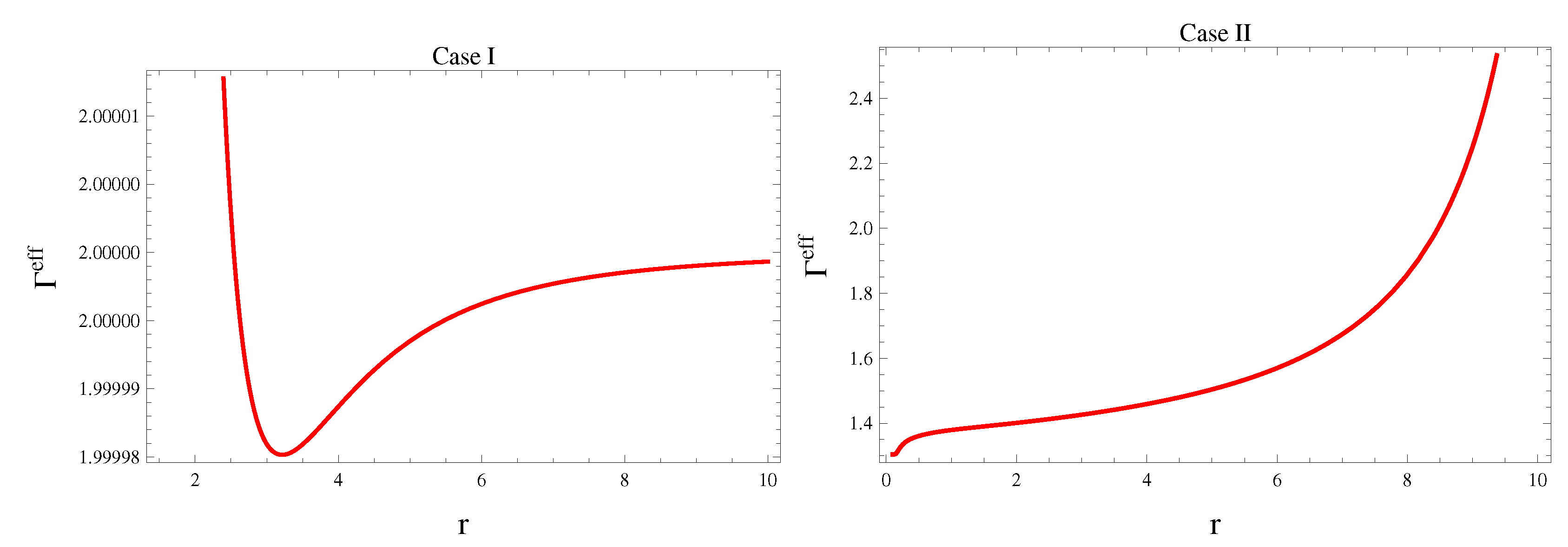
5.2. Adiabatic Index

This is an alternative technique to explore the stability of celestial objects. The adiabatic index, also known as the gamma factor, is a measure of the thermodynamic properties of a gas and is defined as the ratio of the specific heat at constant pressure to the specific heat at constant volume. In the context of astrophysics, the adiabatic index is used to determine the stability of a star against the radial perturbation. A star is said to be stable if it can resist small radial oscillations without undergoing a collapse or explosion. The adiabatic index is related to the speed of sound in the stellar material, and a lower value of the adiabatic index indicates a softer material and a higher value indicates a stiffer material. For a stable star, the adiabatic index must be greater than a critical value, typically around 4/3 [78]. The adiabatic index depends on the composition of the stellar material, which in turn affects the nuclear reactions that take place in the star’s core. As a star burns through its fuel, the composition of its material changes, and this can affect the star’s adiabatic index and stability. Therefore, the adiabatic index is an important parameter in the study of stellar structure and evolution, and it is used to understand the behavior of stars and their compositions. Many researchers used this condition in the literature [79,80,81,82,83,84,85].

The adiabatic index is expressed as

$${\Gamma }^{eff}=\frac{p^{eff}+{\rho }^{eff}}{p^{eff}}{u}_s^2.$$

(65)

According to Heintzmann and Hillebrandt [78], a system is stable if $\Gamma >4/3$, otherwise it is unstable. Figure 11 and Figure 12 show that WH solutions satisfy the required limits in both (dust and non-dust) cases, indicating that our system is in a stable state.

6. Final Remarks

The existence of a WH structure is a crucial issue in the field of astrophysics. In GR, the existence of exotic matter is significant for the presence of physically realistic WH geometry. In the last few decades, the scientific community has paid a lot of attention to modified theories of gravity as a possible alternative to GR. Many scientists found these modified theories interesting when used to analyze the viable traversable WH geometry due to the violation of energy bounds by the effective stress-energy tensor which ensures the presence of a viable WH structure.

In this manuscript, we have used the NS approach to find some exact solutions that help to formulate static WH solutions in $f(\mathcal{R},{\mathcal{T}}^2)$ theory. We have examined the existence of exotic matter in WHs via the violation of the null energy condition. For different matter configurations, we have investigated the viable WH geometry corresponding to different redshift functions, i.e., $\alpha (r)=jln(\frac{r}{r_0})$ and $\alpha (r)=e^{-\frac{r_0}{r}}$. Finally, we have investigated the stability of the obtained WH solutions through the causality condition and adiabatic index. We have examined NS generators and conserved quantities corresponding to both dust and non-dust cases. The summary of the obtained results is given as follows.

• For $\alpha (r)=jln(\frac{r}{r_0})$, it is found that the WSF satisfies all the required conditions and preserves the asymptotically flat behavior for both the dust and dust matter configurations (Figure 1 and Figure 5).
• The wormhole shape function does not preserve the asymptotically flat behavior for $\alpha (r)=e^{-\frac{r_0}{r}}$ (Figure 3 and Figure 7).
• For the dust matter configuration, the effective energy–momentum tensor violates the null energy condition for both choices of redshift functions that show the existence of traversable WH geometry in $f(\mathcal{R},{\mathcal{T}}^2)$ theory (Figure 2 and Figure 4).
• In the non-dust case, we have found that ${\rho }^{eff}+p^{eff}\le 0$ for a specific range of the EoS parameter which indicates the existence of a viable and traversable WH (Figure 6 and Figure 8).
• It is found that traversable WHs are stable for both types of the redshift function in the presence of modified terms (Figure 9, Figure 10, Figure 11 and Figure 12).

In the framework of GR, Fayyaz and Shamir [85] studied physically realistic and stable WH solutions in the presence of exotic matter. The same authors [71] found that the considered WSF satisfies the null energy condition and hence shows the absence of exotic matter which yields non-traversable WH geometry in $f(\mathcal{R})$ theory. We have found that the null energy condition is violated in the context of the $f(\mathcal{R},{\mathcal{T}}^2)$ theory, which shows that viable and stable traversable WH solutions exist in this modified theory.

References

1. De Felice, A.; Tsujikawa, S. f(R) theories. Living Rev. Relativ. 2010, 13, 1–161. [Google Scholar] [CrossRef] [PubMed] [Green Version]
2. Nojiri, S.I.; Odintsov, S.D. Unified cosmic history in modified gravity: From F(R) theory to Lorentz non-invariant models. Phys. Rep. 2011, 505, 59–144. [Google Scholar] [CrossRef] [Green Version]
3. Harko, T.; Lobo, F.S.; Nojiri, S.I.; Odintsov, S.D. f(R,T) gravity. Phys. Rev. D 2011, 84, 024020. [Google Scholar] [CrossRef] [Green Version]
4. Sharif, M.; Gul, M.Z. Study of charged spherical collapse in f(G,T) gravity. Eur. Phys. J. Plus 2018, 133, 345. [Google Scholar] [CrossRef]
5. Sharif, M.; Gul, M.Z. Dynamics of cylindrical collapse in f(G,T) gravity. Chin. J. phys. 2019, 57, 329–337. [Google Scholar] [CrossRef]
6. Sharif, M.; Gul, M.Z. Dynamics of perfect fluid collapse in f(G,T) gravity. Int. J. Mod. Phys. D 2019, 28, 1950054. [Google Scholar] [CrossRef]
7. Sharif, M.; Gul, M.Z. Stellar structures admitting Noether symmetries in f(R,T) gravity. Mod. Phys. Lett. A 2021, 36, 2150214. [Google Scholar] [CrossRef]
8. Katirci, N.; Kavuk, M. Gravity and Cardassian-like expansion as one of its consequences. Eur. Phys. J. Plus 2014, 129, 163. [Google Scholar] [CrossRef]
9. Bhattacharjee, S.; Sahoo, P.K. Temporally varying universal gravitational constant and speed of light in energy-momentum squared gravity. Eur. Phys. J. Plus 2020, 135, 86. [Google Scholar] [CrossRef]
10. Singh, K.N.; Banerjee, A.; Maurya, S.K.; Rahaman, F.; Pradhan, A. Color-flavor locked quark stars in energy-momentum squared gravity. Phys. Dark Universe 2021, 31, 100774. [Google Scholar] [CrossRef]
11. Nazari, E. Light bending and gravitational lensing in energy-momentum-squared gravity. Phys. Rev. D 2022, 105, 104026. [Google Scholar] [CrossRef]
12. Roshan, M.; Shojai, F. Energy-momentum squared gravity. Phys. Rev. D 2016, 94, 044002. [Google Scholar] [CrossRef] [Green Version]
13. Board, C.V.; Barrow, J.D. Cosmological models in energy-momentum-squared gravity. Phys. Rev. D 2017, 96, 123517. [Google Scholar] [CrossRef] [Green Version]
14. Akarsu, O.; Katirci, N.; Kumar, S. Cosmic acceleration in a dust only Universe via energy-momentum powered gravity. Phys. Rev. D 2018, 2018 97, 024011. [Google Scholar] [CrossRef] [Green Version]
15. Akarsu, O.; Katirci, N.; Kumar, S.; Nunes, R.C.; Sami, M. Cosmological implications of scale-independent energy-momentum squared gravity: Pseudo nonminimal interactions in dark matter and relativistic relics. Phys. Rev. D 2018, 98, 063522. [Google Scholar] [CrossRef] [Green Version]
16. Ranjit, C.; Rudra, P.; Kundu, S. Constraints on Energy-Momentum Squared Gravity from cosmic chronometers and Supernovae Type Ia data. Ann. Phys. 2021, 428, 168432. [Google Scholar] [CrossRef]
17. Sharif, M.; Naz, S. Gravastars with Karmarkar condition in f(R,T2) gravity. Int. J. Mod. Phys. D 2022, 31, 2240008. [Google Scholar] [CrossRef]
18. Chen, C.Y.; Chen, P. Eikonal black hole ringings in generalized energy-momentum squared gravity. Phys. Rev. D 2020, 101, 064021. [Google Scholar] [CrossRef] [Green Version]
19. Akarsu, O.; Barrow, J.D.; Uzun, N.M. Screening anisotropy via energy-momentum squared gravity: ΛCDM model with hidden anisotropy. Phys. Rev. D 2020, 102, 124059. [Google Scholar] [CrossRef]
20. Kazemi, A.; Roshan, M.; De Martino, I.; De Laurentis, M. Jeans analysis in energy-momentum-squared gravity. Eur. Phys. J. C 2020, 80, 150. [Google Scholar] [CrossRef]
21. Rudra, P.; Pourhassan, B. Thermodynamics of the apparent horizon in the generalized energy-momentum-squared cosmology. Phys. Dark Universe 2021, 33, 100849. [Google Scholar] [CrossRef]
22. Nazari, E.; Sarvi, F.; Roshan, M. Generalized energy-momentum-squared gravity in the Palatini formalism. Phys. Rev. D 2020, 102, 064016. [Google Scholar] [CrossRef]
23. Sharif, M.; Gul, M.Z. Stability of the closed Einstein universe in energy-momentum squared gravity. Phys. Scr. 2021, 96, 105001. [Google Scholar] [CrossRef]
24. Sharif, M.; Gul, M.Z. Effects of f(R,T2) gravity on the stability of anisotropic perturbed Einstein Universe. Pramana J. Phys. 2022, 96, 153. [Google Scholar] [CrossRef]
25. Sharif, M.; Gul, M.Z. Dynamics of spherical collapse in energy-momentum squared gravity. Int. J. Mod. Phys. A 2021, 36, 2150004. [Google Scholar] [CrossRef]
26. Gul, M.Z.; Sharif, M. Dynamical analysis of charged dissipative cylindrical collapse in energy-momentum squared gravity. Universe 2021, 7, 154. [Google Scholar] [CrossRef]
27. Sharif, M.; Gul, M.Z. Study of stellar structures in f(R,TμνTμν) theory. Int. J. Geom. Methods Mod. Phys. 2022, 19, 2250012. [Google Scholar] [CrossRef]
28. Sharif, M.; Gul, M.Z. Dynamics of charged anisotropic spherical collapse in energy-momentum squared gravity. Chin. J. Phys. 2021, 71, 365–374. [Google Scholar] [CrossRef]
29. Sharif, M.; Gul, M.Z. Role of energy-momentum squared gravity on the dynamics of charged dissipative plane symmetric collapse. Mod. Phys. Lett. A 2022, 37, 2250005. [Google Scholar] [CrossRef]
30. Yousaf, Z.; Bhatti, M.Z.; Farwa, U. Evolution of axially and reflection symmetric source in energy-momentum squared gravity. Eur. Phys. J. Plus 2022, 137, 1–22. [Google Scholar] [CrossRef]
31. Khodadi, M.; Firouzjaee, J.T. A survey of strong cosmic censorship conjecture beyond Einstein’s gravity. Phys. Dark Universe 2022, 37, 101084. [Google Scholar] [CrossRef]
32. Flamm, L. Beitrge zur Einsteinschen gravitationstheorie. Phys. Z. 1916, 17, 448–454. [Google Scholar]
33. Einstein, A.; Rosen, N. The particle problem in the general theory of relativity. Phys. Rev. 1935, 48, 73. [Google Scholar] [CrossRef]
34. Wheeler, J.A. Geons. Phys. Rev. 1955, 97, 511. [Google Scholar] [CrossRef]
35. Fuller, R.W.; Wheeler, J.A. Causality and multiply connected spacetime. Phys. Rev. 1962, 128, 919. [Google Scholar] [CrossRef]
36. Morris, M.S.; Thorne, K.S. Wormholes in spacetime and their use for interstellar travel: A tool for teaching general relativity. Am. J. Phys. 1988, 56, 395–412. [Google Scholar] [CrossRef] [Green Version]
37. Kashargin, P.E.; Sushkov, S.V. Slowly rotating wormholes: The first-order approximation. Gravit. Cosmol. 2008, 14, 80–85. [Google Scholar] [CrossRef]
38. Eiroa, E.F.; Simeone, C. Brans-Dicke cylindrical wormholes. Phys. Rev. D 2010, 82, 084039. [Google Scholar] [CrossRef] [Green Version]
39. Dzhunushaliev, V.; Folomeev, V.; Singleton, D.; Myrzakulov, R. Linear stability of spherically symmetric and wormhole solutions supported by the sine-Gordon ghost scalar field. Phys. Rev. D 2010, 82, 045032. [Google Scholar] [CrossRef] [Green Version]
40. Oliveira, P.H.F.D.; Alencar, G.; Jardim, I.C.; Landim, R.R. On the Traversable Yukawa-Casimir Wormholes. Symmetry 2023, 15, 383. [Google Scholar] [CrossRef]
41. Noether, E. Invariante Variationsprobleme. Tramp. Th. Stat, Phys. 1918, 1, 189–207. [Google Scholar]
42. Jamil, M.; Mahomed, F.M.; Momeni, D. Noether symmetry approach in f(R)- tachyon model. Phys. Lett. B 2011, 702, 315–319. [Google Scholar] [CrossRef] [Green Version]
43. Basilakos, S.; Tsamparlis, M.; Paliathanasis, A. Using the Noether symmetry approach to probe the nature of dark energy. Phys. Rev. D 2011, 83, 103512. [Google Scholar] [CrossRef] [Green Version]
44. Paliathanasis, A.; Tsamparlis, M.; Basilakos, S. Constraints and analytical solutions of f(R) theories of gravity using Noether symmetries. Phys. Rev. D 2011, 84, 123514. [Google Scholar] [CrossRef] [Green Version]
45. Capozziello, S.; De Laurentis, M.; Odintsov, S.D. Hamiltonian dynamics and Noether symmetries in extended gravity cosmology. Eur. Phys. J. C 2012, 72, 1–21. [Google Scholar] [CrossRef]
46. Hussain, I.; Jamil, M.; Mahomed, F.M. Noether gauge symmetry approach in f(R) gravity. Astrophys. Space Sci. 2012, 337, 373–377. [Google Scholar] [CrossRef]
47. Capozziello, S.; De Laurentis, M.; Dialektopoulos, K.F. Noether symmetries in Gauss-Bonnet-teleparallel cosmology. Eur. Phys. J. C 2016, 76, 1–6. [Google Scholar]
48. Motavali, H.; Golshani, M. Exact solutions for cosmological models with a scalar field. Int. J. Mod. Phys. D 2002, 17, 375–381. [Google Scholar] [CrossRef] [Green Version]
49. Vakili, B. Noether symmetry in f(R) cosmology. Phys. Lett. B 2008, 664, 16–20. [Google Scholar] [CrossRef] [Green Version]
50. Capozziello, S.; Piedipalumbo, E.; Rubano, C.; Scudellaro, P. Noether symmetry approach in phantom quintessence cosmology. Phys. Rev. D 2009, 80, 104030. [Google Scholar] [CrossRef] [Green Version]
51. Capozziello, S.; Stabile, A.; Troisi, A. Spherical symmetry in f(R)-gravity. Class. Quantum Grav. 2008, 25, 085004. [Google Scholar] [CrossRef] [Green Version]
52. Capozziello, S.; De Laurentis, M.; Stabile, A. Axially symmetric solutions in f (R)-gravity. Class. Quantum Grav. 2010, 27, 165008. [Google Scholar] [CrossRef] [Green Version]
53. Shamir, M.F.; Jhangeer, A.; Bhatti, A.A. Conserved quantities in f(R) gravity via Noether symmetry. Chin. Phys. Lett. 2012, 29, 080402. [Google Scholar] [CrossRef] [Green Version]
54. Jamil, M.; Ali, S.; Momeni, D.; Myrzakulov, R. Bianchi type I cosmology in generalized Saez-Ballester theory via Noether gauge symmetry. Eur. Phys. J. C 2012, 72, 1–6. [Google Scholar] [CrossRef] [Green Version]
55. Momeni, D.; Myrzakulov, R.; Gudekli, E. Cosmological viable mimetic f(R) and f(R,T) theories via Noether symmetry. Int. J. Geom. Methods Mod. Phys. 2015, 12, 1550101. [Google Scholar] [CrossRef] [Green Version]
56. Shamir, M.F.; Ahmad, M. Noether symmetry approach in f(G,T) gravity. Eur. Phys. J. C 2017, 77, 1–6. [Google Scholar] [CrossRef] [Green Version]
57. Shamir, M.F.; Ahmad, M. Some exact solutions in f(G,T) gravity via Noether symmetries. Mod. Phys. Lett. A 2017, 32, 1750086. [Google Scholar] [CrossRef] [Green Version]
58. Sharif, M.; Gul, M.Z. Noether symmetry approach in energy-momentum squared gravity. Phys. Scr. 2020, 96, 025002. [Google Scholar] [CrossRef]
59. Sharif, M.; Gul, M.Z. Noether symmetries and anisotropic universe in energy-momentum squared gravity. Phys. Scr. 2021, 96, 125007. [Google Scholar] [CrossRef]
60. Sharif, M.; Gul, M.Z. Viable wormhole solutions in energy-momentum squared gravity. Eur. Phys. J. Plus 2021, 136, 503. [Google Scholar] [CrossRef]
61. Sharif, M.; Gul, M.Z. Compact stars admitting noether symmetries in energy-momentum squared gravity. Adv. Astron. 2021, 2021, 1–14. [Google Scholar] [CrossRef]
62. Sharif, M.; Gul, M.Z. Scalar field cosmology via Noether symmetries in energy-momentum squared gravity. Chin. J. Phys. 2022, 80, 58–73. [Google Scholar] [CrossRef]
63. Lobo, F.S.; Oliveira, M.A. Wormhole geometries in f(R) modified theories of gravity. Phys. Rev. D 2009, 80, 104012. [Google Scholar] [CrossRef] [Green Version]
64. Mazharimousavi, S.H.; Halilsoy, M. Necessary conditions for having wormholes in f(R) gravity. Mod. Phys. Lett. A 2016, 31, 1650203. [Google Scholar] [CrossRef] [Green Version]
65. Bahamonde, S.; Camci, U.; Capozziello, S.; Jamil, M. Scalar-tensor teleparallel wormholes by Noether symmetries. Phys. Rev. D 2016, 94, 084042. [Google Scholar] [CrossRef]
66. Zubair, M.; Waheed, S.; Ahmad, Y. Static spherically symmetric wormholes in f(R,T) gravity. Eur. Phys. J. C 2016, 76, 444. [Google Scholar] [CrossRef] [Green Version]
67. Sharif, M.; Nawazish, I. Wormhole geometry and Noether symmetry in f(R) gravity. Ann. Phys. 2018, 389, 283–305. [Google Scholar] [CrossRef] [Green Version]
68. Sharif, M.; Shah, S.A.A.; Bamba, K. New Holographic Dark Energy Model in Brans-Dicke Theory. Symmetry 2018, 10, 153. [Google Scholar] [CrossRef] [Green Version]
69. Sharif, M.; Saba, S. Tsallis holographic dark energy in f(G,T) gravity. Symmetry 2019, 11, 92. [Google Scholar] [CrossRef] [Green Version]
70. Mustafa, G.; Shamir, M.F.; Ashraf, A.; Xia, T.C. Noncommutative wormholes solutions with conformal motion in the background of f(G,T) gravity. Int. J. Geom. Methods Mod. Phys. 2020, 17, 2050103. [Google Scholar] [CrossRef]
71. Shamir, M.F.; Fayyaz, I. Traversable wormhole solutions in f(R) gravity via Karmarkar condition. Eur. Phys. J. C 2020, 80, 1102. [Google Scholar] [CrossRef]
72. Hassan, Z.; Mustafa, G.; Sahoo, P.K. Wormhole solutions in symmetric teleparallel gravity with noncommutative geometry. Symmetry 2021, 13, 1260. [Google Scholar] [CrossRef]
73. Malik, A.; Mofarreh, F.; Zia, A.; Ali, A. Traversable wormhole solutions in the f(R) theories of gravity under the Karmarkar condition. Chin. Phys. C 2022, 46, 095104. [Google Scholar] [CrossRef]
74. Ellis, G.F.R.; Maartens, R.; MacCallum, M.A.H. Relativistic Cosmology; Cambridge University Press: Cambridge, UK, 2012. [Google Scholar]
75. Cataldo, M.; Liempi, L.; Rodriguez, P. Static spherically symmetric wormholes with isotropic pressure. Phys. Lett. B 2016, 757, 130–135. [Google Scholar] [CrossRef] [Green Version]
76. Gyulchev, G.; Nedkova, P.; Tinchev, V.; Yazadjiev, S. On the shadow of rotating traversable wormholes. Eur. Phys. J. C 2018, 78, 544. [Google Scholar] [CrossRef]
77. Abreu, H.; Hernandez, H.; Nunez, L.A. Sound speeds, cracking and the stability of self-gravitating anisotropic compact objects. Class. Quantum Grav. 2007, 24, 4631. [Google Scholar] [CrossRef]
78. Heintzmann, H.; Hillebrandt, W. Neutron stars with an anisotropic equation of state-mass, redshift and stability. Astron. Astrophys. 1975, 38, 51–55. [Google Scholar]
79. Capozziello, S.; De Laurentis, M. Extended theories of gravity. Phys. Rep. 2011, 509, 167–321. [Google Scholar] [CrossRef] [Green Version]
80. Shamir, M.F.; Ahmad, M. Emerging anisotropic compact stars in f(G,T) gravity. Eur. Phys. J. C 2017, 77, 674. [Google Scholar] [CrossRef]
81. Deb, D.; Chowdhury, S.R.; Ray, S.; Rahaman, F.; Guha, B.K. Relativistic model for anisotropic strange stars. Ann. Phys. 2017, 387, 239–252. [Google Scholar] [CrossRef] [Green Version]
82. Sharif, M.; Siddiqa, A. Study of stellar structures in f(R,T) gravity. Int. J. Mod. Phys. D 2018, 27, 1850065. [Google Scholar] [CrossRef]
83. Sharif, M.; Gul, M.Z. Anisotropic compact stars with Karmarkar condition in energy-momentum squared gravity. Gen. Relativ. Gravit. 2023, 55, 10. [Google Scholar] [CrossRef]
84. Sharif, M.; Gul, M.Z. Role of f(R,T2) theory on charged compact stars. Phys. Scr. 2023, 98, 035030. [Google Scholar]
85. Sharif, M.; Gul, M.Z. Study of charged anisotropic Karmarkar stars in f(R,T2) theory. Fortschritte Phys. 2023, 2023, 2200184. [Google Scholar] [CrossRef]
Figure 1. Graphs of WSF versus r.
Symmetry 15 00684 g001
Figure 2. Behavior of null energy condition versus r.
Symmetry 15 00684 g002
Figure 3. Graphs of WSF corresponding to radial coordinate.
Symmetry 15 00684 g003
Figure 4. Graphs of null energy condition versus r.
Symmetry 15 00684 g004
Figure 5. Graphs of WSF versus r.
Symmetry 15 00684 g005
Figure 6. Graph of ρ e f f + p e f f versus r.
Symmetry 15 00684 g006
Figure 7. Graphs of WSF versus r.
Symmetry 15 00684 g007
Figure 8. Graph of ρ e f f + p e f f versus r.
Symmetry 15 00684 g008
Figure 9. Graphs of sound speed versus r for dust case.
Symmetry 15 00684 g009
Figure 10. Graphs of sound speed versus r for non-dust case.
Symmetry 15 00684 g010
Figure 11. Graphs of adiabatic index versus r for dust case.
Symmetry 15 00684 g011
Figure 12. Plots of adiabatic index versus r for non-dust case.
Symmetry 15 00684 g012
Disclaimer/Publisher’s Note: The statements, opinions and data contained in all publications are solely those of the individual author(s) and contributor(s) and not of MDPI and/or the editor(s). MDPI and/or the editor(s) disclaim responsibility for any injury to people or property resulting from any ideas, methods, instructions or products referred to in the content.