Field Mixing in Curved Spacetime and Dark Matter

Abstract

An extensive review of recent results concerning the quantum field theory of particle mixing in curved spacetime is presented. The rich mathematical structure of the theory for both fermions and bosons, stemming from the interplay of curved space quantization and field mixing, is discussed, and its phenomenological implications are shown. Fermionic and bosonic oscillation formulae for arbitrary globally hyperbolic spacetimes are derived and the transition probabilities are explicitly computed on some metrics of cosmological and astrophysical interest. The formulae thus obtained are characterized by a pure QFT correction to the amplitudes, which is absent in quantum mechanics, where only the phase of the oscillations is affected by the gravitational background. Their deviation from the flat space probabilities is demonstrated, with the aid of numerical analyses. The condensate structure of the flavor vacuum of mixed fermions is studied, assessing its role as a possible dark matter component in a cosmological context. It is shown that the flavor vacuum behaves as a barotropic fluid, satisfying the equation of the state of cold dark matter. New experiments on the cosmic neutrino background, as PTOLEMY, may validate these theoretical results.

1. Introduction

Field mixing, the mechanism by which particles of a given species (“flavor”) can transform into particles of a distinct species, concerns both the bosonic sector (neutral meson oscillations [1,2,3,4], axion–photon oscillations [5,6,7,8,9]) and the fermionic sector (neutrinos [10,11,12,13,14,15,16,17,18,19,20,21,22,23,24,25,26]). Flavor oscillations are overtly a phenomenon beyond the standard model (SM) of particles [27,28,29,30,31,32], especially when it comes to neutrinos, which by themselves offer several challenges to the SM [33,34,35] where they were originally conceived to be strictly massless. Many of the fields that are characterized by mixing are so important in astrophysical environments and in cosmology that a serious analysis of their properties cannot disregard their interaction with the gravitational background. Axions and more generally axionlike particles [36,37,38,39,40,41,42,43], although still hypothetical, are among the best motivated components of dark matter. Neutrinos, on the other hand, literally pervade the universe, and are deemed to play a fundamental role in its primordial stages [44,45,46,47]. In the guise of mass-varying neutrinos [48,49], they are also linked to the dark energy puzzle [50,51]. It is then desirable that field mixing, be it bosonic or fermionic, be formulated in a setting that is capable to deal with gravitational backgrounds. The most reliable framework that we currently have at our disposal is that of Quantum Field Theory (QFT) in curved spacetime [52,53,54,55,56,57,58,59,60]. In this work, we give an extensive and self-contained review of the QFT of mixed fields on curved backgrounds as developed in the references [61,62,63]. The theory combines the inherent ambiguity of quantization in curved space with the peculiarities of field mixing, unveiling a rich mathematical structure and a remarkable phenomenology. The latter includes generalized oscillation formulae that, depending on the underlying manifold, may significantly deviate, in amplitude and phase, with respect to their flat space counterpart. The theory also features a non-trivial vacuum state, the flavor vacuum, endowed with a peculiar condensate structure. In virtue of condensation, the flavor vacuum carries energy and momentum. In particular, the flavor vacuum for mixed fermions offers an intriguing and economic explanation for dark matter.

Dark matter [64,65,66,67,68,69,70,71] represents to date one of the most important open problems in cosmology. This additional matter is required to explain the rotation curves of spiral galaxies and the gravitational stability of galaxy clusters, constituting the prevalent form of matter in the universe (about $25\%$ of the total energy density [72] against the $5\%$ of baryonic matter). As such, it is one of the fundamental ingredients in the standard cosmological model [73]. The composition of dark matter is debated. Possible components include axions and axionlike particles, WIMPs, supersymmetric particles and massive compact objects such as primordial black holes [74]. Through the appearance of the condensed flavor vacuum, the theory of field mixing provides a pure QFT candidate for dark matter, without invoking new matter fields. An indication for this role of the flavor vacuum was first discussed in flat space [75] and more recently it has emerged from a curved spacetime analysis [62]. Possible experimental tests, aimed at probing the dark-matter-like properties of the flavor vacuum have also been put forward [76,77]. In particular, it has been proposed that experiments devoted to the detection of cosmic neutrino background, as PTOLEMY, may be able to observe effects related to the flavor condensate [77].

In the present review, we retrace the whole construction of the QFT of mixed fields in curved space, giving a thorough account of its theoretical features and of its phenomenological implications. We discuss the energy-momentum content of the flavor vacuum and prove that it behaves as a cold dark matter component also in a cosmological background. The paper is structured as follows. Section 2 introduces the canonical quantization of free fermionic and bosonic fields in curved space, with an emphasis on the ambiguities that arise in the particle interpretation. This introductory section fixes the notation and includes an analysis of the solutions of the relevant equations (Dirac and Klein–Gordon) on some spacetimes of interest. Section 3 develops the quantization of the flavor fields, discussing the oscillation formulae for both fermions and bosons. The formalism is applied to Friedmann–Robertson–Walker (FRW) metrics and to the Schwarzschild spacetime. The flat space and quantum mechanical limits are also discussed. Section 4 is fully devoted to the study of the flavor vacuum, with a detailed exposition of the associated energy-momentum tensor, culminating in the derivation of the dark-matter-like equation of state. In Section 5, we draw our conclusions.

2. Mass Fields in Curved Space

The diagonalization of the mass term in the field Lagrangian yields N free fields, whose masses are the eigenvalues of the mass matrix. In the following, we shall exclusively deal with $N=2$ flavors, but the analysis can be easily extended to more flavors. The total Lagrangian is the sum of two free Lagrangians, so that the action is

$$\begin{array}{ccc}\hfill S_F& =& \sum _{j=1,2}\int d^{4}x\sqrt{-g}\left\{\frac{i}{2}\left[{\overline{\psi }}_j{\tilde{\gamma }}^{\mu }\left(x\right)D_{\mu }{\psi }_j-D_{\mu }{\overline{\psi }}_j{\tilde{\gamma }}^{\mu }\left(x\right){\psi }_j\right]-m_j{\overline{\psi }}_j{\psi }_j\right\}\hfill \end{array}$$

(1)

$$\begin{array}{ccc}\hfill S_B& =& \sum _{j=1,2}\int d^{4}x\frac{\sqrt{-g}}{2}\left\{g^{\mu \nu }{\partial }_{\mu }{\varphi }_j^{†}{\partial }_{\nu }{\varphi }_j-m_j^2{\varphi }_j^{†}{\varphi }_j\right\},\hfill \end{array}$$

(2)

respectively, for fermions and bosons. The index $j=1,2$ labels the mass fields, $g=\det \left(g_{\mu \nu }\right)$ is the determinant of the metric $g_{\mu \nu }$, and $g^{\mu \nu }$ is its inverse. Notice that the boson fields are assumed charged and the adjoint symbol † is used in place of complex conjugation, so that the same action holds in the quantized theory. The fermion action of course assumes the choice of a tetrad frame $e_A^{\mu }\left(x\right)$ provides a basis for the tangent space at x. The basic properties of the tetrads are given by contraction of the spacetime $\mu$ or Lorentz A indices as (with ${\eta }_{AB}=\mathrm{diag}(1,-1,-1,-1)$ the Minkowskian metric)

$${\eta }^{AB}{e}_A^{\mu }\left(x\right)e_B^{\nu }\left(x\right)=g^{\mu \nu },g_{\mu \nu }{e}_A^{\mu }\left(x\right)e_B^{\nu }\left(x\right)={\eta }_{AB}.$$

(3)

The spin connection is defined as

$${\omega }_{\mu }^{AB}=e_{\rho }^A{\mathsf{\Gamma }}_{\nu \mu }^{\rho }{e}^{\nu B}+e_{\rho }^A{\partial }_{\mu }{e}^{\rho B}$$

(4)

with ${\mathsf{\Gamma }}_{\nu \mu }^{\rho }$ the Christoffel symbols. The gamma matrices in curved space are expressed in terms of their flat space counterpart ${\gamma }^A$ as ${\tilde{\gamma }}^{\mu }\left(x\right)=e_A^{\mu }\left(x\right){\gamma }^A$. To complete the description of the fermion action, the Dirac adjoint spinor is $\overline{\psi }={\psi }^{†}{\gamma }^0$ (notice that only the flat space ${\gamma }^0$ enters here) and the spin derivative acts as

$$D_{\mu }\psi =\left({\partial }_{\mu }+{\mathsf{\Gamma }}_{\mu }\right)\psi ,D_{\mu }\overline{\psi }={\partial }_{\mu }\overline{\psi }-\overline{\psi }{\mathsf{\Gamma }}_{\mu }$$

(5)

where ${\mathsf{\Gamma }}_{\mu }=\frac{1}{8}{\omega }_{\mu }^{AB}[{\gamma }_A,{\gamma }_B]$. For the purpose of quantizing the theories of Equations (1) and (2), we shall assume that the underlying spacetime is globally hyperbolic, admitting a foliation by Cauchy surfaces ${\Sigma }_{\tau }$, $\tau \in \mathbb{R}$. These surfaces play the same role as the equal time surfaces in Minkowski space when imposing the canonical (anti-)commutation relations. The volume element induced by the metric on ${\mathsf{\Sigma }}_{\tau }$ shall be written $d{\mathsf{\Sigma }}_{\mu }\sqrt{-g}=d\mathsf{\Sigma }{n}_{\mu }\sqrt{-g}$, with $n_{\mu }$ the unit timelike vector normal to ${\mathsf{\Sigma }}_{\tau }$. We define a surface-wise Dirac delta by ${\int }_{{\mathsf{\Sigma }}_{\tau }}d{\mathsf{\Sigma }}^{\prime }f\left(x^{\prime }\right){\delta }_{\mathsf{\Sigma }}(x,x^{\prime })=f\left(x\right)$ for any f defined on ${\mathsf{\Sigma }}_{\tau }$ and $x,x^{\prime }\in {\mathsf{\Sigma }}_{\tau }$. The conjugate momenta as computed from the actions (1) and (2) are, respectively, ${\mathsf{\Pi }}_j=i\sqrt{-g}{\psi }_j^{†}$ and ${\pi }_j=\sqrt{-g}{g}^{0\nu }{\partial }_{\nu }{\varphi }_j^{†}$. Quantization then proceeds by imposing the equal-$\tau$ (anti-)commutation relations

$$\left\{{\psi }_j\left(x\right),\sqrt{-g\left(x^{\prime }\right)}{\psi }_k^{†}\left(x^{\prime }\right)\right\}={\delta }_{jk}{\delta }_{\mathsf{\Sigma }}(x,x^{\prime });\left[{\varphi }_j\left(x\right),{\pi }_k\left(x^{\prime }\right)\right]=i{\delta }_{jk}{\delta }_{\mathsf{\Sigma }}(x,x^{\prime }),$$

(6)

where it is understood that $x,x^{\prime }\in {\mathsf{\Sigma }}_{\tau }$ for a given $\tau$ and all the other (anti-)commutators vanish.

A fundamental aspect of the actions (1) and (2) is that both Lagrangians are invariant under global $U\left(1\right)$ transformations ${\psi }_j\to e^{i\alpha }{\psi }_j$ and ${\varphi }_j\to e^{i\alpha }{\varphi }_j$. This invariance is associated with the Noether currents

$${\mathcal{J}}_F^{\mu }=\sum _{j=1,2}{\mathcal{J}}_{F,j}^{\mu }=\sum _{j=1,2}{\overline{\psi }}_j{\tilde{\gamma }}^{\mu }{\psi }_j;{\mathcal{J}}_B^{\mu }=\sum _{j=1,2}{\mathcal{J}}_{B,j}^{\mu }=-i\sum _{j=1,2}\left({\varphi }_j^{†}{\partial }^{\mu }{\varphi }_j-{\partial }_{\mu }{\varphi }_j^{†}{\varphi }_j\right),$$

(7)

which immediately lead to the charges

$${\mathcal{Q}}_F\left(\tau \right)={\int }_{{\mathsf{\Sigma }}_{\tau }}d{\mathsf{\Sigma }}_{\mu }\sqrt{-g}{\mathcal{J}}_F^{\mu };{\mathcal{Q}}_B\left(\tau \right)={\int }_{{\mathsf{\Sigma }}_{\tau }}d{\mathsf{\Sigma }}_{\mu }\sqrt{-g}{\mathcal{J}}_B^{\mu }.$$

(8)

Conservation means that ${\mathcal{Q}}_F\left(\tau \right)$ and ${\mathcal{Q}}_B\left(\tau \right)$ are independent of $\tau$. It is worth noting that also the single components ${\mathcal{Q}}_{F,j}$ and ${\mathcal{Q}}_{B,j}$ for $j=1,2$ are conserved, because the Lagrangians are actually invariant under independent $U{\left(1\right)}_j$ rotations of the fields, e.g., ${\psi }_j\to e^{i{\alpha }_j}{\psi }_j$. We will also write $\mathcal{Q}={\sum }_{j=1,2}{\mathcal{Q}}_j$ for both bosons and fermions. From Equation (8) descend the natural definitions of the Dirac and Klein–Gordon inner product

$${(a,b)}_{\tau }={\int }_{{\mathsf{\Sigma }}_{\tau }}d{\mathsf{\Sigma }}_{\mu }\sqrt{-g}\overline{a}{\tilde{\gamma }}^{\mu }\left(x\right)b$$

(9)

for spinors $a,b$ and

$${(f,h)}_{\tau }=-i{\int }_{{\mathsf{\Sigma }}_{\tau }}d{\mathsf{\Sigma }}^{\mu }\sqrt{-g}\left(f^{\ast }{\partial }_{\mu }h-h{\partial }_{\mu }{f}^{\ast }\right)$$

(10)

for scalars $f,h$. Of course, they yield (generally complex) spacetime scalars. Note that we use the same symbol for both the products: it will be clear from the context if we are referring to the fermionic or the bosonic product. Finally, the field equations resulting from the actions (1) and (2) are, respectively,

$$(i{\tilde{\gamma }}^{\mu }\left(x\right)D_{\mu }-m_j){\psi }_j=0$$

(11)

and

$$\frac{1}{\sqrt{-g}}{\partial }_{\mu }\left(\sqrt{-g}{g}^{\mu \nu }{\partial }_{\nu }{\varphi }_j\right)+m_j^2{\varphi }_j=0$$

(12)

with $j=1,2$.

2.1. Field Expansions

Consider a complete set of solutions to Equation (11) $\left\{{\mathcal{U}}_{k,s;j}\left(x\right),{\mathcal{V}}_{k,s;j}\left(x\right)\right\}$ and Equation (12) $\left\{{\mathcal{W}}_{k;j}\left(x\right),{\mathcal{W}}_{k;j}^{\ast }\left(x\right)\right\}$ with k being a generalized momentum index and j being the field label as usual. It is important to stress that at this stage we make no hypothesis on k, which may be either discrete or continuous and may or may not be related to the physical momentum of the particle. The spinor solutions clearly carry an additional spin index s which may refer to helicity, spin projection, or any other suitable spin-related quantity. We require that the solutions for each j be formally the same and differ only for the exchange of masses: the modes 2 are the same as the modes 1 with $m_1$ replaced with $m_2$. This kind of compatibility requirement will ensure, upon introducing mixing, that the same species of particle, i.e., described by the same set of quantum numbers, is mixed. We refer to either of the sets as a mass basis, or, with a slight abuse of terminology, a mass representation.

The first entries of the two sets, ${\mathcal{U}}_{k,s;j}\left(x\right),{\mathcal{W}}_{k;j}\left(x\right)$ are “positive energy” (particle) solutions with respect to some specified timelike vector field. Likewise, the second entries ${\mathcal{V}}_{k,s;j}\left(x\right),{\mathcal{W}}_{k;j}^{\ast }\left(x\right)$ are “negative energies” (antiparticle) solutions. This choice of “positive energy” solutions is by no means unique and we will discuss below how the theory is changed for changes of the mass representation. The bases are orthonormal with respect to the corresponding inner product (Equations (9) and (10)):

$$\begin{array}{ccc}\hfill {\left({\mathcal{U}}_{k,s;j},{\mathcal{U}}_{q,r;j}\right)}_{\tau }& =& {\delta }_{kq}{\delta }_{rs}={\left({\mathcal{V}}_{k,s;j},{\mathcal{V}}_{q,r;j}\right)}_{\tau };{\left({\mathcal{U}}_{k,s;j},{\mathcal{V}}_{q,r;j}\right)}_{\tau }=0\hfill \\ \hfill {\left({\mathcal{W}}_{k;j},{\mathcal{W}}_{q;j}\right)}_{\tau }& =& {\delta }_{kq}=-{\left({\mathcal{W}}_{k;j}^{\ast },{\mathcal{W}}_{q;j}^{\ast }\right)}_{\tau };{\left({\mathcal{W}}_{k;j},{\mathcal{W}}_{q;j}^{\ast }\right)}_{\tau }=0.\hfill \end{array}$$

(13)

We may well drop the $\tau$ label in the above equations, since the inner products clearly do not depend on $\tau$. Notice, however, that this is true only for inner products involving modes with the same index j; inner products of solutions with different j depend generally on $\tau$. We can now expand the fields as

$$\begin{array}{ccc}\hfill {\psi }_j\left(x\right)& =& \sum _{k,s}\left(a_{k,s;j}{\mathcal{U}}_{k,s;j}\left(x\right)+b_{k,s;j}^{†}{\mathcal{V}}_{k,s;j}\left(x\right)\right)\hfill \\ \hfill {\varphi }_j\left(x\right)& =& \sum _k\left(c_{k;j}{\mathcal{W}}_{k;j}\left(x\right)+d_{k;j}^{†}{\mathcal{W}}_{k;j}^{\ast }\left(x\right)\right)\hfill \end{array}$$

(14)

where all the spacetime dependence is within the solutions, the operator coefficients being constant. It is a simple exercise to show that the expansions of Equation (14) fulfill the canonical (anti-)commutation relations of Equation (6) if the coefficients satisfy the canonical algebras

$$\begin{array}{ccc}\hfill \left\{a_{k,s;j},a_{q,r;l}^{†}\right\}& =& {\delta }_{kq}{\delta }_{sr}{\delta }_{jl}=\left\{b_{k,s;j},b_{q,r;l}^{†}\right\}\hfill \\ \hfill \left[c_{k;j},c_{q;l}^{†}\right]& =& {\delta }_{kq}{\delta }_{jl}=\left[d_{k;j},d_{q;l}^{†}\right]\hfill \end{array}$$

with all the other (anti-)commutators vanishing. The bosonic and fermionic vacuum are defined by

$$a_{k,s;j}|0_m^F\rangle =0=b_{k,s;j}|0_m^F\rangle ;c_{k;j}|0_m^B\rangle =0=d_{k;j}|0_m^B\rangle \forall k,s,j$$

(15)

and the subscript m denotes that these are the mass vacuum states as defined by the mass representation of Equation (14). The Fock spaces ${\mathcal{H}}_m^F,{\mathcal{H}}_m^B$ are constructed as usual by repeated application of the creation operators on the corresponding vacuum. The $U\left(1\right)$ charges take the simple form

$${\mathcal{Q}}_{F,j}=\sum _{k,s}\left(a_{k,s;j}^{†}{a}_{k,s;j}-b_{k,s;j}^{†}{b}_{k,s;j}\right),{\mathcal{Q}}_{B,j}=\sum _k\left(c_{k;j}^{†}{c}_{k;j}-d_{k;j}^{†}{d}_{k;j}\right).$$

(16)

As anticipated above, the mass representation is not unique, not even in flat spacetime. The ambiguity is worsened in curved space, because there is generally no unique definition of energy (not even up to Lorentz transformations). In turn, such an ambiguity affects the notion of particles (the “positive energy” solutions) and represents the source of the known particle creation phenomena in curved space (Parker effect [55,56] and Hawking radiation [57,58] ). One is always free to consider a different mass basis $\left\{{\tilde{\mathcal{U}}}_{k,s;j}\left(x\right),{\tilde{\mathcal{V}}}_{k,s;j}\left(x\right)\right\}$ and $\left\{{\tilde{\mathcal{W}}}_{k;j}\left(x\right),{\tilde{\mathcal{W}}}_{k;j}^{\ast }\left(x\right)\right\}$, providing an alternative expansion (Equation (14)) of the fields with coefficients ${\tilde{a}}_{k,s;j},{\tilde{b}}_{k,s;j},{\tilde{c}}_{k;j},{\tilde{d}}_{k;j}$. Of course, no specific relation is assumed between the labels of the tilded and untilded representations. It is nonetheless the case that the new coefficients are always related to the old coefficients by Bogoliubov (i.e., linear and canonical) transformations as a consequence of the completeness of the two bases. To see this, consider the scalar product

$${\tilde{a}}_{q,r;j}={\left({\tilde{U}}_{q,r;j}\left(x\right),{\psi }_j\left(x\right)\right)}_{\tau }=\sum _{k,s}\left\{a_{k,s;j}{\left({\tilde{\mathcal{U}}}_{q,r;j},{\mathcal{U}}_{k,s;j}\right)}_{\tau }+b_{k,s;j}^{†}{\left({\tilde{\mathcal{U}}}_{q,r;j},{\mathcal{V}}_{k,s;j}\right)}_{\tau }\right\}.$$

(17)

Notice that the scalar products in (17) are independent of $\tau$, since they involve solutions with the same field index. Therefore, setting $X_{q,r;k,s;j}={\left({\tilde{\mathcal{U}}}_{q,r;j},{\mathcal{U}}_{k,s;j}\right)}_{\tau }={\left({\mathcal{V}}_{k,s;j},{\tilde{\mathcal{V}}}_{q,r;j}\right)}_{\tau }$ and $Y_{q,r;k,s;j}={\left({\tilde{\mathcal{U}}}_{q,r;j},{\mathcal{V}}_{k,s;j}\right)}_{\tau }=-{\left({\mathcal{U}}_{k,s;j},{\tilde{\mathcal{V}}}_{q,r;j}\right)}_{\tau }$ one has

$${\tilde{a}}_{q,r;j}=\sum _{k,s}\left(X_{q,r;k,s;j}{a}_{k,s;j}+Y_{q,r;k,s;j}{b}_{k,s;j}^{†}\right).$$

(18)

In the same way one finds that

$${\tilde{b}}_{q,r;j}=\sum _{k,s}\left(X_{q,r;k,s;j}{b}_{k,s;j}-Y_{q,r;k,s;j}{a}_{k,s;j}^{†}\right).$$

(19)

The mass Bogoliubov coefficients $X,Y$ satisfy

$$\sum _{p,s^{\prime }}\left(X_{q,r;p,s^{\prime };j}^{\ast }{X}_{k,s;p,s^{\prime };j}+Y_{q,r;p,s^{\prime };j}^{\ast }{Y}_{k,s;p,s^{\prime };j}\right)={\delta }_{qk}{\delta }_{rs}$$

(20)

for each $j=1,2$. The situation is similar for bosons. Putting $X_{q;k;j}={\left({\tilde{\mathcal{W}}}_{q;j},{\mathcal{W}}_{k;j}\right)}_{\tau }$ and $Y_{q;k;j}={\left({\tilde{\mathcal{W}}}_{q;j},{\mathcal{W}}_{k;j}^{\ast }\right)}_{\tau }$ we obtain

$$\begin{array}{ccc}\hfill {\tilde{c}}_{q;j}& =& \sum _k\left(X_{q;k;j}^{\ast }{c}_{k;j}-Y_{q;k;j}^{\ast }{d}_{k;j}^{†}\right)\hfill \\ \hfill {\tilde{d}}_{q;j}& =& \sum _k\left(X_{q;k;j}^{\ast }{d}_{k;j}-Y_{q;k;j}^{\ast }{c}_{k;j}^{†}\right).\hfill \end{array}$$

(21)

We use the same symbols for both the bosonic and fermionic mass Bogoliubov coefficients, but no confusion may arise, since they carry different indices. The bosonic analogue of Equation (20) is

$$\sum _k\left(X_{q;k;j}^{\ast }{X}_{p;k;j}-Y_{q;k;j}^{\ast }{Y}_{p;k;j}\right)={\delta }_{qp}.$$

(22)

The tilde representations define alternative Fock spaces ${\tilde{\mathcal{H}}}_m^{F,B}$, and in particular alternative mass vacua $|{\tilde{0}}_m^{F,B}\rangle$ annihilated by the tilde operators. The states in the tilded and untilded representations have different particle content. It can be shown [52,53,54,60] that the untilded vacuum appears as a condensate of tilded particles, and vice-versa. To formalize the relation between the two representations, we introduce the (mass) generators

$$\begin{array}{ccc}\hfill {\mathcal{R}}_j^F& =& \exp \left\{\sum _{q,k,r,s}\left({\lambda }_{q,k,r,s;j}^{\ast }{a}_{q,r;j}^{†}{b}_{k,s;j}^{†}-{\lambda }_{q,k,r,s;j}{b}_{q,r;j}{a}_{k,s;j}\right)\right\}\hfill \\ \hfill {\mathcal{R}}_j^B& =& \exp \left\{\sum _{q,k}\left({\sigma }_{q,k;j}^{\ast }{c}_{q;j}^{†}{d}_{k;j}^{†}+{\sigma }_{q,k;j}{d}_{q;j}{c}_{k;j}\right)\right\}\hfill \end{array}$$

with ${\lambda }_{q,k,r,s;j}=\mathrm{Arctan}\left(\frac{Y_{q,r;k,s;j}}{X_{q,r;k,s;j}}\right)$ and ${\sigma }_{q,k;j}=\mathrm{Arctanh}\left(\frac{Y_{q;k;j}}{X_{q;k;j}}\right)$. We also introduce the total mass generators ${\mathcal{R}}^{F,B}={\mathcal{R}}_1^{F,B}\otimes {\mathcal{R}}_2^{F,B}$. These generators realize the mass Bogoliubov transformations as

$$\begin{array}{ccc}\hfill {\tilde{a}}_{q,r;j}& =& {\mathcal{R}}^{F-1}{a}_{q,r;j}{\mathcal{R}}^F,{\tilde{b}}_{q,r;j}={\mathcal{R}}^{F-1}{b}_{q,r;j}{\mathcal{R}}^F\hfill \\ \hfill {\tilde{c}}_{q,r;j}& =& {\mathcal{R}}^{B-1}{c}_{q,r;j}{\mathcal{R}}^B,{\tilde{d}}_{q,r;j}={\mathcal{R}}^{B-1}{d}_{q,r;j}{\mathcal{R}}^B\hfill \end{array}$$

and provide a map between the Fock spaces ${\mathcal{R}}^{F,B}:{\tilde{\mathcal{H}}}_m^{F,B}⟶{\mathcal{H}}_m^{F,B}$. In particular, the mass vacua are related by

$$|{\tilde{0}}_m^{F,B}\rangle ={\mathcal{R}}^{(F,B)-1}|0_m^{F,B}\rangle .$$

(23)

We shall see below how the field mixing is affected by changes in the mass representation operated by the generators ${\mathcal{R}}^{F,B}$.

2.2. Mode Functions in Flat FRW

The solutions to the Dirac and Klein–Gordon Equations (11) and (12) for a general metric are not easily found analytically, and exact solutions are available only for some special cases. However, there is a special class of metrics for which both Equations (11) and (12) can be solved fairly easily. These are the spatially flat FRW metrics, whose general form reads

$$d{s}^2=d{t}^2-{\mathcal{A}}^2\left(t\right)\left(d{x}^2+d{y}^2+d{z}^2\right)$$

(24)

in a rectangular coordinate system. They are specified by the scale factor $\mathcal{A}\left(t\right)$ and can describe, according to the shape of $\mathcal{A}\left(t\right)$, various stages in the evolution of a spatially flat and isotropic universe. For this reason, the metrics of the form (24) are paradigmatic in cosmology. The metric becomes Minkowskian for $A\left(t\right)=1$ and is conformally equivalent to the Minkowskian metric for the generic scale factor. Indeed, introducing the conformal time coordinate $d\tau =\frac{dt}{\mathcal{A}\left(t\right)}$, one obtains

$$d{s}^2={\mathcal{A}}^2\left(\tau \right)\left(d{\tau }^2-d{x}^2-d{y}^2-d{z}^2\right)$$

(25)

which is manifestly a conformal equivalent of the Minkowski metric. Let us discuss the field Equations (11) and (12) for the metric of Equation (25). We start with the (slightly more involved) fermion case. A standard choice of tetrad is

$$e_{\mu }^A\left(\tau \right)=\mathcal{A}\left(\tau \right){\delta }_{\mu }^A,$$

(26)

and the only non-vanishing Christoffel symbols are

$${\mathsf{\Gamma }}_{\tau \tau }^{\tau }={\mathsf{\Gamma }}_{\tau i}^i={\mathsf{\Gamma }}_{ii}^{\tau }={\mathcal{A}}^{-1}\left(\tau \right){\partial }_{\tau }\mathcal{A}\left(\tau \right)$$

(27)

for any $i=x,y,z$. These yield the spin connection

$${\omega }_{\tau }^{AB}=0;{\omega }_i^{AB}={\mathcal{A}}^{-1}{\partial }_{\tau }\mathcal{A}\left({\delta }_i^A{\delta }_0^B-{\delta }_0^A{\delta }_i^B\right),$$

(28)

so that ${\mathsf{\Gamma }}_i=\frac{{\partial }_{\tau }\mathcal{A}}{4\mathcal{A}}\left[{\gamma }^0,{\gamma }^i\right]$ and ${\mathsf{\Gamma }}_0=0$. Finally, the Dirac equations read

$$\left(i{\gamma }^0{\partial }_{\tau }+\frac{3i{\partial }_{\tau }\mathcal{A}}{2\mathcal{A}}{\gamma }^0+i{\gamma }^l{\partial }_l-m_j\mathcal{A}\right){\psi }_j=0,$$

(29)

where l runs over the spatial indices and only the flat space gamma matrices appear. The spatial dependence of Equation (29) suggests to seek solutions of the form

$${\psi }_j={\mathcal{A}}^{-\frac{3}{2}}\left(\tau \right)F_{\mathit{p},j}\left(\tau \right)e^{i\mathit{p}·\mathit{x}}.$$

(30)

It is important to stress that $\mathit{p}$ is not the momentum instantaneously carried by the particles, which instead is the comoving momentum $\frac{\mathit{p}}{\mathcal{A}}$. This can be easily seen in coordinate time, where the Dirac equation, inserting the plane wave ansatz, takes the form

$$\left[i{\gamma }^0\left({\partial }_t+\frac{3i{\partial }_t\mathcal{A}}{2\mathcal{A}}\right)-\frac{{\gamma }^l{p}_l}{\mathcal{A}}-m_j\right]{\psi }_j=0$$

and $\frac{\mathit{p}}{\mathcal{A}}$ can be clearly interpreted as the instantaneous momentum, by comparison with the flat space Dirac equation. The first factor of Equation (30) removes the second term in Equation (29), yielding the equation for $F_{\mathit{p},j}$

$$\left(i{\gamma }^0{\partial }_{\tau }-{\gamma }^l{p}_l-m_j\mathcal{A}\right)F_{\mathit{p},j}\left(\tau \right)=0.$$

(31)

It is now convenient to write the four-spinor $F_{\mathit{p},j}$ in terms of the helicity two-spinors ${\xi }_{\lambda }\left(p\right)$, defined as the eigenspinors of the helicity operator

$$\frac{\mathit{\sigma }·\mathit{p}}{p}{\xi }_{\lambda }\left(\widehat{p}\right)=\lambda {\xi }_{\lambda }\left(\widehat{p}\right)$$

(32)

with $\lambda =\pm 1$ and $\widehat{p}$ the unit three-vector in the direction of $\mathit{p}$. We shall later need the property

$${\xi }_{\lambda }^{†}\left(\widehat{p}\right)\mathit{\sigma }{\xi }_{\lambda }\left(\widehat{p}\right)=\lambda \widehat{p}.$$

(33)

The proof of Equation (33), along with additional details on the helicity spinors can be found in the Appendix A. We write

$$F_{\mathit{p},j}\left(\tau \right)=\left(\begin{array}{c}{f}_{p,j}\left(\tau \right){\xi }_{\lambda }\left(\widehat{p}\right)\\ g_{p,j}\left(\tau \right)\lambda {\xi }_{\lambda }\left(\widehat{p}\right)\end{array}\right),$$

(34)

where $f_{p,j}$ and $g_{p,j}$ depend only on the modulus $p=\left|\mathit{p}\right|$ and on conformal time. Using the definition of the helicity spinors, the Dirac Equation (31) is translated into the linear system of equations

$$\begin{array}{ccc}\hfill {\partial }_{\tau }{f}_{p,j}& =& -i{m}_j\mathcal{A}{f}_{p,j}-ip{g}_{p,j}\hfill \\ \hfill {\partial }_{\tau }{g}_{p,j}& =& i{m}_j\mathcal{A}{g}_{p,j}-ip{f}_{p,j}.\hfill \end{array}$$

(35)

We can combine the equations to obtain a second order equation for $f_{p,j}$

$${\partial }_{\tau }^2{f}_{p,j}+\left(i{m}_j{\partial }_{\tau }\mathcal{A}+p^2+m_j^2{\mathcal{A}}^2\right)f_{p,j}=0$$

(36)

that can be solved once $\mathcal{A}$ is specified. For $f_{p,j}$ chosen to correspond to the positive energy solutions with respect to some specified vector field, the function of Equation (30) corresponds to the particle solutions with three-momenta $\mathit{p}{\mathcal{A}}^{-1}$ and helicity $\lambda$. The antiparticle solutions can be obtained by charge conjugation. We then write

$$\begin{array}{ccc}\hfill {\mathcal{U}}_{\mathit{p},\lambda ;j}\left(x\right)& =& e^{i\mathit{p}·\mathit{x}}{\mathcal{A}}^{-\frac{3}{2}}\left(\tau \right)\left(\begin{array}{c}{f}_{p,j}\left(\tau \right){\xi }_{\lambda }\left(\widehat{p}\right)\\ g_{p,j}\left(\tau \right)\lambda {\xi }_{\lambda }\left(\widehat{p}\right)\end{array}\right);\hfill \\ \hfill {\mathcal{V}}_{\mathit{p},\lambda ;j}\left(x\right)& =& e^{i\mathit{p}·\mathit{x}}{\mathcal{A}}^{-\frac{3}{2}}\left(\tau \right)\left(\begin{array}{c}{g}_{p,j}^{\ast }\left(\tau \right){\xi }_{\lambda }\left(\widehat{p}\right)\\ -f_{p,j}^{\ast }\left(\tau \right)\lambda {\xi }_{\lambda }\left(\widehat{p}\right)\end{array}\right),\hfill \end{array}$$

(37)

respectively, for the particle and antiparticle solutions. Notice that the antiparticle solution with label $\mathit{p}$, by our conventions, carries instantaneous momentum $-\mathit{p}{\mathcal{A}}^{-1}$. It can be easily verified that ${\mathcal{U}}_{\mathit{p},\lambda ;j}\left(x\right)$ and ${\mathcal{V}}_{\mathit{p},\lambda ;j}$ are indeed muthually orthogonal solutions to the Dirac Equation (29), provided that the system of Equations (35) is obeyed. In order to fix the normalization, we compute the inner products on a surface of constant conformal time. Recalling that for the metric of Equation (25), $-g={\mathcal{A}}^8$, and our choice of tetrads, we have

$$\begin{array}{ccc}\hfill {\left({\mathcal{U}}_{\mathit{p},\lambda ;j},{\mathcal{U}}_{\mathit{q},{\lambda }^{\prime };j}\right)}_{\tau }& =& {\int }_{{\mathsf{\Sigma }}_{\tau }}{d}^{3}x{\mathcal{A}}^3{\mathcal{U}}_{\mathit{p},\lambda ;j}^{†}{\mathcal{U}}_{\mathit{q},{\lambda }^{\prime };j}\hfill \\ & =& {\int }_{{\mathsf{\Sigma }}_{\tau }}{d}^{3}x{e}^{-i(\mathit{p}-\mathit{q})·\mathit{x}}{\xi }_{\lambda }^{†}{\xi }_{\lambda }\left(f_{p,j}^{\ast }{f}_{q,j}+\lambda {\lambda }^{\prime }{g}_{p,j}^{\ast }{g}_{q,j}\right)\hfill \\ & =& {\left(2\pi \right)}^3{\delta }^3(\mathit{p}-\mathit{q}){\delta }_{\lambda {\lambda }^{\prime }}\left(|f_{p,j}{|}^2+{\left|g_{p,j}\right|}^2\right).\hfill \end{array}$$

Here, we have used the orthonormality of the helicity spinors and the fact that the constant $\tau$ hypersurfaces are isomorphic to ${\mathbb{R}}^3$ as manifolds. The same result is obtained for the inner product of the antiparticle modes. Then, the normalization

$$|f_{p,j}{|}^2+{\left|g_{p,j}\right|}^2={\left(2\pi \right)}^{-3}$$

(38)

suggests itself. By analogous simple calculations, one also shows that the set of solutions of Equation (37) is complete, in the sense that

$$\sum _{\lambda }\left({\mathcal{U}}_{\mathit{p},\lambda ;j}{\mathcal{U}}_{\mathit{p},\lambda ;j}^{†}+{\mathcal{V}}_{\mathit{p},\lambda ;j}{\mathcal{V}}_{\mathit{p},\lambda ;j}^{†}\right)={\left(2\pi \mathcal{A}\right)}^{-3}\mathbb{I}$$

(39)

for all $\mathit{p}$ and j, with $\mathbb{I}$ the $4\times 4$ identity matrix. Finally, we remark that compatibility among the modes for $j=1$ and $j=2$, as spelt out above, holds by construction for the solutions of Equation (37).

Up to now, all our considerations have been made for arbitrary scale factor $\mathcal{A}$. Let us consider the De Sitter form $\mathcal{A}\left(t\right)=e^{H_{0}t}$, which is apt to describe inflationary and accelerated expansion stages. The constant $H_0$, with dimensions of mass, is also known as Hubble parameter. In this case, $\tau =-H_0^{-1}{e}^{-H_{0}t}$ and $\mathcal{A}\left(\tau \right)=-{\left(H_0\tau \right)}^{-1}$. Notice that the conformal time is, in this metric, always negative, with the late time limit $t⟶\infty$ corresponding to $\tau ⟶0^{-}$. The Equation (36) reads

$${\tau }^2{\partial }_{\tau }^2{f}_{p,j}+\left(p^2{\tau }^2+\frac{i{m}_j}{H_0}+\frac{m_j^2}{H_0^2}\right)f_{p,j}=0$$

(40)

and is conveniently brought to a Bessel-like form by the change of variable $s=-p\tau (\ge 0)$

$$s^2{\partial }_s^2{f}_{p;j}+\left(s^2+\frac{i{m}_j}{H_0}+\frac{m_j^2}{H_0^2}\right)f_{p;j}=0.$$

(41)

This equation is solved [78] by the Bessel functions of order ${\nu }_j=\frac{1}{2}-\frac{i{m}_j}{H_0}$ in the general combination

$$f_{p;j}\left(s\right)=s^{\frac{1}{2}}\left(C_{1,j}{J}_{{\nu }_j}\left(s\right)+C_{2,j}{J}_{-{\nu }_j}\left(s\right)\right)$$

(42)

for some complex constants $C_{1,j}$ and $C_{2,j}$. Due to the normalization condition of Equation (38), there is only one independent integration constant. We shall consider two distinct choices. The first is $C_{2,j}=0$, which has the advantage of simplifying many computations, and will be employed for the derivation of the oscillation formulae in the De Sitter metric. Solving the first of Equation (35) for $g_{p,j}$, one obtains, by using the properties of the Bessel functions [78],

$$g_{p,j}=-i{C}_{1,j}{s}^{\frac{1}{2}}{J}_{{\nu }_j-1}\left(s\right).$$

(43)

The remaining constant $C_{1,j}$ is fixed by normalization to be $C_{1,j}=\frac{1}{4\pi \sqrt{cosh\left(\frac{\pi m_j}{H_0}\right)}}$. The second choice we shall employ stems from the requirement that the modes of Equation (42) be positive energy with respect to ${\partial }_s$ at early times ($\tau ⟶-\infty$, $s\to \infty$):

$$f_{p;j}=C_j{s}^{\frac{1}{2}}\left(J_{{\nu }_j}\left(s\right)-i{e}^{\frac{\pi m_j}{H_0}}{J}_{-{\nu }_j}\left(s\right)\right)$$

(44)

so that

$$g_{p;j}=C_j{s}^{\frac{1}{2}}\left(-i{J}_{{\nu }_j-1}\left(s\right)+e^{\frac{\pi m_j}{H_0}}{J}_{1-{\nu }_j}\left(s\right)\right).$$

(45)

The overall constant $C_j$ is again fixed by normalization and reads $C_j=\frac{e^{-\frac{\pi m_j}{2H_0}}}{4\sqrt{2}\pi cosh\left(\frac{\pi m_j}{H_0}\right)}$. Explicit analytical solutions can be found also for the radiation-dominated universe $\mathcal{A}\left(t\right)=a_0{t}^{\frac{1}{2}}$ and are given in terms of Whittaker functions [79].

Let us now consider the boson field equations for the metric of Equation (25):

$${\partial }_{\tau }^2{\varphi }_j+\frac{2{\partial }_{\tau }\mathcal{A}}{\mathcal{A}}{\partial }_{\tau }{\varphi }_j-{\nabla }^2{\varphi }_j+m_j^2{\mathcal{A}}^2{\varphi }_j=0.$$

(46)

The form of this equation suggests the use of the plane wave ansatz

$${\mathcal{W}}_{\mathit{p};j}\left(x\right)={\left(2\pi \right)}^{-\frac{3}{2}}{e}^{i\mathit{p}·\mathit{x}}{\mathcal{A}}^{-1}\left(\tau \right){\chi }_{p;j}\left(\tau \right),$$

(47)

where the prefactor ${\left(2\pi \right)}^{-\frac{3}{2}}$ is added for later convenience. The same considerations about the momentum carried by the particle made along Equation (30) hold here. Inserting (47) in the field equations one finds

$${\partial }_{\tau }^2{\chi }_{p;j}+\left(p^2+m_j^2{\mathcal{A}}^2-\frac{{\partial }_{\tau }^2\mathcal{A}}{\mathcal{A}}\right){\chi }_{p;j}=0.$$

(48)

For the normalization of ${\chi }_{p;j}$, we compute the scalar product (10) on the surfaces of constant conformal time

$$\begin{array}{ccc}\hfill {\left({\mathcal{W}}_{\mathit{p};j},{\mathcal{W}}_{\mathit{q};j}\right)}_{\tau }& =& -i{\int }_{{\mathsf{\Sigma }}_{\tau }}{d}^{3}x{\mathcal{A}}^4{g}^{\tau \tau }\left({\mathcal{W}}_{\mathit{p};j}^{\ast }{\partial }_{\tau }{\mathcal{W}}_{\mathit{q};j}-{\mathcal{W}}_{\mathit{q};j}{\partial }_{\tau }{\mathcal{W}}_{\mathit{p};j}^{\ast }\right)\hfill \\ \hfill & =& -i{\int }_{{\mathsf{\Sigma }}_{\tau }}{d}^{3}x\frac{e^{-i\left(\mathit{p}-\mathit{q}\right)·\mathit{x}}}{{\left(2\pi \right)}^3}\left({\chi }_{p;j}^{\ast }{\partial }_{\tau }{\chi }_{q;j}-{\chi }_{q;j}{\partial }_{\tau }{\chi }_{p;j}^{\ast }\right)\hfill \\ & =& -i{\delta }^3(\mathit{p}-\mathit{q})\left({\chi }_{p;j}^{\ast }{\partial }_{\tau }{\chi }_{q;j}-{\chi }_{q;j}{\partial }_{\tau }{\chi }_{p;j}^{\ast }\right)\hfill \end{array}$$

(49)

from which the following normalization condition ensues

$$-i\left({\chi }_{p;j}^{\ast }{\partial }_{\tau }{\chi }_{p;j}-{\chi }_{p;j}{\partial }_{\tau }{\chi }_{p;j}^{\ast }\right)=1.$$

(50)

We can write down explicitly the analytical solutions to Equation (48) for the exponential expansion $\mathcal{A}\left(\tau \right)=-{\left(H_0\tau \right)}^{-1}$ and the radiation dominated universe $\mathcal{A}\left(\tau \right)=\frac{a_0^2\tau }{2}$. In the first case, we have

$${\partial }_{\tau }^2{\chi }_{p;j}+\left(p^2+\frac{m_j^2}{H_0^2\tau }-\frac{2}{{\tau }^2}\right){\chi }_{p;j}=0$$

(51)

which is solved by the Hankel functions of order ${\nu }_j=\sqrt{\frac{9}{4}-\frac{m_j^2}{H_0^2}}$ as

$${\chi }_{p;j}={\left(-p\tau \right)}^{\frac{1}{2}}\left(C_{1,j}{H}_{{\nu }_j}^1(-p\tau )+C_{2,j}{H}_{{\nu }_j}^2(-p\tau )\right).$$

(52)

The requirement that ${\chi }_{p;j}$ is positive energy with respect to ${\partial }_{\tau }$ at early times enforces $C_{2,j}=0$. The remaining constant is fixed by normalization to be

$$C_{1,j}=e^{\frac{i\pi \left({\nu }_j-{\nu }_j^{\ast }\right)}{4}}\sqrt{\frac{\pi }{4H_0}}.$$

(53)

In the second case

$${\partial }_{\tau }^2{\chi }_{p;j}+\left(p^2+\frac{m_j^2{a}_0^4{\tau }^2}{4}\right){\chi }_{p;j}=0$$

(54)

which is solved in terms of Whittaker [63,78] functions $W_{{\kappa }_j,\mu }\left(\frac{i{m}_j{a}_0^2{\tau }^2}{2}\right)$ with ${\kappa }_j=\pm \frac{i{p}^2}{2m_j{a}_0^2}$ and $\mu =\frac{1}{4}$. Imposing normalization and requiring that the modes be positive energy with respect to ${\partial }_{\tau }$ at early times, one obtains

$${\chi }_{p;j}=\sqrt{\frac{1}{4m_j^2{a}_0^2\tau }}{e}^{-\frac{\pi p^2}{4m_j{a}_0^2}}{W}_{-\frac{i{p}^2}{2m_j{a}_0^2},\frac{1}{4}}\left(\frac{i{m}_j{a}_0^2{\tau }^2}{2}\right).$$

(55)

3. The Flavor Fields

The free field actions of Equations (1) and (2) are written in terms of the mass fields, which diagonalize the mass terms of the Lagrangians. The mass terms are originally written in terms of the flavor fields ${\psi }_e,{\psi }_{\mu },{\varphi }_A,{\varphi }_B$

$$\begin{array}{ccc}\hfill {\mathcal{L}}^F& =& -\sqrt{-g}\left(m_e{\overline{\psi }}_e\left(x\right){\psi }_e\left(x\right)+m_{e\mu }{\overline{\psi }}_e\left(x\right){\psi }_{\mu }\left(x\right)+m_{e\mu }{\overline{\psi }}_{\mu }\left(x\right){\psi }_e\left(x\right)+m_{\mu }{\overline{\psi }}_{\mu }\left(x\right){\psi }_{\mu }\left(x\right)\right)\hfill \\ \hfill {\mathcal{L}}^B& =& -\frac{\sqrt{-g}}{2}\left(m_A^2{\varphi }_A^{†}\left(x\right){\varphi }_A\left(x\right)+m_{AB}^2{\varphi }_A^{†}\left(x\right){\varphi }_B\left(x\right)+m_{AB}^2{\varphi }_B^{†}\left(x\right){\varphi }_A\left(x\right)+m_B^2{\varphi }_B^{†}\left(x\right){\varphi }_B\left(x\right)\right).\hfill \end{array}$$

(56)

It is the flavor fields which are physically relevant (e.g., ${\psi }_e,{\psi }_{\mu }$ are the kind of fields that participate in weak interaction processes) and which, as it is evident from Equation (56), display the phenomenon of field mixing. The diagonalization of Equation (56) is performed by means of an $SU\left(2\right)$ rotation

$$\begin{array}{ccc}\hfill {\psi }_e\left(x\right)& =& cos{\theta }_F{\psi }_1\left(x\right)+sin{\theta }_F{\psi }_2\left(x\right)\hfill \\ \hfill {\psi }_{\mu }\left(x\right)& =& cos{\theta }_F{\psi }_2\left(x\right)-sin{\theta }_F{\psi }_1\left(x\right)\hfill \end{array}$$

(57)

and

$$\begin{array}{ccc}\hfill {\varphi }_A\left(x\right)& =& cos{\theta }_B{\varphi }_1\left(x\right)+sin{\theta }_B{\varphi }_2\left(x\right)\hfill \\ \hfill {\varphi }_B\left(x\right)& =& cos{\theta }_B{\varphi }_2\left(x\right)-sin{\theta }_B{\varphi }_1\left(x\right)\hfill \end{array}$$

(58)

as appropriate for fermions ${\theta }_F=\frac{1}{2}arctan\left(\frac{2m_{e\mu }}{m_{\mu }-m_e}\right)$ and bosons ${\theta }_B=\frac{1}{2}arctan\left(\frac{2m_{AB}^2}{m_B^2-m_A^2}\right)$. We shall drop the fermion F/boson B label whenever there is no risk of confusion. In quantum field theory, it is convenient to rephrase the mixing transformations of Equations (57) and (58) in terms of a mixing generator, a map ${\mathcal{S}}_{\theta }\left(\tau \right)$ which effects the rotation:

$$\begin{array}{ccc}\hfill {\psi }_e\left(x\right)& =& {\mathcal{S}}_{{\theta }_F}^{-1}\left(\tau \right){\psi }_1\left(x\right){\mathcal{S}}_{{\theta }_F}\left(\tau \right);{\psi }_{\mu }\left(x\right)={\mathcal{S}}_{{\theta }_F}^{-1}\left(\tau \right){\psi }_2\left(x\right){\mathcal{S}}_{{\theta }_F}\left(\tau \right)\hfill \\ \hfill {\varphi }_A\left(x\right)& =& {\mathcal{S}}_{{\theta }_B}^{-1}\left(\tau \right){\varphi }_1\left(x\right){\mathcal{S}}_{{\theta }_B}\left(\tau \right);{\varphi }_B\left(x\right)={\mathcal{S}}_{{\theta }_B}^{-1}\left(\tau \right){\varphi }_2\left(x\right){\mathcal{S}}_{{\theta }_B}\left(\tau \right).\hfill \end{array}$$

(59)

The rotation of Equation (59) is surface-wise: the points x on both the left hand sides and right hand sides are all taken to lie on the same surface ${\mathsf{\Sigma }}_{\tau }$. The surface dependence is also reflected in the argument of the mixing generator $\mathcal{S}\left(\tau \right)$. Equation (59) has many analogues in QFT. In fact, any symmetry transformation can be brought to the same form. For instance, spacetime translations on flat space fields operate as $\varphi (x+a)={\mathcal{S}}_a^{-1}\varphi \left(x\right){\mathcal{S}}_a$ with ${\mathcal{S}}_a=e^{-i{P}_{\mu }{a}^{\mu }}$. Then, Equation (59) is nothing but the statement that the quantum fields transform according to the vector representation of $SU\left(2\right)$, that is

$$\begin{array}{ccc}\hfill {\mathcal{S}}_{{\theta }_F}^{-1}\left(\tau \right)\left(\begin{array}{c}{\psi }_1\left(x\right)\\ {\psi }_2\left(x\right)\end{array}\right){\mathcal{S}}_{{\theta }_F}\left(\tau \right)& =& R\left({\theta }_F\right)\left(\begin{array}{c}{\psi }_1\left(x\right)\\ {\psi }_2\left(x\right)\end{array}\right);\hfill \\ \hfill {\mathcal{S}}_{{\theta }_B}^{-1}\left(\tau \right)\left(\begin{array}{c}{\varphi }_1\left(x\right)\\ {\varphi }_2\left(x\right)\end{array}\right){\mathcal{S}}_{{\theta }_B}\left(\tau \right)& =& R\left({\theta }_B\right)\left(\begin{array}{c}{\varphi }_1\left(x\right)\\ {\varphi }_2\left(x\right)\end{array}\right)\hfill \end{array}$$

(60)

where $R\left({\theta }_F\right)$ and $R\left({\theta }_B\right)$ are the rotation matrices corresponding to Equations (57) and (58). The form of the mixing generator can be computed with the aid of the Baker–Campbell–Hausdorff formula and of the canonical (anti-)commutation relations (see Appendix B). The result is

$$\begin{array}{c}\hfill {\mathcal{S}}_{\theta }\left(\tau \right)=exp\left\{\epsilon \theta \left[{({\mathsf{\Psi }}_1,{\mathsf{\Psi }}_2)}_{\tau }-{({\mathsf{\Psi }}_2,{\mathsf{\Psi }}_1)}_{\tau }\right]\right\}\end{array}$$

(61)

for both fermions ${\mathsf{\Psi }}_j={\psi }_j$ and bosons ${\mathsf{\Psi }}_j={\varphi }_j$. The sign factor $\epsilon$ is $+1$ for fermions and $-1$ for bosons and it is understood that $\theta \equiv {\theta }_{F/B}$ depending on the fields involved. To better understand the features of the mixing generator, let us evaluate its action on the annihilation operators. We then assume a given expansion of the mass fields (14) and calculate

$$a_{k,s;e}\left(\tau \right)={\mathcal{S}}_{\theta }^{-1}\left(\tau \right)a_{k,s;1}{\mathcal{S}}_{\theta }\left(\tau \right)$$

(62)

together with the analogous expressions for $b,c,d$. It is quite easy to determine these operators explicitly following the procedure outlined in the Appendix B. For fermions, we have

$$\begin{array}{ccc}\hfill a_{k,s;e}\left(\tau \right)& =& {\mathcal{S}}_{\theta }^{-1}\left(\tau \right)a_{k,s;1}{\mathcal{S}}_{\theta }\left(\tau \right)=cos\theta a_{k,s;1}+sin\theta \sum _{q,r}\left({\mathsf{\Delta }}_{q,r;k,s}^{\ast }\left(\tau \right)a_{q,r;2}+{\mathsf{\Omega }}_{q,r;k,s}\left(\tau \right)b_{q,r;2}^{†}\right)\hfill \\ \hfill a_{k,s;\mu }\left(\tau \right)& =& {\mathcal{S}}_{\theta }^{-1}\left(\tau \right)a_{k,s;2}{\mathcal{S}}_{\theta }\left(\tau \right)=cos\theta a_{k,s;2}-sin\theta \sum _{q,r}\left({\mathsf{\Delta }}_{q,r;k,s}\left(\tau \right)a_{q,r;1}-{\mathsf{\Omega }}_{q,r;k,s}\left(\tau \right)b_{q,r;1}^{†}\right)\hfill \\ \hfill b_{k,s;e}\left(\tau \right)& =& {\mathcal{S}}_{\theta }^{-1}\left(\tau \right)b_{k,s;1}{\mathcal{S}}_{\theta }\left(\tau \right)=cos\theta b_{k,s;1}+sin\theta \sum _{q,r}\left({\mathsf{\Delta }}_{k,s;q,r}^{\ast }\left(\tau \right)b_{q,r;2}-{\mathsf{\Omega }}_{k,s;q,r}\left(\tau \right)a_{q,r;2}^{†}\right)\hfill \\ \hfill b_{k,s;\mu }\left(\tau \right)& =& {\mathcal{S}}_{\theta }^{-1}\left(\tau \right)b_{k,s;2}{\mathcal{S}}_{\theta }\left(\tau \right)=cos\theta b_{k,s;2}-sin\theta \sum _{q,r}\left({\mathsf{\Delta }}_{k,s;q,r}^{\ast }\left(\tau \right)b_{q,r;1}+{\mathsf{\Omega }}_{k,s;q,r}\left(\tau \right)a_{q,r;1}^{†}\right).\hfill \end{array}$$

(63)

Here, it is understood that $\theta \equiv {\theta }_F$. For bosons, one has the similar expressions

$$\begin{array}{ccc}\hfill c_{k;A}\left(\tau \right)& =& {\mathcal{S}}_{\theta }^{-1}\left(\tau \right)c_{k;1}{\mathcal{S}}_{\theta }\left(\tau \right)=cos\theta c_{k;1}+sin\theta \sum _q\left({\mathsf{\Delta }}_{q;k}^{\ast }\left(\tau \right)c_{q;2}+{\mathsf{\Omega }}_{q;k}\left(\tau \right)d_{q;2}^{†}\right)\hfill \\ \hfill c_{k;B}\left(\tau \right)& =& {\mathcal{S}}_{\theta }^{-1}\left(\tau \right)c_{k;2}{\mathcal{S}}_{\theta }\left(\tau \right)=cos\theta c_{k;2}-sin\theta \sum _q\left({\mathsf{\Delta }}_{q;k}\left(\tau \right)c_{q;1}-{\mathsf{\Omega }}_{q;k}\left(\tau \right)d_{q;1}^{†}\right)\hfill \\ \hfill d_{k;A}\left(\tau \right)& =& {\mathcal{S}}_{\theta }^{-1}\left(\tau \right)d_{k;1}{\mathcal{S}}_{\theta }\left(\tau \right)=cos\theta d_{k;1}+sin\theta \sum _q\left({\mathsf{\Delta }}_{k;q}^{\ast }\left(\tau \right)d_{q;2}+{\mathsf{\Omega }}_{k;q}\left(\tau \right)c_{q;2}^{†}\right)\hfill \\ \hfill d_{k;B}\left(\tau \right)& =& {\mathcal{S}}_{\theta }^{-1}\left(\tau \right)d_{k;2}{\mathcal{S}}_{\theta }\left(\tau \right)=cos\theta d_{k;2}-sin\theta \sum _q\left({\mathsf{\Delta }}_{k;q}^{\ast }\left(\tau \right)d_{q;1}-{\mathsf{\Omega }}_{k;q}\left(\tau \right)c_{q;1}^{†}\right),\hfill \end{array}$$

(64)

where clearly $\theta \equiv {\theta }_B$. The functions appearing in the above equations are the Bogoliubov coefficients of the mixing transformation, and are defined as

$$\begin{array}{ccc}\hfill {\mathsf{\Delta }}_{q,r;k,s}\left(\tau \right)& =& {\left({\mathcal{U}}_{q,r;2},{\mathcal{U}}_{k,s;1}\right)}_{\tau }={\left({\mathcal{V}}_{k,s;1},{\mathcal{V}}_{q,r;2}\right)}_{\tau };\hfill \\ \hfill {\mathsf{\Omega }}_{q,r;k,s}\left(\tau \right)& =& {\left({\mathcal{U}}_{k,s;1},{\mathcal{V}}_{q,r;2}\right)}_{\tau }=-{\left({\mathcal{U}}_{q,r;2},{\mathcal{V}}_{k,s;1}\right)}_{\tau }\hfill \\ \hfill {\mathsf{\Delta }}_{q;k}\left(\tau \right)& =& {\left({\mathcal{W}}_{q;2},{\mathcal{W}}_{k;1}\right)}_{\tau }=-{\left({\mathcal{W}}_{k;1}^{\ast },{\mathcal{W}}_{q;2}^{\ast }\right)}_{\tau }^{\ast };\hfill \\ \hfill {\mathsf{\Omega }}_{q;k}\left(\tau \right)& =& {\left({\mathcal{W}}_{k;1},{\mathcal{W}}_{q;2}^{\ast }\right)}_{\tau }=-{\left({\mathcal{W}}_{q;2},{\mathcal{W}}_{k;1}^{\ast }\right)}_{\tau }^{\ast }.\hfill \end{array}$$

(65)

Obviously, in the upper two lines of Equation (65), the inner product is the fermionic one of Equation (9), while in the lower two lines it is the bosonic product of Equation (10). As we did for the Bogoliubov coefficients of the mass representation, we employ the same symbol for both bosons and fermions: there is no risk of confusion since they always carry distinct sets of indices. The name for the coefficients of Equation (65) is justified in that the transformations of Equations (63) and (64) are canonical, preserving the (anti-)commutation relations, as a consequence of the fundamental properties

$$\sum _{q,r}\left({\mathsf{\Delta }}_{k,s;q,r}^{\ast }\left(\tau \right){\mathsf{\Delta }}_{k^{\prime },s^{\prime };q,r}\left(\tau \right)+{\mathsf{\Omega }}_{k,s;q,r}^{\ast }\left(\tau \right){\mathsf{\Omega }}_{k^{\prime },s^{\prime };q,r}\left(\tau \right)\right)={\delta }_{k,k^{\prime }}{\delta }_{s,s^{\prime }}$$

(66)

and

$$\sum _q\left({\mathsf{\Delta }}_{k;q}^{\ast }\left(\tau \right){\mathsf{\Delta }}_{k^{\prime };q}\left(\tau \right)-{\mathsf{\Omega }}_{k;q}^{\ast }\left(\tau \right){\mathsf{\Omega }}_{k^{\prime };q}\left(\tau \right)\right)={\delta }_{k,k^{\prime }}.$$

(67)

These properties connote, respectively, fermionic and bosonic Bogoliubov transformations (compare with (20) and (22)). As suggested by the labels on the left hand side of Equations (63) and (64), these operators furnish an expansion of the corresponding flavor field $e,\mu ,A,B$ on the basis defined by the mass representation. It is indeed immediate to verify (see also the Appendix B) that such flavor operators are the expansion coefficients with respect to $\left\{{\mathcal{U}}_{k,s;j}\left(x\right),{\mathcal{V}}_{k,s;j}\left(x\right)\right\}$ and $\left\{{\mathcal{W}}_{k;j}\left(x\right),{\mathcal{W}}_{k;j}^{\ast }\left(x\right)\right\}$. Equations (63) and (64) remarkably have the structure of a Bogoliubov transformation nested into a rotation. The appearance of the Bogoliubov transformation signals that the representation defined by the flavor operators is unitarily inequivalent to the mass representation, in the infinite volume limit. Indeed, it is straightforward to check that none of the flavor operators annihilates the mass vacuum, either fermionic $|0_m^F\rangle$ or bosonic $|0_m^F\rangle$. The flavor operators define an explicitly $\tau$-dependent vacuum, the flavor vacuum

$$a_{k,s;\alpha }\left(\tau \right)|0_f^F\left(\tau \right)\rangle =b_{k,s;\alpha }\left(\tau \right)|0_f^F\left(\tau \right)\rangle =0;c_{k;\beta }\left(\tau \right)|0_f^B\left(\tau \right)\rangle =d_{k;\beta }\left(\tau \right)|0_f^B\left(\tau \right)\rangle =0,$$

(68)

for all $k,s$ and $\alpha =e,\mu$, $\beta =A,B$. The one particle states, which we interpret as particles of flavor $\alpha ,\beta$ with generalized momentum k and generalized spin index s, are defined by the application of the creation operators on the flavor vacuum

$$|{\nu }_{k,s;\alpha }\left(\tau \right)\rangle =a_{k,s;\alpha }^{†}|0_f^F\left(\tau \right)\rangle ;|{\mathsf{\Phi }}_{k;\beta }\left(\tau \right)\rangle =c_{k;\beta }^{†}|0_f^B\left(\tau \right)\rangle .$$

(69)

The application of $b^{†}$ and $d^{†}$ produces the corresponding one antiparticle states. By repeated application of the creation operators, one constructs the flavor Fock spaces ${\mathcal{H}}_f^F\left(\tau \right)$ and ${\mathcal{H}}_f^B\left(\tau \right)$. It is now clear that the mixing generator yields a map between the mass and the flavor spaces ${\mathcal{S}}_{\theta }\left(\tau \right):{\mathcal{H}}_f^{F,B}\left(\tau \right)⟶{\mathcal{H}}_m^{F,B}$ and, in particular,

$$|0_f^{F,B}\left(\tau \right)\rangle ={\mathcal{S}}_{\theta }^{-1}\left(\tau \right)|0_m^{F,B}\rangle .$$

(70)

As we will see more in detail in the upcoming sections, unitarily inequivalence entails a different particle content of the theory, and, in particular, endowes the flavor vacuum with a non-trivial condensate structure [14,61,62]. It is important to remark that also the flavor representations built at distinct times ${\tau }^{\prime }\ne \tau$ are mutually inequivalent. This will have to be taken into account when definining the oscillation probabilities.

3.1. Covariance of the Flavor Representation

The construction of the flavor representation rests on the choice of a specific, albeit arbitrary, expansion of the mass fields. Here we wish to address how the flavor representation is changed when the underlying mass representation varies. Our guideline is the principle of covariance: local observables constructed out of flavor operators should be independent of the representation chosen. The matrix elements

$$\langle u_f\left(\tau \right)|F\left[\mathsf{\Psi }\right(\tau \left)\right]|v_f\left(\tau \right)\rangle$$

(71)

for an arbitrary local operator which is a function of the flavor fields $\mathsf{\Psi }\left(\tau \right)$ on the surface $\tau$ and for arbitrary states, $|u_f\left(\tau \right)\rangle ,|v_f\left(\tau \right)\rangle \in {\mathcal{H}}_f\left(\tau \right)$, must not depend on the representation. Consider now two distinct mass bases, the second of which we denote by $\left\{{\tilde{\mathcal{U}}}_{k,s;j}\left(x\right),{\tilde{\mathcal{V}}}_{k,s;j}\left(x\right)\right\}$ and $\left\{{\tilde{\mathcal{W}}}_{k;j}\left(x\right),{\tilde{\mathcal{W}}}_{k;j}^{\ast }\left(x\right)\right\}$ and suppose we perform the flavor construction on both. This produces the distinct Fock spaces ${\mathcal{H}}_f^{F,B}\left(\tau \right)$ and ${\tilde{\mathcal{H}}}_f^{F,B}\left(\tau \right)$, related by the mixing generators to the corresponding mass Hilbert spaces

$${\mathcal{S}}_{\theta }\left(\tau \right):{\mathcal{H}}_f^{F,B}\left(\tau \right)⟶{\mathcal{H}}_m^{F,B};{\tilde{\mathcal{S}}}_{\theta }\left(\tau \right):{\tilde{\mathcal{H}}}_f^{F,B}\left(\tau \right)⟶{\tilde{\mathcal{H}}}_m^{F,B}.$$

(72)

On the other hand, the mass Hilbert spaces are connected by the Bogoliubov transformation of Equation (23), i.e., ${\mathcal{R}}^{F,B}:{\tilde{\mathcal{H}}}_m^{F,B}⟶{\mathcal{H}}_m^{F,B}$. Notice that all the maps involved here are invertible by definition, and thus injective. Then, the generator

$${\mathcal{R}}_f^{F,B}\left(\tau \right)={\mathcal{S}}_{\theta }^{-1}\left(\tau \right){\mathcal{R}}^{F,B}{\tilde{\mathcal{S}}}_{\theta }\left(\tau \right)$$

(73)

provides an invertible map between the two flavor spaces ${\mathcal{R}}_f^{F,B}\left(\tau \right):{\tilde{\mathcal{H}}}_f^{F,B}\left(\tau \right)⟶{\mathcal{H}}_f^{F,B}\left(\tau \right)$. In particular, the flavor vacua are related by

$$|0_f^{F,B}\left(\tau \right)\rangle ={\mathcal{R}}_f^{F,B}\left(\tau \right)|{\tilde{0}}_f^{F,B}\left(\tau \right)\rangle .$$

(74)

Evidently, in order that the matrix elements of Equation (71) be left unchanged, the flavor operators $F\left[\mathsf{\Psi }\right(\tau \left)\right]$ must transform according to

$$\tilde{F}\left[\tilde{\mathsf{\Psi }}\left(\tau \right)\right]={\mathcal{R}}_f^{(F,B)-1}\left(\tau \right)F\left[\mathsf{\Psi }\left(\tau \right)\right]{\mathcal{R}}_f^{(F,B)}\left(\tau \right).$$

(75)

For the operators F which are analytical in the flavor fields $\mathsf{\Psi }={\psi }_e,{\psi }_{\mu },{\varphi }_A,{\varphi }_B$, the condition amounts to a transformation law for the latter:

$$\tilde{\mathsf{\Psi }}\left(\tau \right)={\mathcal{R}}_f^{(F,B)-1}\left(\tau \right)\mathsf{\Psi }\left(\tau \right){\mathcal{R}}_f^{(F,B)}\left(\tau \right),$$

(76)

where $\mathsf{\Psi }$ is any of the flavor fields (${\psi }_e,{\psi }_{\mu }$ for fermions and ${\varphi }_A,{\varphi }_B$ for bosons). To understand how the generator ${\mathcal{R}}_f^{(F,B)}\left(\tau \right)$ acts, let us consider the Bogoliubov coefficients of the mixing transformations for the tilded and untilded representations. The first fermionic Bogoliubov coefficient is

$$\begin{array}{ccc}\hfill & & {\tilde{\mathsf{\Delta }}}_{k,s;q,r}\left(\tau \right)={\left({\tilde{\mathcal{U}}}_{k,s;2},{\tilde{\mathcal{U}}}_{q,r;1}\right)}_{\tau }\hfill \\ \hfill & & =\sum _{k^{\prime },s^{\prime },q^{\prime },r^{\prime }}{\left(X_{k,s;k^{\prime },s^{\prime };2}^{\ast }{\mathcal{U}}_{k^{\prime },s^{\prime };2}+Y_{k,s;k^{\prime },s^{\prime };2}^{\ast }{\mathcal{V}}_{k^{\prime },s^{\prime };2},X_{q,r;q^{\prime },r^{\prime };1}^{\ast }{\mathcal{U}}_{q^{\prime },r^{\prime };1}+Y_{q,r;q^{\prime },r^{\prime };1}^{\ast }{\mathcal{V}}_{q^{\prime },r^{\prime };1}\right)}_{\tau }\hfill \\ \hfill & & =\sum _{k^{\prime },s^{\prime },q^{\prime },r^{\prime }}\{X_{k,s;k^{\prime },s^{\prime };2}{X}_{q,r;q^{\prime },r^{\prime };1}^{\ast }{\left({\mathcal{U}}_{k^{\prime },s^{\prime };2},{\mathcal{U}}_{q^{\prime },r^{\prime };1}\right)}_{\tau }+X_{k,s;k^{\prime },s^{\prime };2}{Y}_{q,r;q^{\prime },r^{\prime };1}^{\ast }{\left({\mathcal{U}}_{k^{\prime },s^{\prime };2},{\mathcal{V}}_{q^{\prime },r^{\prime };1}\right)}_{\tau }\hfill \\ \hfill & & +Y_{k,s;k^{\prime },s^{\prime };2}{X}_{q,r;q^{\prime },r^{\prime };1}^{\ast }{\left({\mathcal{V}}_{k^{\prime },s^{\prime };2},{\mathcal{U}}_{q^{\prime },r^{\prime };1}\right)}_{\tau }+Y_{k,s;k^{\prime },s^{\prime };2}{Y}_{q,r;q^{\prime },r^{\prime };1}^{\ast }{\left({\mathcal{V}}_{k^{\prime },s^{\prime };2},{\mathcal{V}}_{q^{\prime },r^{\prime };1}\right)}_{\tau }\}\hfill \\ \hfill & & =\sum _{k^{\prime },s^{\prime },q^{\prime },r^{\prime }}\{X_{k,s;k^{\prime },s^{\prime };2}{X}_{q,r;q^{\prime },r^{\prime };1}^{\ast }{\mathsf{\Delta }}_{k^{\prime },s^{\prime };q^{\prime },r^{\prime }}\left(\tau \right)-X_{k,s;k^{\prime },s^{\prime };2}{Y}_{q,r;q^{\prime },r^{\prime };1}^{\ast }{\mathsf{\Omega }}_{k^{\prime },s^{\prime };q^{\prime },r^{\prime }}\left(\tau \right)\hfill \\ & & +Y_{k,s;k^{\prime },s^{\prime };2}{X}_{q,r;q^{\prime },r^{\prime };1}^{\ast }{\mathsf{\Omega }}_{k^{\prime },s^{\prime };q^{\prime },r^{\prime }}^{\ast }\left(\tau \right)+Y_{k,s;k^{\prime },s^{\prime };2}{Y}_{q,r;q^{\prime },r^{\prime };1}^{\ast }{\mathsf{\Delta }}_{k^{\prime },s^{\prime };q^{\prime },r^{\prime }}^{\ast }\left(\tau \right)\}.\hfill \end{array}$$

(77)

Here, the first equality is the definition of the first Bogoliubov coefficient in the tilde representation, while in the second we have expanded the tilded modes in terms of their untilded counterparts by means of the definition of X and Y (see Equation (19)). Similar expressions arise for the other Bogoliubov coefficients, namely

$$\begin{array}{ccc}\hfill {\tilde{\mathsf{\Omega }}}_{k,s;q,r}\left(\tau \right)& =& \sum _{k^{\prime },s^{\prime },q^{\prime },r^{\prime }}\{X_{k,s;k^{\prime },s^{\prime };2}{X}_{q,r;q^{\prime },r^{\prime };1}{\mathsf{\Omega }}_{k^{\prime },s^{\prime };q^{\prime },r^{\prime }}\left(\tau \right)+X_{k,s;k^{\prime },s^{\prime };2}{Y}_{q,r;q^{\prime },r^{\prime };1}{\mathsf{\Delta }}_{k^{\prime },s^{\prime };q^{\prime },r^{\prime }}\left(\tau \right)\hfill \\ & -& Y_{k,s;k^{\prime },s^{\prime };2}{X}_{q,r;q^{\prime },r^{\prime };1}{\mathsf{\Delta }}_{k^{\prime },s^{\prime };q^{\prime },r^{\prime }}^{\ast }\left(\tau \right)+Y_{k,s;k^{\prime },s^{\prime };2}{Y}_{q,r;q^{\prime },r^{\prime };1}{\mathsf{\Omega }}_{k^{\prime },s^{\prime };q^{\prime },r^{\prime }}^{\ast }\left(\tau \right)\},\hfill \end{array}$$

(78)

and

$$\begin{array}{ccc}\hfill {\tilde{\mathsf{\Delta }}}_{k;q}\left(\tau \right)& =& \sum _{k^{\prime },q^{\prime }}\{X_{k;k^{\prime };2}^{\ast }{X}_{q;q^{\prime };1}{\mathsf{\Delta }}_{k^{\prime };q^{\prime }}\left(\tau \right)-X_{k;k^{\prime };2}^{\ast }{Y}_{q;q^{\prime };1}{\mathsf{\Omega }}_{k^{\prime };q^{\prime }}\left(\tau \right)\hfill \\ & +& Y_{k;k^{\prime };2}^{\ast }{X}_{q;q^{\prime };1}{\mathsf{\Omega }}_{k^{\prime };q^{\prime }}^{\ast }\left(\tau \right)-Y_{k;k^{\prime };2}^{\ast }{Y}_{q;q^{\prime };1}{\mathsf{\Delta }}_{k^{\prime };q^{\prime }}^{\ast }\left(\tau \right)\}\hfill \end{array}$$

(79)

$$\begin{array}{ccc}\hfill {\tilde{\mathsf{\Omega }}}_{k;q}\left(\tau \right)& =& \sum _{k^{\prime },q^{\prime }}\{X_{k;k^{\prime };2}^{\ast }{X}_{q;q^{\prime };1}^{\ast }{\mathsf{\Omega }}_{k^{\prime };q^{\prime }}\left(\tau \right)-X_{k;k^{\prime };2}^{\ast }{Y}_{q;q^{\prime };1}^{\ast }{\mathsf{\Delta }}_{k^{\prime };q^{\prime }}\left(\tau \right)\hfill \\ & +& Y_{k;k^{\prime };2}^{\ast }{X}_{q;q^{\prime };1}^{\ast }{\mathsf{\Delta }}_{k^{\prime };q^{\prime }}^{\ast }\left(\tau \right)-Y_{k;k^{\prime };2}^{\ast }{Y}_{q;q^{\prime };1}^{\ast }{\mathsf{\Omega }}_{k^{\prime };q^{\prime }}^{\ast }\left(\tau \right)\}\hfill \end{array}$$

(80)

for bosons. Equations (77)–(80) provide a direct bridge between the two flavor representations. They show that the Bogoliubov coefficients in the new representation are given by linear combinations of the old ones, weighed by the mass coefficients $X,Y$. Their importance is two-fold. Firstly, they provide an immediate insight about the action of ${\mathcal{R}}_f{\left(\tau \right)}^{F,B}$ on the basic flavor operators and show the transformation laws that the mixing Bogoliubov coefficients satisfy in order to ensure local covariance. Secondly, they can be useful tools in deriving approximate oscillation formulae when the solutions of the field equations are only known asymptotically. This will be shown in detail in subsequent sections. For later convenience, it is worth showing the form of Equations (77)–(80) in the special case of diagonal mass coefficients

$$\begin{array}{ccc}\hfill X_{k,s;q,r;j}& =& {\delta }_{k,q}{\delta }_{s,r}{X}_{k,s;j};Y_{k,s;q,r;j}={\delta }_{k,q}{\delta }_{s,r}{Y}_{k,s;j}\hfill \\ \hfill X_{k;q;j}& =& {\delta }_{k,q}{X}_{k;j};Y_{k;q;j}={\delta }_{k,q}{Y}_{k;j},\hfill \end{array}$$

for which they reduce to

$$\begin{array}{ccc}\hfill {\tilde{\mathsf{\Delta }}}_{k,s;q,r}\left(\tau \right)& =& X_{k,s;2}{X}_{q,r;1}^{\ast }{\mathsf{\Delta }}_{k,s;q,r}\left(\tau \right)-X_{k,s;2}{Y}_{q,r;1}^{\ast }{\mathsf{\Omega }}_{k,s;q,r}\left(\tau \right)\hfill \\ & +& Y_{k,s;2}{X}_{q,r;1}^{\ast }{\mathsf{\Omega }}_{k,s;q,r}^{\ast }\left(\tau \right)+Y_{k,s;2}{Y}_{q,r;1}^{\ast }{\mathsf{\Delta }}_{k,s;q,r}^{\ast }\left(\tau \right),\hfill \end{array}$$

(81)

$$\begin{array}{ccc}\hfill {\tilde{\mathsf{\Omega }}}_{k,s;q,r}\left(\tau \right)& =& X_{k,s;2}{X}_{q,r;1}{\mathsf{\Omega }}_{k,s;q,r}\left(\tau \right)+X_{k,s;2}{Y}_{q,r;1}{\mathsf{\Delta }}_{k,s;q,r}\left(\tau \right)\hfill \\ & -& Y_{k,s;2}{X}_{q,r;1}{\mathsf{\Delta }}_{k,s;q,r}^{\ast }\left(\tau \right)+Y_{k,s;2}{Y}_{q,r;1}{\mathsf{\Omega }}_{k,s;q,r}^{\ast }\left(\tau \right),\hfill \end{array}$$

(82)

$$\begin{array}{ccc}\hfill {\tilde{\mathsf{\Delta }}}_{k;q}\left(\tau \right)& =& X_{k;2}^{\ast }{X}_{q;1}{\mathsf{\Delta }}_{k;q}\left(\tau \right)-X_{k;2}^{\ast }{Y}_{q;1}{\mathsf{\Omega }}_{k;q}\left(\tau \right)\hfill \\ & +& Y_{k;2}^{\ast }{X}_{q;1}{\mathsf{\Omega }}_{k;q}^{\ast }\left(\tau \right)-Y_{k;2}^{\ast }{Y}_{q;1}{\mathsf{\Delta }}_{k;q}^{\ast }\left(\tau \right),\hfill \end{array}$$

(83)

$$\begin{array}{ccc}\hfill {\tilde{\mathsf{\Omega }}}_{k;q}\left(\tau \right)& =& X_{k;2}^{\ast }{X}_{q;1}^{\ast }{\mathsf{\Omega }}_{k;q}\left(\tau \right)-X_{k;2}^{\ast }{Y}_{q;1}^{\ast }{\mathsf{\Delta }}_{k;q}\left(\tau \right)\hfill \\ & +& Y_{k;2}^{\ast }{X}_{q;1}^{\ast }{\mathsf{\Delta }}_{k;q}^{\ast }\left(\tau \right)-Y_{k;2}^{\ast }{Y}_{q;1}^{\ast }{\mathsf{\Omega }}_{k;q}^{\ast }\left(\tau \right).\hfill \end{array}$$

(84)

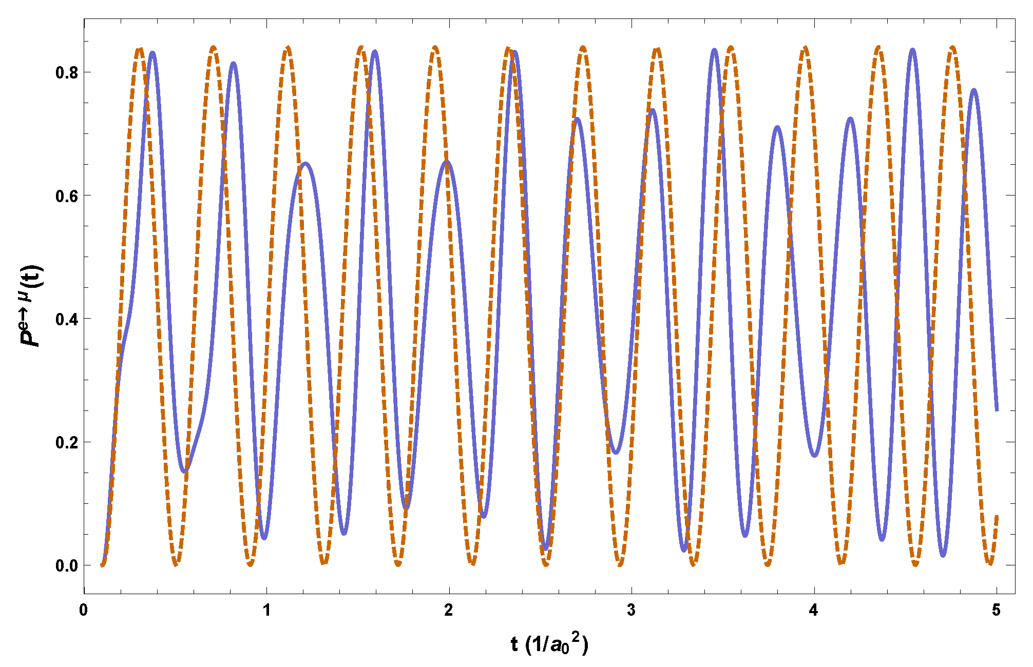
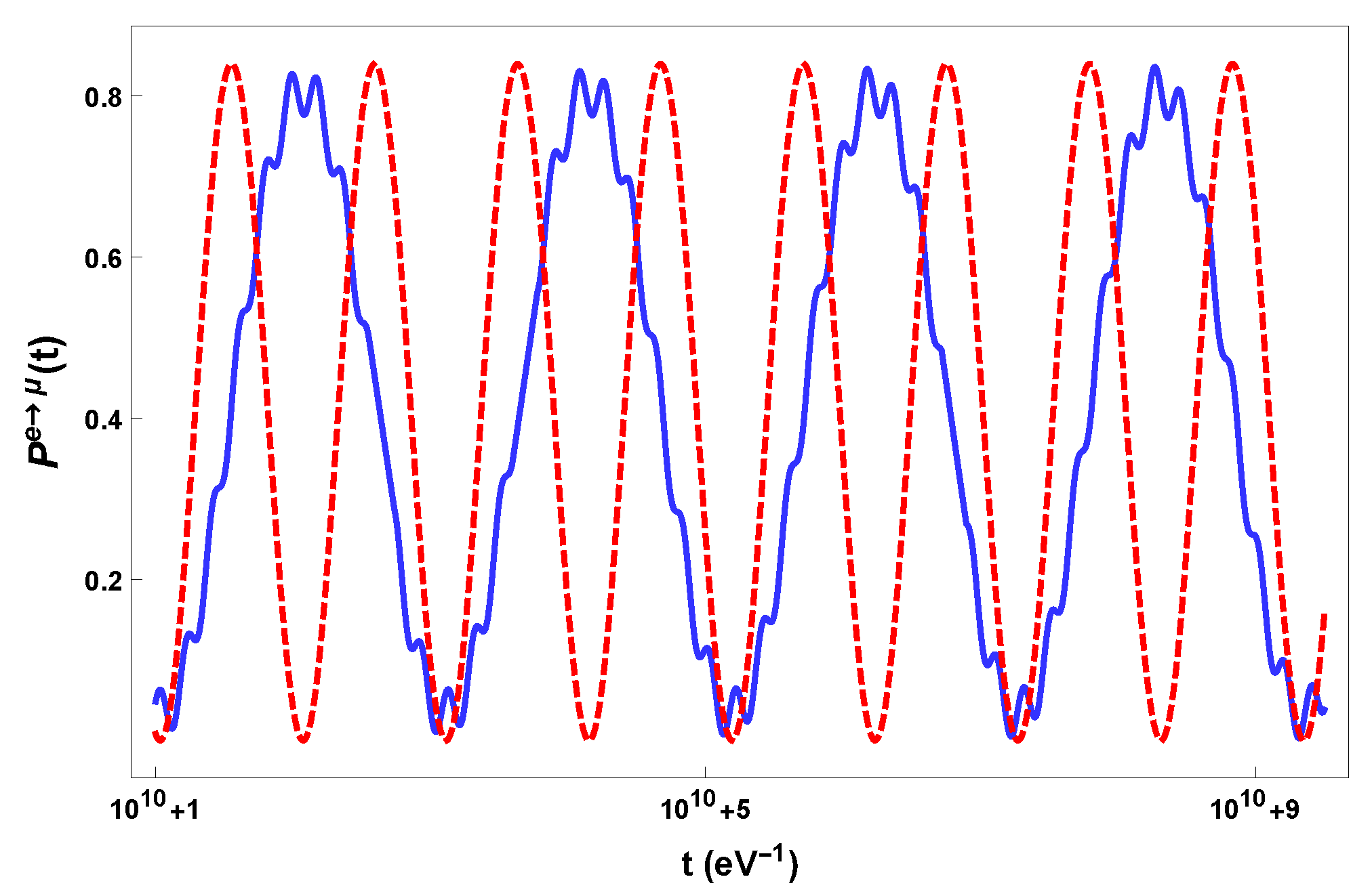
3.2. Flavor Oscillation Formulae

Now that we have an expansion of the flavor fields at our disposal, it is our task to devise a reasonable definition for the flavor oscillation formulae. The structure of the flavor representation is such that the standard quantum mechanical definition in terms of the inner product between states at different surfaces, e.g., $\langle {\nu }_e\left(\tau \right)|{\nu }_{\mu }\left({\tau }_0\right)\rangle$ or $\langle {\varphi }_A\left(\tau \right)|{\varphi }_B\left({\tau }_0\right)\rangle$, cannot work. Indeed, all such products vanish for $\tau \ne {\tau }_0$, given that they belong to mutually orthogonal Hilbert spaces as a consequence of unitarily inequivalence for distinct surfaces, in the infinite volume limit. We ought to seek a definition in terms of the matrix elements of suitable operators. The natural candidates, given the underlying $U\left(1\right)$ invariance, are the Noether charges of Equations (8) and (16). Let us tentatively define analogous “flavor” charges out of the operators of Equations (63) and (64):

$$\begin{array}{ccc}\hfill {\mathcal{Q}}_{F,\alpha }\left(\tau \right)& =& \sum _{k,s}\left(a_{k,s;\alpha }^{†}\left(\tau \right)a_{k,s\alpha }\left(\tau \right)-b_{k,s;\alpha }^{†}\left(\tau \right)b_{k,s;\alpha }\left(\tau \right)\right),\hfill \\ \hfill {\mathcal{Q}}_{B,\beta }\left(\tau \right)& =& \sum _k\left(c_{k;\beta }^{†}\left(\tau \right)c_{k;\beta }\left(\tau \right)-d_{k;\beta }^{†}\left(\tau \right)d_{k;\beta }\left(\tau \right)\right),\hfill \end{array}$$

(85)

where it is understood that $\alpha =e,\mu$ and $\beta =A,B$. These operators have several desirable properties:

• the one particle-states $|{\nu }_{k,s;\alpha }\left(\tau \right)\rangle$ and $|{\varphi }_{k;\beta }\left(\tau \right)\rangle$ are eigenstates, respectively, of ${\mathcal{Q}}_{F,\alpha }\left(\tau \right)$ and ${\mathcal{Q}}_{B,\beta }\left(\tau \right)$ with eigenvalue 1;
• states at different surface argument are $not$ generally eigenstates $\mathcal{Q}\left(\tau \right)|\nu \left({\tau }_0\right)\rangle \ne \lambda |\nu \left({\tau }_0\right)\rangle$. The expectation values $\langle {\nu }_{\alpha }\left({\tau }_0\right)|{\mathcal{Q}}_{\gamma }\left(\tau \right)|{\nu }_{\alpha }\left({\tau }_0\right)\rangle$ measure “how much” of flavor $\gamma$, as defined at surface $\tau$, is in the state of flavor $\alpha$, as defined at surface ${\tau }_0$.
• The sums over all the flavors of Equation (85) are constant, and equal the total Noether charges of Equation (8)

  $$\begin{array}{c}\hfill \sum _{\alpha =e,\mu }{\mathcal{Q}}_{F,\alpha }\left(\tau \right)=\sum _{j=1,2}{\mathcal{Q}}_{F,j}={\mathcal{Q}}_F;\sum _{\beta =A,B}{\mathcal{Q}}_{B,\beta }\left(\tau \right)=\sum _{j=1,2}{\mathcal{Q}}_{B,j}={\mathcal{Q}}_B.\end{array}$$

  (86)

It is clear that a sensible definition of the oscillation formulas is

$$P_{k,s}^{\alpha \to \gamma }(\tau ,{\tau }_0)=\langle {\nu }_{k,s;\alpha }\left({\tau }_0\right)|{\mathcal{Q}}_{F,\gamma }\left(\tau \right)|{\nu }_{k,s;\alpha }\left({\tau }_0\right)\rangle -\langle 0_f^F\left({\tau }_0\right)|{\mathcal{Q}}_{F,\gamma }\left(\tau \right)|0_f^F\left({\tau }_0\right)\rangle$$

(87)

with $\alpha ,\gamma =e,\mu$ for fermions and

$$P_k^{\beta \to \delta }(\tau ,{\tau }_0)=\langle {\varphi }_{k;\beta }\left({\tau }_0\right)|{\mathcal{Q}}_{B,\delta }\left(\tau \right)|{\varphi }_{k;\beta }\left({\tau }_0\right)\rangle -\langle 0_f^B\left({\tau }_0\right)|{\mathcal{Q}}_{B,\delta }\left(\tau \right)|0_f^B\left({\tau }_0\right)\rangle$$

(88)

with $\beta ,\delta =A,B$ for bosons. The last terms of Equations (87) and (88) are subtracted to achieve normal ordering with respect to the corresponding flavor vacuum. The quantities thus defined can be indeed interpreted as probabilities, since

$$\sum _{\gamma =e,\mu }{P}_{k,s}^{\alpha \to \gamma }(\tau ,{\tau }_0)=1=\sum _{\delta =A,B}{P}_k^{\beta \to \delta }(\tau ,{\tau }_0)$$

(89)

as a consequence of Equations (86). In due course, we will show that Equations (87) and (88) reduce to the standard quantum mechanical oscillation formulae in the appropriate limits, proving that they constitute a proper generalization of the latter. The oscillation formulae can be computed explicitly with the aid of Equations (63) and (64) and exploiting the canonical (anti-)commutation relations. The result is

$$P_{k,s}^{\alpha \to \gamma }(\tau ,{\tau }_0)=\frac{{sin}^{2}2\theta }{2}\left[1-\sum _{q,r}\mathrm{Re}\left({\mathsf{\Delta }}_{k,s;q,r}^{\ast }\left({\tau }_0\right){\mathsf{\Delta }}_{k,s;q,r}\left(\tau \right)+{\mathsf{\Omega }}_{k,s;q,r}^{\ast }\left({\tau }_0\right){\mathsf{\Omega }}_{k,s;q,r}\left(\tau \right)\right)\right]$$

(90)

for fermions, and

$$P_k^{\beta \to \delta }(\tau ,{\tau }_0)=\frac{{sin}^{2}2\theta }{2}\left[1-\sum _q\mathrm{Re}\left({\mathsf{\Delta }}_{k;q}^{\ast }\left({\tau }_0\right){\mathsf{\Delta }}_{k;q}\left(\tau \right)-{\mathsf{\Omega }}_{k;q}^{\ast }\left({\tau }_0\right){\mathsf{\Omega }}_{k;q}\left(\tau \right)\right)\right]$$

(91)

for bosons. As a direct consequence of Equations (66) and (67), it holds that

$$P_{k,s}^{\alpha \to \alpha }(\tau ,\tau )=1=P_k^{\beta \to \beta }(\tau ,\tau ),$$

(92)

as it should be for the survival probabilities at an initial time. Furthermore, given that there is no $CP$ violation by assumption (we are considering two flavor particle mixing), one also has $P_{k,s}^{\mu \to e}(\tau ,{\tau }_0)=P_{k,s}^{e\to \mu }(\tau ,{\tau }_0)$ and $P_k^{B\to A}(\tau ,{\tau }_0)=P_k^{A\to B}(\tau ,{\tau }_0)$. From the Equations (90) and (91), we can immediately extract the quantum mechanical limit. When all the field theoretic effects can be neglected, one has $\mathsf{\Omega }⟶0$ and $\left|\mathsf{\Delta }\right|⟶1$, for all the indices and for both fermions and bosons. The parenthetical terms of Equations (90) and (91) reduce to phase factors, in agreement with the results obtained in a quantum mechanics framework [23]. We can now ask whether the probabilities are left unchanged by variation of the mass and flavor representations. A glance at their definitions (87) and (88) reveals that they are not local observables: they generally involve operators and states defined on distinct surfaces $\tau$ and ${\tau }_0$. Therefore, we cannot expect them to be invariant on the grounds of local covariance. It is actually the case that for generic changes of mass representations, the probabilities are not left invariant. This is because the two representations may not agree on the quantum numbers, and thus on the interpretation, of the particle states. It is important to recognize that such a feature is not exclusively related to curved space: even in flat space we cannot expect to have the same form for the oscillation probabilities phrased in terms of, say, sharp momentum eigenstates and wavepackets. The probabilities themselves would indeed have a different physical meaning.

On the other hand, if the two representations agree on the meaning of the particle states (of course they need not agree on the particle content of the states, the number of particles or antiparticles they carry), i.e., assign the same set of quantum numbers, the resulting probabilities are identical. For any two such representations, the mass Bogoliubov coefficients shall be diagonal

$$\begin{array}{ccc}\hfill X_{k,s;q,r;j}& =& {\delta }_{k,q}{\delta }_{s,r}{X}_{k,s;j};Y_{k,s;q,r;j}={\delta }_{k,q}{\delta }_{s,r}{Y}_{k,s;j}\hfill \\ \hfill X_{k;q;j}& =& {\delta }_{k,q}{X}_{k;j};Y_{k;q;j}={\delta }_{k,q}{Y}_{k;j},\hfill \end{array}$$

so that the Equations (81)–(84) hold. Then, we have

$$\begin{array}{ccc}\hfill & & {\tilde{\mathsf{\Delta }}}_{k,s;q,r}^{\ast }\left({\tau }_0\right){\tilde{\mathsf{\Delta }}}_{k,s;q,r}\left(\tau \right)+{\tilde{\mathsf{\Omega }}}_{k,s;q,r}^{\ast }\left({\tau }_0\right){\tilde{\mathsf{\Omega }}}_{k,s;q,r}\left(\tau \right)=\hfill \\ \hfill & & \left({\mathsf{\Delta }}_{k,s;q,r}^{\ast }\left({\tau }_0\right){\mathsf{\Delta }}_{k,s;q,r}\left(\tau \right)+{\mathsf{\Omega }}_{k,s;q,r}^{\ast }\left({\tau }_0\right){\mathsf{\Omega }}_{k,s;q,r}\left(\tau \right)\right)\left(|X_{k,s;2}{|}^2|X_{q,r;1}{|}^2+ |X_{k,s;2}{|}^2{\left|Y_{q,r;1}\right|}^2\right) +\hfill \\ & & \left({\mathsf{\Delta }}_{k,s;q,r}\left({\tau }_0\right){\mathsf{\Delta }}_{k,s;q,r}^{\ast }\left(\tau \right)+{\mathsf{\Omega }}_{k,s;q,r}\left({\tau }_0\right){\mathsf{\Omega }}_{k,s;q,r}^{\ast }\left(\tau \right)\right)\left(|Y_{k,s;2}{|}^2|X_{q,r;1}{|}^2+ |Y_{k,s;2}{|}^2{\left|Y_{q,r;1}\right|}^2\right)\hfill \end{array}$$

(93)

for the fermionic coefficients and

$$\begin{array}{ccc}\hfill & & {\tilde{\mathsf{\Delta }}}_{k;q}^{\ast }\left({\tau }_0\right){\tilde{\mathsf{\Delta }}}_{k;q}\left(\tau \right)-{\tilde{\mathsf{\Omega }}}_{k;q}^{\ast }\left({\tau }_0\right){\tilde{\mathsf{\Omega }}}_{k;q}\left(\tau \right)=\hfill \\ \hfill & & \left({\mathsf{\Delta }}_{k;q}^{\ast }\left({\tau }_0\right){\mathsf{\Delta }}_{k;q}\left(\tau \right)-{\mathsf{\Omega }}_{k;q}^{\ast }\left({\tau }_0\right){\mathsf{\Omega }}_{k;q}\left(\tau \right)\right)\left(|X_{k;2}{|}^2|X_{q;1}{|}^2- |X_{k;2}{|}^2{\left|Y_{q;1}\right|}^2\right) +\hfill \\ & & \left({\mathsf{\Delta }}_{k;q}\left({\tau }_0\right){\mathsf{\Delta }}_{k;q}^{\ast }\left(\tau \right)-{\mathsf{\Omega }}_{k;q}\left({\tau }_0\right){\mathsf{\Omega }}_{k;q}^{\ast }\left(\tau \right)\right)\left(|Y_{k;2}{|}^2|Y_{q;1}{|}^2- |Y_{k;2}{|}^2{\left|X_{q;1}\right|}^2\right)\hfill \end{array}$$

(94)

for the bosonic coefficients. Considering that, by Equations (20) and (22), we have

$$\begin{array}{c}\hfill |X_{k,s;j}{|}^2+ |Y_{k,s;j}{|}^2=1= |X_{k;j}{|}^2-{\left|Y_{k;j}\right|}^2\end{array}$$

for each $j=1,2$, we conclude that

$$\begin{array}{ccc}\hfill & & \mathrm{Re}\left({\tilde{\mathsf{\Delta }}}_{k,s;q,r}^{\ast }\left({\tau }_0\right){\tilde{\mathsf{\Delta }}}_{k,s;q,r}\left(\tau \right)+{\tilde{\mathsf{\Omega }}}_{k,s;q,r}^{\ast }\left({\tau }_0\right){\tilde{\mathsf{\Omega }}}_{k,s;q,r}\left(\tau \right)\right)\hfill \\ & & =\mathrm{Re}\left({\mathsf{\Delta }}_{k,s;q,r}^{\ast }\left({\tau }_0\right){\mathsf{\Delta }}_{k,s;q,r}\left(\tau \right)+{\mathsf{\Omega }}_{k,s;q,r}^{\ast }\left({\tau }_0\right){\mathsf{\Omega }}_{k,s;q,r}\left(\tau \right)\right)\hfill \end{array}$$

(95)

and

$$\mathrm{Re}\left({\tilde{\mathsf{\Delta }}}_{k;q}^{\ast }\left({\tau }_0\right){\tilde{\mathsf{\Delta }}}_{k;q}\left(\tau \right)-{\tilde{\mathsf{\Omega }}}_{k;q}^{\ast }\left({\tau }_0\right){\tilde{\mathsf{\Omega }}}_{k;q}\left(\tau \right)\right)=\mathrm{Re}\left({\mathsf{\Delta }}_{k;q}^{\ast }\left({\tau }_0\right){\mathsf{\Delta }}_{k;q}\left(\tau \right)-{\mathsf{\Omega }}_{k;q}^{\ast }\left({\tau }_0\right){\mathsf{\Omega }}_{k;q}\left(\tau \right)\right).$$

(96)

This is sufficient to prove that the oscillation formulae of Equations (90) and (91) are identical in the tilded and untilded representations.

3.3. Neutrino Oscillations in Cosmological Metrics

We can now work out the transition probabilities for a given metric. We start with the fermionic probabilities in the class of conformally flat metrics of Equation (25). The first, trivial, example is the flat space metric with $\mathcal{A}\left(t\right)=1$. The solutions to the Dirac equations are the well-known plane waves. Without loss of generality, we can take the spin index to represent the eigenvalue of $S_z$, the third component, while the natural surfaces are those with $t=const.$. The mixing Bogoliubov coefficients are fully diagonal for momenta along the third axis ${\mathsf{\Delta }}_{\mathit{k},s;\mathit{q},r}\left(t\right)={\delta }^3(\mathit{k}-\mathit{q}){\delta }_{r,s}{\mathsf{\Delta }}_{\mathit{k}}^0\left(t\right);{\mathsf{\Omega }}_{\mathit{k},s;\mathit{q},r}\left(t\right)={\delta }^3(\mathit{k}-\mathit{q}){\delta }_{r,s}{(-1)}^{s-\frac{1}{2}}{\mathsf{\Omega }}_{\mathit{k}}^0\left(t\right)$, and the flat space coefficients satisfy ${\mathsf{\Delta }}_{\mathit{k}}^0\left(t\right)= |{\mathsf{\Delta }}_{\mathit{k}}^0|e^{i\left({\omega }_{\mathit{k};2}-{\omega }_{\mathit{k};1}\right)t};{\mathsf{\Omega }}_{\mathit{k}}^0\left(t\right)=\left|{\mathsf{\Omega }}_{\mathit{k}}^0\right|e^{i\left({\omega }_{\mathit{k};2}+{\omega }_{\mathit{k};1}\right)t}$, with ${\omega }_{\mathit{k};j}=\sqrt{{\mathit{k}}^2+m_j^2}$. The moduli are

$$\begin{array}{ccc}\hfill |{\mathsf{\Delta }}_{\mathit{k}}^0|& =& \sqrt{\frac{\left({\omega }_{\mathit{k};1}+m_1\right)\left({\omega }_{\mathit{k};2}+m_2\right)}{4{\omega }_{\mathit{k};1}{\omega }_{\mathit{k};2}}}\left(1+\frac{{\mathit{k}}^2}{\left({\omega }_{\mathit{k};1}+m_1\right)\left({\omega }_{\mathit{k};2}+m_2\right)}\right)\hfill \\ \hfill |{\mathsf{\Omega }}_{\mathit{k}}^0|& =& \sqrt{\frac{\left({\omega }_{\mathit{k};1}+m_1\right)\left({\omega }_{\mathit{k};2}+m_2\right)}{4{\omega }_{\mathit{k};1}{\omega }_{\mathit{k};2}}}\left(\frac{\left|\mathit{k}\right|}{\left({\omega }_{\mathit{k};2}+m_2\right)}-\frac{\left|\mathit{k}\right|}{\left({\omega }_{\mathit{k};1}+m_1\right)}\right).\hfill \end{array}$$

(97)

Inserting these expressions in the general formula Equation (90), we find

$$P_{\mathit{k},s}^{e\to \mu }(t,0)={sin}^{2}2\theta \left[|{\mathsf{\Delta }}_{\mathit{k}}^0{|}^2{sin}^2\left(\frac{\left({\omega }_{\mathit{k};2}-{\omega }_{\mathit{k};1}\right)t}{2}\right)+{\left|{\mathsf{\Omega }}_{\mathit{k}}^0\right|}^2{sin}^2\left(\frac{\left({\omega }_{\mathit{k};2}+{\omega }_{\mathit{k};1}\right)t}{2}\right)\right],$$

(98)

which coincides with the flat space result [14] and with the Pontecorvo probability in the ultrarelativistic limit $|{\mathsf{\Omega }}_{\mathit{k}}^0|\to 0$ and $|{\mathsf{\Delta }}_{\mathit{k}}^0|\to 1$. Before moving on to less trivial examples, let us work out the flat space probabilities in a different mass representation, given by the common eigenstates of energy and total angular momentum, namely

$$\begin{array}{ccc}\hfill {\mathcal{U}}_{\omega ,{\kappa }_J,{\mu }_J;j}(t,r,\theta ,\varphi )& =& e^{-i\omega t}\sqrt{\frac{\omega +m_j}{2\omega r^2}}\left(\begin{array}{c}{P}_{{\kappa }_J}\left({\lambda }_{j}r\right)H_{{\kappa }_J,{\mu }_J}(\theta ,\varphi )\\ \sqrt{\frac{\omega -m_j}{\omega +m_j}}{P}_{{\kappa }_J}\left({\lambda }_{j}r\right)H_{-{\kappa }_J,{\mu }_J}(\theta ,\varphi )\end{array}\right)\hfill \\ \hfill {\mathcal{V}}_{\omega ,{\kappa }_J,{\mu }_J;j}(t,r,\theta ,\varphi )& =& e^{i\omega t}\sqrt{\frac{\omega +m_j}{2\omega r^2}}\left(\begin{array}{c}-\sqrt{\frac{\omega -m_j}{\omega +m_j}}{P}_{{\kappa }_J}\left(-{\lambda }_{j}r\right)H_{{\kappa }_J,{\mu }_J}(\theta ,\varphi )\\ P_{{\kappa }_J}\left(-{\lambda }_{j}r\right)H_{-{\kappa }_J,{\mu }_J}(\theta ,\varphi )\end{array}\right).\hfill \end{array}$$

(99)

They solve the flat space Dirac equation in spherical coordinates with energy $\omega$, third component of the total angular momentum ${\mu }_J$ and generalized spin-orbit quantum number ${\kappa }_J$. The orbital quantum number is denoted ${\mu }_J$ in order to avoid confusion with the masses $m_j$: J is the total angular momentum, while j is the mass field label. The functions $H_{\kappa ,\mu }$ are the two component spherical spinors [80], while the radial functions have the form $P_{{\kappa }_j}\left({\lambda }_{j}r\right)=r{j}_{{\kappa }_j}\left({\lambda }_{j}r\right)$ with $j_n\left(r\right)$ the spherical Bessel functions of order n [78] and ${\lambda }_j=\sqrt{{\omega }^2-m_j^2}$ the radial momentum. Of course, one has the intrinsic constraint on the energy $\omega \ge m_j$. The computation of the Bogoliubov coefficients is straightforward, and only requires the completeness relation of the spherical Bessel functions. The result is

$$\begin{array}{ccc}\hfill {\mathsf{\Delta }}_{{\omega }^{\prime },{\kappa }_J^{\prime },{\mu }_J^{\prime };\omega ,{\kappa }_J,{\mu }_J}\left(t\right)& =& {\delta }_{{\omega }^{\prime },\sqrt{{\omega }^2+\mathsf{\Delta }{m}^2}}{\delta }_{{\kappa }_J^{\prime },{\kappa }_J}{\delta }_{{\mu }_J^{\prime },{\mu }_J}\left|{\mathsf{\Delta }}_{\omega ,{\omega }^{\prime }}^0\right|e^{i\left({\omega }^{\prime }-\omega \right)t}\hfill \\ \hfill {\mathsf{\Omega }}_{{\omega }^{\prime },{\kappa }_J^{\prime },{\mu }_J^{\prime };\omega ,{\kappa }_J,{\mu }_J}\left(t\right)& =& {\delta }_{{\omega }^{\prime },\sqrt{{\omega }^2+\mathsf{\Delta }{m}^2}}{\delta }_{{\kappa }_J^{\prime },{\kappa }_J}{\delta }_{{\mu }_J^{\prime },{\mu }_J}\left|{\mathsf{\Omega }}_{\omega ,{\omega }^{\prime }}^0\right|e^{i\left({\omega }^{\prime }+\omega \right)t}.\hfill \end{array}$$

(100)

Here, $\mathsf{\Delta }{m}^2=m_2^2-m_1^2$ and

$$\begin{array}{ccc}\hfill |{\mathsf{\Delta }}_{\omega ,{\omega }^{\prime }}^0|& =& \sqrt{\frac{\left({\omega }^{\prime }+m_2\right)\left(\omega +m_1\right)}{4{\omega }^{\prime }\omega }}\left(1+\sqrt{\frac{\left({\omega }^{\prime }-m_2\right)\left(\omega -m_1\right)}{\left(\omega +m_1\right)\left({\omega }^{\prime }+m_2\right)}}\right)\hfill \\ \hfill |{\mathsf{\Omega }}_{\omega ,{\omega }^{\prime }}^0|& =& \sqrt{\frac{\left({\omega }^{\prime }+m_2\right)\left(\omega +m_1\right)}{4{\omega }^{\prime }\omega }}\left(\sqrt{\frac{{\omega }^{\prime }-m_2}{{\omega }^{\prime }+m_2}}-\sqrt{\frac{\omega -m_1}{\omega +m_1}}\right).\hfill \end{array}$$

(101)

It is immediately seen that the coefficients of Equation (101) are numerically the same as the coefficient of Equation (97) when ${\omega }^{{}^{\prime }2}-m_2^2={\omega }^2-m_1^2={\mathit{k}}^2$, which is exactly the condition imposed by the delta functions in Equation (100) for some given ${\mathit{k}}^2$. The interesting feature of the coefficients of Equation (100) is that they are not diagonal: they connect states of mass 1 with energy ${\omega }_{\mathit{k};1}$ with the states of mass 2 with energy ${\omega }_{\mathit{k};2}=\sqrt{{\omega }_{\mathit{k};1}^2+\mathsf{\Delta }{m}^2}$, just as we would expect. Yet, they are “pseudo”-diagonal, in the sense that they only connect mass 2 modes with one specific mass 1 mode, and vice-versa. This is the reason why the resulting probabilities are exactly the same as Equation (98), except for a relabeling $\mathit{k}\to \omega$, with $\omega =\sqrt{{\mathit{k}}^2+m_1^2}$ referred to mass 1, and ${\omega }_{\mathit{k};2}\to \sqrt{{\omega }^2+\mathsf{\Delta }{m}^2}$. In flat space, the shift from momentum to energy eigenstates only leads to a fancier way to write down the same probabilities. Nonetheless, the expansion in terms of the angular momentum eigenstates of Equation (99) is very useful when Cartesian three-momentum is not a natural quantum number and spherical coordinates represent the natural choice for the description of the metric. We will meet such a case explicitly for the Schwarzschild black hole spacetime.

Let us now consider $\mathcal{A}\left(t\right)=e^{H_{0}t}$. We have derived the Dirac modes in the previous sections, so that we only need to compute the Bogoliubov coefficients and plug them in the general Equation (90). We use the boundary condition of Equation (43) and compute the inner products on constant t (or equivalently constant $\tau$) surfaces. The result is

$$\begin{array}{ccc}\hfill {\mathsf{\Delta }}_{\mathit{k},s;\mathit{q},r}\left(t\right)& =& {\delta }_{s,r}{\delta }^3(\mathit{k}-\mathit{q})\frac{\pi ku}{2\sqrt{cos\left(\frac{i\pi m_2}{H}\right)cos\left(\frac{i\pi m_1}{H}\right)}}\left(J_{{\nu }_2}^{\ast }\left(ku\right)J_{{\nu }_1}\left(ku\right)+J_{{\nu }_2-1}^{\ast }\left(ku\right)J_{{\nu }_1-1}\left(ku\right)\right)\hfill \end{array}$$

(102)

$$\begin{array}{ccc}\hfill {\mathsf{\Omega }}_{\mathit{k},s;\mathit{q},r}\left(t\right)& =& {\delta }_{s,r}{(-1)}^{s-\frac{1}{2}}{\delta }^3(\mathit{k}-\mathit{q})\frac{\pi ku}{2\sqrt{cos\left(\frac{i\pi m_2}{H}\right)cos\left(\frac{i\pi m_1}{H}\right)}}\left(J_{{\nu }_1}^{\ast }\left(ku\right)J_{-{\nu }_2}\left(ku\right)-J_{{\nu }_1-1}^{\ast }\left(ku\right)J_{1-{\nu }_2}\left(ku\right)\right)\hfill \end{array}$$

(103)

where $u=-\tau =\frac{e^{-H_{0}t}}{H_0}$. Inserting these expressions in Equation (90), we obtain

$$\begin{array}{ccc}\hfill & & P_{k,s}^{e\to \mu }(t,t_0)=\frac{{sin}^{2}2\theta }{2}\{1-\frac{{\pi }^2{k}^2{u}_{0}u}{4cos\left(\frac{i\pi m_2}{H}\right)cos\left(\frac{i\pi m_1}{H}\right)}\hfill \\ \hfill & & \times \mathrm{Re}[\left[J_{{\nu }_2}\left(k{u}_0\right)J_{{\nu }_1}^{\ast }\left(k{u}_0\right)+J_{{\nu }_2-1}\left(k{u}_0\right)J_{{\nu }_1-1}^{\ast }\left(k{u}_0\right)\right]\left[J_{{\nu }_2}^{\ast }\left(ku\right)J_{{\nu }_1}\left(ku\right)+J_{{\nu }_2-1}^{\ast }\left(ku\right)J_{{\nu }_1-1}\left(ku\right)\right]\hfill \\ & & +\left[J_{{\nu }_1}\left(k{u}_0\right)J_{-{\nu }_2}^{\ast }\left(k{u}_0\right)-J_{{\nu }_1-1}\left(k{u}_0\right)J_{1-{\nu }_2}^{\ast }\left(k{u}_0\right)\right]\left[J_{{\nu }_1}^{\ast }\left(ku\right)J_{-{\nu }_2}\left(ku\right)-J_{{\nu }_1-1}^{\ast }\left(ku\right)J_{1-{\nu }_2}\left(ku\right)\right]\left]\right\}.\hfill \end{array}$$

(104)

where, as before, $u=\frac{e^{-H_{0}t}}{H_0}$ and $u_0=\frac{e^{-H_0{t}_0}}{H_0}$. Although the expression may look quite complicated, it really amounts to an amplitude varying oscillatory behaviour. This can be neatly seen from Figure 1 where Equation (104) is plotted for sample values of masses and momenta.

For the radiation dominated spacetime $\mathcal{A}\left(t\right)=a_0{t}^{\frac{1}{2}}$, we have the Bogoliubov coefficients

$$\begin{array}{ccc}& & {\mathsf{\Delta }}_{\mathit{k},s;\mathit{q},r}\left(t\right)={\delta }_{s,r}{\delta }^3(\mathit{k}-\mathit{q})\frac{1}{\sqrt[4]{4m_1{m}_2{t}^2}}{e}^{-\frac{\pi k^2(m_1+m_2)}{4m_1{m}_2{a}_0^2}}\{W_{{\kappa }_2,\frac{1}{4}}^{\ast }(-2i{m}_{2}t)W_{{\kappa }_1,\frac{1}{4}}(-2i{m}_{1}t)\hfill \\ \hfill & & +\frac{4k^2}{m_1{m}_2{a}_0^{2}t}\left[\frac{1}{4}{W}_{{\kappa }_2,\frac{1}{4}}^{\ast }(-2i{m}_{2}t)-\frac{1}{8}\left(1+\frac{i{k}^2}{m_2{a}_0^2}\right)W_{{\kappa }_2-1,\frac{1}{4}}^{\ast }(-2i{m}_{2}t)\right]\left[\frac{1}{4}{W}_{{\kappa }_1,\frac{1}{4}}(-2i{m}_{1}t)-\frac{1}{8}\left(1-\frac{i{k}^2}{m_1{a}_0^2}\right)W_{{\kappa }_1-1,\frac{1}{4}}(-2i{m}_{1}t)\right]\}\hfill \end{array}$$

(105)

$$\begin{array}{ccc}& & {\mathsf{\Omega }}_{\mathit{k},s;\mathit{q},r}\left(t\right)={\delta }_{s,r}{(-1)}^{s-\frac{1}{2}}{\delta }^3(\mathit{k}-\mathit{q})\frac{k}{\sqrt[4]{2m_1{\left(2m_2\right)}^3{a}_0^4{t}^2}}{e}^{-\frac{\pi k^2(m_1+m_2)}{4m_1{m}_2{a}_0^2}}\{W_{{\kappa }_1,\frac{1}{4}}^{\ast }(-2i{m}_{1}t)W_{-{\kappa }_2,\frac{1}{4}}\left(2i{m}_{2}t\right)\hfill \\ \hfill & & +\frac{k^2}{m_1{m}_2{a}_0^{2}t}\left[\frac{1}{4}{W}_{{\kappa }_1,\frac{1}{4}}^{\ast }(-2i{m}_{1}t)-\frac{1}{8}\left(1+\frac{i{k}^2}{m_1{a}_0^2}\right)W_{{\kappa }_1-1,\frac{1}{4}}^{\ast }(-2i{m}_{1}t)\right]\left[W_{-{\kappa }_2,\frac{1}{4}}\left(2i{m}_{2}t\right)+\frac{2i{m}_2{a}_0^2}{k^2}{W}_{-{\kappa }_2+1,\frac{1}{4}}\left(2i{m}_{2}t\right)\right]\}\hfill \end{array}$$

(106)

where $W_{\kappa ,\mu }\left(z\right)$ are the Whittaker functions [78] and ${\kappa }_j=\frac{1}{4}\left(1+\frac{2i{k}^2}{a_0^2{m}_j}\right)$ for $j=1,2$. The resulting transition probabilities are

$$\begin{array}{ccc}\hfill & & P_{k,s}^{e\to \mu }(t,t_0)=\frac{{sin}^{2}2\theta }{2}\{1-\mathrm{Re}[\frac{1}{\sqrt{4m_1{m}_2{t}_{0}t}}{e}^{-\frac{\pi k^2(m_1+m_2)}{2m_1{m}_2{a}_0^2}}\{W_{{\kappa }_2,\frac{1}{4}}(-2i{m}_2{t}_0)W_{{\kappa }_1,\frac{1}{4}}^{\ast }(-2i{m}_1{t}_0)\hfill \\ \hfill & & +\frac{4k^2}{m_1{m}_2{a}_0^2{t}_0}\left(\frac{1}{4}{W}_{{\kappa }_2,\frac{1}{4}}(-2i{m}_2{t}_0)-\frac{1}{8}\left(1-\frac{i{k}^2}{m_2{a}_0^2}\right)W_{{\kappa }_2-1,\frac{1}{4}}(-2i{m}_2{t}_0)\right)\left(\frac{1}{4}{W}_{{\kappa }_1,\frac{1}{4}}^{\ast }(-2i{m}_1{t}_0)-\frac{1}{8}\left(1+\frac{i{k}^2}{m_1{a}_0^2}\right)W_{{\kappa }_1-1,\frac{1}{4}}^{\ast }(-2i{m}_1{t}_0)\right)\}\hfill \\ \hfill & & \times \{W_{{\kappa }_2,\frac{1}{4}}^{\ast }(-2i{m}_{2}t)W_{{\kappa }_1,\frac{1}{4}}(-2i{m}_{1}t)\hfill \\ \hfill & & +\frac{4k^2}{m_1{m}_2{a}_0^{2}t}\left(\frac{1}{4}{W}_{{\kappa }_2,\frac{1}{4}}^{\ast }(-2i{m}_{2}t)-\frac{1}{8}\left(1+\frac{i{k}^2}{m_2{a}_0^2}\right)W_{{\kappa }_2-1,\frac{1}{4}}^{\ast }(-2i{m}_{2}t)\right)\left(\frac{1}{4}{W}_{{\kappa }_1,\frac{1}{4}}(-2i{m}_{1}t)-\frac{1}{8}\left(1-\frac{i{k}^2}{m_1{a}_0^2}\right)W_{{\kappa }_1-1,\frac{1}{4}}(-2i{m}_{1}t)\right)\}\hfill \\ \hfill & & +\frac{k^2}{\sqrt{2m_1{\left(2m_2\right)}^3{a}_0^4{t}_{0}t}}{e}^{-\frac{\pi k^2(m_1+m_2)}{2m_1{m}_2{a}_0^2}}\{W_{{\kappa }_1,\frac{1}{4}}(-2i{m}_1{t}_0)W_{-{\kappa }_2,\frac{1}{4}}^{\ast }\left(2i{m}_2{t}_0\right)\hfill \\ \hfill & & +\frac{k^2}{m_1{m}_2{a}_0^2{t}_0}\left(\frac{1}{4}{W}_{{\kappa }_1,\frac{1}{4}}(-2i{m}_1{t}_0)-\frac{1}{8}\left(1-\frac{i{k}^2}{m_1{a}_0^2}\right)W_{{\kappa }_1-1,\frac{1}{4}}(-2i{m}_1{t}_0)\right)\left(W_{-{\kappa }_2,\frac{1}{4}}^{\ast }\left(2i{m}_2{t}_0\right)-\frac{2i{m}_2{a}_0^2}{k^2}{W}_{-{\kappa }_2+1,\frac{1}{4}}^{\ast }\left(2i{m}_2{t}_0\right)\right)\}\hfill \\ \hfill & & \times \{W_{{\kappa }_1,\frac{1}{4}}^{\ast }(-2i{m}_{1}t)W_{-{\kappa }_2,\frac{1}{4}}\left(2i{m}_{2}t\right)\hfill \\ & & +\frac{k^2}{m_1{m}_2{a}_0^{2}t}\left(\frac{1}{4}{W}_{{\kappa }_1,\frac{1}{4}}^{\ast }(-2i{m}_{1}t)-\frac{1}{8}\left(1+\frac{i{k}^2}{m_1{a}_0^2}\right)W_{{\kappa }_1-1,\frac{1}{4}}^{\ast }(-2i{m}_{1}t)\right)\left(W_{-{\kappa }_2,\frac{1}{4}}\left(2i{m}_{2}t\right)+\frac{2i{m}_2{a}_0^2}{k^2}{W}_{-{\kappa }_2+1,\frac{1}{4}}\left(2i{m}_{2}t\right)\right)\left\}\right]\}.\hfill \end{array}$$

(107)

The equation above is quite involved, but shares the same features of the oscillation formulae (104): both amplitude and phase vary with time, and can differ significantly from their flat space counterpart. In Figure 2, we compare Equation (107) with the Pontecorvo formula in flat space for some sample values of the parameters.

3.4. Neutrino Oscillations in Asymptotically Flat Manifolds

One remarkable aspect of the spatially flat FRW metrics is that we were able to derive exact analytical expressions for the transition probabilities (i.e., Equations (104) and (107)), due to the knowledge of the analytic form of the modes (Section 2). In most of the metrics, however, analytical solutions are not available, and we have to resort to some kind of approximation. Approximate oscillation formulae can be derived in a simple fashion for spacetimes that admit asymptotically flat regions. To show that, suppose that the underlying spacetime has two asymptotically flat regions at past and future infinities $T_{IN}={\bigcup }_{\tau \le {\tau }_I}{\mathsf{\Sigma }}_{\tau }$ and $T_{OUT}={\bigcup }_{\tau \ge {\tau }_O}{\mathsf{\Sigma }}_{\tau }$, with ${\tau }_O>{\tau }_I$. This is quite a weak requirement and is satisfied by several metrics, as is the case, for instance, of the Schwarzschild spacetime. On $T_{IN}$ and $T_{OUT}$, the metric is approximately flat, so that approximate solutions to the Dirac equations are the flat space spinors. Denote the sets of solutions which are positive (negative) energy in the two regions by $\left\{{\mathcal{U}}_{k,s;j}^{IN}\left(x\right),{\mathcal{V}}_{k,s;j}^{IN}\left(x\right)\right\}$ and $\left\{{\mathcal{U}}_{k,s;j}^{OUT}\left(x\right),{\mathcal{V}}_{k,s;j}^{OUT}\left(x\right)\right\}$, respectively. Because both are complete, the fields can be expanded in either the $IN$ or $OUT$ modes, and the two sets are related by the Bogoliubov transformation

$$\begin{array}{ccc}\hfill {\mathcal{U}}_{k^{\prime },s^{\prime };j}^{OUT}& =& \sum _{k,s}\left(X_{k^{\prime },s^{\prime };k,s;j}^{\ast }{\mathcal{U}}_{k,s;j}^{IN}+Y_{k^{\prime },s^{\prime };k,s;j}^{\ast }{\mathcal{V}}_{k,s;j}^{IN}\right)\hfill \\ \hfill {\mathcal{V}}_{k^{\prime },s^{\prime };j}^{OUT}& =& \sum _{k,s}\left(X_{k^{\prime },s^{\prime };k,s;j}{\mathcal{V}}_{k,s;j}^{IN}-Y_{k^{\prime },s^{\prime };k,s;j}{\mathcal{U}}_{k,s;j}^{IN}\right).\hfill \end{array}$$

(108)

Here, the (mass) Bogoliubov coefficients are just the same as in Section 2, given by the inner products of $OUT$ and $IN$ modes, except that they now connect two special mass representations: the (locally) flat space representations of $T_{IN}$ and $T_{OUT}$. Now, suppose we want to determine the transition probabilities for neutrinos traveling all the way from the infinite past $T_{IN}$ to the infinite future $T_{OUT}$. Then, we select $\tau >{\tau }_O$ and ${\tau }_0<{\tau }_I$ and compute

$$\begin{array}{c}\hfill P_{k,s}^{e\to \mu }(\tau ,{\tau }_0)=\frac{{sin}^{2}2\theta }{2}\left[1-\sum _{q,r}\mathrm{Re}\left({\mathsf{\Delta }}_{k,s;q,r}^{OUT\ast }\left({\tau }_0\right){\mathsf{\Delta }}_{k,s;q,r}^{OUT}\left(\tau \right)+{\mathsf{\Omega }}_{k,s;q,r}^{OUT\ast }\left({\tau }_0\right){\mathsf{\Omega }}_{k,s;q,r}^{OUT}\left(\tau \right)\right)\right]\end{array}$$

(109)

where we have picked the flavor representation induced by the $OUT$ modes for definiteness (of course we could have picked the $IN$ representation as well). The mixing Bogoliubov coefficients ${\mathsf{\Delta }}^{OUT},{\mathsf{\Omega }}^{OUT}$ are trivial at $\tau$, where they match the flat space coefficients. The same is not true for these coefficients evaluated at ${\tau }_0$, in the $IN$ region. However, now Equations (77) and (78) come into play, giving the $OUT$ coefficients in terms of the $IN$ coefficients:

$$\begin{array}{ccc}\hfill {\mathsf{\Delta }}_{k,s;q,r}^{OUT}\left(\tau \right)& =& \sum _{k^{\prime },s^{\prime },q^{\prime },r^{\prime }}\{X_{k,s;k^{\prime },s^{\prime };2}{X}_{q,r;q^{\prime },r^{\prime };1}^{\ast }{\mathsf{\Delta }}_{k^{\prime },s^{\prime };q^{\prime },r^{\prime }}^{IN}\left(\tau \right)-X_{k,s;k^{\prime },s^{\prime };2}{Y}_{q,r;q^{\prime },r^{\prime };1}^{\ast }{\mathsf{\Omega }}_{k^{\prime },s^{\prime };q^{\prime },r^{\prime }}^{IN}\left(\tau \right)\hfill \\ & +& Y_{k,s;k^{\prime },s^{\prime };2}{X}_{q,r;q^{\prime },r^{\prime };1}^{\ast }{\mathsf{\Omega }}_{k^{\prime },s^{\prime };q^{\prime },r^{\prime }}^{IN\ast }\left(\tau \right)+Y_{k,s;k^{\prime },s^{\prime };2}{Y}_{q,r;q^{\prime },r^{\prime };1}^{\ast }{\mathsf{\Delta }}_{k^{\prime },s^{\prime };q^{\prime },r^{\prime }}^{IN\ast }\left(\tau \right)\},\hfill \end{array}$$

(110)

$$\begin{array}{ccc}\hfill {\mathsf{\Omega }}_{k,s;q,r}^{OUT}\left(\tau \right)& =& \sum _{k^{\prime },s^{\prime },q^{\prime },r^{\prime }}\{X_{k,s;k^{\prime },s^{\prime };2}{X}_{q,r;q^{\prime },r^{\prime };1}{\mathsf{\Omega }}_{k^{\prime },s^{\prime };q^{\prime },r^{\prime }}^{IN}\left(\tau \right)+X_{k,s;k^{\prime },s^{\prime };2}{Y}_{q,r;q^{\prime },r^{\prime };1}{\mathsf{\Delta }}_{k^{\prime },s^{\prime };q^{\prime },r^{\prime }}^{IN}\left(\tau \right)\hfill \\ & -& Y_{k,s;k^{\prime },s^{\prime };2}{X}_{q,r;q^{\prime },r^{\prime };1}{\mathsf{\Delta }}_{k^{\prime },s^{\prime };q^{\prime },r^{\prime }}^{IN\ast }\left(\tau \right)+Y_{k,s;k^{\prime },s^{\prime };2}{Y}_{q,r;q^{\prime },r^{\prime };1}{\mathsf{\Omega }}_{k^{\prime },s^{\prime };q^{\prime },r^{\prime }}^{IN\ast }\left(\tau \right)\}.\hfill \end{array}$$

(111)

Now, the $IN$ coefficients are trivial at ${\tau }_0$, so that we can use Equations (110) and (111) to easily obtain the $OUT$ coefficients at ${\tau }_0$.

In order to see this trick at work, consider the static Schwarzschild metric

$$d{s}^2=\left(1-\frac{2GM}{r}\right)d{t}^2-{\left(1-\frac{2GM}{r}\right)}^{-1}d{r}^2-r^{2}d{\mathsf{\Omega }}_{\left(2\right)}.$$

(112)

Here, $d{\mathsf{\Omega }}_{\left(2\right)}=d{\mathsf{\Theta }}^2+{sin}^2\mathsf{\Theta }d{\varphi }^2$ is the line element on the sphere. Let ${\left\{{\mathsf{\Sigma }}_n^{OUT}\right\}}_{n\in \mathbb{N}}$ and ${\left\{{\mathsf{\Sigma }}_m^{IN}\right\}}_{n\in \mathbb{N}}$ be two sequences of Cauchy surfaces, with each ${\mathsf{\Sigma }}_n^{OUT}$ lying in the causal past of the future null infinity $J^{-}\left({\mathcal{I}}^{+}\right)$ and each ${\mathsf{\Sigma }}_m^{IN}$ in the causal future of the past null infinity $J^{+}\left({\mathcal{I}}^{-}\right)$. In simple terms, any causal (timelike or lightlike) curve extending from the past ${\mathcal{I}}^{-}$ infinity to the future infinity ${\mathcal{I}}^{+}$ has to meet each of the ${\mathsf{\Sigma }}_n^{OUT}$ and ${\mathsf{\Sigma }}_n^{IN}$ at exactly one point, due to their characterization as Cauchy surfaces. We assume that as $n\to \infty$ the surfaces approach, respectively, ${\mathcal{I}}^{+}$ and ${\mathcal{I}}^{-}$. The index n is just a bookkeping variable to formalize such a limiting procedure: the choice of discrete indices is by no means compulsory, and we could as well use continuous indices to label the sequences. For large n, the surfaces ${\mathsf{\Sigma }}_n^{OUT}$ and ${\mathsf{\Sigma }}_n^{IN}$ span approximately flat regions of the Schwarzschild spacetime, where the Dirac equation is approximately solved by the flat space solutions of Equation (99). It follows that the mixing Bogoliubov coefficients, as defined with respect to the $IN$ modes, take the form of Equation (100)

$$\begin{array}{ccc}\hfill {\mathsf{\Delta }}_{{\omega }^{\prime },{\kappa }_J^{\prime },{\mu }_J^{\prime };\omega ,{\kappa }_J,{\mu }_J}^{IN}\left({\mathsf{\Sigma }}_n^{IN}\right)& =& {\delta }_{{\omega }^{\prime },\sqrt{{\omega }^2+\mathsf{\Delta }{m}^2}}{\delta }_{{\kappa }_J^{\prime },{\kappa }_J}{\delta }_{{\mu }_J^{\prime },{\mu }_J}\left|{\mathsf{\Delta }}_{\omega ,{\omega }^{\prime }}^0\right|e^{i{\varphi }^{-}(\omega ,n)}\hfill \\ \hfill {\mathsf{\Omega }}_{{\omega }^{\prime },{\kappa }_J^{\prime },{\mu }_J^{\prime };\omega ,{\kappa }_J,{\mu }_J}^{IN}\left({\mathsf{\Sigma }}_n^{IN}\right)& =& {\delta }_{{\omega }^{\prime },\sqrt{{\omega }^2+\mathsf{\Delta }{m}^2}}{\delta }_{{\kappa }_J^{\prime },{\kappa }_J}{\delta }_{{\mu }_J^{\prime },{\mu }_J}\left|{\mathsf{\Omega }}_{\omega ,{\omega }^{\prime }}^0\right|e^{i{\rho }^{-}(\omega ,n)},\hfill \end{array}$$

(113)

where ${\varphi }^{-}(\omega ,n),{\rho }^{-}(\omega ,n)$ are phase factors depending on $\omega$ and n. Similar expressions hold for the $OUT$ Bogoliubov coefficients on the $OUT$ surfaces:

$$\begin{array}{ccc}\hfill {\mathsf{\Delta }}_{{\omega }^{\prime },{\kappa }_J^{\prime },{\mu }_J^{\prime };\omega ,{\kappa }_J,{\mu }_J}^{OUT}\left({\mathsf{\Sigma }}_n^{OUT}\right)& =& {\delta }_{{\omega }^{\prime },\sqrt{{\omega }^2+\mathsf{\Delta }{m}^2}}{\delta }_{{\kappa }_J^{\prime },{\kappa }_J}{\delta }_{{\mu }_J^{\prime },{\mu }_J}\left|{\mathsf{\Delta }}_{\omega ,{\omega }^{\prime }}^0\right|e^{i{\varphi }^{+}(\omega ,n)}\hfill \\ \hfill {\mathsf{\Omega }}_{{\omega }^{\prime },{\kappa }_J^{\prime },{\mu }_J^{\prime };\omega ,{\kappa }_J,{\mu }_J}^{OUT}\left({\mathsf{\Sigma }}_n^{OUT}\right)& =& {\delta }_{{\omega }^{\prime },\sqrt{{\omega }^2+\mathsf{\Delta }{m}^2}}{\delta }_{{\kappa }_J^{\prime },{\kappa }_J}{\delta }_{{\mu }_J^{\prime },{\mu }_J}\left|{\mathsf{\Omega }}_{\omega ,{\omega }^{\prime }}^0\right|e^{i{\rho }^{+}(\omega ,n)}.\hfill \end{array}$$

(114)

We need now only to relate the $IN$ and $OUT$ mode via an equation of the form (108). The misalignment between the $IN$ and $OUT$ modes is here due to the Schwarzschild black hole, and the Bogoliubov coefficients that relate the two expansions are those characterizing the Hawking radiation of spin $1/2$ particles. The radiation is thermal and determined by the Hawking temperature $T_H=\frac{1}{8\pi GM}$, as derived in [58]. Therefore

$$\begin{array}{ccc}\hfill X_{{\omega }^{\prime },{\kappa }_J^{\prime },{\mu }_J^{\prime };\omega ,{\kappa }_J,{\mu }_J;j}& =& {\delta }_{\omega ,{\omega }^{\prime }}{\delta }_{{\kappa }_J^{\prime },{\kappa }_J}{\delta }_{{\mu }_J^{\prime },{\mu }_J}\sqrt{1-\mathcal{F}\left(\omega \right)}\hfill \\ \hfill Y_{{\omega }^{\prime },{\kappa }_J^{\prime },{\mu }_J^{\prime };\omega ,{\kappa }_J,{\mu }_J;j}& =& {\delta }_{\omega ,{\omega }^{\prime }}{\delta }_{{\kappa }_J^{\prime },{\kappa }_J}{\delta }_{{\mu }_J^{\prime },{\mu }_J}\sqrt{\mathcal{F}\left(\omega \right)}\hfill \end{array}$$

(115)

where

$$\mathcal{F}\left(\omega \right)=\frac{1}{e^{\frac{\omega }{k_B{T}_H}}+1}$$

(116)

is the Fermi–Dirac distribution at the Hawking temperature. Notice that the Equation (115) does not actually depend on the mass index $j=1,2$. We can now plug Equations (114) and (115) in the inverses of Equations (110) and (111) to find

$$\begin{array}{ccc}\hfill & & {\mathsf{\Delta }}_{{\omega }^{\prime },{\kappa }_J^{\prime },{\mu }_J^{\prime };\omega ,{\kappa }_J,{\mu }_J}^{IN}\left({\mathsf{\Sigma }}_n^{OUT}\right)={\delta }_{{\omega }^{\prime },\sqrt{{\omega }^2+\mathsf{\Delta }{m}^2}}{\delta }_{{\kappa }_J^{\prime },{\kappa }_J}{\delta }_{{\mu }_J^{\prime },{\mu }_J}\{\sqrt{\left(1-\mathcal{F}\left(\omega \right)\right)\left(1-\mathcal{F}\left({\omega }^{\prime }\right)\right)}\left|{\mathsf{\Delta }}_{\omega ,{\omega }^{\prime }}^0\right|e^{i{\varphi }^{+}(\omega ,n)}\hfill \\ \hfill & & -\sqrt{\mathcal{F}\left(\omega \right)\left(1-\mathcal{F}\left({\omega }^{\prime }\right)\right)}|{\mathsf{\Omega }}_{\omega ,{\omega }^{\prime }}^0|e^{i{\rho }^{+}(\omega ,n)}+\sqrt{\mathcal{F}\left({\omega }^{\prime }\right)\left(1-\mathcal{F}\left(\omega \right)\right)}\left|{\mathsf{\Omega }}_{\omega ,{\omega }^{\prime }}^0\right|e^{-i{\rho }^{+}(\omega ,n)}\hfill \\ \hfill & & +\sqrt{\mathcal{F}\left(\omega \right)\mathcal{F}\left({\omega }^{\prime }\right)}\left|{\mathsf{\Delta }}_{\omega ,{\omega }^{\prime }}^0\right|e^{-i{\varphi }^{+}(\omega ,n)}\}\hfill \end{array}$$

and

$$\begin{array}{ccc}\hfill & & {\mathsf{\Omega }}_{{\omega }^{\prime },{\kappa }_J^{\prime },{\mu }_J^{\prime };\omega ,{\kappa }_J,{\mu }_J}^{IN}\left({\mathsf{\Sigma }}_n^{OUT}\right)={\delta }_{{\omega }^{\prime },\sqrt{{\omega }^2+\mathsf{\Delta }{m}^2}}{\delta }_{{\kappa }_J^{\prime },{\kappa }_J}{\delta }_{{\mu }_J^{\prime },{\mu }_J}\{\sqrt{\left(1-\mathcal{F}\left(\omega \right)\right)\left(1-\mathcal{F}\left({\omega }^{\prime }\right)\right)}\left|{\mathsf{\Omega }}_{\omega ,{\omega }^{\prime }}^0\right|e^{i{\rho }^{+}(\omega ,n)}\hfill \\ \hfill & & +\sqrt{\mathcal{F}\left(\omega \right)\left(1-\mathcal{F}\left({\omega }^{\prime }\right)\right)}|{\mathsf{\Delta }}_{\omega ,{\omega }^{\prime }}^0|e^{i{\varphi }^{+}(\omega ,n)}-\sqrt{\mathcal{F}\left({\omega }^{\prime }\right)\left(1-\mathcal{F}\left(\omega \right)\right)}\left|{\mathsf{\Delta }}_{\omega ,{\omega }^{\prime }}^0\right|e^{-i{\varphi }^{+}(\omega ,n)}\hfill \\ \hfill & & +\sqrt{\mathcal{F}\left(\omega \right)\mathcal{F}\left({\omega }^{\prime }\right)}\left|{\mathsf{\Omega }}_{\omega ,{\omega }^{\prime }}^0\right|e^{-i{\rho }^{+}(\omega ,n)}\}.\hfill \end{array}$$

With these equations, we can compute the oscillation formulae for the propagation from ${\mathcal{I}}^{-}$ to ${\mathcal{I}}^{+}$ as (the limit $m,n\to \infty$ is understood):

$$\begin{array}{ccc}\hfill & & P_{\omega ;{\kappa }_J,{\mu }_J}^{e\to \mu }(m,n)\equiv P_{\omega ;{\kappa }_J,{\mu }_J}^{e\to \mu }({\mathsf{\Sigma }}_m^{IN},{\mathsf{\Sigma }}_n^{OUT})\simeq \frac{{sin}^{2}2\theta }{2}\{1-\hfill \\ \hfill & & \sum _{{\omega }^{\prime },{\kappa }_J^{\prime },{\mu }_J^{\prime }}\mathrm{Re}\left({\mathsf{\Delta }}_{\omega ,{\kappa }_J,{\mu }_J;{\omega }^{\prime },{\kappa }_J^{\prime },{\mu }_J^{\prime }}^{IN\ast }\left({\mathsf{\Sigma }}_m^{IN}\right){\mathsf{\Delta }}_{\omega ,{\kappa }_J,{\mu }_J;{\omega }^{\prime },{\kappa }_J^{\prime },{\mu }_J^{\prime }}^{IN}\left({\mathsf{\Sigma }}_n^{OUT}\right)+{\mathsf{\Omega }}_{\omega ,{\kappa }_J,{\mu }_J;{\omega }^{\prime },{\kappa }_J^{\prime },{\mu }_J^{\prime }}^{IN\ast }\left({\mathsf{\Sigma }}_m^{IN}\right){\mathsf{\Omega }}_{\omega ,{\kappa }_J,{\mu }_J;{\omega }^{\prime },{\kappa }_J^{\prime },{\mu }_J^{\prime }}^{IN}\left({\mathsf{\Sigma }}_n^{OUT}\right)\right)\}\hfill \\ \hfill & & =\frac{{sin}^{2}2\theta }{2}\{1-\sqrt{\left(1-\mathcal{F}\left(\omega \right)\right)\left(1-\mathcal{F}\left({\omega }^{\prime }\right)\right)}\left[|{\mathsf{\Delta }}_{\omega ,{\omega }^{\prime }}^0{|}^{2}cos\left(A^{-}(\omega ,m,n)\right)+{|{\mathsf{\Omega }}_{\omega ,{\omega }^{\prime }}^0|}^{2}cos\left(B^{-}(\omega ,m,n)\right)\right]\hfill \\ \hfill & & +\sqrt{\mathcal{F}\left(\omega \right)\left(1-\mathcal{F}\left({\omega }^{\prime }\right)\right)}|{\mathsf{\Delta }}_{\omega ,{\omega }^{\prime }}^0||{\mathsf{\Omega }}_{\omega ,{\omega }^{\prime }}^0|\left[cos\left(C^{-}(\omega ,m,n)\right)-cos\left(D^{-}(\omega ,m,n)\right)\right]\hfill \\ \hfill & & +\sqrt{\mathcal{F}\left({\omega }^{\prime }\right)\left(1-\mathcal{F}\left(\omega \right)\right)}|{\mathsf{\Delta }}_{\omega ,{\omega }^{\prime }}^0||{\mathsf{\Omega }}_{\omega ,{\omega }^{\prime }}^0|\left[cos\left(D^{+}(\omega ,m,n)\right)-cos\left(C^{+}(\omega ,m,n)\right)\right]\hfill \\ & & -\sqrt{\mathcal{F}\left(\omega \right)\mathcal{F}\left({\omega }^{\prime }\right)}\left[|{\mathsf{\Delta }}_{\omega ,{\omega }^{\prime }}^0{|}^{2}cos\left(A^{+}(\omega ,m,n)\right)+{|{\mathsf{\Omega }}_{\omega ,{\omega }^{\prime }}^0|}^{2}cos\left(B^{+}(\omega ,m,n)\right)\right]\},\hfill \end{array}$$

(117)

where ${\omega }^{\prime }=\sqrt{{\omega }^2+\mathsf{\Delta }{m}^2}$ is implicitly a function of $\omega$, and we have introduced the following combinations of the phase factors

$$\begin{array}{ccc}\hfill A^{\pm }(\omega ,m,n)& =& {\varphi }^{+}(\omega ,n)\pm {\varphi }^{-}(\omega ,m)\hfill \\ \hfill B^{\pm }(\omega ,m,n)& =& {\rho }^{+}(\omega ,n)\pm {\rho }^{-}(\omega ,m)\hfill \\ \hfill C^{\pm }(\omega ,m,n)& =& {\varphi }^{+}(\omega ,n)\pm {\rho }^{-}(\omega ,m)\hfill \\ \hfill D^{\pm }(\omega ,m,n)& =& {\rho }^{+}(\omega ,n)\pm {\varphi }^{-}(\omega ,m).\hfill \end{array}$$

Equation (117) attains a simpler form for very high energies $\omega ,{\omega }^{\prime }$, for which $|{\mathsf{\Omega }}_{\omega ,{\omega }^{\prime }}^0|\to 0$:

$$\begin{array}{ccc}\hfill P_{\omega ,{\kappa }_J,{\mu }_J}^{e\to \mu }(m,n)& \simeq & \frac{{sin}^{2}2\theta }{2}\{1-\sqrt{\left(1-\mathcal{F}\left(\omega \right)\right)\left(1-\mathcal{F}\left({\omega }^{\prime }\right)\right)}cos\left(A^{-}(\omega ,m,n)\right)\hfill \\ & -& \sqrt{\mathcal{F}\left(\omega \right)\mathcal{F}\left({\omega }^{\prime }\right)}cos\left(A^{+}(\omega ,m,n)\right)\}.\hfill \end{array}$$

(118)

The most striking feature of Equations (117) and (118), which is of pure field theoretical origin, is the dependency of the oscillation formulae on the Hawking temperature. Hawking radiation appears naturally within the formalism, via the Fermi–Dirac distributions, modifying the amplitude of the flavor oscillations. As for the case of the FRW formulae, the modifications in amplitude are a peculiarity of the quantum field theoretical setting, and have no equivalent in quantum mechanics, where only the phase is affected by gravitation [21,22,23]. A plot of Equation (117), as compared to the Pontecorvo formula with the same sample parameters, is shown in Figure 3.

3.5. Boson Oscillations in Cosmological Metrics

The derivation of the bosonic oscillation formulae in flat FRW metrics only requires the determination of the (bosonic) mixing Bogoliubov coefficients and their insertion in Equation (91). For the scale factors $\mathcal{A}\left(t\right)={\mathcal{A}}^{DS}\left(t\right)=e^{H_{0}t}$ and $\mathcal{A}\left(t\right)={\mathcal{A}}^{RAD}\left(t\right)=a_0\sqrt{t}$, we have already worked out the solutions of the Klein–Gordon equation in Section 2 (see Equations (52) and (55)). By computing the inner products on constant conformal time surfaces, we obtain the following Bogoliubov coefficients:

$$\begin{array}{ccc}\hfill {\mathsf{\Delta }}_{\mathit{k};\mathit{q}}^{DS}\left(\tau \right)& =& {\delta }^3(\mathit{k}-\mathit{q})\frac{i\pi k\tau }{4}\left(H_{{\nu }_2}^{1\ast }(-k\tau ){\partial }_{\tau }{H}_{{\nu }_1}^1(-k\tau )-{\partial }_{\tau }{H}_{{\nu }_2}^{1\ast }(-k\tau )H_{{\nu }_1}^1(-k\tau )\right)e^{-\frac{\pi }{2}\mathrm{Im}\left({\nu }_1+{\nu }_2\right)}\hfill \\ \hfill {\mathsf{\Omega }}_{\mathit{k};\mathit{q}}^{DS}\left(\tau \right)& =& {\delta }^3(\mathit{k}-\mathit{q})\frac{i\pi k\tau }{4}\left(H_{{\nu }_1}^{1\ast }(-k\tau ){\partial }_{\tau }{H}_{{\nu }_2}^{1\ast }(-k\tau )-{\partial }_{\tau }{H}_{{\nu }_1}^{1\ast }(-k\tau )H_{{\nu }_2}^{1\ast }(-k\tau )\right)e^{-\frac{\pi }{2}\mathrm{Im}\left({\nu }_1+{\nu }_2\right)},\hfill \end{array}$$

(119)

and

$$\begin{array}{cc}\hfill & {\mathsf{\Delta }}_{\mathit{k},\mathit{q}}^{RAD}\left(\tau \right)={\delta }^3(\mathit{k}-\mathit{q})\frac{i}{\left(a_0^2\tau \right)\sqrt{m_1{m}_2}}{e}^{-\frac{\pi k^2}{4a_0^2(m_1+m_2)}}\times \hfill \\ \hfill & \left[W_{-\frac{1}{4}\left(\frac{-2k^2}{i{m}_2{a}_0^2}\right),\frac{1}{4}}^{\ast }\left(\frac{i{m}_2{a}_0^2{\tau }^2}{2}\right){\dot{W}}_{-\frac{1}{4}\left(\frac{-2k^2}{i{m}_1{a}_0^2}\right),\frac{1}{4}}\left(\frac{i{m}_1{a}_0^2{\tau }^2}{2}\right)-{\dot{W}}_{-\frac{1}{4}\left(\frac{-2k^2}{i{m}_2{a}_0^2}\right),\frac{1}{4}}^{\ast }\left(\frac{i{m}_2{a}_0^2{\tau }^2}{2}\right)W_{-\frac{1}{4}\left(\frac{-2k^2}{i{m}_1{a}_0^2}\right),\frac{1}{4}}\left(\frac{i{m}_1{a}_0^2{\tau }^2}{2}\right)\right]\hfill \end{array}$$

$$\begin{array}{cc}\hfill & {\mathsf{\Omega }}_{\mathit{k},\mathit{q}}^{RAD}\left(\tau \right)={\delta }^3(\mathit{k}-\mathit{q})\frac{i}{\left(a_0^2\tau \right)\sqrt{m_1{m}_2}}{e}^{-\frac{\pi k^2}{4a_0^2(m_1+m_2)}}\times \hfill \\ \hfill & \left[W_{-\frac{1}{4}\left(\frac{-2k^2}{i{m}_1{a}_0^2}\right),\frac{1}{4}}^{\ast }\left(\frac{i{m}_1{a}_0^2{\tau }^2}{2}\right){\dot{W}}_{-\frac{1}{4}\left(\frac{-2k^2}{i{m}_2{a}_0^2}\right),\frac{1}{4}}^{\ast }\left(\frac{i{m}_2{a}_0^2{\tau }^2}{2}\right)-{\dot{W}}_{-\frac{1}{4}\left(\frac{-2k^2}{i{m}_1{a}_0^2}\right),\frac{1}{4}}^{\ast }\left(\frac{i{m}_1{a}_0^2{\tau }^2}{2}\right)W_{-\frac{1}{4}\left(\frac{-2k^2}{i{m}_2{a}_0^2}\right),\frac{1}{4}}^{\ast }\left(\frac{i{m}_2{a}_0^2{\tau }^2}{2}\right)\right],\hfill \end{array}$$

(120)

where the dot denotes derivative with respect to $\tau$, and we recall that ${\nu }_j=\sqrt{\frac{9}{4}-\frac{m_j^2}{H_0^2}}$ for bosons. The evaluation of the probabilities (91) is now straightforward. We find

$$\begin{array}{ccc}\hfill & & P_{\mathit{k}}^{A\to B\left(DS\right)}(\tau ,{\tau }_0)=\frac{{sin}^{2}2\theta }{2}\{1-\frac{\pi k^2{\tau }_0\tau }{16}{e}^{-\pi \mathrm{Im}\left({\nu }_1+{\nu }_2\right)}\mathrm{Re}[\left(H_{{\nu }_2}^1(-k{\tau }_0){\partial }_{\tau }{H}_{{\nu }_1}^{1\ast }(-k{\tau }_0)-{\partial }_{\tau }{H}_{{\nu }_2}^1(-k{\tau }_0)H_{{\nu }_1}^{1\ast }(-k{\tau }_0)\right)\hfill \\ \hfill & & \times \left(H_{{\nu }_2}^{1\ast }(-k\tau ){\partial }_{\tau }{H}_{{\nu }_1}^1(-k\tau )-{\partial }_{\tau }{H}_{{\nu }_2}^{1\ast }(-k\tau )H_{{\nu }_1}^1(-k\tau )\right)-\left(H_{{\nu }_1}^1(-k{\tau }_0){\partial }_{\tau }{H}_{{\nu }_2}^1(-k{\tau }_0)-{\partial }_{\tau }{H}_{{\nu }_1}^1(-k{\tau }_0)H_{{\nu }_2}^1(-k{\tau }_0)\right)\hfill \\ & & \times \left(H_{{\nu }_1}^{1\ast }(-k\tau ){\partial }_{\tau }{H}_{{\nu }_2}^{1\ast }(-k\tau )-{\partial }_{\tau }{H}_{{\nu }_1}^{1\ast }(-k\tau )H_{{\nu }_2}^{1\ast }(-k\tau )\right)\left]\right\}\hfill \end{array}$$

(121)

for the exponential evolution of the scale factor, and

$$\begin{array}{ccc}\hfill & & P_{\mathit{k}}^{A\to B\left(RAD\right)}(\tau ,{\tau }_0)=\frac{{sin}^{2}2\theta }{2}\{1-\frac{e^{-\frac{\pi k^2}{2a_0^2(m_1+m_2)}}}{a_0^4{\tau }_0\tau m_1{m}_2}\mathrm{Re}[\hfill \\ \hfill & & \left(W_{-\frac{1}{4}\left(\frac{-2k^2}{i{m}_2{a}_0^2}\right),\frac{1}{4}}\left(\frac{i{m}_2{a}_0^2{\tau }_0^2}{2}\right){\dot{W}}_{-\frac{1}{4}\left(\frac{-2k^2}{i{m}_1{a}_0^2}\right),\frac{1}{4}}^{\ast }\left(\frac{i{m}_1{a}_0^2{\tau }_0^2}{2}\right)-{\dot{W}}_{-\frac{1}{4}\left(\frac{-2k^2}{i{m}_2{a}_0^2}\right),\frac{1}{4}}\left(\frac{i{m}_2{a}_0^2{\tau }_0^2}{2}\right)W_{-\frac{1}{4}\left(\frac{-2k^2}{i{m}_1{a}_0^2}\right),\frac{1}{4}}^{\ast }\left(\frac{i{m}_1{a}_0^2{\tau }_0^2}{2}\right)\right)\hfill \\ \hfill & & \times \left(W_{-\frac{1}{4}\left(\frac{-2k^2}{i{m}_2{a}_0^2}\right),\frac{1}{4}}^{\ast }\left(\frac{i{m}_2{a}_0^2{\tau }^2}{2}\right){\dot{W}}_{-\frac{1}{4}\left(\frac{-2k^2}{i{m}_1{a}_0^2}\right),\frac{1}{4}}\left(\frac{i{m}_1{a}_0^2{\tau }^2}{2}\right)-{\dot{W}}_{-\frac{1}{4}\left(\frac{-2k^2}{i{m}_2{a}_0^2}\right),\frac{1}{4}}^{\ast }\left(\frac{i{m}_2{a}_0^2{\tau }^2}{2}\right)W_{-\frac{1}{4}\left(\frac{-2k^2}{i{m}_1{a}_0^2}\right),\frac{1}{4}}\left(\frac{i{m}_1{a}_0^2{\tau }^2}{2}\right)\right)\hfill \end{array}$$

$$\begin{array}{ccc}\hfill & & -\left(W_{-\frac{1}{4}\left(\frac{-2k^2}{i{m}_1{a}_0^2}\right),\frac{1}{4}}\left(\frac{i{m}_1{a}_0^2{\tau }_0^2}{2}\right){\dot{W}}_{-\frac{1}{4}\left(\frac{-2k^2}{i{m}_2{a}_0^2}\right),\frac{1}{4}}\left(\frac{i{m}_2{a}_0^2{\tau }_0^2}{2}\right)-{\dot{W}}_{-\frac{1}{4}\left(\frac{-2k^2}{i{m}_1{a}_0^2}\right),\frac{1}{4}}\left(\frac{i{m}_1{a}_0^2{\tau }_0^2}{2}\right)W_{-\frac{1}{4}\left(\frac{-2k^2}{i{m}_2{a}_0^2}\right),\frac{1}{4}}\left(\frac{i{m}_2{a}_0^2{\tau }_0^2}{2}\right)\right)\hfill \\ & & \times \left(W_{-\frac{1}{4}\left(\frac{-2k^2}{i{m}_1{a}_0^2}\right),\frac{1}{4}}^{\ast }\left(\frac{i{m}_1{a}_0^2{\tau }^2}{2}\right){\dot{W}}_{-\frac{1}{4}\left(\frac{-2k^2}{i{m}_2{a}_0^2}\right),\frac{1}{4}}^{\ast }\left(\frac{i{m}_2{a}_0^2{\tau }^2}{2}\right)-{\dot{W}}_{-\frac{1}{4}\left(\frac{-2k^2}{i{m}_1{a}_0^2}\right),\frac{1}{4}}^{\ast }\left(\frac{i{m}_1{a}_0^2{\tau }^2}{2}\right)W_{-\frac{1}{4}\left(\frac{-2k^2}{i{m}_2{a}_0^2}\right),\frac{1}{4}}^{\ast }\left(\frac{i{m}_2{a}_0^2{\tau }^2}{2}\right)\right)\left]\right\}\hfill \end{array}$$

(122)

for the radiation dominated universe. In order to gain some insight on the above formulae, we have plotted them in Figure 4 for sample values of the parameters. As compared to their flat space counterpart, they show an additional (and generally more involved) variability in amplitude and phase. For completeness, we also report the flat spacetime limit ($\mathcal{A}\left(t\right)=1$):

$$P_{\mathit{k}}^{A\to B\left(FLAT\right)}\left(t\right)={sin}^{2}2\theta \left[|{\mathsf{\Delta }}_{\mathit{k}}^{0\left(B\right)}{|}^2{sin}^2\left(\frac{\left({\omega }_{\mathit{k},2}-{\omega }_{\mathit{k},1}\right)t}{2}\right)-{|{\mathsf{\Omega }}_{\mathit{k}}^{0\left(B\right)}|}^2{sin}^2\left(\frac{\left({\omega }_{\mathit{k},2}+{\omega }_{\mathit{k},1}\right)t}{2}\right)\right]$$

where the bosonic flat coefficients are

$$|{\mathsf{\Delta }}_{\mathit{k}}^{0\left(B\right)}| =\frac{1}{2}\left(\sqrt{\frac{{\omega }_{\mathit{k},1}}{{\omega }_{\mathit{k},2}}}+\sqrt{\frac{{\omega }_{\mathit{k},2}}{{\omega }_{\mathit{k},1}}}\right);|{\mathsf{\Omega }}_{\mathit{k}}^{0\left(B\right)}|=\frac{1}{2}\left(\sqrt{\frac{{\omega }_{\mathit{k},1}}{{\omega }_{\mathit{k},2}}}-\sqrt{\frac{{\omega }_{\mathit{k},2}}{{\omega }_{\mathit{k},1}}}\right).$$

(123)

4. The Flavor Vacuum in Curved Space

From now on, we shall restrict ourselves to the fermionic theory. We have previously claimed that the flavor vacuum has a condensate structure. More precisely, it is a condensate of particle–antiparticle pairs with definite masses. Computing the vacuum expectation value (VEV) of any of the mass field number densities, say $a_{k,s;1}^{†}{a}_{k,s;1}$, we obtain

$$\begin{array}{ccc}\hfill \langle 0_f\left(\tau \right)|a_{k,s;1}^{†}{a}_{k,s;1}|0_f\left(\tau \right)\rangle & =& \langle 0_m|{\mathcal{S}}_{\theta }\left(\tau \right)a_{k,s;1}^{†}{\mathcal{S}}_{\theta }^{-1}\left(\tau \right){\mathcal{S}}_{\theta }\left(\tau \right)a_{k,s;1}{\mathcal{S}}_{\theta }^{-1}\left(\tau \right)|0_m\rangle \hfill \\ \hfill & =& \langle 0_m|a_{k,s;e}^{†}\left(\tau \right)a_{k,s;e}\left(\tau \right)|0_m\rangle \hfill \\ & =& {sin}^2\theta \sum _{q,q^{\prime },r,r^{\prime }}{\mathsf{\Omega }}_{q^{\prime },r^{\prime };k,s}^{\ast }\left(\tau \right){\mathsf{\Omega }}_{q,r;k,s}\left(\tau \right),\hfill \end{array}$$

(124)

where we have used Equations (63) and (70). The same result is obtained for all the other number densities, so that particles and antiparticles with mass label j populate the flavor vacuum with condensation density ${sin}^2\theta {\sum }_{q,q^{\prime },r,r^{\prime }}{\mathsf{\Omega }}_{q^{\prime },r^{\prime };k,s}^{\ast }\left(\tau \right){\mathsf{\Omega }}_{q,r;k,s}\left(\tau \right)$. Because they carry energy and momentum, we expect that the flavor vacuum itself carries non-zero energy and momentum. This can be made precise by analyzing the energy-momentum tensor derived from the fermionic action (1), which reads

$$T_{\mu \nu }\left(x\right)=\sum _{j=1,2}\frac{i}{2}\left({\overline{\psi }}_j{\tilde{\gamma }}_{\mu }\left(x\right)D_{\nu }{\psi }_j+{\overline{\psi }}_j{\tilde{\gamma }}_{\nu }\left(x\right)D_{\mu }{\psi }_j-D_{\mu }{\overline{\psi }}_j{\tilde{\gamma }}_{\nu }\left(x\right){\psi }_j-D_{\nu }{\overline{\psi }}_j{\tilde{\gamma }}_{\mu }\left(x\right){\psi }_j\right).$$

(125)

The purpose of this section is to compute the VEV of the energy-momentum tensor on the flavor vacuum at a given time ${\tau }_0$

$${\mathcal{T}}_{\mu \nu }(x,{\tau }_0)=\langle 0_f\left({\tau }_0\right)|T_{\mu \nu }\left(x\right)|0_f\left({\tau }_0\right)\rangle .$$

(126)

Notice that the VEV inherits the spacetime dependence x of the energy momentum tensor operator and an additional surface dependence ${\tau }_0$ from the flavor vacuum. We shall not impose $x^0={\tau }_0$ and keep the two time arguments distinct, for the purpose of generality. The quantities ${\mathcal{T}}_{\mu \nu }(x,{\tau }_0)$ define a c-number tensor, which we regard as the energy-momentum tensor associated to the flavor vacuum at ${\tau }_0$. We shall see that it encodes, in particular, the energy density carried by the flavor vacuum. The computation of Equation (126) on a generic manifold is an extremely difficult task and requires some amount of approximation, especially if the exact solutions to the Dirac equation are not known. Actually, not even its evaluation for a fixed metric (and thus a fixed form of the Dirac equation) is allowed in principle. In the semiclassical approach, the energy-momentum tensor of Equation (126) enters the right hand side of the Einstein field equations as a source term

$$G_{\mu \nu }=8\pi G\left(T_{\mu \nu }^O+{\mathcal{T}}_{\mu \nu }\right)$$

(127)

along with the energy-momentum tensor due to all the other sources $T_{\mu \nu }^O$. In principle, one should simultaneously solve the field equations for the metric and the Dirac equations for the modes, so to determine ${\mathcal{T}}_{\mu \nu }$ consistently. We will proceed in two phases. We will first fix only the general shape of the metric, leaving its specific form unspecified. This will allow us to derive important results about ${\mathcal{T}}_{\mu \nu }$ valid for all the metrics belonging to the specified class, and thus, also for the solution of Equation (127). In a second stage, we shall assume that the energy-momentum tensor due to the other sources is much more relevant than ${\mathcal{T}}_{\mu \nu }$

$$|{\mathcal{T}}_{\mu \nu }| \ll |T_{\mu \nu }^O|,$$

(128)

and consequently neglect the back-reaction due to ${\mathcal{T}}_{\mu \nu }$: the metric will be given a specific form, corresponding to the solution of the (reduced) field equations

$$G_{\mu \nu }=8\pi G{T}_{\mu \nu }^O$$

(129)

for some $T_{\mu \nu }^0$, and ${\mathcal{T}}_{\mu \nu }$ will be computed on the specified metric. In both stages, we will deal with the spatially flat FRW metrics of Equation (24), first leaving the scale factor $\mathcal{A}$ unspecified and then assigning a precise function.

4.1. Auxiliary Tensor

The general solutions to the Dirac equation for the metric of Equation (24) have been derived in Section 2. We then expand the fields with respect to the modes of Equation (37). At this stage, neither of the functions $f_{p,j}\left(\tau \right)$ and $g_{p,j}\left(\tau \right)$ is specified. For any two Dirac spinors $F,G$ we introduce the auxiliary tensor functional

$$C_{\mu \nu }(F,G)=\overline{F}{\tilde{\gamma }}_{\mu }\left(x\right)D_{\nu }G+\overline{F}{\tilde{\gamma }}_{\nu }\left(x\right)D_{\mu }G-D_{\mu }\overline{F}{\tilde{\gamma }}_{\nu }\left(x\right)G-D_{\nu }\overline{F}{\tilde{\gamma }}_{\mu }\left(x\right)G.$$

(130)

Its properties are explored in detail in the Appendix C. In terms of the auxiliary tensor the energy-momentum tensor operator takes the form

$$\begin{array}{ccc}\hfill T_{\mu \nu }& =& \frac{i}{2}\sum _{j=1,2}\sum _{\lambda ,{\lambda }^{\prime }=\pm }\int d^{3}p\int d^{3}q\{a_{\mathit{p},\lambda ;j}^{†}{a}_{\mathit{q},{\lambda }^{\prime };j}{C}_{\mu \nu }\left({\mathcal{U}}_{\mathit{p},\lambda ;j},{\mathcal{U}}_{\mathit{q},{\lambda }^{\prime };j}\right)\hfill \\ \hfill & +& a_{\mathit{p},\lambda ;j}^{†}{b}_{-\mathit{q},{\lambda }^{\prime };j}^{†}{C}_{\mu \nu }\left({\mathcal{U}}_{\mathit{p},\lambda ;j},{\mathcal{V}}_{\mathit{q},{\lambda }^{\prime };j}\right)+b_{-\mathit{p},\lambda ;j}{a}_{\mathit{q},{\lambda }^{\prime };j}{C}_{\mu \nu }\left({\mathcal{V}}_{\mathit{p},\lambda ;j},{\mathcal{U}}_{\mathit{q},{\lambda }^{\prime };j}\right)\hfill \\ & +& b_{-\mathit{p},\lambda ;j}{b}_{-\mathit{q},{\lambda }^{\prime };j}^{†}{C}_{\mu \nu }\left({\mathcal{V}}_{\mathit{p},\lambda ;j},{\mathcal{V}}_{\mathit{q},{\lambda }^{\prime };j}\right)\}.\hfill \end{array}$$

(131)

Here we have suppressed the spacetime dependence for compactness. The c-number tensors $C_{\mu \nu }(F,G)$ are unaffected by the VEV, for which only the operator part of Equation (131) is relevant. The typical expectation value that we need to compute is

$$\langle 0_f\left({\tau }_0\right)|a_{\mathit{p},\lambda ;j}^{†}{a}_{\mathit{q},{\lambda }^{\prime };j}|0_f\left({\tau }_0\right)\rangle =\langle 0_m|{\mathcal{S}}_{\theta }\left(\tau \right)a_{\mathit{p},\lambda ;j}^{†}{\mathcal{S}}_{\theta }^{-1}\left(\tau \right){\mathcal{S}}_{\theta }\left(\tau \right)a_{\mathit{q},{\lambda }^{\prime };j}{\mathcal{S}}_{\theta }^{-1}\left(\tau \right)|0_m\rangle$$

(132)

where we have used Equation (70) and inserted the identity. Given that by definition (61) ${\mathcal{S}}_{\theta }^{-1}\left(\tau \right)={\mathcal{S}}_{-\theta }\left(\tau \right)$, each of the operators appearing above has the form

$${\mathcal{S}}_{-\theta }^{-1}\left(\tau \right)a_{\mathit{p},\lambda ;j}{\mathcal{S}}_{-\theta }\left(\tau \right),$$

(133)

which compared to Equation (63) indicates that they are the flavor operators for $\theta \to -\theta$, i.e., from Equation (63)

$$\begin{array}{ccc}\hfill {\mathcal{S}}_{-\theta }^{-1}\left(\tau \right)a_{\mathit{p},\lambda ;1}{\mathcal{S}}_{-\theta }\left(\tau \right)& =& cos\theta a_{\mathit{p},\lambda ;1}-sin\theta \left({\mathsf{\Delta }}_p^{\ast }\left(\tau \right)a_{\mathit{p},\lambda ;2}+{(-1)}^{\frac{\lambda -1}{2}}{\mathsf{\Omega }}_p\left(\tau \right)b_{-\mathit{p},\lambda ;2}^{†}\right)\hfill \\ \hfill {\mathcal{S}}_{-\theta }^{-1}\left(\tau \right)a_{\mathit{p},\lambda ;2}{\mathcal{S}}_{-\theta }\left(\tau \right)& =& cos\theta a_{\mathit{p},\lambda ;2}+sin\theta \left({\mathsf{\Delta }}_p\left(\tau \right)a_{\mathit{p},\lambda ;1}-{(-1)}^{\frac{\lambda -1}{2}}{\mathsf{\Omega }}_p\left(\tau \right)b_{-\mathit{p},\lambda ;1}^{†}\right)\hfill \\ \hfill {\mathcal{S}}_{-\theta }^{-1}\left(\tau \right)b_{-\mathit{p},\lambda ;1}{\mathcal{S}}_{-\theta }\left(\tau \right)& =& cos\theta b_{-\mathit{p},\lambda ;1}-sin\theta \left({\mathsf{\Delta }}_p^{\ast }\left(\tau \right)b_{-\mathit{p},\lambda ;2}-{(-1)}^{\frac{\lambda -1}{2}}{\mathsf{\Omega }}_p\left(\tau \right)a_{\mathit{p},\lambda ;2}^{†}\right)\hfill \\ \hfill {\mathcal{S}}_{-\theta }^{-1}\left(\tau \right)b_{-\mathit{p},\lambda ;2}{\mathcal{S}}_{-\theta }\left(\tau \right)& =& cos\theta b_{-\mathit{p},\lambda ;2}+sin\theta \left({\mathsf{\Delta }}_p\left(\tau \right)b_{-\mathit{p},\lambda ;1}+{(-1)}^{\frac{\lambda -1}{2}}{\mathsf{\Omega }}_p\left(\tau \right)a_{\mathit{p},\lambda ;1}^{†}\right)\hfill \end{array}$$

(134)

where the Bogoliubov coefficients devoid of delta factors have been introduced

$${\mathsf{\Delta }}_{\mathit{p},\lambda ;\mathit{q},{\lambda }^{\prime }}\left(\tau \right)={\delta }^3(\mathit{p}-\mathit{q}){\delta }_{\lambda {\lambda }^{\prime }}{\mathsf{\Delta }}_p\left(\tau \right);{\mathsf{\Omega }}_{\mathit{p},\lambda ;\mathit{q};{\lambda }^{\prime }}={(-1)}^{\frac{\lambda -1}{2}}{\delta }^3(\mathit{p}-\mathit{q}){\delta }_{\lambda {\lambda }^{\prime }}{\mathsf{\Omega }}_p\left(\tau \right).$$

(135)

Notice that the decomposition of Equation (135) is always verified for the plane wave modes of Equation (37), and that, as a result, the reduced coefficients ${\mathsf{\Delta }}_p,{\mathsf{\Omega }}_p$ depend only on the magnitude of the momentum p. The basic relation of Equation (66) is then simply $|{\mathsf{\Delta }}_p{|}^2+{|{\mathsf{\Omega }}_p|}^2=1$. Of course, this holds regardless of the specific form of the scale factor $\mathcal{A}\left(\tau \right)$. With the aid of Equation (134), we determine the matrix elements on the flavor vacuum as

$$\begin{array}{ccc}\hfill \langle 0_f\left({\tau }_0\right)|a_{\mathit{p},\lambda ;j}^{†}{a}_{\mathit{q},{\lambda }^{\prime };j}|0_f\left({\tau }_0\right)\rangle & =& {sin}^2\theta {|{\mathsf{\Omega }}_p\left({\tau }_0\right)|}^2{\delta }_{\lambda {\lambda }^{\prime }}{\delta }^3(\mathit{p}-\mathit{q}),\forall j=1,2\hfill \\ \hfill \langle 0_f\left({\tau }_0\right)|b_{-\mathit{p},\lambda ;j}^{†}{b}_{-\mathit{q},{\lambda }^{\prime };j}|0_f\left({\tau }_0\right)\rangle & =& {sin}^2\theta {|{\mathsf{\Omega }}_p\left({\tau }_0\right)|}^2{\delta }_{\lambda {\lambda }^{\prime }}{\delta }^3(\mathit{p}-\mathit{q}),\forall j=1,2\hfill \\ \hfill \langle 0_f\left({\tau }_0\right)|a_{\mathit{p},\lambda ;1}^{†}{b}_{-\mathit{q},{\lambda }^{\prime };1}^{†}|0_f\left({\tau }_0\right)\rangle & =& {sin}^2\theta {\mathsf{\Omega }}_p^{\ast }\left({\tau }_0\right){\mathsf{\Delta }}_p\left({\tau }_0\right){\delta }_{\lambda {\lambda }^{\prime }}{\delta }^3(\mathit{p}-\mathit{q})\hfill \\ \hfill \langle 0_f\left({\tau }_0\right)|a_{\mathit{p},\lambda ;2}^{†}{b}_{-\mathit{q},{\lambda }^{\prime };2}^{†}|0_f\left({\tau }_0\right)\rangle & =& -{sin}^2\theta {\mathsf{\Omega }}_p^{\ast }\left({\tau }_0\right){\mathsf{\Delta }}_p^{\ast }\left({\tau }_0\right){\delta }_{\lambda {\lambda }^{\prime }}{\delta }^3(\mathit{p}-\mathit{q})\hfill \\ \hfill \langle 0_f\left({\tau }_0\right)|b_{-\mathit{p},\lambda ;1}{a}_{\mathit{q},{\lambda }^{\prime };1}|0_f\left({\tau }_0\right)\rangle & =& {sin}^2\theta {\mathsf{\Omega }}_p\left({\tau }_0\right){\mathsf{\Delta }}_p^{\ast }\left({\tau }_0\right){\delta }_{\lambda {\lambda }^{\prime }}{\delta }^3(\mathit{p}-\mathit{q})\hfill \\ \hfill \langle 0_f\left({\tau }_0\right)|b_{-\mathit{p},\lambda ;2}{a}_{\mathit{q},{\lambda }^{\prime };2}|0_f\left({\tau }_0\right)\rangle & =& -{sin}^2\theta {\mathsf{\Omega }}_p\left({\tau }_0\right){\mathsf{\Delta }}_p\left({\tau }_0\right){\delta }_{\lambda {\lambda }^{\prime }}{\delta }^3(\mathit{p}-\mathit{q}).\hfill \end{array}$$

(136)

The VEV of Equation (126) is therefore

$${\mathcal{T}}_{\mu \nu }={\mathcal{T}}_{\mu \nu }^M+{\mathcal{T}}_{\mu \nu }^{\left(0\right)}$$

(137)

with

$$\begin{array}{ccc}\hfill {\mathcal{T}}_{\mu \nu }^M& =& \frac{i{sin}^2\theta }{2}\sum _{\lambda }\int d^{3}p\{{|{\mathsf{\Omega }}_p\left({\tau }_0\right)|}^2\sum _{j=1,2}\left(C_{\mu \nu }\left({\mathcal{U}}_{\mathit{p},\lambda ;j},{\mathcal{U}}_{\mathit{p},\lambda ;j}\right)-C_{\mu \nu }\left({\mathcal{V}}_{\mathit{p},\lambda ;j},{\mathcal{V}}_{\mathit{p},\lambda ;j}\right)\right)\hfill \\ \hfill & +& {\mathsf{\Omega }}_p^{\ast }\left({\tau }_0\right){\mathsf{\Delta }}_p\left({\tau }_0\right)C_{\mu \nu }\left({\mathcal{U}}_{\mathit{p},\lambda ;1},{\mathcal{V}}_{\mathit{p},\lambda ;1}\right)+{\mathsf{\Omega }}_p\left({\tau }_0\right){\mathsf{\Delta }}_p^{\ast }\left({\tau }_0\right)C_{\mu \nu }\left({\mathcal{V}}_{\mathit{p},\lambda ;1},{\mathcal{U}}_{\mathit{p},\lambda ;1}\right)\hfill \\ & -& {\mathsf{\Omega }}_p^{\ast }\left({\tau }_0\right){\mathsf{\Delta }}_p^{\ast }\left({\tau }_0\right)C_{\mu \nu }\left({\mathcal{U}}_{\mathit{p},\lambda ;2},{\mathcal{V}}_{\mathit{p},\lambda ;2}\right)-{\mathsf{\Omega }}_p\left({\tau }_0\right){\mathsf{\Delta }}_p\left({\tau }_0\right)C_{\mu \nu }\left({\mathcal{V}}_{\mathit{p},\lambda ;2},{\mathcal{U}}_{\mathit{p},\lambda ;2}\right)\}\hfill \end{array}$$

(138)

and

$${\mathcal{T}}_{\mu \nu }^{\left(0\right)}=\frac{i}{2}\sum _{\lambda }\int d^{3}p\sum _{j=1,2}{C}_{\mu \nu }\left({\mathcal{V}}_{\mathit{p},\lambda ;j},{\mathcal{V}}_{\mathit{p},\lambda ;j}\right).$$

(139)

The second term of Equation (137) comes from the application of the anticommutation relations to the last term of Equation (126), which induces the second term of Equation (138) (with a change of sign) and the additional term of Equation (139). The splitting performed in Equation (137) is not a mere matter of convenience, since ${\mathcal{T}}_{\mu \nu }^M$ and ${\mathcal{T}}_{\mu \nu }^{\left(0\right)}$ have different physical meaning and significance. The first term ${\mathcal{T}}_{\mu \nu }^M$ is the proper contribution due to field mixing, and, being proportional to ${sin}^2\theta$, it vanishes in absence of mixing $\theta =0$. The second term is the expectation value of the energy momentum tensor on the mass vacuum in another guise:

$${\mathcal{T}}_{\mu \nu }^{\left(0\right)}=\langle 0_m|T_{\mu \nu }|0_m\rangle$$

(140)

and it is present regardless of mixing. To understand what such a term represents, consider the flat space limit of its 00 component:

$${\mathcal{T}}_{00}^{\left(0\right)}⟶-2\sum _{\lambda }\int d^{3}p\sum _{j=1,2}{\omega }_{\mathit{p};j}.$$

(141)

Clearly, Equation (141) is the vacuum energy density for two free Dirac fields, which is removed by the normal ordering prescription in flat space. Now, one of the Wald axioms [59] for a well-behaved energy-momentum tensor in curved space QFT requires that the energy-momentum tensor operator reduces to its normal ordered form when the flat space limit is taken. In our case, this is only possible if we remove the term of Equation (139) from the outset. Therefore, we define the renormalized energy-momentum tensor operator as

$$T_{\mu \nu }^r=T_{\mu \nu }-{\mathcal{T}}_{\mu \nu }^{\left(0\right)}.$$

(142)

This satisfies the Wald axiom by construction and has the VEV

$$\langle 0_f\left({\tau }_0\right)|T_{\mu \nu }^r|0_f\left({\tau }_0\right)\rangle ={\mathcal{T}}_{\mu \nu }^M$$

(143)

which is only due to field mixing. From now on, we shall ignore ${\mathcal{T}}_{\mu \nu }^0$ and refer only to the renormalized energy-momentum tensor. We will also drop the subscripts r on the operator and M on the VEV.

4.2. Properties of the VEV

The introduction of the auxiliary tensor allows not only for a simple organization of the VEV (see Equation (138)), but is also expedient in the derivation of its fundamental features. The VEV on the flavor vacuum, for the class of metrics of Equation (25), does indeed enjoy a number of properties:

●

Homogeneity: The tensor ${\mathcal{T}}_{\mu \nu }$ depends only upon conformal time $\tau$ and not on the spatial coordinates

$${\mathcal{T}}_{\mu \nu }={\mathcal{T}}_{\mu \nu }(\tau ,{\tau }_0).$$

(144)

Its only residual dependency is on the arbitrary reference surface ${\tau }_0$. This property can be deduced immediately from Equation (138) and from the structure of the modes of Equation (37). All the possible combinations appearing in the auxiliary tensor are such that the spatial dependency is wiped out:

$$C_{\mu \nu }(F_{\mathit{p}},G_{\mathit{p}})\sim {\overline{F}}_{\mathit{p}}{G}_{\mathit{p}}\sim e^{-i\mathit{p}·\mathit{x}}{e}^{i\mathit{p}·\mathit{x}}.$$

(145)

●

Diagonality: All the off-diagonal components of ${\mathcal{T}}_{\mu \nu }$ vanish. In the Appendix C, we have proven that

$$C_{\tau i}(F,G)=p_i{Z}_{F,G}\left(p\right);C_{il}(F,G)=p_i{p}_l{W}_{F,G}\left(p\right)$$

(146)

for any $F,G={\mathcal{U}}_{\mathit{p},\lambda ;j},{\mathcal{V}}_{\mathit{p},\lambda ;j}$ and for some functions $Z_{F,G}\left(p\right),W_{F,G}\left(p\right)$ of the magnitude p. From Equation (138), we have

$${\mathcal{T}}_{\tau i}\propto \int d^{3}p{p}_i\mathcal{L}\left(p\right)$$

(147)

with $\mathcal{L}\left(p\right)$ a function of the magnitude p alone. Clearly, the integral vanishes by symmetry, since $p_i$ is integrated over the even range $\left(-\infty ,+\infty \right)$. Similarly

$${\mathcal{T}}_{il}\propto \int d^{3}p{p}_i{p}_l\mathcal{M}\left(p\right)$$

(148)

vanishes for $i\ne l$.

●

Isotropy: A special case of Equation (148) is when $i=l$

$${\mathcal{T}}_{ii}\propto \int d^{3}p{p}_i^2\mathcal{M}\left(p\right)=\int d^{3}p\frac{p^2}{3}\mathcal{M}\left(p\right)$$

(149)

where the second equality stems from symmetry. Consider that $\mathcal{M}$ is the same for all the spatial indices $i=1,2,3$

$${\mathcal{T}}_{11}={\mathcal{T}}_{22}={\mathcal{T}}_{33}.$$

(150)

All of the above properties are a reflection of the properties of the underlying metric. The VEV on the flavor vacuum mirrors the symmetries of the metric. Together, they make ${\mathcal{T}}_{\mu \nu }$ identifiable with the energy-momentum tensor of a classical perfect fluid, with only two independent components ${\mathcal{T}}_{\tau \tau },{\mathcal{T}}_{ii}$. We can fully characterize the energy-momentum content of the flavor vacuum via the energy density $\rho \equiv {\mathcal{T}}_{\tau }^{\tau }$ and pressure $P\equiv {\mathcal{T}}_i^i$. Here, no sum is intended over the index i, which can be any of $1,2,3$. Alternatively, we can give the energy density and the trace ${\mathcal{T}}_{\mu }^{\mu }=g^{\mu \nu }{\mathcal{T}}_{\mu \nu }$, since by definition of the latter

$${\mathcal{T}}_{ii}=\frac{{\mathcal{T}}_{\tau \tau }-3{\mathcal{A}}^2{\mathcal{T}}_{\mu }^{\mu }}{3}.$$

(151)

Last but not least

●

Bianchi identity: The VEV satisfies the Bianchi identity

$${\nabla }_{\mu }{\mathcal{T}}^{\mu \nu }=0.$$

(152)

The proof of this last statement is given in the Appendix D. It ensures that ${\mathcal{T}}_{\mu \nu }$ is a source consistent with the Einstein field equations. We stress that all the properties discussed thus far are independent of the precise form of the scale factor $\mathcal{A}\left(\tau \right)$. We conclude the section by giving the functional form of the two independent components of ${\mathcal{T}}_{\mu \nu }$ in terms of the basic mode functions of Equation (37). The $\tau \tau$ component is

$$\begin{array}{ccc}\hfill {\mathcal{T}}_{\tau \tau }\left[f_{p;j},g_{p;j}\right]& =& 2i{\mathcal{A}}^{-2}{sin}^2\theta \sum _{\lambda }\int d^{3}p\{{|{\mathsf{\Omega }}_p\left({\tau }_0\right)|}^2\sum _{j=1,2}\left(f_{p;j}^{\ast }{\partial }_{\tau }{f}_{p;j}+g_{p;j}^{\ast }{\partial }_{\tau }{g}_{p;j}-{\partial }_{\tau }{f}_{p;j}^{\ast }{f}_{p;j}-{\partial }_{\tau }{g}_{p;j}^{\ast }{g}_{p;j}\right)\hfill \\ & +& 2i\mathrm{Im}\left[{\mathsf{\Omega }}_p^{\ast }\left({\tau }_0\right){\mathsf{\Delta }}_p\left({\tau }_0\right)\left(f_{p;1}^{\ast }{\partial }_{\tau }{g}_{p;1}^{\ast }-g_{p;1}^{\ast }{\partial }_{\tau }{f}_{p;1}^{\ast }\right)-{\mathsf{\Omega }}_p^{\ast }\left({\tau }_0\right){\mathsf{\Delta }}_p^{\ast }\left({\tau }_0\right)\left(f_{p;2}^{\ast }{\partial }_{\tau }{g}_{p;2}^{\ast }-g_{p;2}^{\ast }{\partial }_{\tau }{f}_{p;2}^{\ast }\right)\right]\},\hfill \end{array}$$

(153)

while the trace is

$$\begin{array}{ccc}\hfill {\mathcal{T}}_{\mu }^{\mu }\left[f_{p;j},g_{p;j}\right]& =& 4i{\mathcal{A}}^{-3}{sin}^2\theta \sum _{\lambda }\int d^{3}p\{-i{|{\mathsf{\Omega }}_p\left({\tau }_0\right)|}^2\sum _{j=1,2}{m}_j\left(|f_{p;j}{|}^2-{|g_{p;j}|}^2\right)\hfill \\ & +& 2i\mathrm{Im}\left[i{m}_2{\mathsf{\Omega }}_p^{\ast }\left({\tau }_0\right){\mathsf{\Delta }}_p^{\ast }\left({\tau }_0\right)f_{p;2}^{\ast }{g}_{p;2}^{\ast }-i{m}_1{\mathsf{\Omega }}_p^{\ast }\left({\tau }_0\right){\mathsf{\Delta }}_p\left({\tau }_0\right)f_{p;1}^{\ast }{g}_{p;1}^{\ast }\right]\}.\hfill \end{array}$$

(154)

Both equations stem from the insertion of the explicit form of the auxiliary tensor components given in the Appendix C in Equation (138).

4.3. De Sitter Evolution: Equation of State

In the previous sections, we have discussed the general properties of the energy-momentum tensor associated to the flavor vacuum when the underlying metric has the flat FRW form of Equation (25). We have learned that the flavor vacuum can effectively be regarded as an isotropic and homogeneous fluid characterized by an energy density ${\mathcal{T}}_{\tau }^{\tau }(\tau ,{\tau }_0)$ and a pressure ${\mathcal{T}}_i^i(\tau ,{\tau }_0)$. This is how far we can get without specifying the scale factor $\mathcal{A}\left(\tau \right)$. In particular, we cannot extract the equation of the state of the fluid (associated to the flavor vacuum) without giving $\mathcal{A}\left(\tau \right)$ a precise form.

We now enter the second stage of our discussion, in which we assume that the scale factor is forced by some other source. The present universe appears to be dominated by a dark energy source (possibly in the shape of a cosmological constant) that drives an accelerated expansion. A good description of the accelerated expansion phase is given by a scale factor of the form

$$\mathcal{A}\left(t\right)=e^{H_{0}t}⟶\mathcal{A}\left(\tau \right)=-{\left(H_0\tau \right)}^{-1}.$$

(155)

This represents an exact solution of the Friedmann equations for a universe dominated by the cosmological constant. Moreover, if $H_0$ is interpreted as a suitable time average of the Hubble rate $\frac{{\partial }_t\mathcal{A}}{\mathcal{A}}$, it may also depict other phases in the evolution of the universe. The scale factor of Equation (155) has also a remarkable analytical advantage. We have already solved the Dirac equations for this metric in Section 2 (see Equation (42)). For the evaluation of the VEV, it is appropriate that we employ the second boundary condition described in Section 2, namely that the modes $f_{p;j}$ be positive energy with respect to ${\partial }_s=-p{\partial }_{\tau }$ at early times $\tau ⟶-\infty$. This choice leads to the solutions (44) and (45) and corresponds to a specific choice for the mass vacuum: the so-called adiabatic vacuum, characterized by the absence of particles (with definite mass) at early times. The mixing Bogoliubov coefficients are explicitly:

$$\begin{array}{ccc}\hfill {\mathsf{\Delta }}_p\left(\tau \right)& =& \frac{\pi s}{4}\frac{e^{-\frac{\pi }{2H_0}(m_1+m_2)}}{cosh\left(\frac{\pi m_1}{H_0}\right)cosh\left(\frac{\pi m_2}{H_0}\right)}\{J_{{\nu }_2}^{\ast }\left(s\right)J_{{\nu }_1}\left(s\right)+J_{{\nu }_2-1}^{\ast }\left(s\right)J_{{\nu }_1-1}\left(s\right)+i{e}^{\frac{\pi m_1}{H_0}}\left[J_{{\nu }_2-1}^{\ast }\left(s\right)J_{1-{\nu }_1}\left(s\right)-J_{{\nu }_2}^{\ast }\left(s\right)J_{-{\nu }_1}\left(s\right)\right]\hfill \\ \hfill & +& i{e}^{\frac{\pi m_2}{H_0}}\left[J_{-{\nu }_2}^{\ast }\left(s\right)J_{{\nu }_1}\left(s\right)-J_{1-{\nu }_2}^{\ast }\left(s\right)J_{{\nu }_1-1}\left(s\right)\right]+e^{\frac{\pi }{H_0}(m_1+m_2)}\left[J_{-{\nu }_2}^{\ast }\left(s\right)J_{-{\nu }_1}\left(s\right)+J_{1-{\nu }_2}^{\ast }\left(s\right)J_{1-{\nu }_1}\left(s\right)\right]\}\hfill \\ \hfill {\mathsf{\Omega }}_p\left(\tau \right)& =& \frac{\pi s}{4}\frac{e^{-\frac{\pi }{2H_0}(m_1+m_2)}}{cosh\left(\frac{\pi m_1}{H_0}\right)cosh\left(\frac{\pi m_2}{H_0}\right)}\{i\left[J_{{\nu }_1}^{\ast }\left(s\right)J_{{\nu }_2-1}^{\ast }\left(s\right)-J_{{\nu }_1-1}^{\ast }\left(s\right)J_{{\nu }_2}^{\ast }\left(s\right)\right]+e^{\frac{\pi m_2}{H_0}}\left[J_{{\nu }_1}^{\ast }\left(s\right)J_{1-{\nu }_2}^{\ast }\left(s\right)+J_{{\nu }_1-1}^{\ast }\left(s\right)J_{-{\nu }_2}^{\ast }\left(s\right)\right]\hfill \\ & -& e^{\frac{\pi m_1}{H_0}}\left[J_{-{\nu }_1}^{\ast }\left(s\right)J_{{\nu }_2-1}^{\ast }\left(s\right)+J_{1-{\nu }_1}^{\ast }\left(s\right)J_{{\nu }_2}^{\ast }\left(s\right)\right]+i{e}^{\frac{\pi }{H_0}(m_1+m_2)}\left[J_{-{\nu }_1}^{\ast }\left(s\right)J_{1-{\nu }_2}^{\ast }\left(s\right)-J_{1-{\nu }_1}^{\ast }\left(s\right)J_{-{\nu }_2}^{\ast }\left(s\right)\right]\},\hfill \end{array}$$

(156)

where the positive variable $s=-p\tau$ is used for convenience. While the analytical expression for these coefficients is quite involved, it is always verified that

$$|{\mathsf{\Omega }}_p\left(\tau \right)|⟶0;|{\mathsf{\Delta }}_p\left(\tau \right)|⟶1$$

(157)

for $p⟶\infty$. This should not be surprising, as we have already stressed when dealing with the oscillation formulae, the pure QFT contribution (directly related to the second coefficient ${\mathsf{\Omega }}_p$) becomes negligible in the ultrarelativistic limit $p⟶0$. We can now plug the exact solutions of Equations (44) and (45) into Equations (153) and (154) to find the explicit form of the VEV. The $\tau \tau$ component is

$$\begin{array}{ccc}\hfill {\mathcal{T}}_{\tau \tau }(\tau ,{\tau }_0)& =& i{sin}^2\theta \sum _{\lambda }\int d^{3}p|{\mathsf{\Omega }}_p\left({\tau }_0\right){|}^2\left(\frac{H_0^2{p}^2{\tau }^3}{16{\pi }^2}\right)\sum _{j=1,2}\frac{e^{-\frac{\pi m_j}{H_0}}}{{cosh}^2\left(\frac{\pi m_j}{H_0}\right)}\left\{\right[2(J_{{\nu }_j}^{\ast }{J}_{{\nu }_j-1}-J_{{\nu }_j-1}^{\ast }{J}_{\nu })+\frac{{\nu }_j^{\ast }-{\nu }_j}{s}{|J_{{\nu }_j}|}^2\hfill \\ \hfill & +& \frac{{\nu }_j-{\nu }_j^{\ast }}{s}{|J_{{\nu }_j-1}|}^2]+i{e}^{\frac{\pi m_j}{H_0}}[2\left(J_{{\nu }_j}^{\ast }{J}_{1-{\nu }_j}+J_{-{\nu }_j}^{\ast }{J}_{{\nu }_j-1}+J_{{\nu }_j-1}^{\ast }{J}_{-{\nu }_j}+J_{1-{\nu }_j}^{\ast }{J}_{{\nu }_j}\right)+\frac{{\nu }_j-{\nu }_j^{\ast }}{s}{J}_{{\nu }_j}^{\ast }{J}_{-{\nu }_j}\hfill \\ \hfill & +& \frac{{\nu }_j^{\ast }-{\nu }_j}{s}{J}_{-{\nu }_j}^{\ast }{J}_{{\nu }_j}+\frac{{\nu }_j-{\nu }_j^{\ast }}{s}{J}_{{\nu }_j-1}^{\ast }{J}_{1-{\nu }_j}+\frac{{\nu }_j^{\ast }-{\nu }_j}{s}{J}_{1-{\nu }_j}^{\ast }{J}_{{\nu }_j-1}]+e^{\frac{2\pi m_j}{H_0}}[2(J_{1-{\nu }_j}^{\ast }{J}_{-{\nu }_j}-J_{-{\nu }_j}^{\ast }{J}_{1-{\nu }_j})\hfill \\ \hfill & +& \frac{{\nu }_j^{\ast }-{\nu }_j}{s}|J_{-{\nu }_j}{|}^2+\frac{{\nu }_j-{\nu }_j^{\ast }}{s}{|J_{1-{\nu }_j}|}^2\left]\right\}\hfill \\ \hfill & +& \frac{i}{2}{sin}^2\theta \sum _{\lambda }\int d^{3}p\left\{{\mathsf{\Omega }}_p^{\ast }\left({\tau }_0\right){\mathsf{\Delta }}_p\left({\tau }_0\right)\left(\frac{H_0^2{p}^2{\tau }^3{e}^{-\frac{\pi m_1}{H_0}}}{8{\pi }^2{cosh}^2\left(\frac{\pi m_1}{H_0}\right)}\right)\right[\left(-i{\left(J_{{\nu }_1}^{\ast }\right)}^2-i{\left(J_{{\nu }_1-1}^{\ast }\right)}^2+i\frac{2{\nu }_1^{\ast }-1}{s}{J}_{{\nu }_1}^{\ast }{J}_{{\nu }_1-1}^{\ast }\right)\hfill \\ \hfill & +& e^{\frac{\pi m_1}{H_0}}\left(2(J_{{\nu }_1}^{\ast }{J}_{-{\nu }_1}^{\ast }-J_{{\nu }_1-1}^{\ast }{J}_{1-{\nu }_1}^{\ast })+\frac{2{\nu }_1^{\ast }-1}{s}{J}_{{\nu }_1}^{\ast }{J}_{1-{\nu }_1}^{\ast }+\frac{1-2{\nu }_1^{\ast }}{s}{J}_{-{\nu }_1}^{\ast }{J}_{{\nu }_1-1}^{\ast }\right)\hfill \\ \hfill & +& i{e}^{\frac{2\pi m_1}{H_0}}\left({\left(J_{-{\nu }_1}^{\ast }\right)}^2+{\left(J_{1-{\nu }_1}^{\ast }\right)}^2+\frac{2{\nu }_1^{\ast }-1}{s}{J}_{-{\nu }_1}^{\ast }{J}_{1-{\nu }_1}^{\ast }\right)]-c.c.\}\hfill \end{array}$$

(158)

while the trace reads

$$\begin{array}{ccc}\hfill {\mathcal{T}}_{\mu }^{\mu }(\tau ,{\tau }_0)& =& i{sin}^2\theta \sum _{\lambda }\int d^{3}p|{\mathsf{\Omega }}_p\left({\tau }_0\right){|}^2\left(\frac{i{H}_0^3{\tau }^{3}s}{8{\pi }^2}\right)\sum _{j=1,2}\left(\frac{m_j{e}^{\frac{-\pi m_j}{H_0}}}{{cosh}^2\left(\frac{\pi m_j}{H_0}\right)}\right)\{|J_{{\nu }_j}{|}^2-{|J_{{\nu }_j-1}|}^2\hfill \\ \hfill & +& i{e}^{\frac{\pi m_j}{H_0}}\left(J_{-{\nu }_j}^{\ast }{J}_{{\nu }_j}-J_{{\nu }_j}^{\ast }{J}_{-{\nu }_j}+J_{1-{\nu }_j}^{\ast }{J}_{{\nu }_j-1}-J_{{\nu }_j-1}^{\ast }{J}_{1-{\nu }_j}\right)+e^{\frac{2\pi m_j}{H_0}}\left(|J_{-{\nu }_j}{|}^2-{|J_{1-{\nu }_j}|}^2\right)\}\hfill \\ \hfill & +& \frac{i}{2}{sin}^2\theta \sum _{\lambda }\int d^{3}p\left\{{\mathsf{\Omega }}_p^{\ast }\left({\tau }_0\right){\mathsf{\Delta }}_p\left({\tau }_0\right)\left(\frac{i{m}_{1}s{H}_0^3{\tau }^3{e}^{-\frac{\pi m_1}{H_0}}}{4{\pi }^2{cosh}^2\left(\frac{\pi m_1}{H_0}\right)}\right)\right[i{J}_{{\nu }_1}^{\ast }{J}_{{\nu }_1-1}^{\ast }+e^{\frac{\pi m_1}{H_0}}{J}_{{\nu }_1}^{\ast }{J}_{1-{\nu }_1}^{\ast }\hfill \\ \hfill & -& e^{\frac{\pi m_1}{H_0}}{J}_{-{\nu }_1}^{\ast }{J}_{{\nu }_1-1}^{\ast }+i{e}^{\frac{2\pi m_1}{H_0}}{J}_{-{\nu }_1}^{\ast }{J}_{1-{\nu }_1}^{\ast }]-c.c\}\hfill \\ \hfill & -& \frac{i}{2}{sin}^2\theta \sum _{\lambda }\int d^{3}p\left\{{\mathsf{\Omega }}_p^{\ast }\left({\tau }_0\right){\mathsf{\Delta }}_p^{\ast }\left({\tau }_0\right)\left(\frac{i{m}_{2}s{H}_0^3{\tau }^3{e}^{-\frac{\pi m_2}{H_0}}}{4{\pi }^2{cosh}^2\left(\frac{\pi m_2}{H_0}\right)}\right)\right[i{J}_{{\nu }_2}^{\ast }{J}_{{\nu }_2-1}^{\ast }+e^{\frac{\pi m_2}{H_0}}{J}_{{\nu }_2}^{\ast }{J}_{1-{\nu }_2}^{\ast }\hfill \\ & -& e^{\frac{\pi m_2}{H_0}}{J}_{-{\nu }_2}^{\ast }{J}_{{\nu }_2-1}^{\ast }+i{e}^{\frac{2\pi m_2}{H_0}}{J}_{-{\nu }_2}^{\ast }{J}_{1-{\nu }_2}^{\ast }]-c.c\}.\hfill \end{array}$$

(159)

In these equations, we have suppressed the argument of the Bessel functions $s=-p\tau$ for notational simplicity and kept the Bogoliubov coefficients implicit. They are still quite intractable as they stand. A huge semplification occurs if we focus on the late time $\tau ⟶0^{-}$ behaviour of these quantities, because we can invoke the asymptotic form of the Bessel functions for small arguments [78] $J_{\nu }\left(s\right)\simeq {\left(\frac{s}{2}\right)}^{\nu }\frac{1}{\mathsf{\Gamma }(1+\nu )}$. According to the interpretation of the VEV, ${\mathcal{T}}_{\tau \tau }(\tau \to 0^{-},{\tau }_0)$ shall represent the energy density at late times due to the flavor vacuum as defined at a previous time ${\tau }_0$. To lowest order in $\tau$, one has

$$\begin{array}{ccc}\hfill {\mathcal{T}}_{\tau \tau }^{\left(1\right)}(\tau ,{\tau }_0)& \simeq & i{sin}^2\theta \sum _{\lambda }\int d^{3}p{|{\mathsf{\Omega }}_p\left({\tau }_0\right)|}^2\left(i\frac{H_0\tau }{2{\pi }^3}\right)\sum _{j=1,2}{m}_{j}tanh\left(\frac{\pi m_j}{H_0}\right)\hfill \\ \hfill & +& \frac{i}{2}{sin}^2\theta \sum _{\lambda }\int d^{3}p\left[{\mathsf{\Omega }}_p^{\ast }\left({\tau }_0\right){\mathsf{\Delta }}_p\left({\tau }_0\right)\left(\frac{-i{m}_1{H}_0\tau }{2{\pi }^{3}cosh\left(\frac{\pi m_1}{H_0}\right)}\right)-c.c.\right]\hfill \\ & -& \frac{i}{2}{sin}^2\theta \sum _{\lambda }\int d^{3}p\left[{\mathsf{\Omega }}_p^{\ast }\left({\tau }_0\right){\mathsf{\Delta }}_p^{\ast }\left({\tau }_0\right)\left(\frac{-i{m}_2{H}_0\tau }{2{\pi }^{3}cosh\left(\frac{\pi m_2}{H_0}\right)}\right)-c.c.\right].\hfill \end{array}$$

(160)

Considered that by definition

$${\mathcal{T}}_{\mu }^{\mu }={\mathcal{A}}^{-2}{\mathcal{T}}_{\tau \tau }-{\mathcal{A}}^{-2}\sum _{l=1}^3{\mathcal{T}}_{ll}=H_0^2{\tau }^2{\mathcal{T}}_{\tau \tau }-H_0^2{\tau }^2\sum _{l=1}^3{\mathcal{T}}_{ll},$$

(161)

the lowest order ${\mathbb{T}}_{\tau \tau }\propto \tau$ corresponds to ${\mathbb{T}}_{\mu }^{\mu }\propto {\tau }^3$. To this order, the trace is

$$\begin{array}{ccc}\hfill {\mathcal{T}}_{\mu }^{\mu \left(1\right)}(\tau ,{\tau }_0)& \simeq & i{sin}^2\theta \sum _{\lambda }\int d^{3}p{|{\mathsf{\Omega }}_p\left({\tau }_0\right)|}^2\left(\frac{i{H}_0^3{\tau }^3}{2{\pi }^3}\right)\sum _{j=1,2}{m}_{j}tanh\left(\frac{\pi m_j}{H_0}\right)\hfill \\ \hfill & +& \frac{i}{2}{sin}^2\theta \sum _{\lambda }\int d^{3}p\left[{\mathsf{\Omega }}_p^{\ast }\left({\tau }_0\right){\mathsf{\Delta }}_p\left({\tau }_0\right)\left(\frac{-i{m}_1{H}_0^3{\tau }^3}{2{\pi }^{3}cosh\left(\frac{\pi m_1}{H_0}\right)}\right)-c.c.\right]\hfill \\ & -& \frac{i}{2}{sin}^2\theta \sum _{\lambda }\int d^{3}p\left[{\mathsf{\Omega }}_p^{\ast }\left({\tau }_0\right){\mathsf{\Delta }}_p^{\ast }\left({\tau }_0\right)\left(\frac{-i{m}_2{H}_0^3{\tau }^3}{2{\pi }^{3}cosh\left(\frac{\pi m_2}{H_0}\right)}\right)-c.c.\right].\hfill \end{array}$$

(162)

We can now obtain the spatial components from Equation (151)

$${\mathcal{T}}_{ii}^{\left(1\right)}=0⟶{\mathcal{T}}_i^{i\left(1\right)}=P^{\left(1\right)}=0$$

(163)

i.e., at late times, the pressure associated to the flavor vacuum is zero. In this regime, the equation of state becomes [62]

$$w^{\left(1\right)}(\tau ,{\tau }_0)=\frac{P^{\left(1\right)}(\tau ,{\tau }_0)}{{\rho }^{\left(1\right)}(\tau ,{\tau }_0)}=\frac{{\mathcal{T}}_i^{i\left(1\right)}(\tau ,{\tau }_0)}{{\mathcal{T}}_{\tau }^{\tau \left(1\right)}(\tau ,{\tau }_0)}=0.$$

(164)

Equation (164) is a core result. It states that at late times the fluid associated to the flavor vacuum behaves as dust or cold dark matter with $w=w_{CDM}=0$. Notice that the result is independent of the arbitrary fixed time ${\tau }_0$ at which the flavor vacuum is defined. Equation (164) constitutes the extension to curved spacetime of an analogous statement obtained in flat space [75] and provides a significant indication that the flavor vacuum may contribute to the dark matter in the universe on a cosmological scale.

4.4. De Sitter Evolution: Energy Density

We now wish to better characterize the energy density associated to the flavor vacuum. The momentum integration involved in Equation (160) does not lend itself to a simple analytical evaluation. Although this does not rule out a numerical computation, we prefer to follow a different route and evaluate ${\mathcal{T}}_{\tau \tau }$ analytically under some convenient approximation. We consider the case in which both $\tau$ and ${\tau }_0$ approach the late time limit $\tau ,{\tau }_0⟶0^{-}$, with the condition ${\tau }_0<\tau$. In such a circumstance, we are entitled to use the small argument expansion of the Bessel functions, including those appearing in the Bogoliubov coefficients of Equation (156). This leaves us with an integral over powers of p that can be solved analytically, but is formally divergent, since the integration extends up to $p\to \infty$. The simplest remedy is the introduction of an ultraviolet cutoff $Q_0$. Imposing a cutoff appears also quite natural for the problem at hand: neutrino mixing is more relevant at low energy, since oscillations are practically frozen for energy large enough. This is easily seen in terms of the classical transition frequency $\omega \propto \frac{1}{E}$, which vanishes as $E\to \infty$. In addition, due to the high p behaviour of the second Bogoliubov coefficient ${\mathsf{\Omega }}_p$ (see Equation (157)), each of the terms in the integral of Equation (160) is suppressed at large p. Given all these considerations, we shall impose a cutoff $Q_0=Q_{EW}$ of the order of the electroweak scale $Q_{EW}=246\mathrm{GeV}$. Before proceeding, we have to recall that the physical momentum is not the mere index $\mathit{p}$, but the comoving momentum $\frac{\mathit{p}}{\mathcal{A}\left(\tau \right)}$ (see the discussion below Equation (30)). The imposition of the constant cutoff $Q_0$ on the physical momentum, i.e., $Q_0=\frac{p}{\mathcal{A}\left(\tau \right)}$, translates into a comoving cutoff for the mode index $\mathit{p}$:

$$p_{CUTOFF}=Q_0\mathcal{A}\left(\tau \right)=Q\left(\tau \right).$$

(165)

The regularized integral can now be computed straightforwardly. The result to lowest order in $\tau$ and ${\tau }_0$ is

$$\begin{array}{ccc}\hfill {\mathcal{T}}_{\tau \tau }^{\left(1\right)}& =& \frac{-{sin}^2\theta H_0\tau Q^3\left(\tau \right)}{3{\pi }^2}[\frac{e^{\frac{\pi (m_2-m_1)}{H_0}}+e^{-\frac{\pi (m_2-m_1)}{H_0}}}{cosh\left(\frac{\pi m_1}{H_0}\right)cosh\left(\frac{\pi m_2}{H_0}\right)}\left(m_{1}tanh\left(\frac{\pi m_1}{H_0}\right)+m_{2}tanh\left(\frac{\pi m_2}{H_0}\right)\right)\hfill \\ \hfill & -& 2\frac{m_{1}tanh\left(\frac{\pi m_2}{H_0}\right)}{{cosh}^2\left(\frac{\pi m_1}{H_0}\right)}-2\frac{m_{2}tanh\left(\frac{\pi m_1}{H_0}\right)}{{cosh}^2\left(\frac{\pi m_2}{H_0}\right)}]+{sin}^2\theta H_0\tau Q^3\left(\tau \right)[\left(\frac{m_{1}tanh\left(\frac{\pi m_1}{H_0}\right)+m_{2}tanh\left(\frac{\pi m_2}{H_0}\right)}{{cosh}^2\left(\frac{\pi m_1}{H_0}\right){cosh}^2\left(\frac{\pi m_2}{H_0}\right)}\right)\hfill \\ \hfill & \times & {\left(\frac{1}{\mathsf{\Gamma }\left({\nu }_1\right){\mathsf{\Gamma }}^{\ast }\left({\nu }_2\right)}\right)}^2\left(\frac{1}{3+2i\frac{m_2-m_1}{H_0}}\right){\left(\frac{-Q\left(\tau \right){\tau }_0}{2}\right)}^{\frac{2i(m_2-m_1)}{H_0}}+c.c.]\hfill \\ \hfill & +& i{sin}^2\theta Q^3\left(\tau \right)\left\{\right[\left(\frac{-i{m}_1{H}_0\tau e^{\frac{-\pi m_1}{H_0}}}{2{cosh}^3\left(\frac{\pi m_1}{H_0}\right){cosh}^2\left(\frac{\pi m_2}{H_0}\right)}\right){\left(\frac{1}{\mathsf{\Gamma }\left({\nu }_1\right){\mathsf{\Gamma }}^{\ast }\left({\nu }_2\right)}\right)}^2\left(\frac{1}{3+2i\frac{m_2-m_1}{H_0}}\right){\left(\frac{-Q\left(\tau \right){\tau }_0}{2}\right)}^{\frac{2i(m_2-m_1)}{H_0}}\hfill \\ \hfill & -& \left(\frac{-i{m}_1{H}_0\tau e^{\frac{-\pi m_1}{H_0}}}{2{cosh}^3\left(\frac{\pi m_1}{H_0}\right){cosh}^2\left(\frac{\pi m_2}{H_0}\right)}\right){\left(\frac{1}{{\mathsf{\Gamma }}^{\ast }\left({\nu }_1\right)\mathsf{\Gamma }\left({\nu }_2\right)}\right)}^2\left(\frac{1}{3-2i\frac{m_2-m_1}{H_0}}\right){\left(\frac{-Q\left(\tau \right){\tau }_0}{2}\right)}^{\frac{-2i(m_2-m_1)}{H_0}}]-c.c.\}\hfill \\ \hfill & -& i{sin}^2\theta Q^3\left(\tau \right)\left\{\right[\left(\frac{-i{m}_2{H}_0\tau e^{\frac{-\pi m_2}{H_0}}}{2{cosh}^3\left(\frac{\pi m_2}{H_0}\right){cosh}^2\left(\frac{\pi m_1}{H_0}\right)}\right){\left(\frac{1}{\mathsf{\Gamma }\left({\nu }_1\right){\mathsf{\Gamma }}^{\ast }\left({\nu }_2\right)}\right)}^2\left(\frac{1}{3+2i\frac{m_2-m_1}{H_0}}\right){\left(\frac{-Q\left(\tau \right){\tau }_0}{2}\right)}^{\frac{2i(m_2-m_1)}{H_0}}\hfill \\ & -& \left(\frac{-i{m}_2{H}_0\tau e^{\frac{-\pi m_2}{H_0}}}{2{cosh}^3\left(\frac{\pi m_2}{H_0}\right){cosh}^2\left(\frac{\pi m_1}{H_0}\right)}\right){\left(\frac{1}{{\mathsf{\Gamma }}^{\ast }\left({\nu }_1\right)\mathsf{\Gamma }\left({\nu }_2\right)}\right)}^2\left(\frac{1}{3-2i\frac{m_2-m_1}{H_0}}\right){\left(\frac{-Q\left(\tau \right){\tau }_0}{2}\right)}^{\frac{-2i(m_2-m_1)}{H_0}}]-c.c.\}.\hfill \end{array}$$

(166)

The energy density $\rho$ is simply obtained by raising one of the indices ${\rho }^{\left(1\right)}={\mathcal{A}}^{-2}\left(\tau \right){\mathcal{T}}_{\tau \tau }^{\left(1\right)}=H_0^2{\tau }^2{\mathcal{T}}_{\tau \tau }^{\left(1\right)}$. The behaviour of $\rho \left(\tau \right)$ in the late time approximation is plotted in Figure 5 for sample values of the parameters.

The plot shows that the energy density, in this regime, is essentially constant up to extremely small oscillations.

5. Conclusions

In this review, we have presented the QFT of field mixing in curved space, for both bosons and fermions. We have shown that the theory is characterized by an intricate mathematical structure emerging from the intersection of quantization on curved backgrounds and of the inherent features of mixed fields. We have introduced generalized oscillation formulae for fermions and bosons, and have applied them to some interesting metrics, including the cosmological FRW spacetimes and the Schwarzschild black hole. We have exhibited the deviation of the transition probabilities with respect to their flat space and quantum mechanical counterparts.

In previous studies regarding the propagation of neutrinos on curved backgrounds [21,22,23,24], performed in a quantum mechanical context, it has been shown that only the phase of the oscillations is modified by gravity. By contrast, our analysis, which generalizes neutrino mixing to a QFT context, predicts also variations in the amplitude of the oscillations and new high frequency oscillating terms. This is manifested in the behavior of the transition probabilities, which are not characterized by a simple sinusoidal oscillatory shape, but rather show an evolution similar to that of coupled harmonic oscillators. These peculiar effects are related to the condensate structure present in the QFT of mixed fields. The latter can be indirectly accessed by the analysis of very low energy neutrinos, as those of the cosmic neutrino background [77].

The same formalism has been applied to analyze the flavor vacuum in curved space. Because of its condensate structure, it carries energy and momentum, contributing as a source term of the Einstein field equations. We have shown that on spatially flat FRW backgrounds, it is indeed a proper source term, whose associated energy-momentum tensor satisfies the Bianchi identity and inherits the symmetries of the underlying spacetime. We have demonstrated that, for an exponential evolution of the scale factor, the flavor vacuum of mixed fermions behaves as a pressure-less perfect fluid, with equation of state analogous to that of dark matter. Although the analogy is still not enough to identify the flavor vacuum as a (cosmological) dark matter component, this is a quite strong indication that it may, in fact, contribute to it.

There is a fundamental difference between the mechanism proposed here for dark matter, with respect to the other particle explanations mentioned in the literature [81,82]. Indeed, the flavor condensation effect does not require the introduction of new matter fields (e.g., axions, WIMPs, sterile neutrinos, supersymmetric particles) in order to produce a contribution to the cosmological dark matter. The flavor condensation is simply a byproduct of the structure of QFT for mixed fields and emerges naturally in this context. Moreover, the cosmological impact of the flavor vacuum appears to be novel and completely different from other mechanisms proposed in the past to explain dark matter or other cosmological open issues [81,82,83,84].

In future works, the dark-matter-like behavior of the flavor vacuum will have to be assessed in other metrics, possibly arriving at the identification of the condensate as a proper dark matter component on more general grounds. In particular, future studies will be devoted to the analysis of the flavor vacuum in spherically symmetric metrics which are suitable to describe astrophysical dark matter. In such a context, the quantitative impact of the flavor vacuum on the galactical metric may be derived, possibly yielding a precise quantitative prediction for the relevant parameters.

Nonetheless, the analysis presented here opens up the intriguing possibility to explain dark matter out of a pure QFT condensation effect, without the need to invoke new fields other than neutrinos. In addition, according to recent proposals, this hypothesis may be validated in upcoming experiments, either regarding simulations [76] or direct revelation of cosmic neutrinos [77]. By exploiting the formal analogy between the QFT of Rydberg atoms and the QFT of mixed neutrinos, it is possible to reproduce the condensed vacuum and determine, at least in principle, its thermodynamic properties, including its dark-matter-like equation of state [76]. On the other hand, the cosmic neutrino background offers the possibility to test the theory directly, for instance through the neutrino capture on tritium [77]. It has been shown, indeed, that the capture rate is sensitive to the flavor condensation effect, and therefore allows to indirectly test the hypothesis according to which the flavor vacuum energy constitutes a component of dark matter.

References

1. Kabir, P.K. The CP Puzzle; Academic Press: London, UK, 1968. [Google Scholar]
2. Nachtmann, O. Elementary Particle Physics: Concepts and Phenomena; Springer: Berlin/Heidelberg, Germany, 1990. [Google Scholar]
3. Lenz, A.; Nierste, U. Theoretical update of B S B ¯ S mixing. J. High Energy Phys. 2007, 6, 72. [Google Scholar] [CrossRef] [Green Version]
4. Fidecaro, M.; Gerber, H.J. The fundamental symmetries in the neutral kaon system—A pedagogical choice. Rep. Prog. Phys. 2006, 69, 1713. [Google Scholar] [CrossRef] [Green Version]
5. Raffelt, G.; Stodolsky, L. Mixing of the photon with low-mass particles. Phys. Rev. D 1988, 37, 1237. [Google Scholar] [CrossRef] [PubMed] [Green Version]
6. Leroy, M.; Chianese, M.; Edwards, T.D.P.; Weniger, C. Radio signal of axion-photon conversion in neutron stars: A ray tracing analysis. Phys. Rev. D 2020, 101, 123003. [Google Scholar] [CrossRef]
7. Carenza, P.; Evoli, C.; Giannotti, M.; Mirizzi, A.; Montanino, D. Turbulent axion-photon conversions in the Milky Way. Phys. Rev. D 2021, 104, 023003. [Google Scholar] [CrossRef]
8. Fouché, M.; Robilliard, C.; Faure, S.; Rizzo, C.; Mauchain, J.; Nardone, M.; Battesti, R.; Martin, L.; Sautivet, A.-M.; Paillard, J.-L.; et al. Search for photon oscillations into massive particles. Phys. Rev. D 2008, 78, 032013. [Google Scholar] [CrossRef] [Green Version]
9. Capolupo, A.; Martino, I.D.; Lambiase, G.; Stabile, A. Axion-photon mixing in quantum field theory and vacuum energy. Phys. Lett. B 2019, 790, 427–435. [Google Scholar] [CrossRef]
10. Bilenky, S.M.; Pontecorvo, B. Lepton mixing and neutrino oscillations. Phys. Rep. 1978, 41, 225. [Google Scholar] [CrossRef]
11. Bilenky, S.M.; Petcov, S.T. Massive neutrinos and neutrino oscillations. Rev. Mod. Phys. 1987, 59, 671. [Google Scholar] [CrossRef]
12. Aad, G.; Abajyan, T.; Abbott, B.; Abdallah, J.; Abdel Khalek, S.; Abdelalim, A.A.; Abdinov, O.; Aben, R.; Abi, B.; Abolins, M.; et al. Observation of a new particle in the search for the Standard Model Higgs boson with the ATLAS detector at the LHC. Phys. Lett. B 2012, 716.1, 1–29. [Google Scholar] [CrossRef]
13. Fukuda, Y.; Hayakawa, T.; Ichihara, E.; Inoue, K.; Ishihara, K.; Ishino, H.; Itow, Y.; Kajita, T.; Kameda, J.; Kasuga, S.; et al. Evidence for Oscillation of Atmospheric Neutrinos. Phys. Rev. Lett. 1998, 81, 1562–1567. [Google Scholar] [CrossRef] [Green Version]
14. Blasone, M.; Vitiello, G. Quantum Field theory of fermion mixing. Ann. Phys. 1995, 244, 283–311. [Google Scholar] [CrossRef] [Green Version]
15. Blasone, M.; Capolupo, A.; Vitiello, G. Quantum field theory of three flavor neutrino mixing and oscillations with CP violation. Phys. Rev. D 2002, 66, 025033. [Google Scholar] [CrossRef] [Green Version]
16. Capolupo, A.; Capozziello, S.; Vitiello, G. Neutrino mixing as a source of dark energy. Phys. Lett. A 2007, 363, 53. [Google Scholar] [CrossRef] [Green Version]
17. Fujii, K.; Habe, C.; Yabuki, T. Note on the field theory of neutrino mixing. Phys. Rev. D 1999, 59, 113003. [Google Scholar] [CrossRef] [Green Version]
18. Hannabuss, K.C.; Latimer, D.C. The quantum field theory of fermion mixing. J. Phys. A 2000, 33, 1369. [Google Scholar] [CrossRef]
19. Blasone, M.; Capolupo, A.; Romei, O.; Vitiello, G. Quantum field theory of boson mixing. Phys. Rev. D 2001, 63, 125015. [Google Scholar] [CrossRef] [Green Version]
20. Alfinito, E.; Blasone, M.; Iorio, A.; Vitiello, G. Squeezed Neutrino Oscillations in Quantum Field Theory. Phys. Lett. B 1995, 362, 91. [Google Scholar] [CrossRef] [Green Version]
21. Grossman, Y.; Lipkin, H.J. Flavor oscillations from a spatially localized source: A simple general treatment. Phys. Rev. D 1997, 55, 2760. [Google Scholar] [CrossRef] [Green Version]
22. Piriz, D.; Roy, M.; Wudka, J. Neutrino oscillations in strong gravitational fields. Phys. Rev. D 1996, 54, 1587. [Google Scholar] [CrossRef] [Green Version]
23. Cardall, C.Y.; Fuller, G.M. Neutrino oscillations in curved spacetime: A heuristic treatment. Phys. Rev. D 1997, 55, 7960. [Google Scholar] [CrossRef] [Green Version]
24. Buoninfante, L.; Luciano, G.G.; Petruzziello, L.; Smaldone, L. Neutrino oscillations in extended theories of gravity. Phys. Rev. D 2020, 101, 024016. [Google Scholar] [CrossRef] [Green Version]
25. Capolupo, A.; Giampaolo, S.M.; Quaranta, A. Beyond the MSW effect: Neutrinos in a dense medium. Phys. Lett. B 2021, 820, 136489. [Google Scholar] [CrossRef]
26. Luciano, G.G. On the flavor/mass dichotomy for mixed neutrinos: A phenomenologically motivated analysis based on lepton charge conservation in neutron decay. EPJ Plus 2023, 138, 83. [Google Scholar] [CrossRef]
27. Ellis, J. Physics Beyond the Standard Model. Nucl. Phys. A 2009, 827, 187c–198c. [Google Scholar] [CrossRef] [Green Version]
28. Georgi, H.; Glashow, S.L. Unity of All Elementary-Particle Forces. Phys. Rev. Lett. 1974, 32, 438–441. [Google Scholar] [CrossRef] [Green Version]
29. Pati, J.C.; Salam, A. Lepton number as the fourth “color”. Phys. Rev. D 1974, 10, 275–289. [Google Scholar] [CrossRef] [Green Version]
30. Wess, J.; Zumino, B. Supergauge transformations in four dimensions. Nucl. Phys. B 1974, 70, 39–50. [Google Scholar] [CrossRef] [Green Version]
31. Dine, M. Supersymmetry and String Theory, 2nd ed.; Cambridge University Press: Cambridge, UK, 2015. [Google Scholar]
32. Capolupo, A.; Lambiase, G.; Quaranta, A. Muon g − 2 anomaly and non-locality. Phys. Lett. B 2022, 829, 137128. [Google Scholar] [CrossRef]
33. Bilenky, S.M.; Hošek, J.; Petcov, S.T. On the oscillations of neutrinos with Dirac and Majorana masses. Phys. Lett. B 1980, 94B, 4. [Google Scholar] [CrossRef]
34. Capolupo, A.; Giampaolo, S.M.; Hiesmayr, B.C.; Lambiase, G.; Quaranta, A. On the geometric phase for Majorana and Dirac neutrinos. J. Phys. G 2023, 50, 025001. [Google Scholar] [CrossRef]
35. Capolupo, A.; Giampaolo, S.M.; Quaranta, A. Testing CPT violation, entanglement and gravitational interactions in particle mixing with trapped ions. Eur. Phys. J. C 2021, 81, 410. [Google Scholar] [CrossRef]
36. Peccei, R.D.; Quinn, H.R. Constraints imposed by CP conservation in the presence of pseudoparticles. Phys. Rev. D 1977, 16, 1791–1797. [Google Scholar] [CrossRef]
37. Wilczek, F. Problem of Strong P and T Invariance in the Presence of Instantons. Phys. Rev. Lett. 1978, 40, 279–282. [Google Scholar] [CrossRef]
38. Raffelt, G. Stars as Laboratories for Fundamental Physics; University of Chicago Press: Chicago, IL, USA, 1996. [Google Scholar]
39. Raffelt, G.G. Astrophysical axion bounds. In Axions, Lecture Notes in Physics; Springer: Berlin/Heidelberg, Germany, 2008; Volume 741, pp. 51–71. [Google Scholar]
40. De Martino, I.; Broadhurst, T.; Tye, S.H.H.; Chiueh, T.; Schive, H.Y.; Lazkoz, R. Recognizing Axionic Dark Matter by Compton and de Broglie Scale Modulation of Pulsar Timing. Phys. Rev. Lett. 2017, 119, 221103. [Google Scholar] [CrossRef] [Green Version]
41. Arik, M.; Aune, S.; Barth, K.; Belov, A.; Borghi, S.; Brauninger, H.; Cantatore, G.; Carmona, J.M.; Cetin, S.A.; Collar, J.I.; et al. Search for Sub-eV Mass Solar Axions by the CERN Axion Solar Telescope with 3 He Buffer Gas. Phys. Rev. Lett. 2011, 107, 261302. [Google Scholar] [CrossRef] [Green Version]
42. Capolupo, A.; Lambiase, G.; Quaranta, A.; Giampaolo, S.M. Probing axion mediated fermion-fermion interaction by means of entanglement. Phys. Lett. B 2020, 804, 135407. [Google Scholar] [CrossRef]
43. Capolupo, A.; Giampaolo, S.M.; Quaranta, A. Neutron interferometry, fifth force and axion like particles. Eur. Phys. J. C 2021, 81, 1116. [Google Scholar] [CrossRef]
44. Buchmuller, W. Neutrinos, Grand Unification and Leptogenesis. arXiv 2002, arXiv:hep-ph/0204288v2. [Google Scholar]
45. Tanabashi, M.; Hagiwara, K.; Hikasa, K.; Nakamura, K.; Sumino, Y.; Takahashi, F.; Tanaka, J.; Agashe, K.; Aielli, G.; Amsler, C.; et al. Neutrinos in Cosmology. Phys. Rev. D 2018, 98, 030001. [Google Scholar] [CrossRef] [Green Version]
46. Buchmüller, W.; Peccei, R.D.; Yanagida, T. Leptogenesis as the origin of matter. Ann. Rev. Nucl. Part. Sci. 2005, 55, 311–355. [Google Scholar] [CrossRef] [Green Version]
47. Abada, A.; Arcadi, G.; Domcke, V.; Lucente, M. Low-scale leptogenesis with three heavy neutrinos. JCAP 2017, 12, 024. [Google Scholar] [CrossRef] [Green Version]
48. Kaplan, D.B.; Nelson, A.E.; Weiner, N. Neutrino Oscillations as a Probe of Dark Energy. Phys. Rev. Lett. 2004, 93, 091801. [Google Scholar] [CrossRef] [PubMed] [Green Version]
49. Fardon, R.; Nelson, A.E.; Weiner, N. Dark energy from mass varying neutrinos. JCAP 2004, 10, 005. [Google Scholar] [CrossRef] [Green Version]
50. Khalifeh, A.R.; Jimenez, R. Using neutrino oscillations to measure H0. Phys. Dark Univ. 2022, 37, 101063. [Google Scholar] [CrossRef]
51. Khalifeh, A.R.; Jimenez, R. Distinguishing Dark Energy models with neutrino oscillations. Phys. Dark Univ. 2021, 34, 100897. [Google Scholar] [CrossRef]
52. Birrell, N.D.; Davies, P.C. Quantum Fields in Curved Space; Cambridge University Press: Cambridge, UK, 1982. [Google Scholar]
53. Parker, L.; Toms, D. Quantum Field Theory in Curved Spacetime: Quantized Fields and Gravity; Cambridge University Press: Cambridge, UK, 2009. [Google Scholar]
54. Wald, R. Quantum Field Theory in Curved Spacetime and Black Hole Thermodynamics. In Chicago Lectures in Physics; The University of Chicago Press: Chicago, IL, USA, 1994; ISBN 9780226870274. [Google Scholar]
55. Parker, L. Quantized Fields and Particle Creation in Expanding Universes. I. Phys. Rev. 1969, 183, 1057. [Google Scholar] [CrossRef]
56. Parker, L. Quantized Fields and Particle Creation in Expanding Universes. II. Phys. Rev. D 1971, 3, 346. [Google Scholar] [CrossRef]
57. Hawking, S.W. Particle creation by black holes. Commun. Math. Phys. 1975, 43, 199–220. [Google Scholar] [CrossRef]
58. Kerner, R.; Mann, R.B. Fermions tunnelling from black holes. Class. Quantum Gravity 2008, 25, 095014. [Google Scholar] [CrossRef]
59. Wald, R. The back reaction effect in particle creation in curved spacetime. Commun. Math. Phys. 1977, 54, 1–19. [Google Scholar] [CrossRef]
60. Israel, W. Thermo-field dynamics of black holes. Phys. Lett. A 1976, 57, 107–110. [Google Scholar] [CrossRef]
61. Capolupo, A.; Lambiase, G.; Quaranta, A. Neutrinos in curved spacetime: Particle mixing and flavor oscillations. Phys. Rev. D 2020, 101, 095022. [Google Scholar] [CrossRef]
62. Capolupo, A.; Carloni, S.; Quaranta, A. Quantum flavor vacuum in the expanding universe: A possible candidate for cosmological dark matter? Phys. Rev. D 2022, 105, 105013. [Google Scholar] [CrossRef]
63. Capolupo, A.; Quaranta, A.; Setaro, P.A. Boson mixing and flavor oscillations in curved spacetime. Phys. Rev. D 2022, 106, 043013. [Google Scholar] [CrossRef]
64. Trimble, V. Existence and Nature of Dark Matter in the Universe. Annu. Rev. Astron. Astrophys. 1987, 25, 425–472. [Google Scholar] [CrossRef]
65. Corbelli, E.; Salucci, P. The extended rotation curve and the dark matter halo of M33. Mon. Not. R. Astron. Soc. 2000, 311, 441–447. [Google Scholar] [CrossRef] [Green Version]
66. Rubin, V.C.; Ford, W.K., Jr. Rotation of the Andromeda Nebula from a Spectroscopic Survey of Emission Regions. Astrophys. J. 1970, 159, 379. [Google Scholar] [CrossRef]
67. Rubin, V.C.; Ford, W.K., Jr.; Thonnard, N. Rotational properties of 21 SC galaxies with a large range of luminosities and radii, from NGC 4605 (R = 4 kpc) to UGC 2885 (R = 122 kpc). Astrophys. J. 1980, 238, 471–487. [Google Scholar] [CrossRef]
68. Salucci, P.; Esposito, G.; Lambiase, G.; Battista, E.; Benetti, M.; Bini, D.; Boco, L.; Sharma, G.; Bozza, V.; Buoninfante, L.; et al. Einstein, Planck and Vera Rubin: Relevant Encounters between the Cosmological and the Quantum Worlds. Front. Phys. 2021, 8, 2020. [Google Scholar] [CrossRef]
69. Clowe, D.; Maruša, B.; Gonzalez, A.H.; Markevitch, M.; Randall, S.W.; Jones, C.; Zaritsky, D. A Direct Empirical Proof of the Existence of Dark Matter. Astrophys. J. 2006, 649, 2. [Google Scholar] [CrossRef] [Green Version]
70. Mustafa, G.; Maurya, S.K.; Ray, S. On the Possibility of Generalized Wormhole Formation in the Galactic Halo Due to Dark Matter Using the Observational Data within the Matter Coupling Gravity Formalism. Astrophys. J. 2022, 941, 170. [Google Scholar] [CrossRef]
71. Mustafa, G.; Hussain, I.; Atamurotov, F.; Liu, W.-M. Imprints of dark matter on wormhole geometry in modified teleparallel gravity. Eur. Phys. J. Plus 2023, 138, 166. [Google Scholar] [CrossRef]
72. Aghanim, N.; Akrami, Y.; Ashdown, M.; Aumont, J.; Baccigalupi, C.; Ballardini, M.; Banday, A.J.; Barreiro, R.B.; Bartolo, N.; Basak, S.; et al. Planck 2018 results. Astron. Astrophys. 2020, 641, A6. [Google Scholar]
73. Perivolaropoulos, L.; Skara, F. Challenges for ΛCDM: An update. arXiv 2021, arXiv:2105.05208. [Google Scholar] [CrossRef]
74. Clesse, S.; Garcia-Bellido, J. Seven Hints for Primordial Black Hole Dark Matter. Phys. Dark Univ. 2018, 22, 137–146. [Google Scholar] [CrossRef] [Green Version]
75. Capolupo, A. Dark Matter and Dark Energy Induced by Condensates. Adv. High Energy Phys. 2016, 10, 8089142. [Google Scholar] [CrossRef] [Green Version]
76. Capolupo, A.; Giampaolo, S.M.; Lambiase, G.; Quaranta, A. Probing quantum field theory particle mixing and dark-matter-like effects with Rydberg atoms. Eur. Phys. J. C 2020, 80, 423. [Google Scholar] [CrossRef]
77. Capolupo, A.; Quaranta, A. Neutrino capture on tritium as a probe of flavor vacuum condensate and dark matter. Phys. Lett. B 2023, 839, 137776. [Google Scholar] [CrossRef]
78. Abramowitz, M.; Stegun, I.A. Handbook of Mathematical Functions; Dover Publications Inc.: New York, NY, USA, 1965; ISBN 9780486612720. [Google Scholar]
79. Barut, A.O.; Duru, H. Exact solutions of the Dirac equation in spatially flat Robertson-Walker space-times. Phys. Rev. D 1987, 36, 3705. [Google Scholar] [CrossRef]
80. Thaller, B. Advanced Visual Quantum Mechanics; Springer: New York, NY, USA, 2005. [Google Scholar] [CrossRef] [Green Version]
81. Viel, M.; Lesgourgues, J.; Haehnhelt, M.G.; Matarrese, S.; Riotto, A. Constraining warm dark matter candidates including sterile neutrinos and light gravitinos with WMAP and the Lyman-α forest. Phys. Rev. D 2005, 71, 063534. [Google Scholar] [CrossRef]
82. Arbey, A.; Mahmoudi, F. Dark matter and the early Universe: A review. Prog. Part. Nucl. Phys. 2021, 119, 103865. [Google Scholar] [CrossRef]
83. Fardon, R.; Nelson, A.E.; Weiner, N. Supersymmetric theories of neutrino dark energy. J. High Energy Phys. 2006, 42, 1–19. [Google Scholar] [CrossRef] [Green Version]
84. Lyth, D.H.; Riotto, A. Particle physics models of inflation and the cosmological density perturbation. Phys. Rep. 1999, 314, 1–146. [Google Scholar] [CrossRef] [Green Version]
Figure 1. (color online) Plots of the oscillation formulae of Equation (104) for different sample values of masses and momenta (in units of H). (Left panel) The values are sin 2 θ = 0.3 , k = 30 , m 1 = 1 , m 2 = 80 and t 0 = 0 . (Right panel) Comparison of Equation (104) (blue solid line) and the Pontecorvo formula (orange dashed line) with sin 2 θ = 0.3 , k = 20 , m 1 = 1 , m 2 = 15 and t 0 = 0 .
Symmetry 15 00807 g001
Figure 2. (color online) Comparison of Equation (107) (blue solid line) and the Pontecorvo formula (orange dashed line) with sin 2 θ = 0.3 , k = 5 , m 1 = 1 , m 2 = 20 and t 0 = 0.1 . Masses and momenta are meant in units of a 0 2 .
Symmetry 15 00807 g002
Figure 3. (color online) e μ flavor transition probability from Equation (117) (blue solid line) and from the Pontecorvo oscillation formulae (red dashed line) for the propagation from past to future infinity and sample values of the parameters. We have chosen, for simplicity, the phases in Equation (117) in correspondence with their flat space value, i.e., A ± ( ω , m , n ) ω 2 ω 1 2 ( t ± t 0 ) , B ± ( ω , m , n ) ω 2 + ω 1 2 ( t ± t 0 ) , C ± ( ω , m , n ) ω 2 2 ( t ± t 0 ) + ω 1 2 ( t t 0 ) , D ± ( ω , m , n ) ω 2 2 ( t ± t 0 ) ω 1 2 ( t t 0 ) , where t and t 0 denote, respectively, the future and past hypersurfaces. It is understood that ω ω 1 and ω = ω 2 . The parameters are sin 2 θ = 0.3 , k = 30 eV, m 1 = 1 eV, m 2 = 20 eV, t 0 = 0 , k B T H = 10 10 eV and t in the range [ 10 10 + 1 , 10 10 + 9.5 ] eV 1 .
Symmetry 15 00807 g003
Figure 4. (color online) Boson oscillation formulae in flat FRW spacetimes as a function of conformal time: (Right panel) for an exponential evolution of the scale factor, Equation (121). The parameters are sin 2 θ = 0.861 and, in units of H 0 , (blue solid line) m 1 = 10 , m 2 = 20 , k = 1 , (orange dashed line) m 1 = 5 , m 2 = 10 , k = 1 and (green dotdashed line) m 1 = 3 , m 2 = 6 , k = 1 . (Left panel) for the radiation dominated universe. The parameters are sin 2 θ = 0.861 and, in units of a 0 2 , (blue solid line) m 1 = 2 , m 2 = 4 , k = 4 , (green dashed line) m 1 = 5 , m 2 = 10 , k = 2 and (red dotdashed line) m 1 = 1 , m 2 = 2 , k = 1 .
Symmetry 15 00807 g004
Figure 5. Logarithmic scale plot of the energy density ρ M I X = T τ τ ( 1 ) from Equation (166) as a function of conformal time τ for sample values of the parameters. The corresponding coordinate time t is reported above. We have used the cut-off Q 0 = Q E W = 246 GeV , neutrino masses m 1 = 15.25 H 0 , m 2 = 22.25 H 0 and the expansion rate H 0 = 10 3 eV .
Symmetry 15 00807 g005
Disclaimer/Publisher’s Note: The statements, opinions and data contained in all publications are solely those of the individual author(s) and contributor(s) and not of MDPI and/or the editor(s). MDPI and/or the editor(s) disclaim responsibility for any injury to people or property resulting from any ideas, methods, instructions or products referred to in the content.