1. Introduction
With the advancement of IT technology, various services utilizing big data, artificial intelligence, and the Internet of Things (IoT) have emerged in recent times [
1]. In particular, big data, which refers to large and complex data sets, is being generated in various forms, from structured to unstructured data. Traditionally, relational databases have been used to store data. As a file system, Redundant Array of Inexpensive Disks (RAID) has often been used as a method to increase data stability by combining hard disks in an array. However, with the emergence of big data, distributed file systems have become popular as a more convenient and safe way to store data in case of server failure [
2].
Distributed file systems typically distribute and store data using replication and EC techniques. In the data storage mode of the replication technique, the original data are divided into blocks, replicated, and distributed across multiple servers. When a command to read data is executed from the master server, the blocks distributed and stored across the slave servers are combined into a single unit of data. In addition, even if a server fails and becomes unresponsive, the data stored on other servers can be used to recover the lost data [
3]. However, due to the cost of distributing and storing data on each server, EC techniques have emerged as an alternative solution to increase the space efficiency of distributed storage systems. Unlike the replication technique, the EC technique uses a unique algorithm to encode the original data and create a parity block. The data block and the parity block are then distributed and stored on each server. Although the EC technique improves symmetrical space efficiency compared to the replication technique, there is an overhead when writing or reading data due to the involvement of many servers and disks [
4]. Regarding the overhead, there have been studies on client overhead to solve disk Input/Output (I/O) problems as well as studies on solving the problem of data bottlenecks in terms of network traffic [
5,
6]. To address the issue of client overhead, this paper proposes a method to maximize the efficiency of the matrix by uploading the matrix generated during encoding and decoding through the EC algorithm to the cache memory, allowing for faster access.
The methodology of cache-based matrix technology applies the WSCRP algorithm for encoding and decoding [
7]. The WSCRP algorithm operates based on the Weighting Replacement Policy (WRP) algorithm, which proposes a page replacement policy to be used in cache memory by introducing a new parameter called weights [
8]. The WSCRP algorithm proposes a page replacement policy that extends the weights of the WRP algorithm by adding a new parameter called cost. The experiment applied a distributed file system, HDFS, which supports the EC algorithm. The EC algorithm selected for the experiment was Reed–Solomon (RS), and a (6, 3) volume was used, consisting of six data blocks and three parity blocks. The experimental evaluation targeted systems without cache memory, systems with Least Recently Used (LRU) and Least Frequently Used (LFU) basic cache memory algorithms, and systems with WRP and WSCRP algorithms, comparing a total of five writing times, reading times, and recovery times.
This paper begins with an introduction in
Section 1 and examines the basic theory of distributed file systems in
Section 2.
Section 3 provides a summary of the improved methodologies in EC-based distributed file systems, along with related studies.
Section 4 introduces the proposed cache-based matrix technology. In
Section 5, the paper compares systems that applied the methodology to the distributed file system. Finally,
Section 6 presents our conclusion.
2. Background
HDFS is a representative distributed file system, provided in an open-source format through the Apache Project, and many companies use it to build services. In a replication method of distributed file systems, such as HDFS, the write mode divides the original data into blocks, and the divided blocks are replicated and stored in each server. For instance, in replication techniques with 3x Factor elements, storing 300 GB (Gigabyte) of data requires 900 GB of storage space. Although data stability is increased in preparation for server failure, there is a disadvantage in that more physical capacity is required for symmetrical space efficiency.
Figure 1 shows how data are written when nine nodes (servers) are configured through replication techniques.
When the storage command is given to the original data from the name node, the data are divided into blocks, and each block is replicated and written to the data node.
Distributed file systems that use EC instead of replication techniques are widely used to address symmetrical space efficiency aspects [
9]. EC is a method of encoding and storing data using a unique algorithm. Representative algorithms exist in various forms, including XOR, RS, Liberation, and Weaver Code [
10,
11,
12,
13]. When data are written to the EC-based distributed file system, the original data are divided into data blocks and parity blocks through encoding. When data are read or recovered, data loss can be prevented in case of server failure through decoding. If the data are encoded using the RS (6, 3) volume, the original data are divided into six data blocks and encoded using the RS algorithm to generate three parity blocks, which are then written to the storage. A total of nine servers are required to write the data, as indicated by the notation RS (6, 3). For instance, if you store 300 GB of data, only 300 GB of data blocks and 150 GB of parity blocks generated through encoding are needed, resulting in a total of 450 GB. This is more symmetrical and space-efficient than the replication technique.
Figure 2 shows how blocks are distributed and written after encoding when the original data storage mode is initiated on the RS (6, 3) volume.
To summarize, the replication technique divides the original data into blocks and replicates and writes them. In contrast, the EC technique divides the original data into data blocks and generates parity blocks through encoding, and then distributes and writes them. In the case of RS (6, 3) volume, the original data are divided into six data blocks and written, and three parity blocks are generated through encoding and written. The replication technique requires more physical capacity as it stores multiple copies of data, while the EC technique offers a more symmetrical, space-efficient solution.
In a distributed file system, symmetrical space efficiency is calculated based on the number of failed servers and the number of servers that can participate in the recovery process.
Table 1 shows the notation for the calculation of Equation (1), and
Table 2 shows the comparison of symmetrical space efficiency of the distributed file systems shown in
Figure 1 and
Figure 2, according to the calculations in Equation (1).
In the replication technique, K represents the number of original data blocks, while M represents the number of replicated blocks. In the EC technique, K represents the number of original data blocks, and M represents the number of parity blocks generated through encoding [
14]. Since the replication technique consists of nine servers that copy blocks and write them to each server, even if only one server is available due to the failure of eight servers, data can be recovered if all the blocks necessary for recovery exist. However, the symmetrical space efficiency of the replication technique is low at 9/(9 + 18) = 33%. The EC-based RS (6, 3) volume uses the same nine servers as the replication technique, but three servers write parity blocks. If more than four servers fail beyond the number of parity blocks that can participate in the calculation, recovery cannot be performed. The replication technique recovers by combining divided blocks, while the EC technique is a recovery method that reconstructs data by calculating a specific algorithm. When comparing the symmetrical space efficiency, the EC technique is much better, with a difference of almost two times, 6/(6 + 3) = 67%.
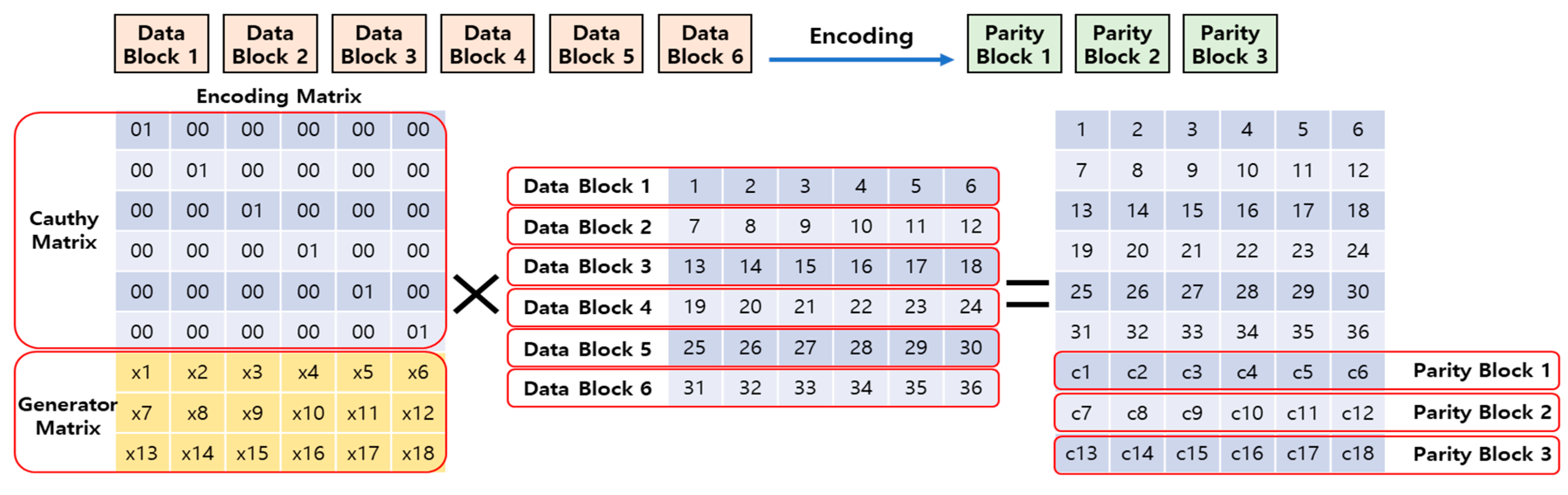
Figure 3 shows the encoding process in the EC-based distributed file system.
When encoding is performed on the RS (6, 3) volume, the original data are divided into six data blocks. The six divided data blocks generate three parity blocks through an encoding process. The encoding process is expressed in Equation (2), and the related notation is shown in
Table 3.
It is assumed that each piece of data of the six data blocks is composed of six items in a sequence. The generator matrix with three rows and six columns is created in a structure consistent with the RS (6, 3) volume used, and a parity block is generated by summing the values of each data block and the values of the corresponding rows and columns of the generator matrix. The generator matrix is composed of a partial matrix with zero and a generator matrix with three rows and six columns, which is determined using the Cauchy matrix, depending on the volume of RS (6, 3) [
15].
Figure 4 shows the decoding process of the EC-based distributed file system.
Errors have occurred in Data Block 3, Data Block 4, and Data Block 5, which need to be decoded. To do this, the corresponding row of the Cauchy matrix part used by Data Block 3, Data Block 4, and Data Block 5 must be deleted from the encoding matrix (Step 1). This generates an inverse matrix of the deleted encoding matrix, which is then multiplied on the left and right sides. The inverse matrix of the left side and the encoding matrix from which the error removed matrix are removed and are multiplied using the canceling out method (Step 2). Eventually, only the data composed of data blocks can be left, enabling the recovery of data blocks (Step 3). In other words, decoding involves calculating the inverse matrix through the encoding process of recovering the original data by using the previously written parity block. If expressed as a formula, the decoding process is shown in Equations (3)–(5), and the related notation is shown
Table 4.
During the decoding process, is obtained by removing the row corresponding to the error from the encoding matrix using Equation (3), and then the inverse matrix of , , is calculated. Next, is multiplied by both the left and right sides of the original encoding matrix using Equation (4). Finally, multiplying and using Equation (5) results in only , the data block that needs to be restored, remaining. This step uses the canceling out method to remove any unnecessary elements. Through this process, the decoding matrix is created by deleting the erroneous row from the encoding matrix, finding its inverse, and performing matrix multiplication.
4. Problem Analysis and Methodology Proposal
This section analyzes the problems that arise from the matrix used in encoding and decoding in EC-based distributed file systems. To solve these problems, the paper proposes a cache-based matrix technology.
4.1. Matrix Analysis for Encoding and Decoding
In an EC-based distributed file system, data are encoded and written into data blocks and parity blocks based on the EC volume used during the encoding process. Data can be read through decoding when no server failure occurs. In addition, in the event of a failure of the server, an inverse calculation can be performed by the EC algorithm to recover the data. When encoding and decoding instructions are executed, matrices are generated according to the set volume, which are used to store and recover data. In particular, the matrix required for the decoding process varies depending on several EC properties, including the EC algorithm used, the EC volume size, the location of the failed server, and the number of failed servers.
Figure 5 shows an example of a single server failure in a distributed file system configured with RS (6, 3) volumes.
Figure 5 shows a scenario where a single failure occurs among a total of nine servers, including servers that own Data Block 1 through Parity Block 3. When a decoding process is initiated for each server failure, a total of nine decoding matrices are generated, since a single failure occurs on nine servers. By calculating the number of cases when multiple failures occur, a total of 36 cases can be produced. The number of matrixes generated is equal to the number of failures allowed, which is the number of servers holding parity blocks, within the total number of servers. This can be expressed by Equation (6), which calculates the number of cases, and the related notation is shown in
Table 5 [
39].
For instance, if we calculate the triple failure of the RS (6, 3) volume, the result would be 84, which is equivalent to
9C3. In an EC distributed file system that is configured with RS (6, 3) volumes, up to three server failures can be tolerated, and a maximum of 84 decoding matrices can be generated. The calculation of the number of cases from a single failure to multiple failures in various forms of EC volume is expressed in
Table 6 by utilizing Equation (6).
Table 6 shows the maximum number of matrices that can be generated according to the number of server failures in the EC volume. When configured with RS (10, 4), a maximum of 1001 decoding matrices are generated from quadruple failure. However, generating all these matrices can result in unnecessary overhead. To address this issue, matrices that have the same structure as those used in previous encoding and decoding processes can be reused without having to create new ones. If these matrices are uploaded to cache memory, they can be accessed more quickly during encoding and decoding, which can help minimize unnecessary overhead.
4.2. Methodology of Cache-Based Matrix Technology
In order to upload a matrix to the cache memory and utilize it, the design of the cache memory is crucial. To implement the techniques proposed in this paper, the cache memory technique utilized is the WSCRP algorithm. The author has analyzed the problems associated with the replacement algorithm that is typically used in cache memory and proposed a new high-performance cache replacement algorithm called WSCRP, which is based on the WRP. WRP is an improved algorithm that builds on both LRU and LFU algorithms. The access time, which is an important performance indicator for cache memory, is faster than that of the main memory. To address this issue and efficiently improve cache memory access time, an adaptive replacement policy has been proposed. The adaptive replacement policy operates based on the LRU and LFU algorithms but assigns weights to each page based on specific parameters. These weights rank the pages based on their recentness, frequency, and reference rates. Additionally, since there is a reference rates parameter, a scheduling scheme in which a page with a low reference ratio is given higher priority is supported. In other words, the WRP algorithm prioritizes objects to be uploaded to the cache memory through weights and replaces low-ranking pages with new pages. Equation (7) shows the WRP algorithm, and the related notation is shown
Table 7.
If block j is in the buffer, a hit occurs in the cache memory, and the policy operates as follows if it is referenced:
will be changed to for every .
For , first we put , and then .
However, if the referenced block j is not in the buffer, a miss occurs, and the algorithm selects a block whose value of the weight function in the buffer is the highest among other values. When selecting, it searches for the object with the highest weight from the top to the bottom of the buffer, and if the weights of the objects are the same, the object that has been in the buffer for the longest time is selected for replacement. As a result, the weight values of the blocks in the buffer are updated on every access to the cache.
The WSCRP algorithm incorporates cost parameters into the adaptive replacement policy used in the WRP algorithm. Unlike the existing WRP algorithms, the WSCRP algorithm considers the size of the objects being replaced with cache memory when computing their weights. This prevents performance degradation that could occur based on the size of the objects being replaced. The weights of objects are calculated by adding cost parameters to the existing adaptive replacement policy. The WSCRP algorithm is shown in Equation (8), and the related notation is shown in
Table 8.
In the WSCRP algorithm, the parameter represents the object’s size, while the parameter is a cost value added to the adaptive replacement policy. The primary goal of the WSCRP algorithm is to save resources between the cache and the main memory. The cost value determines when an object is removed from the cache. As the cost value determines when an object is removed from the cache. As the cost value approaches that of all objects, the overall consumption can be calculated, and the cost of consuming a single object can be determined. If the replacement cost of any one object is higher, caching it can result in cost savings. In the case of an object, if the value is significant, it should be stored in the cache because it is more costly to perform a replacement and recache the cache. Therefore, this paper improves cache performance by adding the parameter to the existing Equation (7) to determine which object should be removed from the cache when the cache is full. The parameter takes up more cache space for extensive data, which may cause cache garbage to occur. This can result in unnecessary areas being freed up among the memory areas dynamically allocated by the program, thereby reducing the hit rate and increasing average access time. Therefore, it is best to prioritize caching small data. In addition, the parameter can save the replacement cost of an object because it replaces the data with a more significant weight value if the cost of replacing one piece of data is higher than another.
The cache memory table structure is sorted in ascending order according to the value calculated in Equation (8). If an object existing in the cache memory is searched and hit, the value is recalculated and rearranged in ascending order. In other words, objects with low values move up because they are likely to be referenced, and objects with high values move down because they are less likely to be referenced again. Therefore, if the value is more significant than that of other objects, this object is considered unimportant, and it is removed first when the cache memory is full. If an object with the same value exists, the parameter, which indicates the object’s reference rates, is used as the second attribute to determine the object to be removed from the cache.
Cache-based matrix technology operates based on the WSCRP algorithm and aims to maximize the hit rate to effectively use the matrix uploaded to the cache memory. When a request for a matrix is received, the system first checks the cache memory to see if the matrix exists for storing and recovering data. If a matrix is present in the cache memory for encoding and decoding, it is returned to the name node where the command was executed without generating a new matrix. However, if a matrix does not exist in the cache memory, the system considers it as a new instruction method, searches for currently available data nodes, creates a new matrix, returns it to the name node, and adds it to the cache memory. The
value of the uploaded matrix is then calculated using the weight–cost model, and the
value of the cache memory table structure is updated in ascending order. If there is insufficient space to store the matrix, the cache memory table alignment structure removes a matrix according to the update method until enough space is available to store the new data. The following Algorithm 1 shows the cache-based matrix technique.
| Algorithm 1: Cache-based matrix technology. |
| 1. | Parameter SCM: Calculates the size of the cache memory available |
| 2. | Parameter SRM: Calculates the size of the requested matrix |
| 3. | Parameter WC: Weight–cost values of matrix uploaded to cache memory |
| 4. | If the requested matrix exists in the cache |
| 5. | Find the matrix in the cache memory table |
| 6. | Update cache memory table |
| 7. | Else |
| 8. | Check the live data nodes |
| 9. | Available data nodes list transfer to name node |
| 10. | Create matrix |
| 11. | Add matrix to cache |
| 12. | While SCM < SRM |
| 13. | If there is only one maximum WC |
| 14. | Remove the maximum WC in the cache memory table |
| 15. | Else |
| 16. | Use frequency value to calculate and remove WC |
| 17. | Update cache memory table |
The algorithm for cache-based matrix technology first calculates the reference value through the weight–cost model when uploading to cache memory. It then calculates the free space of the cache memory, marks it as the size of cache memory (SCM), calculates the size of the matrix to be uploaded, and marks it as the size of the request matrix (SRM). If the name node performs encoding for data writing and decoding for reading and recovery, it checks whether the requested matrix exists in the cache memory. If it is present, the relevant matrix is found in the cache memory table, and encoding and decoding are performed through the matrix. The cache memory table is then updated by sorting the values of the used matrix in ascending order (Steps 3–5). If no matrix is found in the cache memory, a matrix must be generated. This is achieved by sending a list of available data nodes to the name node, which generates the matrix, uploads it to the cache, and performs encoding and decoding (Steps 6–10). If there is insufficient space in the cache memory to store the matrix, the algorithm removes the matrix with the maximum value through SCM and SRM. If there are multiple values, the algorithm removes the value, using frequency value as the second attribute (Steps 11–16).
4.3. Structure Design and CPU Performance of Cache-Based Matrix Technology
There are different architectural levels where caches can be located, but they are typically placed close to the front end to reduce the time and cost of accessing the backend service. Cache memory management methods can be classified into three types: centralized, global, and distributed cache structures. In a centralized structure, only one node can receive requests and access data. In a global structure, all nodes can access data using a single cache space. In a distributed cache structure, each node can access data using its own cache space. In this paper, the cache-based matrix technique employs a global structure where all data nodes use the cache space managed by the name node. The data node queries the name node for the matrix that encodes and decodes data, and the name node itself queries the storage space for data and delivers the matrices to the requested data node. If a distributed cache structure were used, each data node would manage its own matrix, which would lead to inefficient management due to the large number of resources, which would need to be managed by the name node. In addition, since the matrix is generated when the name node performs data writing, reading, and recovery operations, the probability of cache misses would be high if each data node managed its own matrix. Therefore, a global cache structure is advantageous because it allows the name node to generate and store the matrix through responses from multiple data nodes, thereby reducing cache misses.
The encoding and decoding operations involved in erasure coding can be computationally intensive and require a significant amount of CPU resources. Therefore, a faster CPU can generally perform these operations more quickly, which can improve the overall performance of the distributed file system. Different models of CPUs have different architectures and features that can affect their performance in various ways. For example, some CPU models may have more cores or higher clock speeds, which can help improve the performance of encoding and decoding operations. Additionally, different CPU models may have distinct instruction sets, which can affect the performance of specific algorithms used in erasure coding. However, it is worth noting that other factors, such as memory bandwidth, storage speed, and network bandwidth, can also impact erasure coding performance. Therefore, while CPU performance is an essential factor to consider, it is not the only one. Consequently, it is important to consider the specific model and characteristics of the CPU when designing and optimizing erasure coding algorithms for distributed file systems.
5. Experiments
This section introduces the experimental environment and results used in the evaluation. In this paper, we compare five systems: basic HDFS, the basic cache memory method LRU, HDFS with LFU applied, and HDFS with WRP and WSCRP applied, using the methodology described in
Section 4.
5.1. Experimental Environment
The algorithm described in
Section 4 was implemented using the Java programming language and operated as a simulation environment. The simulation of the cache-based matrix technology was conducted on a workstation running the Ubuntu 20.04.4 operating system, with a XEON 4110 (8 core × 2) CPU, 128 GB of DDR4 memory, a 20 TB (Terabyte) HDD Disk, and four RTX 2080 graphics cards. The version of Java Development Kit (JDK) used for development was 11.0.9, and the distributed file system that the cache-based matrix technology was applied to was HDFS. The version of Hadoop that includes HDFS is 3.3.2. The EC policy supported by HDFS includes RS and XOR algorithms, and it determines the number of data and parity blocks. The available EC policies were RS-3-2-1024k, RS-6-3-1024k, RS-10-4-1024k, RS-LEGACY-6-3-1024k, and XOR-2-1-1024k. In this paper, the RS algorithm was applied using RS-6-3-1024k. The data block was divided into six servers, and the parity block was divided into three servers, requiring a total of ten servers because a name node was also needed. The striping cell size is 1024k; this determines the granularity of reading and writing the stripe, including buffer size and encoding works. In an EC-based distributed file system, the size of a cell refers to the unit used when blocks are calculated and stored through encoding. The block cells are composed of 1024 kilobytes. A stripe is a single unit stored as a data block, encoded, and stored when generating a parity block. For instance, if Data Blocks 1, 2, 3, 4, 5, and 6 are encoded to generate Parity Blocks 1, 2, and 3, one stripe is composed of nine blocks.
The experimental method involved generating dummy data of 10 GB and writing the data using encoding commands. To generate a particular size of data, the fallocate command supported by Ubuntu was used, and the “−l” option was added to create a dummy data file with a size of 10 GB using the “fallocate −l 10g dummy data” command, which was then encoded and written. For decoding, file reading times were measured when data nodes did not fail, and recovery time was measured by randomly failing data nodes. In case of a random failure, the number of failed servers was not allowed to exceed the number of servers that wrote the parity blocks described in
Section 2. In other words, since there were a total of nine servers (six servers storing data blocks and three servers storing parity blocks), only single, double, and triple failures had been set up.
The experimental metrics measured the time taken to encode (write) and decode (read and recover) the data, and the hit rate of the cache memory followed Equation (9):
Five items were used for comparative analysis: basic HDFS RS (6, 3) without cache memory technology, HDFS RS (6, 3) with basic cache memory structure LRU and LFU, WRP HDFS RS (6, 3) based on WRP, and WSCRP HDFS RS (6, 3) proposed in this paper.
5.2. Experiments Result and Discussion
The experimental evaluation first shows the result of measuring the overhead of the matrix.
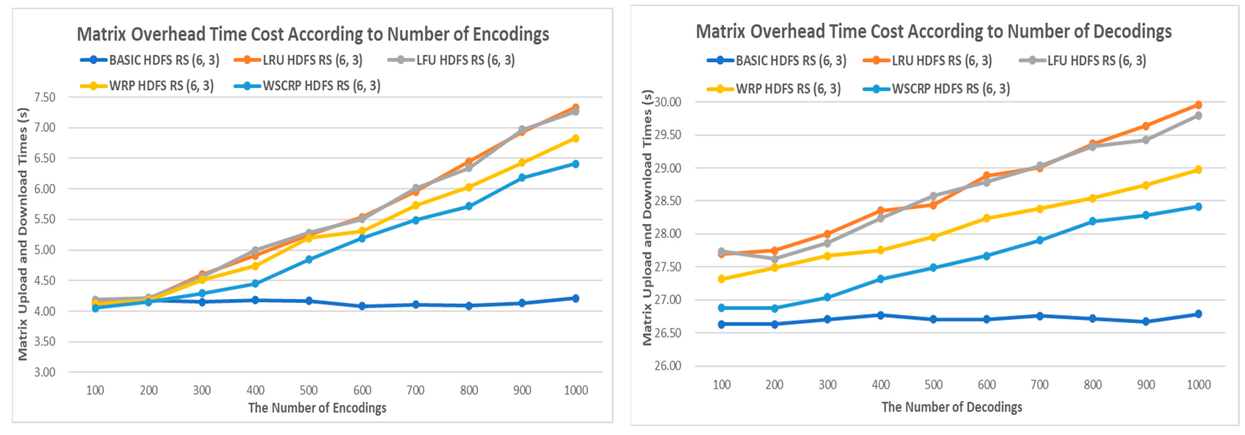
In
Figure 6, the time cost of uploading and downloading matrices generated during encoding and decoding to the cache memory is shown. As the number of encoding and decoding operations increases from 100 to 1000 times, the upload and download time of the matrix gradually increases. This is due to the increase in the number of matrices generated according to the number of encoding and decoding operations. However, the measurement time remains at around 4 s for the BASIC HDFS RS (6, 3) system, which does not utilize cache memory. Among the systems that utilize cache memory, the WSCRP HDFS RS (6, 3) system shows the lowest time cost, with a maximum encoding time of 6.4 s and a maximum decoding time of 28.4 s.
Figure 7 shows the space cost of the matrices stored in the cache memory. As the number of encodings and decodings increases, the matrices are cached, and the cache size increases gradually. The BASIC HDFS RS (6, 3) system does not utilize cache memory, and the initial measured size is maintained at approximately 14% during encoding and approximately 20% during decoding. However, among the systems that use cache memory, the WSCRP HDFS RS (6, 3) system can store more matrices as the number of encodings and decodings increases. The matrix size evaluated in terms of matrix overhead time and space cost is small at about 16 kilobytes. Although the time cost increases with an increasing number of encodings and decodings, it does not significantly affect the 1 Gbps network speed used in the experiment. Additionally, the space cost is sufficient to store the matrices, and systems utilizing cache memory can efficiently store the matrices through a replacement policy. Therefore, the costs of writing, reading, and recovering data are significantly affected, rather than the time and space cost of matrix overhead [
40].
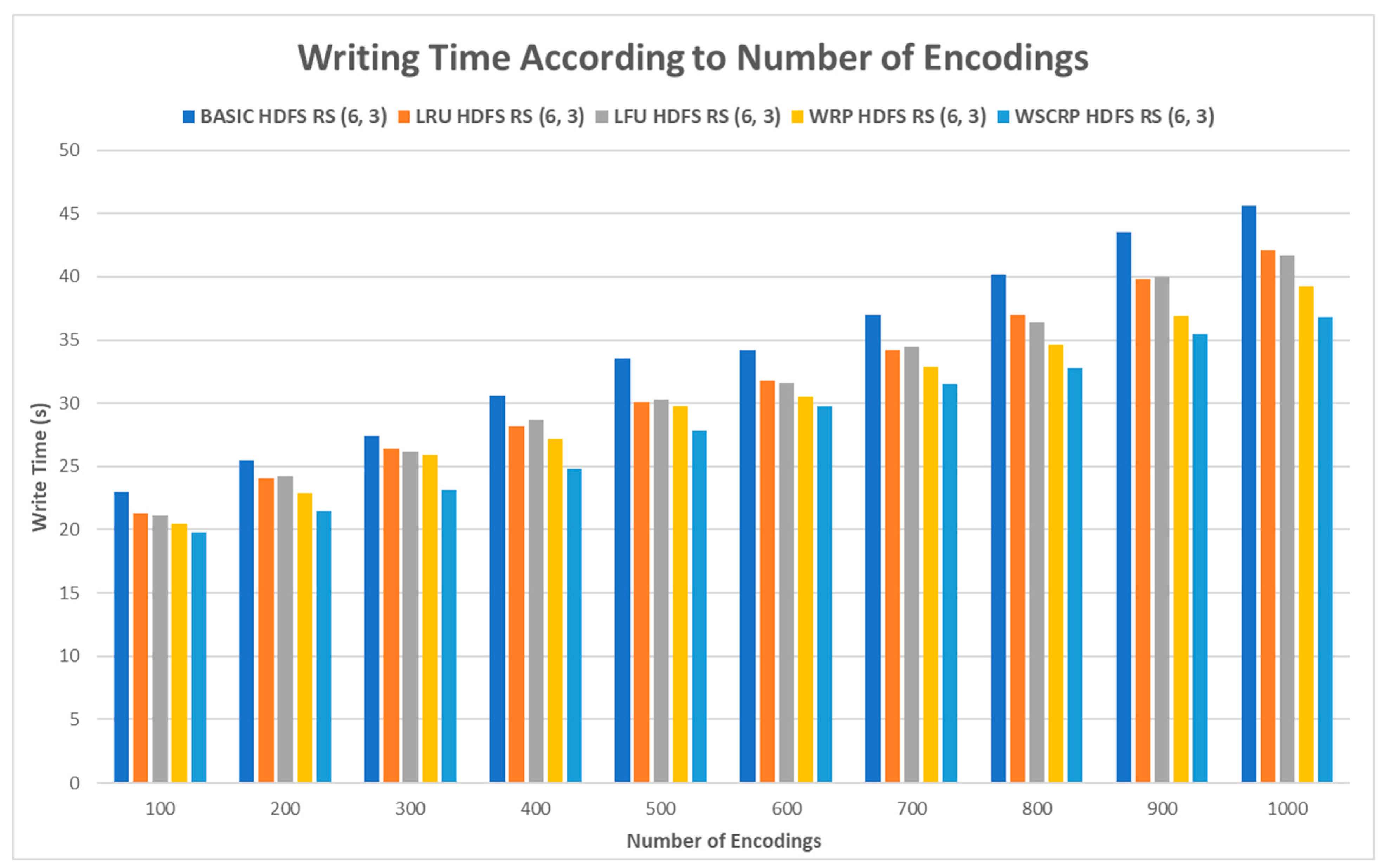
Figure 8 shows the writing time of encoding the generated data from 100 to 1000 times. As the number of encoding increases, the number of generated encoding matrices increases, so the overall writing time increases. Measurements from 100 to 1000 times showed that BASIC HDFS RS (6, 3) took 23 s to 45.6 s, LRU HDFS RS (6, 3) took 21.3 s to 42.1 s, and LFU HDFS RS (6, 3) took 21.1 s to 41.2 s. WRP HDFS RS (6, 3) took 19.9 s to 39.2 s, and WSCRP HDFS RS (6, 3) took 19.8 s to 36.8 s. When comparing BASIC HDFS RS (6, 3) with WSCRP HDFS RS (6, 3) based on 1000 encoding times, the writing time can be shortened by about 10 s. All the systems, except BASIC HDFS RS (6, 3), generate an encoding matrix, upload it to cache memory, and reuse the uploaded matrix for the next encoding, resulting in a small reduction in the overall writing time. In particular, WSCRP HDFS RS (6, 3) considering weights and parameters can save the most in writing time compared to LRU HDFS RS (6, 3) and LFU HDFS RS (6, 3) applying basic memory cache structures.
Figure 9 shows the reading time of decoding the encoded data from 100 to 1000 times. As the number of decodings increases, the number of generated decoding matrices increases, so the overall reading time increases. Measurements from 100 to 1000 times showed that BASIC HDFS RS (6, 3) took 285 s to 313.8 s, LRU HDFS RS (6, 3) took 282.8 s to 305.9 s, and LFU HDFS RS (6, 3) took 283.2 s to 304.2 s. WRP HDFS RS (6, 3) took 278.9 s to 295.8 s, and WSCRP HDFS RS (6, 3) took 270.5 s to 290.1 s. When comparing BASIC HDFS RS (6, 3) with WSCRP HDFS RS (6, 3) based on 1000 decoding times, the reading time can be shortened by about 23 s. All the systems, except BASIC HDFS RS (6, 3), generate a decoding matrix, upload it to cache memory, and reuse the uploaded matrix for the next decoding, resulting in a small reduction in overall reading time. In particular, WSCRP HDFS RS (6, 3) considering weights and parameters can save the most in reading time compared to LRU HDFS RS (6, 3) and LFU HDFS RS (6, 3) applying basic memory cache structures.
Figure 10 shows the recovery time measured when one to three nodes fail randomly, and decoding is performed 1000 times. When compared to the reading time in
Figure 9, where decoding was performed 1000 times without failure, the recovery time measured by the five systems gradually increases as the number of random node failures in
Figure 10 increases. This increase in decoding time is due to the selection of a data node that can respond, while excluding nodes with failures from the decoding matrix calculation. Among the five systems, WSCRP HDFS RS (6, 3) shows the shortest recovery time, measuring 296.1 s for a single failure of a random node, 305.3 s for double failures of a random node, and 336.8 s for triple failures of a random node, making it the most efficient system among the five.
The results of measuring writing and reading time by performing encoding and decoding without any failure show that the number of matrices used is reduced. However, as the maximum number of executions approaches 1000, both the writing and recovery times gradually increase. This is because although the number of matrices used is smaller than the number used in the presence of failures, the number of matrices increases with the number of encodings and decodings, which in turn results in an increase in writing and reading time [
41].
Figure 11 shows the hit rate of the matrix that was uploaded to and accessed from the cache memory. During the experiment shown in
Figure 11, the hit rate was measured every 100 times while the recovery time of the random triple node failure (the third item in
Figure 10) was being evaluated.
BASIC HDFS RS (6, 3) does not upload the matrix generated by the decoding process to the cache memory. As a result, the hit rate remains around 10% even as the number of decodings increases. In contrast, the remaining four systems reuse the matrix uploaded to the cache memory, causing the hit rate to gradually increase with the number of decodings. The number of decodings increases rapidly up to 600. However, from 600 decodings onwards, the hit rate increases only slightly compared to the previous values. This is because, at 600 decodings, the cache memory is full and the page replacement policy is triggered. When the number of decodings reaches 1000, the hit rates of LRU HDFS RS (6, 3) and LFU HDFS RS (6, 3) show little difference, measuring at 73.8% and 73.2%, respectively. The hit rate of WRP HDFS RS (6, 3) is slightly superior to the LRU and LFU structures, measuring at 75.4%. As the number of decodings increases, the hit rate of WSCRP HDFS RS (6, 3) is measured to be higher than that of WRP HDFS RS (6, 3). It reaches its best value of 83.8% at 1000 decodings.
6. Conclusions and Future Directions
This paper proposes a cache-based matrix technique, which is a method for efficiently utilizing symmetrical space in EC-based distributed file systems. The technique uses the encoding used for file writing and the matrix generated when performing decoding used for file reading and recovery. Up to 1001 matrices based on the RS (10, 4) volume were generated, depending on the server that failed during file writing, reading, and recovery. Cache-based matrix technology can maintain a high cache memory hit rate, which can shorten file storage and recovery times during encoding and decoding. Additionally, since cache memory is utilized in terms of software, there is no cost to adding or changing hardware modules. The WSCRP algorithm underlying this technology can efficiently handle the page replacement policy of cache memory through weights and cost parameters. Therefore, this paper focuses on using matrices to reduce overhead in distributed file systems.
Future research directions are organized into three directions. First, the proposed technology will be applied not only to RS (6, 3), but also to various volumes of RS (3, 2), RS (8, 4), and RS (10, 4). Second, the proposed technology will be applied not only to HDFS but also to Ceph and GlusterFS, which are distributed file systems that support the EC algorithm. Finally, we will analyze the data blocks, parity blocks, and matrices that change when data are updated in the distributed file system. We plan to study how to reduce the overhead that occurs when updating data, as well as writing, reading, and recovering data.


