Analytical Solutions of Peristalsis Flow of Non-Newtonian Williamson Fluid in a Curved Micro-Channel under the Effects of Electro-Osmotic and Entropy Generation

Abstract

In the current effort, the effects of entropy generation and electro-osmotic driven peristaltic flow of non-Newtonian Williamson liquid in a curved micro-channel is investigated. Formulation of the problem is conducted in a wave frame of reference. Due to the complexity of non-Newtonian fluid, the analytical solutions of non-linear coupled equations are not easy to obtain and are very rarely found in the literature. For analytical solutions, the governing equations are reduced in the form of the Bessel function. The electric double layer is employed as a result of a zeta potential of about 25 mV. The low Reynolds number and long wavelength approximations are taken into account. Graphical analysis has been carried out for velocity, temperature and entropy for physical parameters. It is noted that the Brinkmann number enhances the temperature. The results of this model will be extremely helpful in designing electro-peristaltic pumps for thermal systems.

1. Introduction

Peristalsis is derived from the Greek term peristaltikos, which means to clutch and compress. It is a known fact that a peristaltic wave propagating along the pliable walls of a tube/channel can push small particles suspended in fluid even without an external pressure gradient. The reproductive system of males and females is a good example. Urine motion from the kidney to the bladder via the ureter is another excellent example of peristalsis in the human body. In a human’s digestion in which a peristaltic wave is stimulated by muscles to move the swallowed food to the stomach via the esophagus can also can be mentioned. In engineering, peristalsis include designing roller pumps, breaker and handle pumps and other fluid-handling devices. Toxic liquid is transported using this method in the nuclear sector to prevent contamination. On peristaltic flow under diverse aspects, the first attempt was performed by Latham [1] in this direction. Jaffrin and Shapiro [2] extended the work of Latham. After then, various authors [3,4,5,6,7,8] have examined the peristalsis due to its significance in biomedical and industrial studies.

Moreover, electro kinetic concerns the flow of ionic fluid. When this electro kinetic process occurs in a membrane, micro-channel or porous material is called electro-osmotic process. Major biological uses of electro-osmosis involve implantable neuroprobes, cell cultures, cellular micro-infection, etc. Chakraborty [9] first analyzed the peristaltic flow with the electro-osmotic effect. Tripathi et al. [10] debated the electro-osmotic peristaltic movement in a micro-channel with Joule heating. Narla et al. [11] discussed the electro-osmotic effect on viscous liquid through a wavy micro-channel. Khan et al. [12] explained the peristaltic movement in a curved channel with electro-osmosis. They found that the temperature rises by increasing double layer thickness. Major investigation in the refs [13,14,15,16] have studied the electro-osmotic effect in a curved channel with peristalsis.

Furthermore, entropy is recognized as thermal irreversibility or a reduction in valuable energy. It is one of the main problems for investigators to accomplish the reduction of thermal energy. In thermo-dynamical systems, viscosity and frictional forces are the key reasons of energy degradation. Firstly, Bejan [17,18] worked on entropy generation. Later, numerous scientists have also considered irreversibility analysis and established its efficacy to find out the effectiveness of the system. Jhorar et al. [19] considered electro osmosis effects on through asymmetric microfluidics channel. Ellahi et al. [20] examined the effects of electro-osmotic and entropy generation on power-law fluid. Few most pertinent investigations can be seen in [21,22,23,24,25].

The two-dimensional characteristics-based scheme for energy and Navier–Stokes equations are presented for the first time by Rostamzadeh et al. [26]. The main purpose of the scheme is to solve the incompressible flows in complex geometries. Trabzon et al. [27] goals to simulate the active electrohydrodynamic-based micromixer for the high-throughput formation of nanoscale liposomes. Sharma et al. [28] studied the motion of motile gyrotactic micro-organisms in polyvinyl alcohol–water with solar radiation and the entropy generation effects. Gandhi et al. [29] deliberated blood movement through a stenotic artery affected by the Joule heating, a viscous dissipation electric field, radiation and a magnetic field. KKL correlations and other parameters are introduced in the first part. KKL correlations are used for the simulation of nanofluid. Sridhar et al. [30] deliberated the influence of hybrid nanoparticles on couple stress fluid in a vertical micro-channel.

To the best of authors’ knowledge, the peristaltic flow of Williamson fluid in a curved channel under the simulation effects of electro-osmotic and entropy generation has not been investigated previously. The current effort is devoted to fill the said gape in the existing literature. The stream functions are used to model the problem. The resulting problem is non-dimensionalized using the lubrication approximation theory at a low Reynolds number and long wavelength. The analytical solution is established in terms of the Bessel function. The ND Solver command is used to solve the resulting equations. The variation in several parameters can be examined graphically.

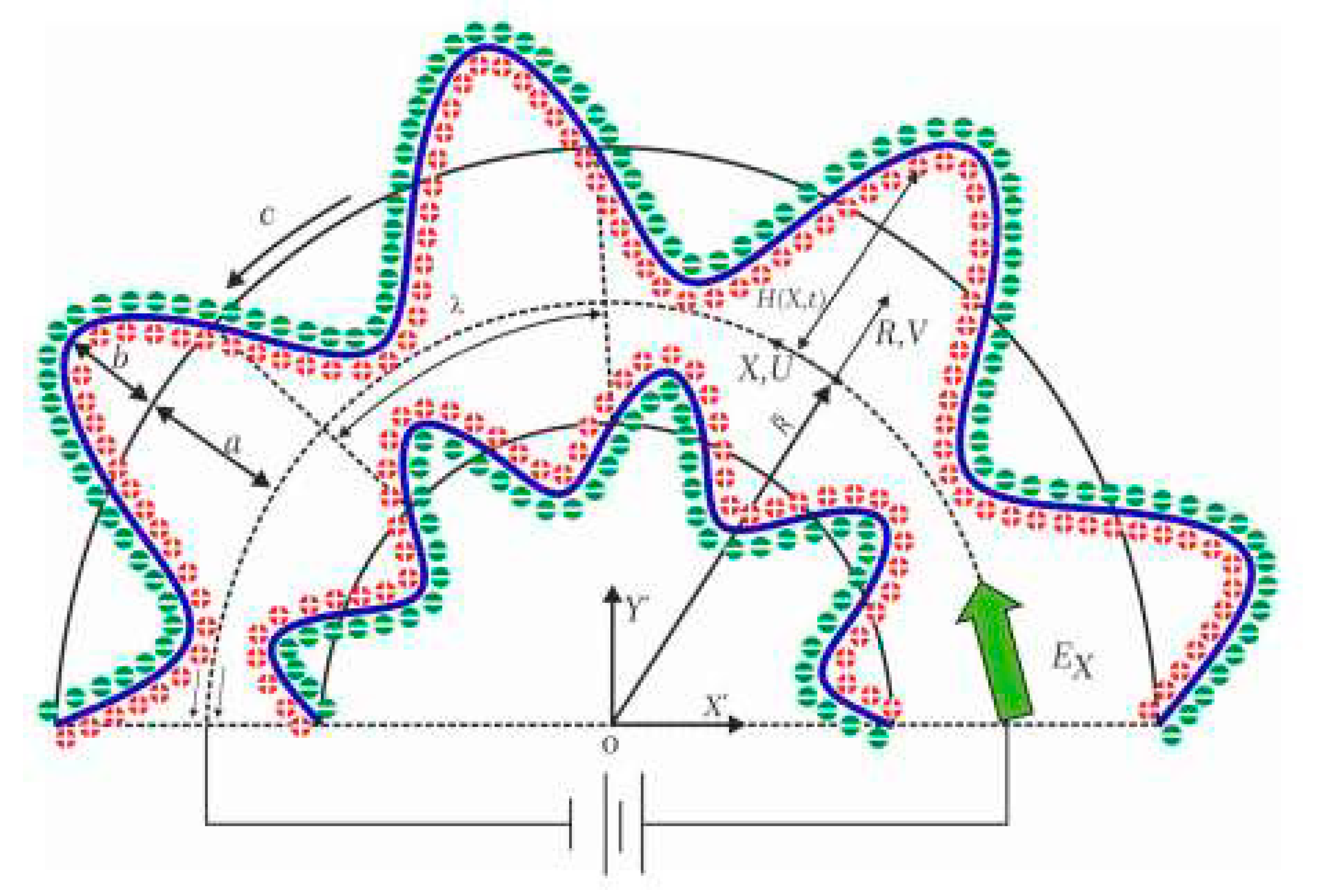
2. Problem Formulation

The peristaltic motion of Williamson fluid in a curved configuration with a width 2$a$ loop in a circle with a center $O$ and a curvature radius of $R$ is considered. The time-dependent wall fluid interface is represented as

$$\overline{R}=\pm \overline{H}\left(\overline{X},\overline{t}\right)=\pm a\mp b {cos}^2\left(\pi \left(\frac{\overline{X}}{\lambda }-\frac{\overline{t}}{\tau }\right)\right),$$

(1)

where $b$ the wave’s amplitude, $H$ the wave’s radial displacement from the center line, $\lambda$ the wave’s length, $\tau$ the wave’s period and $t$ the time. The half width of the channel is modest in comparison to the wavelength $\left(a\ll \lambda \right)$ as shown in Figure 1.

The following are the basic equations for a fluid flow field given as [31,32]

$$\nabla .{\mathit{V}}^{\prime }=0,$$

(2)

$$\rho \left[\frac{\partial {\mathit{V}}^{\prime }}{\partial \overline{t}}+\left({\mathit{V}}^{\prime }.\nabla \right){\mathit{V}}^{\prime }\right]=-\nabla \overline{P}+{\mu }_0\left[1+\mathsf{\Gamma }\dot{\mathsf{{\rm Y}}}\right]{\acute{\mathit{A}}}_1+{\rho }_e\overline{\mathit{E}},$$

(3)

where ${\acute{\mathit{A}}}_1=\nabla {\mathit{V}}^{\prime }+{\left(\nabla {\mathit{V}}^{\prime }\right)}^T$ $\dot{\gamma }=\sqrt{\frac{1}{2}\pi }$, $\pi =trace\stackrel{´}{{{\mathit{A}}^2}_1}$.

${\mathit{V}}^{\prime }=\overline{U}\left(\overline{X},\overline{R},\overline{t}\right){\widehat{e}}_{\overline{X}}+\overline{V}\left(\overline{X},\overline{R},\overline{t}\right){\widehat{e}}_{\overline{R}}$ the velocity vector, ${\mu }_0$ and $\rho$ the viscosity and density of the fluid. $\overline{\mathit{E}}$ represent electric field and ${\rho }_e=ez\left(n_{+}+n_{-}\right)$ denotes the net charge density of permittivity $\epsilon$, $n_{\pm }$ denoting the number densities of p-ions, $z$ denoting the ionic valence and $\overline{P}$ is pressure. Equations (1) and (2) in component form are given below:

$$R^{\prime }\frac{\partial \overline{U}}{\partial \overline{X}}+\frac{\partial }{\partial \overline{R}}\left\{\left(\overline{R}+R^{\prime }\right)\overline{V}\right\}=0,$$

(4)

$$\frac{{\overline{U}R}^{\prime }}{\left(R^{\prime }+\overline{R}\right)}\frac{\partial \overline{U}}{\partial \overline{X}}+\overline{V}\frac{\partial \overline{U}}{\partial \overline{R}}+\frac{\overline{U}\overline{V}}{R^{\prime }+\overline{R}}+\frac{\partial \overline{U}}{\partial \overline{t}}={\rho }_e{\overline{E}}_{\overline{X}}-\frac{R^{\prime }}{\rho \left(R^{\prime }+\overline{R}\right)}\frac{\partial \overline{P}}{\partial \overline{X}}+\nu \left[\frac{1}{{\left(R^{\prime }+\overline{R}\right)}^2}\frac{\partial }{\partial \overline{R}}\left[{\left(R^{\prime }+\overline{R}\right)}^2{\overline{\tau }}_{\overline{R}\overline{X}}\right]+\frac{R^{\prime }}{R^{\prime }+\overline{R}}\frac{\partial {\overline{\tau }}_{\overline{X}\overline{X}}}{\partial \overline{X}}\right],$$

(5)

$$\overline{V}\frac{\partial \overline{V}}{\partial \overline{R}}+\frac{\partial \overline{V}}{\partial \overline{t}}+\frac{R^{\prime }\overline{U}}{\left(R^{\prime }+\overline{R}\right)}\frac{\partial \overline{V}}{\partial \overline{X}}-\frac{{\overline{U}}^2}{R^{\prime }+\overline{R}}=-\frac{1}{\rho }\frac{\partial \overline{P}}{\partial \overline{R}}+v\left[\frac{1}{R^{\prime }+\overline{R}}\frac{\partial }{\partial \overline{R}}\left[\left(R^{\prime }+\overline{R}\right){\overline{\tau }}_{\overline{R}\overline{R}}\right]+{\rho }_e{\overline{E}}_{\overline{R}}+\frac{R^{\prime }}{R^{\prime }+\overline{R}}\frac{\partial {\overline{\tau }}_{\overline{R}\overline{X}}}{\partial \overline{R}}-\frac{1}{R^{\prime }+\overline{R}}{\overline{T}}_{\overline{X}\overline{X}}\right].$$

(6)

The heat transfer equation is as follows

$$\rho C_P\frac{\mathrm{d}\overline{T}}{\mathrm{d}\overline{t}}=K\left[\frac{\partial }{\partial \overline{R}}\left(\frac{\partial \overline{T}}{\partial \overline{R}}\right)-\frac{\kappa }{\overline{R}+R^{\prime }}\frac{\partial \overline{T}}{\partial \overline{R}}+\frac{\partial }{\partial X}\left(\frac{R^{\prime 2}}{{\left(\overline{R}+R^{\prime }\right)}^2}\frac{\partial \overline{T}}{\partial \overline{R}}\right)\right]+{\sigma }_e{{\overline{E}}_{\overline{X}}}^2-\frac{\partial \overline{V}}{\partial \overline{R}}\left(-{\overline{\tau }}_{\overline{R}\overline{R}}+{\overline{\tau }}_{\overline{X}\overline{X}}\right)+{\overline{\tau }}_{\overline{R}\overline{X}}\left(\frac{R^{\prime }}{R^{\prime }+\overline{R}}\frac{\partial \overline{V}}{\partial \overline{X}}+\frac{\partial \overline{U}}{\partial \overline{R}}-\frac{\overline{U}}{R^{\prime }+\overline{R}}\right),$$

(7)

with the boundary conditions

$$\overline{V}=0,\overline{T}=T_0 at \overline{R}=-\overline{H}\mathrm{and}\overline{T}=T_0, \overline{V}=0, at \overline{R}=\overline{H},$$

(8)

where $T_0$ is the absolute.

Bulk fluid motion can cause electro-osmotic flow to occur. The electro-osmotic flow relationship can be written as:

$$\overline{\mathit{E}}={\overline{E}}_{\overline{X}}{\widehat{e}}_{\overline{X}}+{\overline{E}}_{\overline{R}}{\widehat{e}}_{\overline{R}}=-\nabla \overline{\Phi }=-\frac{R^{\prime }}{R^{\prime }+\overline{R}}\frac{\partial \overline{\Phi }}{\partial \overline{X}}{\widehat{e}}_{\overline{X}}-\frac{\partial \overline{\Phi }}{\partial \overline{R}}{\widehat{e}}_{\overline{R}},$$

(9)

where electric potential function is $\overline{\Phi }$. The Poisson equation is used to explain the charge number density associated with electric potential.

$${\nabla }^2\overline{\Phi }=\frac{R^{\prime 2}}{{\left(R^{\prime }+\overline{R}\right)}^2}\frac{{\partial }^2\overline{\Phi }}{\partial {\overline{X}}^2}+\frac{1}{R^{\prime }+\overline{R}}\frac{\partial }{\partial \overline{R}}\left\{\left(R^{\prime }+\overline{R}\right)\frac{\partial \overline{\Phi }}{\partial \overline{R}}\right\}=-\frac{{\rho }_e}{\epsilon }.$$

(10)

According to the wall’s asymmetric zeta potential is defined as:

$$\overline{\Phi }\left(-\overline{H}\right)={\overline{\zeta }}_1,\overline{\Phi }\left(\overline{H}\right)={\overline{\zeta }}_2.$$

(11)

In the absence of a chemical reaction, the Nernst–Planck equation (an equation for the conservation of mass is used to explain how a charged chemical species moves through a fluid. It is used to compute the minimal amount of energy needed for electro-dialysis) is expressed as follows:

$$\left(\frac{\partial {\overline{n}}_{\pm }}{\partial \overline{t}}+\overline{U}\frac{R^{\prime }}{R^{\prime }+\overline{R}}\frac{\partial {\overline{n}}_{\pm }}{\partial \overline{X}}+\overline{V}\frac{\partial {\overline{n}}_{\pm }}{\partial \overline{R}}\right)={\overline{D}}_{\pm }\left({\nabla }^2{\overline{n}}_{\pm }\right)\pm \frac{{\overline{D}}_{\pm }{z}_{\pm }e}{{\kappa }_B{T}_0}\left[\frac{R^{\prime }}{R^{\prime }+\overline{R}}\frac{\partial }{\partial \overline{X}}\left\{{\overline{n}}_{\pm }\frac{R^{\prime }}{R^{\prime }+\overline{R}}\frac{\partial \overline{\Phi }}{\partial \overline{X}}\right\}+\frac{1}{R^{\prime }+\overline{R}}\frac{\partial }{\partial \overline{R}}\left\{\left(R^{\prime }+\overline{R}\right)n_{\pm }\frac{\partial \overline{\Phi }}{\partial \overline{R}}\right\}\right],$$

(12)

where $\overline{D}$ is ionic species diffusivity and ${\kappa }_B$ is the Boltzmann constant.

Transformation between a wave and a fixed frame for simplification is as follows:

$$x^{\prime }=\overline{X}-c\overline{t},r^{\prime }=\overline{R},v^{\prime }=\overline{V},\overline{h}\left(\overline{x}\right)=\pm a\mp b{cos}^2\left(\frac{\pi \overline{x}}{\lambda }\right),u^{\prime }=\overline{U}-c,\overline{p}\left(\overline{x},\overline{r}\right)=\overline{P}\left(\overline{X},\overline{R}\right),$$

In the lab frame, $\overline{U},\overline{V}$ are components of velocity, while in the wave frame, $\overline{u},\overline{v}$ are velocity components. To non-dimensionalize our problem, the transformation below is described.

$$\begin{array}{l}\overline{x}=\frac{x^{\prime }}{\lambda },\overline{v}=\frac{v^{\prime }}{\delta c},\overline{h}=\frac{\overline{h}}{a},\overline{\Phi }=\frac{b}{a},k=\frac{R^{\prime }}{a},L^{\prime }=\frac{\overline{L}}{\lambda },\overline{p}=\frac{a^2\overline{P}}{\mu c\lambda },Re=\frac{ca\delta }{\nu },\overline{\psi }=\frac{{\psi }^{\prime }}{ac},\overline{F}=\frac{Q}{ac},r^{\prime }=\frac{r^{\prime }}{a},\\ m^{\prime }=\overline{m}a,{\Phi }^{\prime }=\frac{\overline{\Phi }}{{\Phi }_0},\overline{v}=-\frac{k}{\overline{r}+k}\frac{\partial \overline{\psi }}{\partial \overline{x}},{\zeta }_1=\frac{{\overline{\zeta }}_1}{{\Phi }_0},{\zeta }_2=\frac{{\overline{\zeta }}_2}{{\Phi }_0},U_{HS}=\frac{{\overline{U}}_{HS}}{c},Pe=\frac{c\lambda }{\overline{D}},n^{\prime }=\frac{n}{n_0},c=\frac{\lambda }{\tau },\delta =\frac{a}{\lambda },\\ {\Phi }_0=\frac{{\kappa }_B{T}_0}{e_z},\overline{u}=\frac{u^{\prime }}{c},\theta =\frac{T-T_0}{T_0},U_{HS}=-\frac{\epsilon {\Phi }_0{\overline{E}}_x}{\mu },B_r=\frac{\mu c^2}{K{T}_0},P_r=\frac{C_p\mu }{K},\overline{u}=\frac{\partial \overline{\psi }}{\partial \overline{r}},We=\frac{\mathsf{\Gamma }c}{L},S=\frac{{{\sigma }_e{{\overline{E}}_{\overline{x}}}^{2}a}^2}{k{T}_0},\end{array}$$

(13)

With the usage of Equation (9) as ${\overline{E}}_{\overline{r}}~\delta {\overline{E}}_{\overline{x}}\frac{k}{k+\overline{r}}$ along the boundary conditions and employing stream functions.

The Equations (5)–(7) and the Poisson Equation (10) wave frame become

$$\begin{array}{l}Re\delta \left[-\frac{1}{k}\frac{{\partial }^2\overline{\psi }}{\partial \overline{x}\partial \overline{r}}+\frac{1}{\overline{r}+k}\frac{\partial \overline{\psi }}{\partial \overline{x}}\frac{{\partial }^2\overline{\psi }}{\partial {\overline{r}}^2}-\frac{1}{{\left(\overline{r}+k\right)}^2}\left(\frac{\partial \overline{\psi }}{\partial \overline{r}}+1\right)\frac{\partial \overline{\psi }}{\partial \overline{x}}+\frac{1}{\overline{r}+k}\left(\frac{\partial \overline{\psi }}{\partial \overline{r}}+1\right)\frac{{\partial }^2\overline{\psi }}{\partial \overline{x}\partial \overline{r}}-\frac{\overline{r}+k}{k}\frac{{\partial }^3\overline{\psi }}{\partial \overline{x}\partial {\overline{r}}^2}-\frac{\partial \overline{\psi }}{\partial \overline{x}}\frac{{\partial }^3\overline{\psi }}{\partial {\overline{r}}^3}+\frac{\overline{r}+k}{k}\left(\frac{\partial \overline{\psi }}{\partial \overline{r}}+1\right)\frac{\partial }{\partial {\overline{r}}^2}\left[\frac{k}{\overline{r}+k}\frac{\partial \overline{\psi }}{\partial \overline{x}}\right]\right]\\ =-\frac{{\partial }^2\overline{p}}{\partial \overline{x}\partial \overline{r}}+\delta \frac{{\partial }^2{\overline{\tau }}_{\overline{x}\overline{x}}}{\partial \overline{x}\partial \overline{r}}+\frac{\partial }{\partial \overline{r}}\left[\frac{1}{k\left(\overline{r}+k\right)}\frac{\partial }{\partial \overline{r}}{\left(\overline{r}+k\right)}^2{\overline{\tau }}_{\overline{r}\overline{x}}\right]+U_{HS}\left[-\frac{k{\delta }^2}{{\left(\overline{r}+k\right)}^2}\frac{{\partial }^2\overline{\Phi }}{\partial {\overline{x}}^2}+\frac{k{\delta }^2}{\left(\overline{r}+k\right)}\frac{{\partial }^3\Phi }{\partial {\overline{x}}^2\partial \overline{r}}+\frac{2}{k}\frac{{\partial }^2\Phi }{\partial {\overline{r}}^2}+\frac{\overline{r}+k}{k}\frac{{\partial }^3\Phi }{\partial {\overline{r}}^3}\right],\end{array}$$

(14)

$$\begin{array}{l}Re\delta \left[\frac{k{\delta }^2}{\left(\overline{r}+k\right)}\frac{{\partial }^3\overline{\psi }}{\partial {\overline{x}}^3}-\frac{2k^2{\delta }^2}{{\left(\overline{r}+k\right)}^3}\frac{{\partial }^2\overline{\psi }}{\partial {\overline{x}}^2}\frac{\partial \overline{\psi }}{\partial \overline{x}}+\frac{k^2{\delta }^2}{{\left(\overline{r}+k\right)}^2}\frac{\partial \overline{\psi }}{\partial \overline{x}}\frac{{\partial }^3\overline{\psi }}{\partial {\overline{x}}^2\partial \overline{r}}-\frac{k^2{\delta }^2}{{\left(\overline{r}+k\right)}^2}\left(\frac{\partial \overline{\psi }}{\partial \overline{r}}+1\right)\frac{{\partial }^3\overline{\psi }}{\partial {\overline{x}}^3}+\frac{2}{\overline{r}+k}\left(\frac{\partial \overline{\psi }}{\partial \overline{r}}+1\right)\frac{{\partial }^2\overline{\psi }}{\partial \overline{x}\partial \overline{r}}\right]\\ =-\frac{{\partial }^2\overline{p}}{\partial \overline{x}\partial \overline{r}}-\frac{\delta }{\left(\overline{r}+k\right)}\frac{{\partial }^2{\overline{\tau }}_{\overline{x}\overline{x}}}{\partial \overline{x}}+\frac{k{\delta }^2}{\left(\overline{r}+k\right)}\frac{{\partial }^2{\overline{\tau }}_{\overline{r}\overline{x}}}{\partial {\overline{x}}^2}+\frac{\delta }{\left(\overline{r}+k\right)}\frac{{\partial }^2}{\partial \overline{x}\partial \overline{r}}\left[\left(\overline{r}+k\right){\overline{\tau }}_{\overline{r}\overline{r}}\right]\\ +U_{HS}\frac{\delta k}{\left(\overline{r}+k\right)}\left[\frac{k^2{\delta }^3}{{\left(\overline{r}+k\right)}^2}\frac{{\partial }^3\Phi }{\partial {\overline{x}}^3}+\frac{1}{\left(\overline{r}+k\right)}\delta \frac{\partial }{\partial \overline{r}}\left\{\left(\overline{r}+k\right)\frac{{\partial }^2\Phi }{\partial \overline{x}\partial \overline{r}}\right\}\right],\end{array}$$

(15)

$$\begin{array}{l}Re{P}_r\delta \left[\frac{\partial }{\partial \overline{t}}+\left(\frac{\partial \overline{\psi }}{\partial \overline{r}}+1\right)\frac{k}{\left(\overline{r}+k\right)}\frac{\partial }{\partial \overline{x}}-\frac{k}{\left(\overline{r}+k\right)}\frac{\partial \overline{\psi }}{\partial \overline{x}}\frac{\partial }{\partial \overline{r}}\right]\theta \\ =\left[\frac{{\partial }^2}{\partial r^2}-\frac{1}{\left(\overline{r}+k\right)}\frac{\partial }{\partial \overline{r}}+\frac{k^2}{{\left(\overline{r}+k\right)}^2}\frac{{\partial }^2}{\partial x^2}{\delta }^2\right]\theta +S+B_r\delta \frac{\partial }{\partial \overline{r}}\left(\frac{\partial \overline{\psi }}{\partial \overline{r}}\right)\left({\overline{\tau }}_{\overline{x}\overline{x}}-{\overline{\tau }}_{\overline{r}\overline{r}}\right)\\ +B_r\left({\delta }^2\frac{k}{\left(\overline{r}+k\right)}\frac{\partial }{\partial \overline{x}}\left(\frac{-k}{\left(\overline{r}+k\right)}\frac{\partial \overline{\psi }}{\partial \overline{x}}\right)+\frac{{\partial }^2\overline{\psi }}{\partial {\overline{r}}^2}-\left(\frac{\partial \overline{\psi }}{\partial \overline{r}}+1\right)\frac{1}{\left(\overline{r}+k\right)}\right){\overline{\tau }}_{\overline{r}\overline{x}},\end{array}$$

(16)

$${\delta }^2{\left(\frac{k}{\overline{r}+k}\right)}^2\frac{{\partial }^2\Phi }{\partial {\overline{x}}^2}+\frac{{\partial }^2\Phi }{\partial {\overline{r}}^2}+\frac{1}{\overline{r}+k}\frac{\partial \Phi }{\partial \overline{r}}+m^2\left(\frac{n_{+}-n_{-}}{2}\right)=0.$$

(17)

After non-dimensionalization, Equation (11) is written as:

$$\Phi \left(-\overline{h}\right)={\zeta }_1,\Phi \left(\overline{h}\right)={\zeta }_2.$$

(18)

The non-dimensionalized form of Equation (12) is:

$$\begin{array}{l}Pe{\delta }^2\left[\left(\frac{\partial \overline{\psi }}{\partial \overline{r}}+1\right)\frac{k}{k+\overline{r}}\frac{\partial n_{\pm }}{\partial \overline{x}}-\frac{k}{\left(\overline{r}+k\right)}\frac{\partial \overline{\psi }}{\partial \overline{x}}\frac{\left(\partial n_{\pm }\right)}{\partial \overline{r}}\right]=\left({\delta }^2{\left(\frac{k}{\overline{r}+k}\right)}^2\frac{{\partial }^2{n}_{\pm }}{\partial {\overline{x}}^2}+\frac{{\partial }^2{n}_{\pm }}{\partial {\overline{r}}^2}+\frac{1}{\overline{r}+k}\frac{\partial n_{\pm }}{\partial \overline{r}}\right)\pm \\ \left({\delta }^2\frac{k}{k+\overline{r}}\frac{\partial }{\partial \overline{x}}\left\{\frac{k}{k+\overline{r}}{n}_{\pm }\frac{\partial \Phi }{\partial \overline{x}}\right\}+\frac{1}{k+\overline{r}}\frac{\partial }{\partial \overline{r}}\left\{\left(k+\overline{r}\right)n_{\pm }\frac{\partial \Phi }{\partial \overline{r}}\right\}\right).\end{array}$$

(19)

where $Pe=ReSc,$ $Re$ is the Reynolds number and $Sc$ is the Schmidt number. We are adopting long wave length and low Reynolds approximation which is valid in peristaltic wave propagation. Therefore, ${\delta }^2\to 0$ and $Pe{\delta }^2\to 0$. Equation (19) becomes

$$\left(\frac{1}{\overline{r}+k}\frac{\partial n_{\pm }}{\partial \overline{r}}+\frac{{\partial }^2{n}_{\pm }}{\partial {\overline{r}}^2}\right)\pm \frac{1}{k+\overline{r}}\frac{\partial }{\partial \overline{r}}\left\{\left(k+\overline{r}\right)n_{\pm }\frac{\partial \Phi }{\partial \overline{r}}\right\}=0,$$

(20)

According to condition $n_{\pm }\left(\Phi =0\right)=1$ and $\frac{\partial n_{\pm }}{\partial \overline{r}}=0$ where $\frac{\partial \Phi }{\partial \overline{r}}=0,$ consequently, we obtain Boltzmann distributions for ions that are

$$n_{\pm }=exp\left(\mp \Phi \right).$$

(21)

Now, we will use Equation (20) and apply the condition $\left(\delta \to 0\right)$ in Equation (17)

$$\frac{{\partial }^2\Phi }{\partial {\overline{r}}^2}+\frac{1}{\overline{r}+k}\frac{\partial \Phi }{\partial \overline{r}}=m^2\sinh \Phi .$$

(22)

Now, subtracting Equations (14) and (15) after applying long wavelengths and a low Reynolds approximation, we obtain

$$\frac{\partial }{\partial \overline{r}}\left\{\frac{1}{\left(\overline{r}+k\right)}\frac{\partial }{\partial \overline{r}}\left({\left(\overline{r}+k\right)}^2{\overline{\tau }}_{\overline{r}\overline{x}}\right)\right\}+U_{HS}\left[2\frac{{\partial }^2\Phi }{\partial {\overline{r}}^2}+\left(\overline{r}+k\right)\frac{{\partial }^3\Phi }{\partial {\overline{r}}^3}\right]=0.$$

(23)

Heat equation changes after applying the lubrication approach

$$\left[\frac{{\partial }^2}{\partial {\overline{r}}^2}-\frac{1}{\left(\overline{r}+k\right)}\frac{\partial }{\partial \overline{r}}\right]\theta +B_r\left(\frac{{\partial }^2\overline{\psi }}{\partial {\overline{r}}^2}-\left(\frac{\partial \overline{\psi }}{\partial \overline{r}}+1\right)\frac{1}{\left(\overline{r}+k\right)}\right){\overline{\tau }}_{\overline{r}\overline{x}}+S=0.$$

(24)

where

$${\overline{\tau }}_{\overline{r}\overline{x}}=\left[-\frac{{\partial }^2\overline{\psi }}{\partial {\overline{r}}^2}-\frac{1}{\overline{r}+k}+\frac{1}{\overline{r}+k}\frac{\partial \overline{\psi }}{\partial \overline{r}}+We\left\{{\left(-\frac{{\partial }^2\overline{\psi }}{\partial {\overline{r}}^2}-\frac{1}{\overline{r}+k}+\frac{1}{\overline{r}+k}\frac{\partial \overline{\psi }}{\partial \overline{r}}\right)}^2\right\}\right].$$

(25)

The flux condition is used to obtain the related dimensionless boundary conditions

$$\overline{\psi }=\pm \frac{F}{2},\frac{\partial \overline{\psi }}{\partial \overline{r}}=-1,\theta =0,at \overline{r}=\pm \overline{h}\left(\overline{x},\overline{t}\right).$$

(26)

3. Method of Solution

Equation (22) is linearized by $\sinh \overline{x}~\overline{x}$ and Debye–Huckel approximation (solution contains ionic solutes). It is predicted on three assumptions. Electrolytes entirely separate into ions in solution. Each ion is surrounded by ions of the opposite charge, on average (how ions behave in solution). The magnitude of zeta potential $\left|{\zeta }_1\right|$ and $\left|{\zeta }_2\right|$ are $25 \mathrm{mV}$ or less. Boundary conditions and the Poisson–Boltzmann equation is stated as:

$$\frac{{\partial }^2\Phi }{\partial {\overline{r}}^2}+\frac{1}{k+\overline{r}}\frac{\partial \Phi }{\partial \overline{r}}-m^2\Phi =0,\Phi \left(-\overline{h}\right)={\zeta }_1,\Phi \left(\overline{h}\right)={\zeta }_2.$$

(27)

The resultant equation is as follows

$$\Phi \left(\overline{x},\overline{r}\right)={\zeta }_1\left[\frac{{\overline{K}}_2-{\overline{R}}_{\zeta }{\overline{K}}_1}{{\overline{I}}_1{\overline{K}}_2-{\overline{I}}_2{\overline{K}}_1}{I}_0\left[m\left(k+\overline{r}\right)\right]+\frac{{\overline{R}}_{\zeta }{\overline{I}}_1-{\overline{I}}_2}{{\overline{I}}_1{\overline{K}}_2-{\overline{I}}_2{\overline{K}}_1}{K}_0\left[m\left(k+\overline{r}\right)\right]\right],$$

(28)

where $K_0$ and $I_0$ are modified Bessel function of second and first kind of order 0. Here

$${\overline{I}}_1=I_0\left[\left(k-h\right)m\right],{\overline{K}}_1=K_0\left[\left(k-h\right)m\right],{\overline{I}}_2=I_0\left[\left(k+h\right)m\right] and {\overline{K}}_2=K_0\left[\left(k+h\right)m\right].$$

(29)

The resulting coupled Equations $\left(23\right)$ and $\left(24\right)$ along with boundary conditions (26) can be solved by ND-Solver command in Mathematica.

Entropy

Entropy is related with thermodynamics irreversibility. The entropy is defined as,

$$E_G=\frac{k}{T_1^2}{\left(\nabla T\right)}^2+\frac{{\sigma }_e}{T_1}{{\overline{E}}_{\overline{X}}}^2+\frac{1}{T_1}\left(\left(\frac{\overline{R}}{\overline{R}+R^{\prime }}\frac{\partial \overline{V}}{\partial \overline{X}}+\frac{\partial \overline{U}}{\partial \overline{R}}-\frac{\overline{U}}{\overline{R}+R^{\prime }}\right){\overline{\tau }}_{\overline{R}\overline{X}}+\left({\overline{\tau }}_{\overline{R}\overline{R}}-{\overline{\tau }}_{\overline{X}\overline{X}}\right)\frac{\partial \overline{V}}{\partial \overline{R}}\right),$$

(30)

where $T_1$ is the reference temperature. Entropy generation after applying lubrication approach in dimensionless form becomes

$$Ns=\frac{E_G}{S_2}={\left(\frac{\partial \theta }{\partial \overline{r}}\right)}^2+\mathsf{\Lambda }{B}_r{\left(\frac{{\partial }^2\overline{\psi }}{\partial {\overline{r}}^2}-\frac{\left(\frac{\partial \overline{\psi }}{\partial \overline{r}}+1\right)}{k+\overline{r}}\right)}^2\left(We\left(\frac{{\partial }^2\overline{\psi }}{\partial {\overline{r}}^2}-\frac{\left(\frac{\partial \overline{\psi }}{\partial \overline{r}}+1\right)}{k+\overline{r}}\right)+1\right)+\mathsf{\Lambda }S,$$

(31)

where $\mathsf{\Lambda }=\frac{T_1}{T_0}$ and $S_2=\frac{k{T}_0}{a^2{T}_1^2}.$

Bejan number in dimensionless form is

$$Be=\frac{{\left(\frac{\partial \theta }{\partial \overline{r}}\right)}^2}{{\left(\frac{\partial \theta }{\partial \overline{r}}\right)}^2+\mathsf{\Lambda }{B}_r{\left(\frac{{\partial }^2\overline{\psi }}{\partial {\overline{r}}^2}-\frac{\left(\frac{\partial \overline{\psi }}{\partial \overline{r}}+1\right)}{k+\overline{r}}\right)}^2\left(1+We\left(\frac{{\partial }^2\overline{\psi }}{\partial {\overline{r}}^2}-\frac{\left(\frac{\partial \overline{\psi }}{\partial \overline{r}}+1\right)}{k+\overline{r}}\right)\right)+\mathsf{\Lambda }S},$$

(32)

where $Beϵ\left[\mathrm{0,1}\right].$

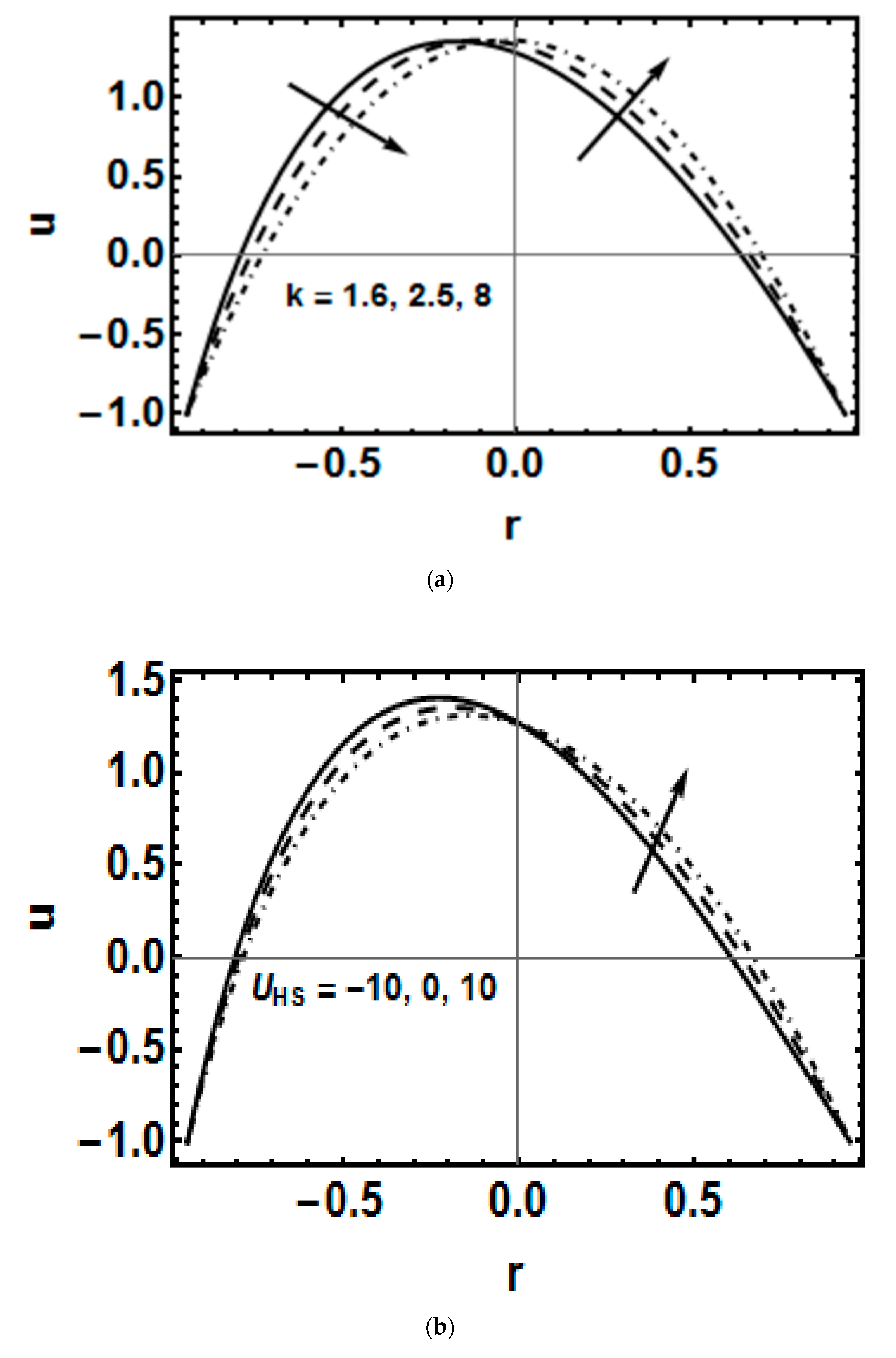
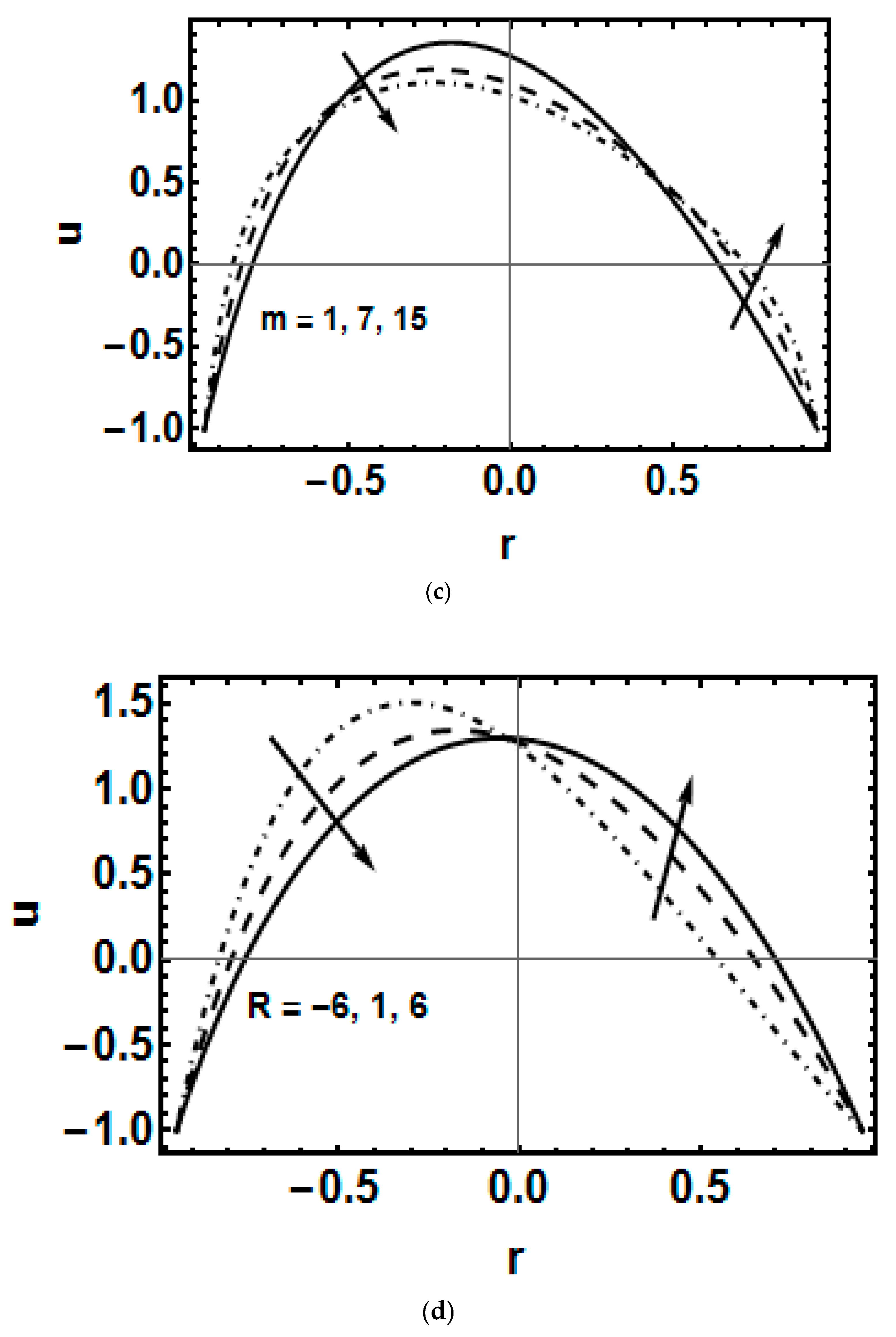
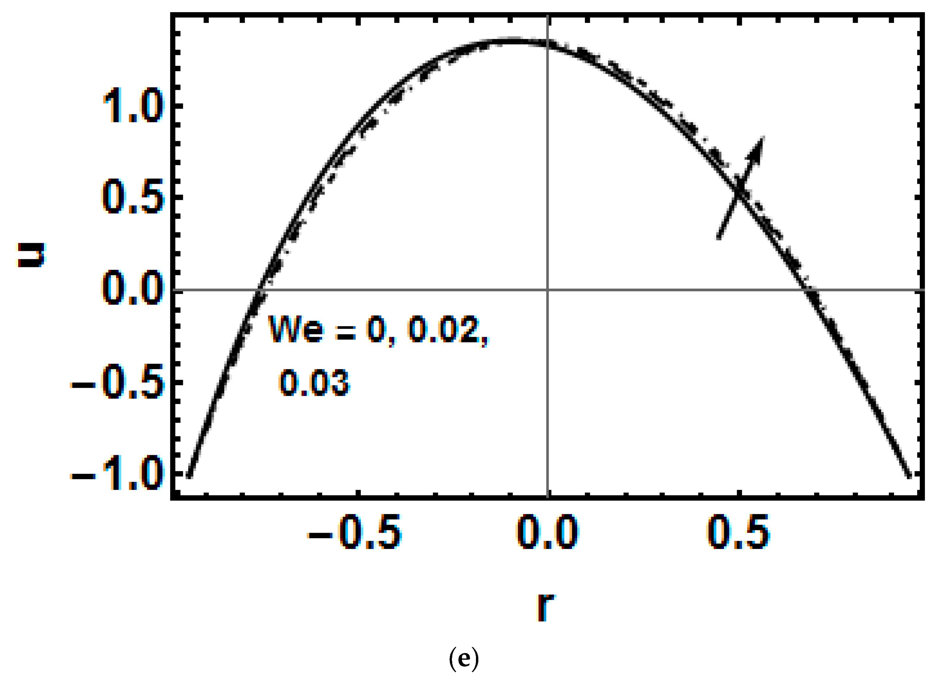
4. Results and Discussion

This section is devoted to discussing the impact of default values with the considered range for the non-dimensional numbers and parameters [33,34] such as electro-osmotic velocity $\left(U_{HS}\right)$, curvature $k$, electric double layer $\left(m\right)$ and zeta potential ratio $\left(R\right)$. Velocity graphs are shown with the variation in different parameters in Figure 2. In Figure 2a, the variation in the curvature’s effect on velocity is shown. This figure clearly shows that increasing $k$ causes velocity to decrease at the lower region of the wall, while velocity increases at the upper region of the wall. Moreover, for a straight channel, the velocity is symmetric about the central line. Figure 2b shows the variation in electro-osmotic velocity. When the direction of the electric field and flow are opposite, then velocity goes on increasing at the lower region of the wall; while, at the upper region of the wall, velocity decreases when the electric field and the motion of fluid are in the same direction. The values of electro-osmotic velocity are taken as −10, 0 and 10. Here, a positive number specifies that the electric field opposes the direction of the flow field, while a negative value shows that the electric field is in the same direction of flow field, while 0 represents the special case. The electric double layer thickness parameter is examined in Figure 2c. It is noticed that velocity goes on decreasing by changing the value of $m$ at the lower region of wall, while velocity increases at the upper region of wall. In Figure 2d, it is observed that velocity goes on decreasing by varying the values of the zeta potential ratio parameter at the lower region of wall, while velocity goes on increasing at the upper region of wall. If the zeta potential ratio is $R=1,$ then the potential of both walls is equal. When $r<0$, for a higher value of the zeta potential ratio parameter ranging from $R=-6,1,6$, velocity decreases and the converse result is observed for $r>0$. The effects of the Weissenberg number can be examined in Figure 2e. It is noted that velocity goes on decreasing by changing the value of the Weissenberg number at the lower region of wall, while velocity increases at the upper layer of wall.

Figure 3, shows the temperature effect in the curved micro-channel. From Figure 3a, we observed that temperature decreases when the value of curvature parameter is increased. The temperature has a major impact in the central region of the micro-channel. Therefore, temperature is controlled with the curvature in the central region. Figure 3b shows variation in electro-osmotic velocity. By raising the electro-osmotic velocity, temperature is reduced. Figure 3c explains the variation in $m$. The figure shows that raising the value of $m$ increases the temperature. An enhancement in the double layer thickness at the walls produce heating in the micro-channel. Figure 3d illustrates the $\left(R^{\prime }s\right)$ zeta potential. Temperature rises by increasing the zeta potential ratio $R$. The Weissenberg number can be observed in Figure 3e. Temperature enhances by increasing the value of the Weissenberg number. The Weissenberg number has a direct relationship with the relaxation time of the fluid which creates resistance to the fluid flow and, hence, the temperature rises. Figure 3f demonstrates the effect of the Brinkmann number $B_r$. By increasing the value of the Brinkmann number $B_r$, the transfer of heat which is formed by viscous dissipation becomes slower and this causes an increase in the temperature.

In peristaltic flow, trapping phenomenon occurs in which fluid behavior can be observed easily. Contour plots in physiological transportation for the stream lines have integral flow features which is known as trapping. Figure 4 deliberates the outcome of the curvature on stream lines. For the large values of curvature $k$, trapping bolus is large on the upper side of the micro-channel. In Figure 5, the electric double layer effect $m$ can be observed. The bolus moves in a downward direction and its size is also decreased. In addition, it has been noted that the diffusion of ions from the boundary to the diffusive layer is vital in trapping. In Figure 6, the electro-osmotic effect is observed. When the electric field and flow direction are the same $\left(U_{HS}=-9\right)$ the trapping stream lines are more, while when the electric field and flow direction are opposite $\left(U_{HS}=9\right)$ the trapping stream lines are less. The impact of the weissenberg number can be seen in Figure 7. The upper bolus moves towards the left while lower bolus become flatter.

Figure 8 is presented to portray the behavior of the Bejan number. In Figure 8a, $Be$ rises by increasing the value of the Brinkmann number. Br has a direct relationship with the square of the wave speed and viscosity, therefore, entropy increases. In Figure 8b, the variation in parameter $S$ can be examined. It is found that $Be$ declines by increasing the value of $S$. In Figure 8c, we can examine the variation in the Weissenberg number $We$. $Be$ increases by rising the value of the Weissenberg number. Figure 9 displays the consequence of different parameters on the total entropy production. In Figure 9a $,Ns$ grows by increasing the value of $B_r$. In Figure 9b, we observed the value of parameter $S$. It is observed from the figure that $Ns$ rises by increasing the value of $S$. In Figure 9c, we can examine the changes due to the variation in the Weissenberg number $We$. $Ns$ enhances by increasing the Weissenberg number. Figure 10 shows a good comparison with the previous finding.

5. Conclusions

In this article, peristaltic motion of Williamson fluid with electro-osmotic effect is illustrated. The heat equation is also modeled. Following this, key findings are observed:

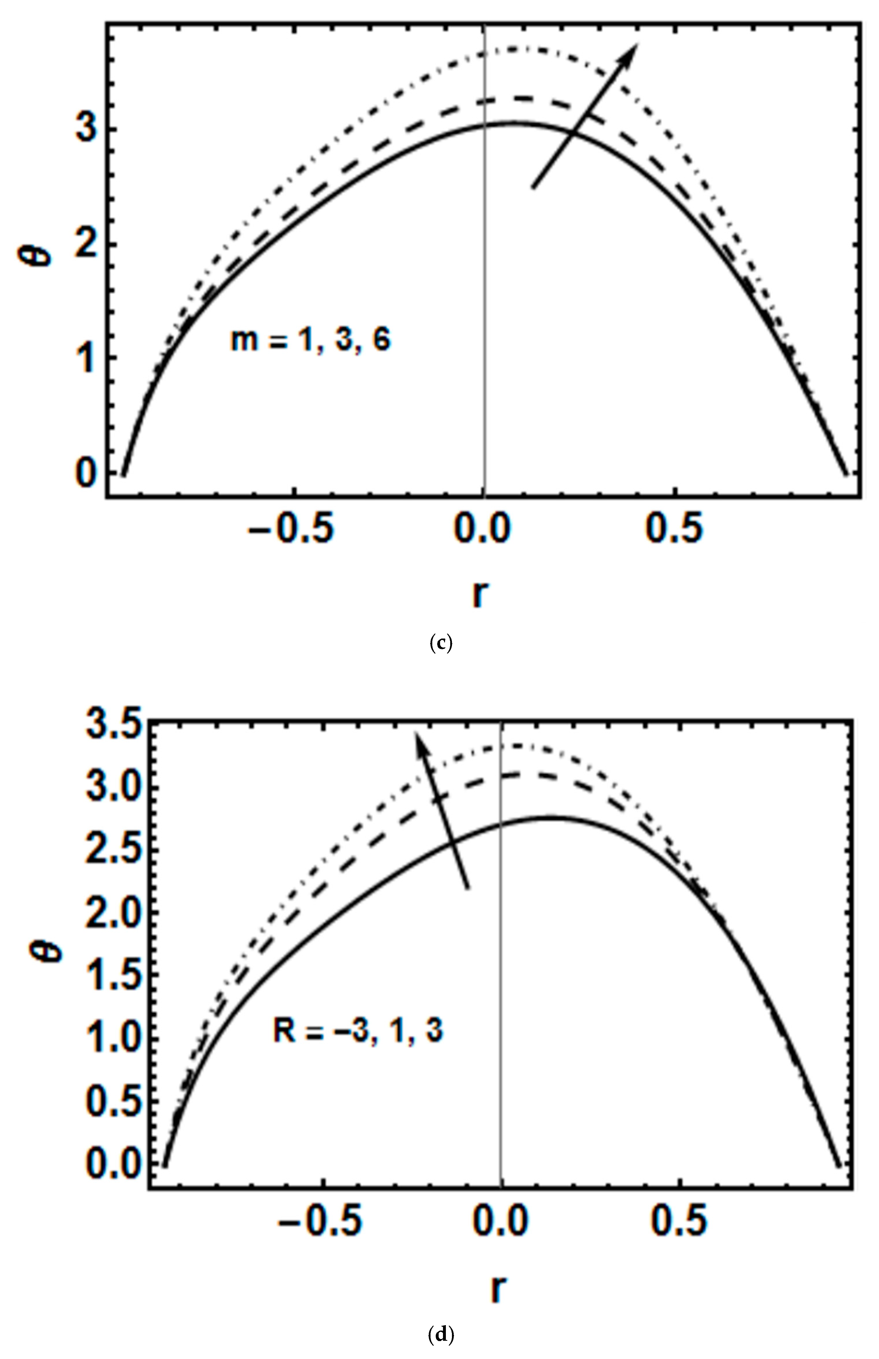
• The temperature rises for the thickness parameter.
• A rise in temperature is observed in the curved channel than the straight channel.
• Using the process of electro-osmosis, we can control the flow of fluid.
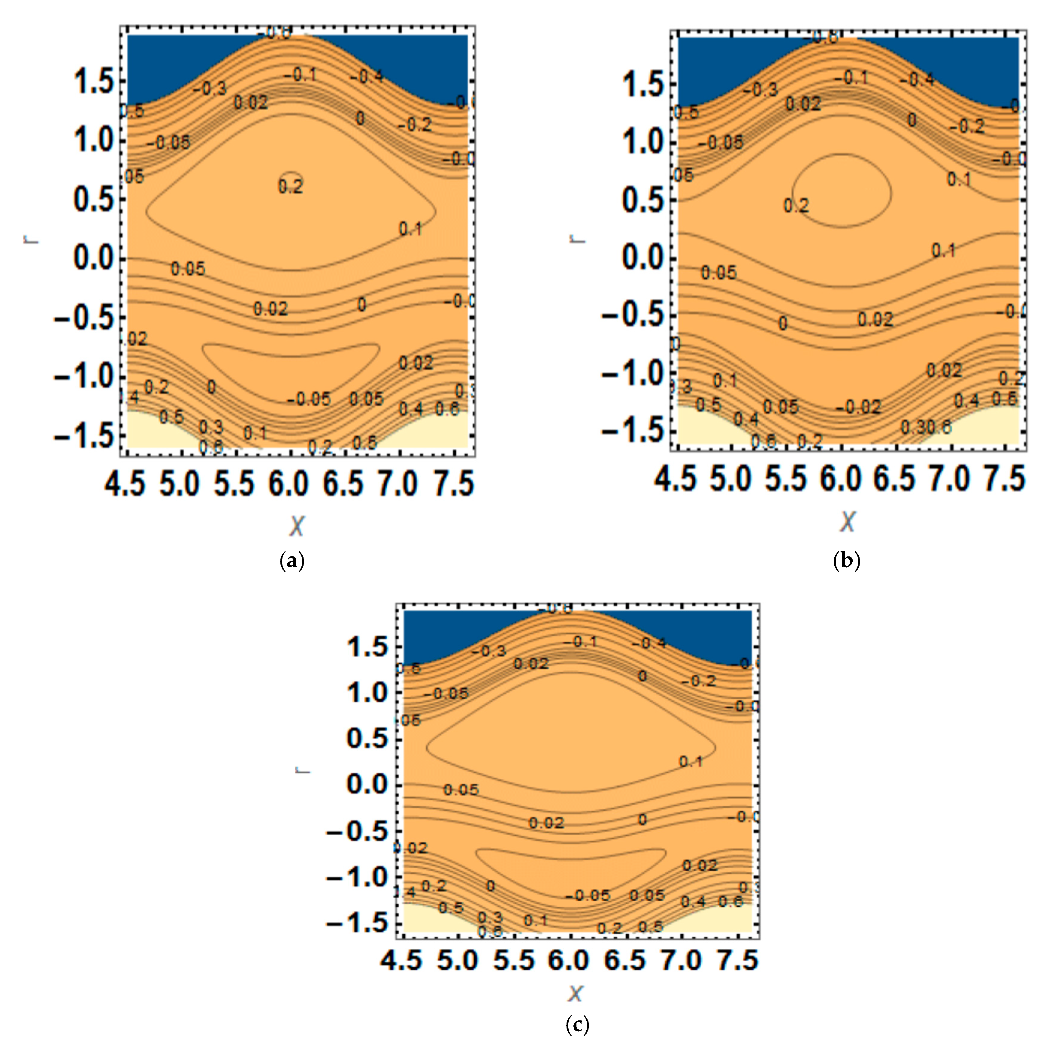
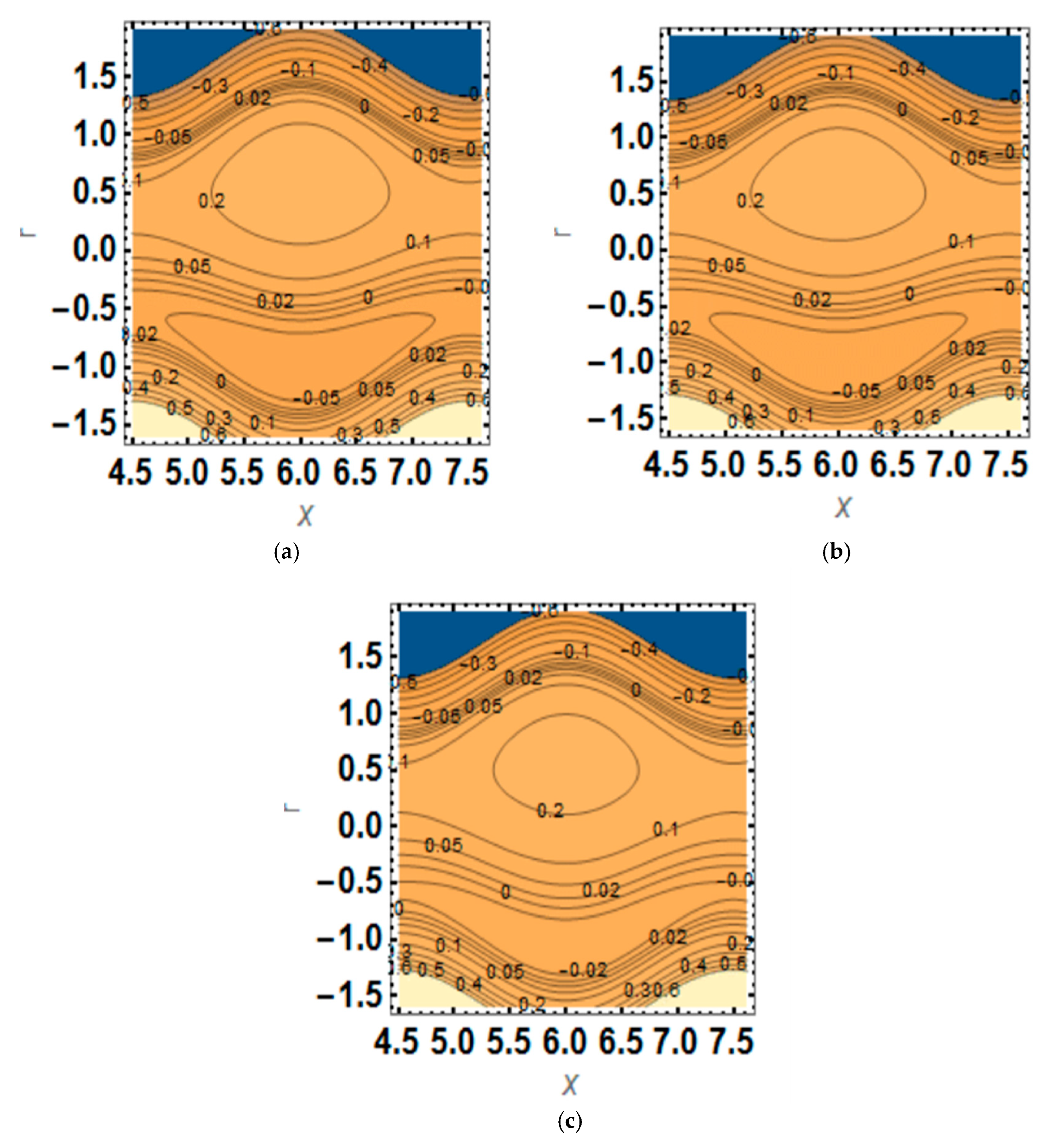
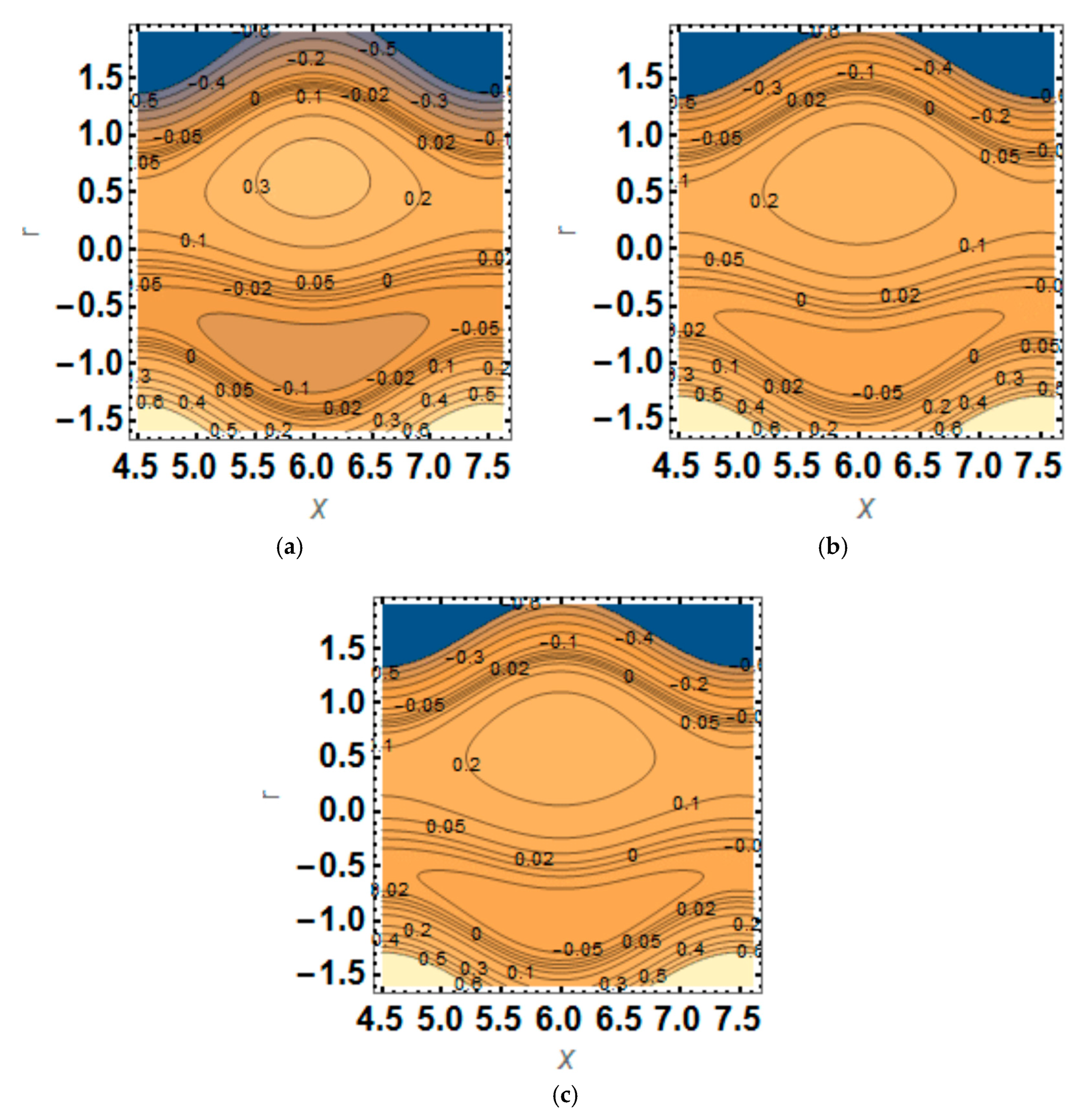
• The bolus size increases with the EDL thickness.
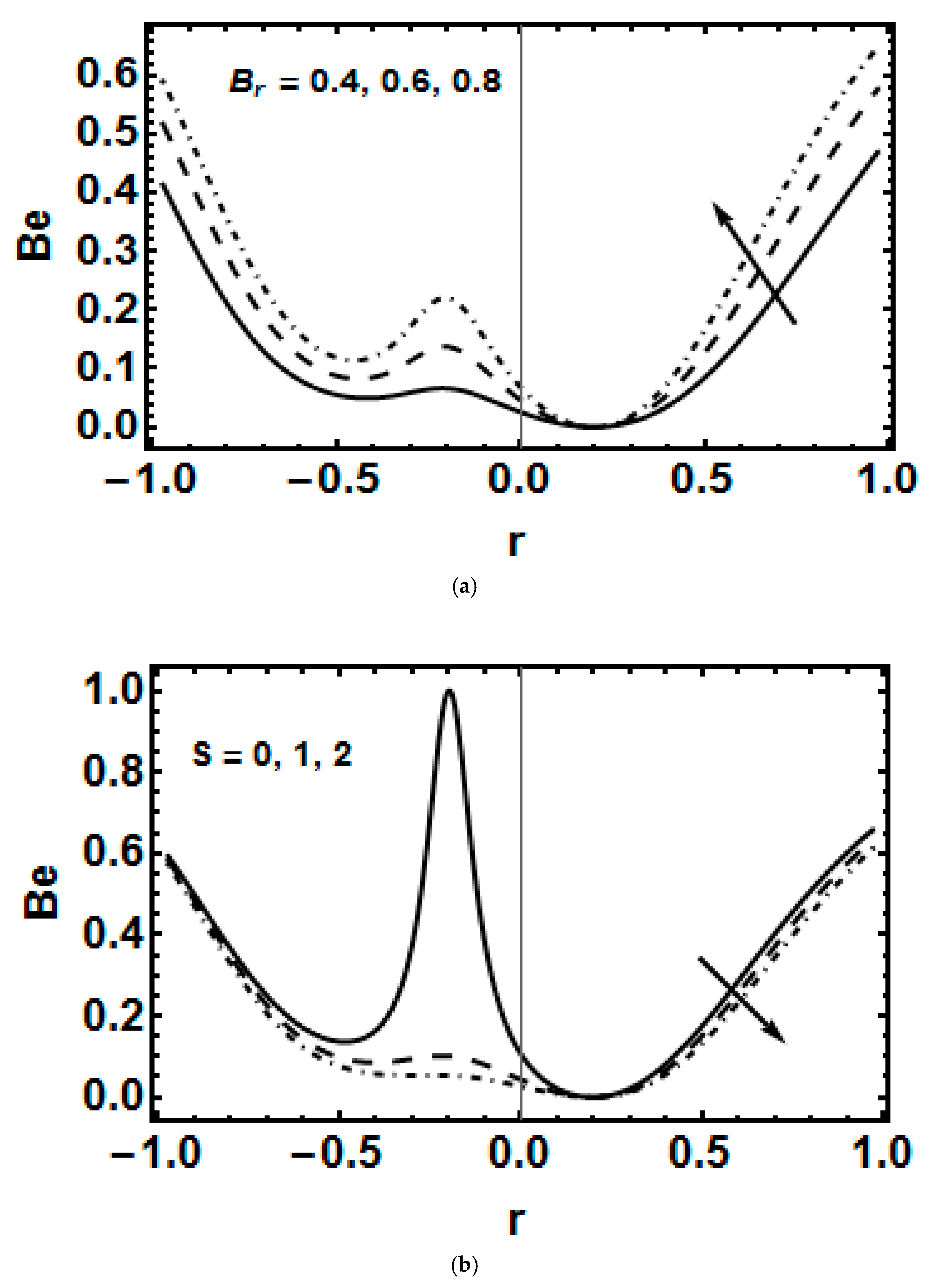
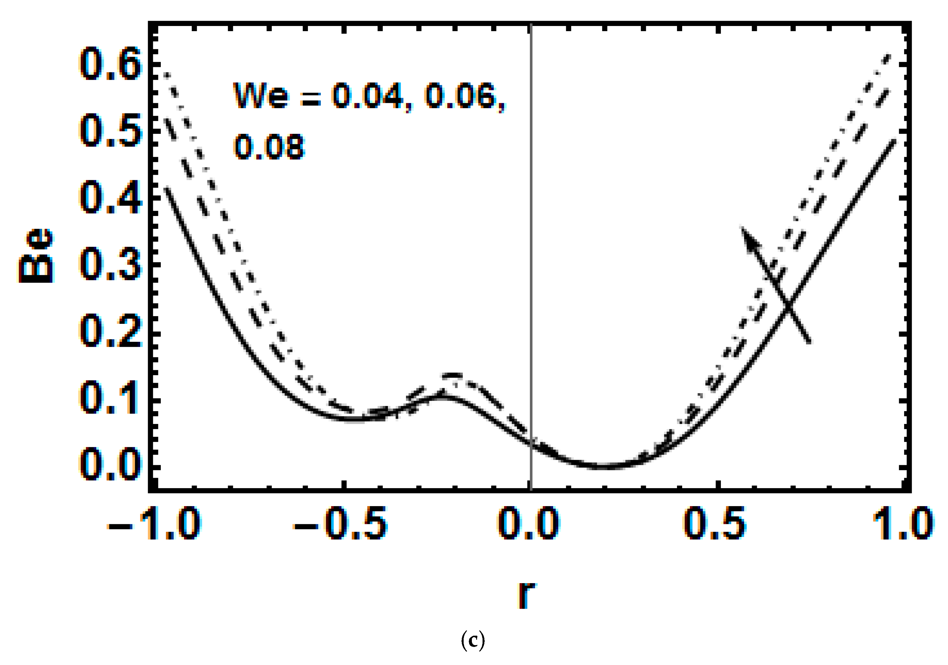
• The Bejan number enhances with both the Brickman number and the Weissenberg number.
• Using the process of electro-osmosis, the flow of fluid can be controlled easily.
• The current study has revealed some intriguing aspects of the curved micro-channel that are relevant to bio-microfluidic devices. Alternative rheological models, such as fourth grade fluid, may be considered in future studies.

References

1. Latham, T.W. Fluid Motions in a Peristaltic Pump. Master’s Thesis, Massachusetts Institute of Technology, Cambridge, MA, USA, 1966. [Google Scholar]
2. Jaffrin, M.Y.; Shapiro, A.H. Peristaltic pumping. Annu. Rev. Fluid Mech. 1971, 3, 13–37. [Google Scholar] [CrossRef]
3. Srivastava, L.M.; Srivastava, V.P. Peristaltic transport of blood: Casson model-II. J. Biomech. 1984, 17, 821–829. [Google Scholar] [CrossRef] [PubMed]
4. Raju, K.K.; Devanathan, R. Peristaltic motion of a non-Newtonian fluid. Rheol. Acta 1972, 11, 170–178. [Google Scholar] [CrossRef]
5. Sharifah, E.A.; Ali, I.; Muhammad, A.; Mazhar, A.; Weaam, A.; Haneen, H.; Awatif, A.; Asif, W. Thermal convection in nanofluids for peristaltic flow in a nonuniform channel. Sci. Rep. 2022, 12, 12656. [Google Scholar]
6. Nawaz, S.; Hayat, T.; Alsaedi, A. Analysis of entropy generation in peristalsis of Williamson fluid in curved channel under radial magnetic field. Comput. Methods Programs Biomed. 2019, 180, 105013. [Google Scholar] [CrossRef]
7. Vajravelu, K.; Sreenadh, S.; Rajanikanth, K.; Lee, C. Peristaltic transport of a Williamson fluid in asymmetric channels with permeable walls. Nonlinear Analysis: Real World Appl. 2012, 13, 2804–2822. [Google Scholar] [CrossRef]
8. Riaz, A.; Zeeshan, A.; Bhatti, M.M.; Ellahi, R. Peristaltic propulsion of Jeffrey nano-liquid and heat transfer through a symmetrical duct with moving walls in a porous medium. Phys. A Stat. Mech. Its Appl. 2020, 545, 123788. [Google Scholar] [CrossRef]
9. Chakraborty, S. Augmentation of peristaltic microflows through electro-osmotic mechanisms. J. Phys. D Appl. Phys. 2006, 39, 5356. [Google Scholar] [CrossRef]
10. Tripathi, D.; Sharma, A.; Bég, O.A. Electrothermal transport of nanofluids via peristaltic pumping in a finite micro-channel: Effects of Joule heating and Helmholtz-Smoluchowski velocity. Int. J. Heat Mass Transfer. 2017, 111, 138–149. [Google Scholar] [CrossRef]
11. Narla, V.K.; Tripathi, D.; Bég, O.A. Electro-osmotic nanofluid flow in a curved microchannel. Chin. J. Phys. 2020, 67, 544–558. [Google Scholar] [CrossRef]
12. Ambreen, A.K.; Kaenat, A.; Akbar, Z.; Anwar, B.; Tasveer, A.B. Electro-osmotic peristaltic flow and heat transfer in an ionic viscoelastic fluid through a curved micro-channel with viscous dissipation. Proc. Inst. Mech. Eng. Part H J. Eng. Med. 2022, 236, 1080–1092. [Google Scholar]
13. Ramesh, K.; Prakash, J. Thermal analysis for heat transfer enhancement in electroosmosis-modulated peristaltic transport of Sutterby nanofluids in a microfluidic vessel. J. Therm. Anal. Calorim. 2019, 138, 1311–1326. [Google Scholar] [CrossRef]
14. Akram, J.; Akbar, N.S.; Maraj, E.N. A comparative study on the role of nanoparticle dispersion in electroosmosis regulated peristaltic flow of water. Alex. Eng. J. 2020, 59, 943–956. [Google Scholar] [CrossRef]
15. Tripathi, D.; Yadav, A.; Bég, O.A. Electro-kinetically driven peristaltic transport of viscoelastic physiological fluids through a finite length capillary: Mathematical modeling. Math. Biosci. 2017, 283, 155–168. [Google Scholar] [CrossRef]
16. Tanveer, A.; Mahmood, S.; Hayat, T.; Alsaedi, A. On electroosmosis in peristaltic activity of MHD non-Newtonian fluid. Alexandria Eng. J. 2021, 60, 3369–3377. [Google Scholar] [CrossRef]
17. Bejan, A. Second law analysis in heat transfer. Energy 1980, 5, 720–732. [Google Scholar] [CrossRef]
18. Bejan, A. Entropy Generation Minimization: The Method of Thermodynamic Optimization of Finite-Size Systems and Finite Time Processes; CRC Press: Boca Raton, NY, USA, 2013; p. 23. [Google Scholar]
19. Jhorar, R.; Tripathi, D.; Bhatti, M.M.; Ellahi, R. Electro osmosis modulated biomechanical transport through asymmetric microfluidics channel. Indian J. Phys. 2018, 92, 1229–1238. [Google Scholar] [CrossRef]
20. Ellahi, R.; Sait, S.M.; Shehzad, N.; Mobin, N. Numerical simulation and mathematical modeling of electroosmotic Couette-Poiseuille flow of MHD power-law nanofluid with entropy generation. Symmetry 2019, 11, 1038. [Google Scholar] [CrossRef] [Green Version]
21. Bhatti, M.M.; Yousif, M.A.; Mishra, S.R.; Shahid, A. Simultaneous influence of thermo-diffusion and diffusion-thermo on non-Newtonian hyperbolic tangent magnetised nanofluid with Hall current through a nonlinear stretching surface. Pramana 2019, 93, 88. [Google Scholar] [CrossRef]
22. Gholamalipour, P.; Siavashi, M.; Doranehgard, M.H. Eccentricity effects of heat source inside a porous annulus on the natural convection heat transfer and entropy generation of Cu-water nanofluid. Int. Commun. Heat Mass Transfer. 2019, 109, 104367. [Google Scholar] [CrossRef]
23. Turkyilmazoglu, M. An analytical treatment for the exact solutions of MHD flow and heat over two–three dimensional deforming bodies. Int. J. Heat Mass Transfer. 2015, 90, 781–789. [Google Scholar] [CrossRef]
24. Zhang, L.; Bhatti, M.M.; Marin, M.; Mekheimer, K.S. Entropy analysis on the blood flow through anisotropically tapered arteries filled with magnetic zinc-oxide (ZnO) nanoparticles. Entropy 2020, 22, 1070. [Google Scholar] [CrossRef] [PubMed]
25. Banerjee, A.; Nayak, A.K. Influence of varying zeta potential on non-Newtonian flow mixing in a wavy patterned microchannel. J. Non-Newton. Fluid Mech. 2019, 269, 17–27. [Google Scholar] [CrossRef]
26. Rostamzadeh, A.; Razavi, S.E.; Mirsajedi, S.M. Towards multidimensional artificially characteristic-based scheme for incompressible thermo-fluid problems. Mechanics 2017, 23, 826–834. [Google Scholar] [CrossRef] [Green Version]
27. Trabzon, L.; Karimian, G.; RKhosroshahi, A.; Gül, B.; Gh Bakhshayesh, A.; Koçak, A.F.; Aldi, Y.E. High-throughput nanoscale liposome formation via electrohydrodynamic-based micromixer. Phys. Fluids 2022, 34, 102011. [Google Scholar] [CrossRef]
28. Sharma, B.K.; Kumar, A.; Gandhi, R.; Bhatti, M.M.; Mishra, N.K. Entropy Generation and Thermal Radiation Analysis of EMHD Jeffrey Nanofluid Flow: Applications in Solar Energy. Nanomaterials 2023, 13, 544. [Google Scholar] [CrossRef]
29. Gandhi, R.; Sharma, B.K.; Mishra, N.K.; Al-Mdallal, Q.M. Computer Simulations of EMHD Casson Nanofluid Flow of Blood through an Irregular Stenotic Permeable Artery: Application of Koo-Kleinstreuer-Li Correlations. Nanomaterials 2023, 13, 652. [Google Scholar] [CrossRef]
30. Sridhar, V.; Ramesh, K.; Gnaneswara Reddy, M.; Azese, M.N.; Abdelsalam, S.I. On the entropy optimization of hemodynamic peristaltic pumping of a nanofluid with geometry effects. Waves Random Complex Media 2022, 1–21. [Google Scholar] [CrossRef]
31. Narla, V.K.; Tripathi, D. Electroosmosis modulated transient blood flow in curved microvessels: Study of mathematical model. Microvasc. Res. 2019, 123, 25–34. [Google Scholar] [CrossRef]
32. Rashid, M.; Ansar, K.; Nadeem, S. Effects of induced magnetic field for peristaltic flow of Williamson fluid in a curved channel. Phys. A Stat. Mech. Its Appl. 2020, 553, 123979. [Google Scholar] [CrossRef]
33. Bhatti, M.M.; Riaz, A.; Zhang, L.; Sait, S.M.; Ellahi, R. Biologically inspired thermal transport on the rheology of Williamson hydromagnetic nanofluid flow with convection: An entropy analysis. J. Therm. Anal. Calorim. 2021, 144, 2187–2202. [Google Scholar] [CrossRef]
34. Ghorbani, G.; Moghadam, A.J.; Emamian, A.; Ellahi, R.; Sait, S.M. Numerical simulation of the electroosmotic flow of the Carreau-Yasuda model in the rectangular microchannel. Int. J. Numer. Methods Heat Fluid Flow 2022, 32, 2240–2259. [Google Scholar] [CrossRef]
Figure 1. Geometry of the problem.
Symmetry 15 00889 g001
Figure 2. (a): Shows variation in k on velocity field when m = 1 , W e = 0.01 , U H S = 1 and R = 0.5 . (b): Shows variation in U H S on velocity field when m = 1 , W e = 0.01 ,   R = 0.5   a n d   k = 1.5 . (c): Shows variation in electric double layer thickness m on velocity field when W e = 0.01 , U H S = 1 , R = 0.5 and k = 1.5 . (d): Shows variation in zeta potential R on velocity field when m = 1 , W e = 0.01 , U H S = 1  and  k = 1.5 . (e): Shows variation of W e on velocity field when m = 1 , U H S = 1 , R = 0.5   a n d   k = 1.5 .
Symmetry 15 00889 g002aSymmetry 15 00889 g002bSymmetry 15 00889 g002c
Figure 3. (a): Shows variation in k on temperature profile when m = 1 , W e = 0 , B r = 1 , U H S = 1 and R = 0.5 . (b): Shows variation in electro-osmotic force U H S on temperature profile when m = 1 , W e = 0 , B r = 1 , k = 1.5 and R = 0.5 . (c): Shows variation in electric double layer thickness m on temperature profile when k = 1.5 , W e = 0 , B r = 1 , U H S = 1 and R = 0.5 . (d): Shows variation in zeta potential R on temperature profile when m = 1 , W e = 0 , B r = 1 , U H S = 1 and k = 1.5 . (e): Shows variation in Weissenberg number W e on temperature profile when m = 1 , B r = 1 , k = 1.5 , U H S = 1 and R = 0.5 . (f): Shows variation in Brinkman number B r on temperature profile when m = 1 , W e = 0 , k = 1.5 , U H S = 1 and R = 0.5 .
Symmetry 15 00889 g003aSymmetry 15 00889 g003bSymmetry 15 00889 g003c
Figure 4. Stream lines for various values of curvature k when m = 3 ,   W e = 0.01 ,   U H S = 1   a n d   R = 0.5 . (a) ( k = 5 ) ; (b) ( k = 20 ) . (c) ( k = 30 ) .
Symmetry 15 00889 g004
Figure 5. Stream line for various value of m with k = 3 , R = 0.5 , W e = 0.01 and U H S = 1 . (a) m = 0.5 . (b) ( m = 1.1 ) . (c) ( m = 2.5 ) .
Symmetry 15 00889 g005
Figure 6. Stream line for various values of electroosmotic velocity U H S when k = 3   W e = 0.01 , m = 3   a n d   R = 0.5 . (a) ( U H S = 1 ) . (b) ( U H S = 0 ) . (c) ( U H S = 1 ) .
Symmetry 15 00889 g006
Figure 7. Stream line for various values of W e when k = 3 , R = 0.5 , U H S = 1 and m = 3 . (a) ( W e = 0.001 ) . (b) ( W e = 0.01 ) . (c) ( W e = 0.05 ) .
Symmetry 15 00889 g007
Figure 8. (a): Shows variation in B r on B e when m = 1 , k = 3 , U H S = 5 , R = 0.8 and W e = 0.06 . (b): Shows variation in S on B e when m = 1 , k = 3 , U H S = 5 , R = 0.8 and W e = 0.06 . (c): Shows variation in Weissenberg number W e on B e when m = 1 , k = 3 , U H S = 1 and R = 0.8 .
Symmetry 15 00889 g008aSymmetry 15 00889 g008b
Figure 9. (a): Shows variation in B r on N s when m = 1 , k = 3 , U H S = 5 , R = 0.8 and W e = 0.06 . (b): Shows variation of S on N s when m = 1 , k = 3 , U H S = 5 , R = 0.8 and W e = 0.08 . (c): Shows variation of Weissenberg number W e on N s when m = 1 , k = 3 , U H S = 5 and R = 0.8 .
Symmetry 15 00889 g009aSymmetry 15 00889 g009b
Figure 10. Comparison of velocity with Narla and Tripathi [31] and present work for k = 2 when W e = 0 .
Symmetry 15 00889 g010
Disclaimer/Publisher’s Note: The statements, opinions and data contained in all publications are solely those of the individual author(s) and contributor(s) and not of MDPI and/or the editor(s). MDPI and/or the editor(s) disclaim responsibility for any injury to people or property resulting from any ideas, methods, instructions or products referred to in the content.