Bounds for Extreme Zeros of Classical Orthogonal Polynomials Related to Birth and Death Processes

Abstract

In this paper, we consider birth and death processes with different sequences of transition rates and find the bound for the extreme zeros of orthogonal polynomials related to the three term recurrence relations and birth and death processes. Furthermore, we find the related chain sequences. Using these chain sequences, we find the transition probabilities for the corresponding process. As a consequence, transition probabilities related to G-fractions and modular forms are derived. Results obtained in this work are new and several graphical representations and numerical computations are provided to validate the results.

1. Introduction

Let us consider the second order differential equation

$$\sigma \left(x\right)y_n^{″}\left(x\right)+\tau \left(x\right)y_n^{\prime }\left(x\right)-{\lambda }_n{y}_n\left(x\right)=0,$$

(1)

where $\sigma \left(x\right)=a{x}^2+bx+c$ and $\tau \left(x\right)=dx+e$ are polynomials independent of n, ${\lambda }_n=n(n-1)a+nd$ is known as the eigenvalue parameter which depends on $n=0,1,2,\dots$ [1,2] and $a,b,c,d$ and e are real parameters. In the self-adjoint form of (1), the general weight function is given by

$$\begin{array}{c}\hfill W\left(x\right)=exp\left(\int \frac{dx+e}{a{x}^2+bx+c}dx\right).\end{array}$$

(2)

The parameters d and e in (2) depend on three independent parameters a, b and c. Consequently, we will have exactly six solutions of Equation (1) known as classical orthogonal polynomials (COPS). Classical orthogonal polynomials and Sturm–Liouville problems are also related to symmetry (see [3]). Classical orthogonal polynomials can also be characterized as finite COPS and infinite sequences. Jacobi, Leguerre and Hermite orthogonal polynomials are three well-known cases of infinite orthogonal sequences while the other three finite COPS are less familiar in the literature. In [4], Masjed-Jamei characterized the finite cases and studied various properties. For details of this literature we refer to [4,5,6,7] and references cited therein. In [4], these finite COPS are categorized as first, second and third classes, based on their connection with Jacobi, Hermite and Bessel functions, respectively. The R-Jacobi, R-Hermite, and R-Bessel polynomials can also be used to represent these classes of polynomials. Here, R- stands for Routh or Romonovski, because Routh [8] and Romonovski [9] introduced and studied these classes independently. For further details regarding this literature can be found in [5,6,9] and references cited therein. In [5,6], Malik and Swaminathan called these R-Jacobi, R-Hermite and R-Bessel finite COPS as Type I, Type II and Type III COPS, respectively. The following Table 1 gives details of all the six classical orthogonal polynomials.

Table 1. Characteristics of classical orthogonal polynomials.

Type	Polynomial	$\mathit{\sigma }\left(\mathit{x}\right)$	$\mathit{\tau }\left(\mathit{x}\right)$	Weight Function	Interval
	Jacobi	$1-x^2$	$-(\alpha +\beta +2)x+(\beta -\alpha )$	${(1-x)}^{\alpha }{(1+x)}^{\beta }\alpha ,\beta >-1$	$[-1,1]$
Infinite	Laguerre	x	$\alpha +1-x$	$x^{\alpha }exp(-x);\alpha >-1$	$[0,\infty )$
	Hermite	1	$-2x$	$exp\left(x^2\right)$	$(-\infty ,\infty )$
	R-Jacobi	$x^2+x$	$(2-p)x+(1+q)$	$x^q{(1+x)}^{-(p+q)}$	$[0,\infty )$
Finite	R-Hermite	$x^2+1$	$(3-2p)x$	${(1+x^2)}^{-(p-1/2)}$	$(-\infty ,\infty )$
	R-Bessel	$x^2$	$(2-p)x+1$	$x^{-p}exp(-1/x)$	$[0,\infty )$

Let ${\left\{p_n\right\}}_{n=0}^{\infty }$ be a sequence of classical orthogonal polynomials. Then it satisfies the following three term recurrence relation

$$\begin{array}{cc}\hfill x{p}_n\left(x\right)& ={\alpha }_n{p}_{n+1}\left(x\right)+{\beta }_n{p}_n\left(x\right)+{\gamma }_n{p}_{n-1}\left(x\right),\hfill \\ \hfill p_0\left(x\right)& =1,p_1\left(x\right)=(x-{\beta }_0)/{\alpha }_0.\hfill \end{array}$$

(3)

with ${\alpha }_{n-1}{\gamma }_n>0$ for $0<n<N$. COPS have lot of applications in mathematical biology, queueing theory and other fields of pure and applied mathematics. In this paper, we consider the applications of COPS, especially R-Jacobi and R-Bessel polynomials in birth and death processes. Before proceeding towards the main results, let us provide a short introduction about birth and death processes.

A special case of the continuous time Markov process is the birth and death process whose transition probabilities are defined as

$$\begin{array}{c}\hfill p_{m,n}\left(t\right)=\mathbf{Pr}\{X\left(t\right)=n|X\left(0\right)=m\}\end{array}$$

(4)

and states are labelled by non-negative integers.

Let ${\lambda }_m$ and ${\mu }_m$ be birth and death rates, respectively, for $m=0,1,2,\dots$ and ${\mu }_0\ge 0$. Then the transition probabilities $p_{m,n}\left(t\right)$ satisfy the following

$$\begin{array}{c}\hfill p_{m,n}\left(t\right)=\left\{\begin{array}{cc}{\lambda }_{i}t+o\left(t\right),\hfill & \mathrm{if}n=m+1;\hfill \\ {\mu }_{i}t+o\left(t\right),\hfill & \mathrm{if}n=m-1;\hfill \\ 1-t({\lambda }_i+{\mu }_i)+o\left(t\right),\hfill & \mathrm{if}n=m;\hfill \\ o\left(t\right),\hfill & \mathrm{otherwise}.\hfill \end{array}\right.\end{array}$$

Theorem 1

([10] Theorem 5.2.1). Transition probabilities $\{p_{m,n}\left(t\right):m,n=0,1,\dots \}$ satisfy the following Chapman–Kolmogorov differential equations

$$\begin{array}{cc}\hfill {\displaystyle \frac{d}{dt}}{p}_{m,n}\left(t\right)& ={\lambda }_{n-1}{p}_{m,n-1}+{\mu }_{n+1}{p}_{m,n+1}-({\lambda }_n+{\mu }_n)p_{m,n}\left(t\right),\hfill \end{array}$$

(5)

$$\begin{array}{cc}\hfill {\displaystyle \frac{d}{dt}}{p}_{m,n}\left(t\right)& ={\lambda }_m{p}_{m+1,n}+{\mu }_m{p}_{m-1,n}-({\lambda }_n+{\mu }_n)p_{m,n}\left(t\right).\hfill \end{array}$$

(6)

It is well known that birth and death processes and orthogonal polynomials are related to each other [10,11].

Let

$$p_{m,n}\left(t\right)=f\left(t\right)Q_m{F}_n.$$

Then, from Theorem 1, we have [10] (p. 137)

$$\begin{array}{cc}\hfill -x{F}_n\left(x\right)& ={\lambda }_{n-1}{F}_{n-1}\left(x\right)+{\mu }_{n+1}{F}_{n+1}\left(x\right)-({\lambda }_n+{\mu }_n)F_n\left(x\right),n>0\hfill \\ \hfill F_{-1}\left(x\right)& =0,F_0\left(x\right)=1\hfill \end{array}$$

(7)

and

$$\begin{array}{cc}\hfill -x{Q}_n\left(x\right)& ={\lambda }_n{Q}_{n+1}\left(x\right)+{\mu }_n{Q}_{n-1}\left(x\right)-({\lambda }_n+{\mu }_n)Q_n\left(x\right),n>0\hfill \\ \hfill Q_0\left(x\right)& =1,Q_{-1}\left(x\right)=0\hfill \end{array}$$

(8)

The family of polynomials $\left\{Q_n\left(x\right)\right\}$ are called birth and death polynomials.

The following theorem describes the behaviour of zeros of birth and death process polynomials.

Theorem 2

([10] Theorem 7.2.5). The zeros of birth and death process polynomials belong to $(0,\infty )$.

In this paper, our objective is to find the bounds for the extreme zeros of the finite classes of orthogonal polynomials related to birth and death processes with the help of chain sequences.

Definition 1

(Chain Sequences [12]). A sequence ${\left\{a_n\right\}}_{n=1}^{\infty }$ is called a chain sequence if there exists a sequence ${\left\{g_k\right\}}_{k=0}^{\infty }$ such that

(i)

$0\le g_0<1,0<g_n<1,n\ge 1$

(ii)

$a_n=(1-g_{n-1})g_n,n=1,2,3,\dots$,

where the sequence $\left\{g_k\right\}$ is known as the parameter sequence for $\left\{a_n\right\}$.

Let us recall the following well-known results, which will be useful to prove the main results of this manuscript.

Lemma 1

([13]). The chain sequences associated with (3) and birth and death processes with transition rates ${\lambda }_n$ and ${\mu }_n$ for $m,n=0,1,\dots$ are given by

$$\begin{array}{c}\hfill {\displaystyle \frac{{\alpha }_{n-1}{\gamma }_n}{{\beta }_n{\beta }_{n-1}}}={\displaystyle \frac{{\mu }_n}{{\lambda }_n+{\mu }_n}}\left(1-{\displaystyle \frac{{\mu }_{n-1}}{{\lambda }_{n-1}+{\mu }_{n-1}}}\right).\end{array}$$

(9)

Theorem 3

([13] Theorem 2). Let ${\left\{a_n\right\}}_{n=1}^{N-1}$ be a chain sequence and

$$\begin{array}{c}\hfill B:=max\{x_n:0<n<N\}\mathrm{and}A:=min\{y_n:0<n<N\},\end{array}$$

(10)

where $x_n$ and $y_n$, $x_n>y_n$ are the roots of the equation

$$\begin{array}{c}\hfill (x-{\beta }_n)(x-{\beta }_{n-1})a_n={\gamma }_n{\alpha }_{n-1};\end{array}$$

(11)

i.e.,

$$\begin{array}{c}\hfill x_n,y_n={\displaystyle \frac{1}{2}}({\beta }_n+{\beta }_{n-1})\pm {\displaystyle \frac{1}{2}}\sqrt{{({\beta }_n-{\beta }_{n-1})}^2+4{\gamma }_n{\alpha }_{n-1}/a_n}.\end{array}$$

(12)

Then the zeros of $p_N\left(x\right)$ lie in $(A,B)$.

In 1924, G. U. Yule [14] considered the simplest model of birth and death processes. In [15], quartic transition rates of birth and death processes have been studied. Recently, new Nevanlinna matrices for orthogonal polynomials related to cubic birth and death processes have been derived in [16]. In [13], bounds for extreme zeros of Laguerre, associated Laguerre, Meixner, and MeixnerPollaczek polynomials have been found by M. E. H. Ismail and X. Li. These polynomials are also related to birth and death processes. The above results motivate us to consider R-Jacobi and R-Bessel polynomials and relate them with the birth and death processes and derive the bounds for extreme zeros of these polynomials.

2. R-Jacobi Polynomials Related to Birth and Death Processes

R-Jacobi polynomials are defined as follows ([4], Equation (2.2)):

$$\begin{array}{c}\hfill M_n^{(p,q)}\left(x\right)={(-1)}^{n}n!\sum _{k=0}^n\left(\genfrac{}{}{0pt}{}{p-(n+1)}{k}\right)\left(\genfrac{}{}{0pt}{}{q+n}{n-k}\right){(-x)}^k,\end{array}$$

(13)

where $\left(\genfrac{}{}{0pt}{}{n}{k}\right)={\displaystyle \frac{n!}{k!(n-k)!}}$ and $p>\{2maxn+1\},q>-1$.

The polynomials $M_n^{(p,q)}\left(x\right)$ satisfy the following differential Equation ([4], Equation (2.1))

$$\begin{array}{c}\hfill x(1+x)y^{″}\left(x\right)+\{(2-p)x+(1+q)\}{y}^{\prime }\left(x\right)-n(n+1-p)y\left(x\right)=0.\end{array}$$

(14)

The orthogonality relation for these polynomials is given in the following theorem.

Theorem 4

([4] Corollary 2).

$$\begin{array}{c}\hfill {\int }_0^{\infty }{\displaystyle \frac{x^q}{{(1+x)}^{p+q}}}{M}_n^{(p,q)}\left(x\right)M_m^{(p,q)}\left(x\right)=\left({\displaystyle \frac{n!(p-(n+1\left)\right)!(q+n)!}{(p-(2n+1\left)\right)(p+q-(n+1\left)\right)!}}\right){\delta }_{n,m}\end{array}$$

if and only if: $m,n=0,1,2,\dots ,N<(p-1)/2,q>-1,$ and

$${\delta }_{m,n}=\left\{\begin{array}{cc}0,\hfill & n\ne m,\hfill \\ 1,\hfill & n=m.\hfill \end{array}\right.$$

These polynomials can also be expressed [4] in terms of hypergeometric function [17] as follows:

$$\begin{array}{c}\hfill M_n^{(p,q)}\left(x\right)={(-1)}^{n}n!\left(\genfrac{}{}{0pt}{}{q+n}{n}\right){(x+1)}^n{}_2{F}_1\left(-n,p+q-n,q+1;{\displaystyle \frac{x}{x+1}}\right),\end{array}$$

where ${\displaystyle {}_2{F}_1(a,b;c;x)=1+\sum _{k=1}^{\infty }\frac{{\left(a\right)}_k{\left(b\right)}_k{x}^k}{{\left(c\right)}_{k}k!}}$ denotes hypergeometric function [17], with the notation ${\left(\alpha \right)}_k$, defined as

$$\begin{array}{cc}\hfill {\left(\alpha \right)}_k& =\alpha (\alpha +1)\cdots (\alpha +k-1)fork\ge 1,\hfill \\ \hfill {\left(\alpha \right)}_0& =1,\alpha \ne 0.\hfill \end{array}$$

(15)

Theorem 5.

Let $L(n,p,q)$ and $S(n,p,q)$ be the largest and smallest zeros of R-Jacobi polynomials $M_n^{(p,q)}\left(x\right)$. Then

$$\begin{array}{c}\hfill A<S(n,p,q)<L(n,p,q)<B\end{array}$$

(16)

where

$$\begin{array}{cc}\hfill A& =\frac{p(q+2n)-2(n^2-1)}{p(p-4n)+4(n^2-1)}-\frac{1}{(p-2n)}\sqrt{\frac{4n(-n+p)(n+q)(-n+p+q)}{(-1-2n+p)(1-2n+p)}+\frac{p^2{(p+2q)}^2}{{(-4+4n^2-4np+p^2)}^2}}\hfill \\ \hfill B& =\frac{p(q+2n)-2(n^2-1)}{p(p-4n)+4(n^2-1)}+\frac{1}{(p-2n)}\sqrt{\frac{4n(-n+p)(n+q)(-n+p+q)}{(-1-2n+p)(1-2n+p)}+\frac{p^2{(p+2q)}^2}{{(-4+4n^2-4np+p^2)}^2}}\hfill \end{array}$$

Proof. 

First, we consider the following three term recurrence relation ([4], Equation (2.19)) of R-Jacobi polynomials:

$$\begin{array}{cc}\hfill M_{n+1}^{(p,q)}\left(x\right)& =\left({\displaystyle \frac{(p-(2n+1\left)\right)(p-(2n+2\left)\right)}{(p-(n+1\left)\right)}}x\right.\hfill \\ \hfill & +\left.{\displaystyle \frac{(p-(2n+1\left)\right)\left(2n\right(n+1)-p(q+2n+1\left)\right)}{(p-(n+1\left)\right)(p-2n)}}\right)M_n^{(p,q)}\left(x\right)\hfill \\ \hfill & -\left({\displaystyle \frac{n(p-(2n+2\left)\right)(p+q-n)(q+n)}{(p-(n+1\left)\right)(p-2n)}}\right)M_{n-1}^{(p,q)}\left(x\right).\hfill \end{array}$$

(17)

Using (8) and (17), it can be easily shown that R-Jacobi polynomials are related to birth and death processes with transition rates

$$\begin{array}{c}\hfill \frac{(q+n)(p-n)}{(p-2n)(p-2n+1)}\mathrm{and}\frac{(n-1)(p+q-n+1)}{(p-2n+1)(p-2n+2)}\mathrm{for}n\ge 1.\end{array}$$

Using Lemma 1, we obtain the chain sequence related to R-Jacobi polynomials as follows:

$$\begin{array}{c}\hfill \frac{{\alpha }_{n-1}{\gamma }_n}{{\beta }_n{\beta }_{n-1}}=\frac{n(p+q-n)(p-2n-2)}{(p-2n-1)\left\{p\right(q+2n+1)-2n(n+1\left)\right\}}\left[1-\frac{(n-1)(p+q-n+1)(p-2n)}{(p-2n+1)\left\{p\right(q+2n-1)-2n(n-1\left)\right\}}\right].\end{array}$$

Finally, using Theorem 3 with the condition $a_n=\frac{1}{4}$ and recurrence relation (17), we obtain the required result. □

The inequality (16) is validated numerically in the following Table 2 for different values of p, q and n.

Table 2. Upper and lower bounds for different values of p, q and n.

Value of p, q, n	A	S(n, p, q)	L(n, p, q)	B
p = 30, q = 1, n = 5	0.000848214	0.025003868	0.182868373	0.677473464
p = 100, q = 3, n = 5	0.003256378	0.015689532	0.052264761	0.306032160
p = 50, q = 5, n = 10	0.013386412	0.036491151	0.399137716	2.334827874
p = 150, q = 10, n = 20	0.0075034407	0.015606200	0.235232011	1.100631480

3. R-Bessel Polynomials Related to Birth and Death Processes

R-Bessel polynomials are defined as [4]

$$\begin{array}{c}\hfill N_n^{\left(p\right)}\left(x\right)={(-1)}^n\sum _{k=0}^{n}k!\left(\genfrac{}{}{0pt}{}{p-(n+1)}{k}\right)\left(\genfrac{}{}{0pt}{}{n}{n-k}\right){(-x)}^k.\end{array}$$

(18)

These polynomials are solutions of the following differential equation

$$\begin{array}{c}\hfill x^2{y}^{″}\left(x\right)+\{(2-p)x+1\}{y}^{\prime }\left(x\right)-n(n+1-p)y\left(x\right)=0.\end{array}$$

(19)

The orthogonality relation for these polynomials is given in the following theorem:

Theorem 6

([4]). R-Bessel polynomials satisfy the following orthogonality relation:

$$\begin{array}{c}\hfill {\int }_0^{\infty }{x}^{-p}{e}^{-1/x}{N}_n^{\left(p\right)}\left(x\right)N_m^{\left(p\right)}\left(x\right)dx=\left({\displaystyle \frac{n!(p-(n+1\left)\right)!}{p-(2n+1)}}\right){\delta }_{n,m}\iff m,n=0,1,2,\dots ,N<\frac{p-1}{2}.\end{array}$$

These polynomials can also be expressed [4] in terms of hypergeometric functions [17] as follows:

$$\begin{array}{c}\hfill N_n^{\left(p\right)}\left(x\right)=n!\left(\genfrac{}{}{0pt}{}{p-1-n}{n}\right)x^n{}_1{F}_1\left(-n,p-2n;{\displaystyle \frac{1}{x}}\right).\end{array}$$

Here, ${\displaystyle {}_1{F}_1(a;b;x)=1+\sum _{k=1}^{\infty }\frac{{\left(a\right)}_k{x}^k}{{\left(b\right)}_{k}k!}}$ is known as hypergeometric function [17], where the notation ${\left(\alpha \right)}_k$ is defined in (13).

Theorem 7.

Let $L(n,p)$ and $S(n,p)$ be the largest and smallest zeros of R-Bessel polynomials $N_n^p\left(x\right)$. Then

$$\begin{array}{c}\hfill A<S(n,p)<L(n,p)<B\end{array}$$

(20)

where

$$\begin{array}{cc}\hfill A& =\frac{p}{p(p-4n)+4(n^2-1)}+\frac{2}{(p-2n)}\sqrt{\frac{n(p-n)}{(p-2n-1)(p-2n+1)}+\frac{p^2}{{(p^2-4np+4n^2-4)}^2}}\hfill \\ \hfill B& =\frac{p}{p(p-4n)+4(n^2-1)}-\frac{2}{(p-2n)}\sqrt{\frac{n(p-n)}{(p-2n-1)(p-2n+1)}+\frac{p^2}{{(p^2-4np+4n^2-4)}^2}}\hfill \end{array}$$

Proof. 

It is well-known that R-Bessel polynomials satisfy the following three term recurrence relation ([4], Equation (4.19)):

$$\begin{array}{cc}\hfill N_{n+1}^{\left(p\right)}\left(x\right)& =\left({\displaystyle \frac{(p-(2n+2\left)\right)(p-(2n+1\left)\right)}{p-(n+1)}}x-{\displaystyle \frac{p(p-(2n+1\left)\right)}{(p-(n+1\left)\right)(p-2n)}}\right)N_n^{\left(p\right)}\left(x\right)\hfill \\ \hfill & -{\displaystyle \frac{n(p-(2n+2\left)\right)}{(p-(n+1\left)\right)(p-2n)}}{N}_{n-1}^{\left(p\right)}\left(x\right).\hfill \end{array}$$

(21)

With the help of (8) and (21), it can be shown that R-Bessel polynomials are related to birth and death processes with transition rates

$$\begin{array}{c}\hfill \frac{(p-n-1)}{(p-2n-1)(p-2n-2)}\mathrm{and}\frac{n}{(p-2n-1)(p-2n)},\mathrm{for}n\ge 1.\end{array}$$

The chain sequence related to R-Bessel polynomials is given by

$$\begin{array}{c}\hfill {\displaystyle \frac{{\alpha }_{n-1}{\gamma }_n}{{\beta }_n{\beta }_{n-1}}}=\frac{n(p-2n-2)}{p(p-2n-1)}\left[1-\frac{(n-1)(p-2n)}{p(p-2n+1)}\right].\end{array}$$

Finally, using Theorem 3 with the condition $a_n=\frac{1}{4}$ and recurrence relation (21), the required result can be obtained. □

The inequality (20) is validated numerically in the following Table 3 for different values of p and n.

Table 3. Upper and lower bounds for different values of p and n.

Values of p, n	A	S(n,p)	L(n,p)	B
p = 60, n = 25	0.0174143242	0.001100195	0.127635714	1.232585676
p = 50, n = 20	0.0175690519	0.001590043	0.108368111	1.024097615
p = 70, n = 30	0.0177484733	0.000807141	0.146851849	1.440584860
p = 90, n = 40	0.0192205990	0.000489853	0.185209710	1.855779401

4. Birth and Death Processes with Different Sequences of Transition Rates

In this section, we will derive bounds for the smallest and largest zeros of birth and death process polynomials.

Theorem 8.

Let $L\left(n\right)$ and $S\left(n\right)$ be the largest and smallest zeros of birth and death process polynomials with transition rates ${\lambda }_n$ and ${\mu }_n$. Then

$$\begin{array}{c}\hfill A<S\left(n\right)<L\left(n\right)<B\end{array}$$

(22)

where

$$\begin{array}{ccc}\hfill A& =& {\displaystyle \frac{1}{2}}[({\lambda }_n+{\lambda }_{n-1})+({\mu }_n+{\mu }_{n-1})]-\sqrt{{\displaystyle \frac{1}{4}}{\{({\lambda }_n-{\lambda }_{n-1})+({\mu }_n-{\mu }_{n-1})\}}^2+4{\lambda }_{n-1}{\mu }_n},\hfill \\ \hfill B& =& {\displaystyle \frac{1}{2}}[({\lambda }_n+{\lambda }_{n-1})+({\mu }_n+{\mu }_{n-1})]+\sqrt{{\displaystyle \frac{1}{4}}{\{({\lambda }_n-{\lambda }_{n-1})+({\mu }_n-{\mu }_{n-1})\}}^2+4{\lambda }_{n-1}{\mu }_n}.\hfill \end{array}$$

Proof. 

Setting $Q_n\left(x\right)=p_n\left(x\right)$ and comparing (8) and (3), we obtain

$$\begin{array}{cc}\hfill {\alpha }_n& =-{\lambda }_n,{\gamma }_n=-{\mu }_n,\hfill \\ \hfill {\beta }_n& ={\lambda }_n+{\mu }_n.\hfill \end{array}$$

Now, we will use Theorem 3 to complete the proof. Putting the above values of ${\alpha }_{,}{\beta }_n$ and ${\gamma }_n$ in (12) with $a_n=\frac{1}{4}$, the required result can be established. □

Example 1

(Cubic Rates). Let us consider birth and death processes with cubic transition rates as in [16]:

$$\begin{array}{c}\hfill {\lambda }_n={(3n+1)}^2(3n+2),{\mu }_n=(3n-1){\left(3n\right)}^2.\end{array}$$

(23)

We have computed upper and lower bounds in the following Table 4 for $n=1,2,3,4,5$.

Table 4. Upper and lower bounds for cubic rates for $n=1,2,3,4,5$.

Value of n	B	A
n = 1	99.47726751	0.52273249
n = 2	672.2966054	−2.2966054
n = 3	2326.965295	−6.965295
n = 4	5709.384764	−11.384764
n = 5	11467.58306	−15.583056

Example 2

(Quartic Rates). We consider quartic transition rates as in [15]:

$$\begin{array}{c}\hfill {\lambda }_n=(4n+1){(4n+2)}^2(4n+3),{\mu }_n=(4n-1){\left(4n\right)}^2(4n+1).\end{array}$$

(24)

We have computed upper and lower bounds in the following Table 5 for $n=1,2,3$.

Table 5. Upper and lower bounds for quartic rates for $n=1,2,3$.

Value of n	B	A
n = 1	1294.470417	1.5295830
n = 2	14248.78880	−16.788798
n = 3	69140.94425	−116.94425

5. Birth and Death Processes Related to g-Fraction

In this section, we consider a special type of birth and death process with rates satisfying the condition

$$\begin{array}{c}\hfill {\lambda }_n+{\mu }_n=1,n=1,2,\dots \end{array}$$

(25)

with ${\mu }_0=0,{\lambda }_0=1$. Clearly, ${\alpha }_n={\lambda }_{n-1}{\mu }_n=(1-{\mu }_{n-1}){\mu }_n$ is a chain sequence.

Applying Laplace transform of $P_{m,n}\left(t\right)$ as

$$\begin{array}{c}\hfill f_{m,n}\left(s\right)=\mathcal{L}\left[P_{m,n}\left(t\right)\right]\left(s\right)={\int }_0^{\infty }{e}^{-st}{P}_{m,n}\left(t\right)dt.\end{array}$$

(26)

in (5) and (6) with initial state $m=0$ we have

$$\begin{array}{ccc}\hfill f_{0,0}\left(s\right)& =& {\displaystyle \frac{1}{s+{\lambda }_0-{\mu }_1\left({\displaystyle \frac{f_{0,1}\left(s\right)}{f_{0,0}\left(s\right)}}\right)}}\hfill \\ \hfill {\displaystyle \frac{f_{0,n}\left(s\right)}{f_{0,n-1}\left(s\right)}}& =& {\displaystyle \frac{{\lambda }_{n-1}}{s+{\lambda }_n+{\mu }_n-{\mu }_{n+1}\left({\displaystyle \frac{f_{0,n+1}\left(s\right)}{f_{0,n}\left(s\right)}}\right)}}\hfill \end{array}$$

which results in the following S-fraction

$$\begin{array}{c}\hfill f_{0,0}\left(s\right)=\frac{1}{s+{\lambda }_0-\frac{{\lambda }_0{\mu }_1}{s+{\lambda }_1+{\mu }_1-\frac{{\lambda }_1{\mu }_2}{s+{\lambda }_2+{\mu }_2-\cdots }}}.\end{array}$$

(27)

Combining (25) and (27) we have

$$\begin{array}{cc}\hfill f_{0,0}\left(s\right)& =\frac{1}{s+1-\frac{{\mu }_1}{s+1-\frac{(1-{\mu }_1){\mu }_2}{s+1-\cdots }}}\hfill \\ \hfill & =\frac{\frac{1}{(s+1)}}{1-\frac{{\mu }_1\frac{1}{{(s+1)}^2}}{1-\frac{(1-{\mu }_1){\mu }_2\frac{1}{{(s+1)}^2}}{1-\cdots }}}.\hfill \end{array}$$

(28)

This implies

$$\begin{array}{cc}\hfill (s+1)f_{0,0}\left(s\right)& =\frac{1}{1-\frac{{\mu }_1\frac{1}{{(s+1)}^2}}{1-\frac{(1-{\mu }_1){\mu }_2\frac{1}{{(s+1)}^2}}{1-\cdots }}}\hfill \end{array}$$

(29)

which is the g-fraction. The relationship (29) can be expressed in terms of ratio of hypergeometric functions [18] (pp. 337–339) as follows

$$f_{0,0}\left(s\right)={\displaystyle \frac{1}{(s+1)}}{\displaystyle \frac{{}_2{F}_1\left(a+1,b;c;\frac{1}{{(s+1)}^2}\right)}{{}_2{F}_1\left(a,b;c;\frac{1}{{(s+1)}^2}\right)}}.$$

Again applying [19] (Theorem 2.1) in (29), we can conclude that the Laplace transform $f_{0,0}\left(s\right)$ of transition probabilities $P_{0,0}\left(t\right)$ can be expressed as the ratio of basic hypergeometric functions as follows

$$f_{0,0}\left(s\right)={\displaystyle \frac{1}{(s+1)}}{\displaystyle \frac{{}_2{\Phi }_1\left(a,bq;cq;q;\frac{1}{{(s+1)}^2}\right)}{{}_2{\Phi }_1\left(a,b;c;q;\frac{1}{{(s+1)}^2}\right)}}$$

for $q\in (0,1)$ and $a,b,c>0$ be such that $cq\le aq\le 1$ and $c{q}^2\le bq\le 1$.

Let the Nth convergent of the continued fraction (28) be

$$\begin{array}{c}\hfill {\displaystyle \frac{P_N\left(s\right)}{Q_N\left(s\right)}},\end{array}$$

(30)

where $P_N$ and $Q_N$ are defined by

$$\begin{array}{cc}\hfill P_1\left(s\right)& =1,\hfill \\ \hfill P_2\left(s\right)& =s+1,\hfill \\ \hfill P_n\left(s\right)& =(s+{\lambda }_{n-1}+{\mu }_{n-1})P_{n-1}\left(s\right)-{\lambda }_{n-2}{\mu }_{n-1}{P}_{n-2}\left(s\right),n=3,4,\dots ,\hfill \end{array}$$

(31)

and

$$\begin{array}{cc}\hfill Q_0\left(s\right)& =1,\hfill \\ \hfill Q_1\left(s\right)& =s+1,\hfill \\ \hfill Q_n\left(s\right)& =(s+{\lambda }_{n-1}+{\mu }_{n-1})Q_{n-1}\left(s\right)-{\lambda }_{n-2}{\mu }_{n-1}{Q}_{n-2}\left(s\right),n=2,3,\dots .\hfill \end{array}$$

(32)

The polynomials in (32) can be expressed as follows

$$\begin{array}{c}\hfill Q_n\left(s\right)={\left|\begin{array}{cccccc}s+{\lambda }_0& 1& 0& ·& ·& ·\\ {\lambda }_0{\mu }_1& s+{\lambda }_1+{\mu }_1& 1& ·& ·& ·\\ 0& {\lambda }_1{\mu }_2& s+{\lambda }_2+{\mu }_2& ·& ·& ·\\ ·& ·& ·& ·& ·& 1\\ ·& ·& ·& ·& {\lambda }_{n-2}{\mu }_{n-1}& s+{\lambda }_{n-1}+{\mu }_{n-1}\end{array}\right|}_{n\times n}\end{array}$$

We are interested to analyse (30). For this we need to compute the roots of $Q_n$. It can be observed that the $Q_n\left(s\right)$ is zero when $-s$ is an eigenvalue of the following tridiagonal matrix

$$\begin{array}{c}\hfill {\left|\begin{array}{cccccc}{\lambda }_0& 1& 0& ·& ·& ·\\ {\lambda }_0{\mu }_1& {\lambda }_1+{\mu }_1& 1& ·& ·& ·\\ 0& {\lambda }_1{\mu }_2& {\lambda }_2+{\mu }_2& ·& ·& ·\\ ·& ·& ·& ·& ·& 1\\ ·& ·& ·& ·& {\lambda }_{n-2}{\mu }_{n-1}& {\lambda }_{n-1}+{\mu }_{n-1}\end{array}\right|}_{n\times n}\end{array}$$

The eigenvalues of the above matrix are real and distinct [20] as the above matrix can be transformed into a tridiagonal matrix which is real, symmetric and positive definite whose subdiagonal elements are nonzero. Therefore (27) converges in the s-plane cut from 0 to ∞ along the negative real axis. Let $-s_1^N,-s_2^N,-s_3^N,\dots ,-s_N^N$ be the roots of $Q_N\left(s\right)$. Then (30) can be expressed as [21]

$$\begin{array}{c}\hfill f_{0,0}\left(s\right)\cong \sum _{j=1}^N{\displaystyle \frac{P_N(-s_j^N)}{(s+s_j^N){\prod }_{i=1,i\ne j}^N(s_i^N-s_j^N)}}.\end{array}$$

(33)

Applying an inverse Laplace transform to the above expression results in

$$\begin{array}{c}\hfill p_{0,0}\left(t\right)\cong \sum _{j=1}^N{\displaystyle \frac{P_N(-s_j^N)}{{\prod }_{i=1,i\ne j}^N(s_i^N-s_j^N)}}{e}^{-s_j^{N}t}.\end{array}$$

(34)

J. A. Murphy and M. R. O’Donohoe [22] derived the following formula for $p_{m,r}\left(t\right)$

$$\begin{array}{c}\hfill p_{m,r}\left(t\right)\cong \sum _{j=1}^k{H}_j^r{e}^{-s_j^{k}t},r=0,1,2,\dots ,\end{array}$$

(35)

where

$$H_j^r={\displaystyle \frac{Q_r(-s_j^k)Q_m(-s_j^k)P_k(-s_j^k)}{{\prod }_{i=0}^{m-1}{\lambda }_i{\prod }_{i=1}^r{\mu }_i{\prod }_{i=1,i\ne j}^k(s_i^k-s_j^k)}},$$

and

$$k=\left\{\begin{array}{cc}m+N,\hfill & \mathrm{for}r\le m;\hfill \\ r+N,\hfill & \mathrm{for}r\ge m.\hfill \end{array}\right.$$

Using the formula (35) we will find the transition probabilities for the following models.

5.1. Model(a)

In this model, we established the chain sequence related to R-Jacobi polynomials.

$$\begin{array}{ccc}\hfill {\lambda }_n& =& {\displaystyle \frac{(p-2n)(p-n-1)(q+n+1)}{(p-2n-1)\left(p\right(q+2n+1)-2n(n+1\left)\right)}}\hfill \\ \hfill {\mu }_n& =& {\displaystyle \frac{n(p+q-n)(p-2n-2)}{(p-2n-1)\left(p\right(q+2n+1)-2n(n+1\left)\right)}},n\ge 1,p>2n+2,q>-1\hfill \\ \hfill {\lambda }_0& =& 1,{\mu }_0=0\hfill \end{array}$$

Clearly, ${\lambda }_n\ge 0$ and ${\mu }_n\ge 0$ for $n\ge 0$. Furthermore, it can be noted that ${\lambda }_n+{\mu }_n=1$ and

$${\lambda }_{n-1}{\mu }_n=\frac{n(p+q-n)(p-2n-2)}{(p-2n-1)\left(p\right(q+2n+1)-2n(n+1\left)\right)}\left(1-\frac{(n-1)(p+q-n+1)(p-2n)}{(p-2n+1)\left\{p\right(q+2n-1)-2n(n-1\left)\right\}}\right),$$

which is the chain sequence related to R-Jacobi polynomials.

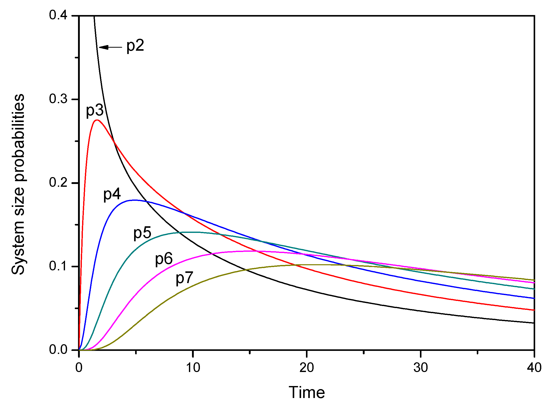
Transition probabilities for this model are computed with numerical values in Table 6 and time-dependent system size probabilities for model(a) are plotted in Figure 1.

Table 6. Transition probabilities for model(a), with $p=2k+2.5$, $q=0.2$, $N=10$.

m	r	${\mathit{p}}_{\mathit{m},\mathit{r}}\left(1\right)$	${\mathit{p}}_{\mathit{m},\mathit{r}}\left(5\right)$	${\mathit{p}}_{\mathit{m},\mathit{r}}\left(10\right)$	${\mathit{p}}_{\mathit{m},\mathit{r}}\left(15\right)$	${\mathit{p}}_{\mathit{m},\mathit{r}}\left(20\right)$	${\mathit{p}}_{\mathit{m},\mathit{r}}\left(25\right)$	${\mathit{p}}_{\mathit{m},\mathit{r}}\left(30\right)$
1	2	0.2921490112	0.2361484997	0.1522190975	0.1072492705	0.08052549270	0.06306134397	0.05080189081
	3	0.08716742291	0.2132663566	0.1738894810	0.1346557113	0.1065579573	0.08641940405	0.07149194738
	5	0.00238032673	0.08378329415	0.1339337865	0.1354764126	0.1240258026	0.1104448910	0.09768734107
	7	0.00002430702	0.01601707595	0.06178924538	0.08982065195	0.1002648982	0.1012550939	0.09777580080
2	2	0.4687113670	0.1946394431	0.1291172295	0.09425915593	0.07241108386	0.05755657124	0.04682820943
	3	0.2603710210	0.2132973859	0.1571127893	0.1219534631	0.09755450156	0.07987002622	0.06655452399
	4	0.07401956616	0.1794384547	0.1598844328	0.1349421989	0.1136304110	0.09641486357	0.08256032205
	5	0.01387332775	0.1205803453	0.1411610078	0.1327425518	0.1190445276	0.1053936555	0.09312573082
3	3	0.4666402935	0.1885109146	0.1333550248	0.1050671356	0.08556482599	0.07106591813	0.05985421345
	4	0.2468602213	0.1974994012	0.1489883379	0.1221831980	0.1027761281	0.08763755703	0.07546816996
	5	0.06813638099	0.1623296273	0.1451025641	0.1270522000	0.1115151393	0.09815261276	0.08668459066
	6	0.01252210876	0.1074754172	0.1250247001	0.1202487741	0.1114387753	0.1018850330	0.09263129043
5	2	0.0000964846760	0.0004029736173	0.0001109421737	0.00002487661389	0.000006292446081	0.000001903841593	6.850542824 (−7)
	5	0.4209957064	0.06081681946	0.01238287855	0.003239382078	0.001017418311	0.0003745677399	0.0001569887786
	6	0.3398204028	0.1224310542	0.02808273894	0.007687593257	0.002460489906	0.0009101597456	0.0003817757263
	8	0.0415780272	0.2028401500	0.08635305934	0.02965021464	0.01063284278	0.004185138909	0.001821109112

Figure 1. Time-dependent system size probabilities pr$:=p_{2,r}\left(t\right)$ in time t for model(a) with $m=2$, $p=2k+2.5$, $q=0.2$, $N=10$ and $r=2,3,4,5,6,7$.

5.2. Model(b)

$$\begin{array}{ccc}\hfill {\lambda }_n& =& {\displaystyle \frac{(p-2n)(p-n-1)}{p(p-2n-1)}}\hfill \\ \hfill {\mu }_n& =& {\displaystyle \frac{n(p-2n-2)}{p(p-2n-1)}},n\ge 1,p>2n+2\hfill \\ \hfill {\lambda }_0& =& 1,{\mu }_0=0\hfill \end{array}$$

It can be easily seen that ${\lambda }_n\ge 0$ and ${\mu }_n\ge 0$ for $n\ge 0$. Furthermore, ${\lambda }_n+{\mu }_n=1$ and

$${\lambda }_{n-1}{\mu }_n=\frac{n(p-2n-2)}{p(p-2n-1)}\left(1-\frac{(n-1)(p-2n)}{p(p-2n+1)}\right)$$

which is the chain sequence related to R-Bessel polynomials.

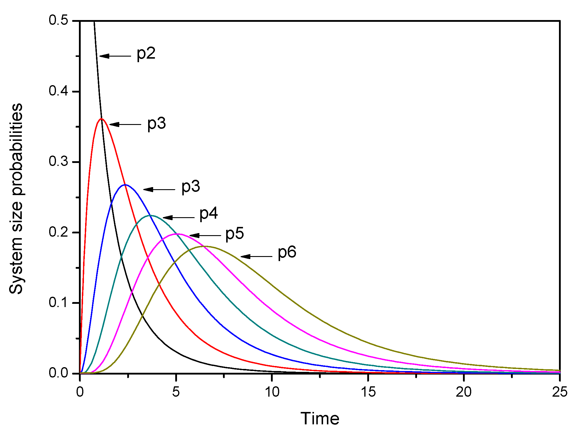
Transition probabilities for this model are computed with numerical values in Table 7.

Table 7. Transition probabilities for model(b), with $p=2k+2.5$, $N=10$.

m	r	${\mathit{p}}_{\mathit{m},\mathit{r}}\left(1\right)$	${\mathit{p}}_{\mathit{m},\mathit{r}}\left(5\right)$	${\mathit{p}}_{\mathit{m},\mathit{r}}\left(10\right)$	${\mathit{p}}_{\mathit{m},\mathit{r}}\left(15\right)$	${\mathit{p}}_{\mathit{m},\mathit{r}}\left(20\right)$	${\mathit{p}}_{\mathit{m},\mathit{r}}\left(25\right)$	${\mathit{p}}_{\mathit{m},\mathit{r}}\left(30\right)$
	2	0.3668649512	0.07064456326	0.006122786352	0.0007672220517	0.0001418440957	0.00003666418262	0.00001214606363
1	3	0.1701546382	0.1407243071	0.01888675760	0.002811271418	0.0005568489677	0.0001468292158	0.00004891825431
	4	0.0514906594	0.1941662333	0.04309915220	0.007886154548	0.001711514829	0.0004670552694	0.0001572694753
	5	0.011469638	0.2027097044	0.07762512167	0.01796275083	0.004359471899	0.001249481701	0.0004285528284
	2	0.3996490201	0.03099278684	0.003026111462	0.0004488996456	0.00009492395743	0.00002695810522	0.000009473396079
2	3	0.3593382733	0.08604679375	0.01055212421	0.001724092631	0.0003786025130	0.0001084563680	0.00003828579884
	4	0.1613757455	0.1540740571	0.02712850599	0.005095887598	0.001188222539	0.0003474884220	0.0001234936488
	8	0.003519920	0.1095910381	0.1503713552	0.06828797038	0.02481924585	0.009082332113	0.003603371537
	2	0.002239066965	0.002137757004	0.0003764044042	0.00007070476114	0.00001648642933	0.000004821355533	0.000001713457916
4	3	0.04864064014	0.01377958392	0.002193064577	0.0004416671154	0.0001122602281	0.00003534534684	0.00001326656829
	4	0.4151999358	0.05131643936	0.008681826526	0.001953416698	0.0005483642480	0.0001866026873	0.00007398207589
	7	0.04213035014	0.2022873297	0.07641991533	0.02328205397	0.007537792533	0.002735338567	0.001118752499
	2	0.0000032881816	0.00006422126647	0.00002925499766	0.000008079660527	0.000002258345658	7.149512291 (−7)	2.617673046 (−7)
6	5	0.06542941236	0.02357301641	0.005407082951	0.001480178073	0.0004737455651	0.0001752432074	0.00007350753874
	6	0.4257098799	0.06962097613	0.01643030578	0.004860655269	0.001677931965	0.0006615582574	0.0002913915376
	8	0.1374600047	0.1855299209	0.06208661130	0.02088652821	0.007708531309	0.003156124400	0.001425209067

Time-dependent system size probabilities for model(b) are plotted in Figure 2.

Figure 2. Time-dependent system size probabilities pr$:=p_{2,r}\left(t\right)$ in time t for model(b) with $m=2$, $p=2k+2.5$, $N=10$ and $r=2,3,4,5,6.$

5.3. Model(c)

$$\begin{array}{ccc}\hfill {\lambda }_n& =& {\displaystyle \frac{(n+\alpha +1)}{(2n+\alpha +1)}},\alpha >-1,n\ge 1\hfill \\ \hfill {\mu }_n& =& {\displaystyle \frac{n}{2n+\alpha +1}},\hfill \\ \hfill {\lambda }_0& =& 1,{\mu }_0=0.\hfill \end{array}$$

It can be noted that ${\lambda }_n\ge 0$ and ${\mu }_n\ge 0$ for $n\ge 0$. Further ${\lambda }_n+{\mu }_n=1$ and

$${\lambda }_{n-1}{\mu }_n={\displaystyle \frac{n}{2n+\alpha +1}}\left(1-{\displaystyle \frac{n-1}{2n+\alpha -1}}\right)$$

which is the chain sequence related to Laguerre polynomials [13].

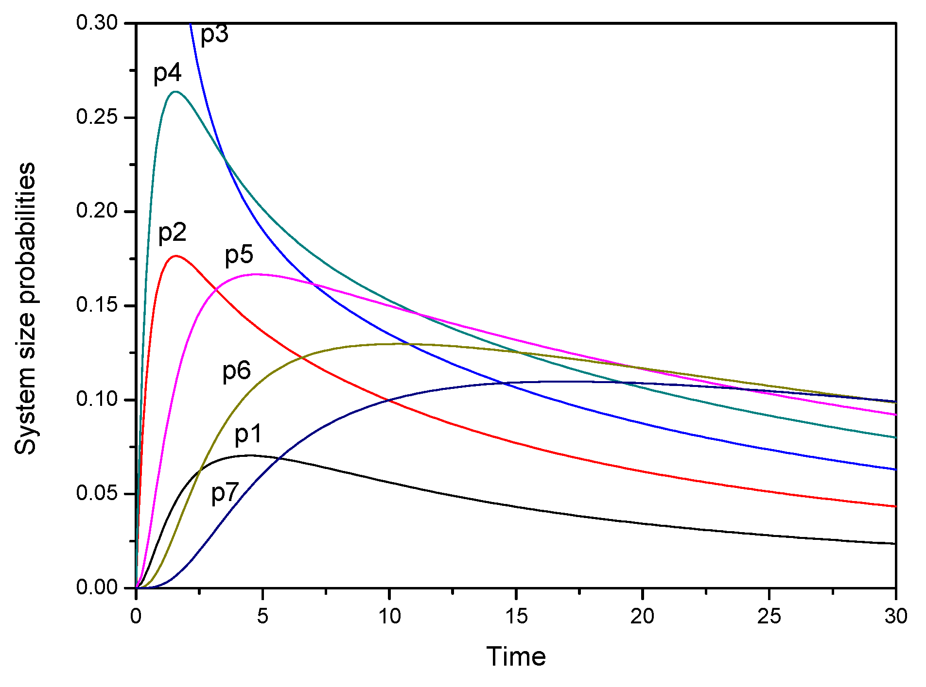
Transition probabilities for this model are computed with numerical values in Table 8.

Table 8. Transition probabilities for model(c), with $\alpha =0.5$, $N=10$.

m	r	${\mathit{p}}_{\mathit{m},\mathit{r}}\left(1\right)$	${\mathit{p}}_{\mathit{m},\mathit{r}}\left(5\right)$	${\mathit{p}}_{\mathit{m},\mathit{r}}\left(10\right)$	${\mathit{p}}_{\mathit{m},\mathit{r}}\left(15\right)$	${\mathit{p}}_{\mathit{m},\mathit{r}}\left(20\right)$	${\mathit{p}}_{\mathit{m},\mathit{r}}\left(25\right)$	${\mathit{p}}_{\mathit{m},\mathit{r}}\left(30\right)$
	2	0.4688267232	0.1928633801	0.1264207062	0.09218781872	0.07136666125	0.05757133172	0.04781824363
2	3	0.2653438205	0.2168648054	0.1584100418	0.1226725479	0.09856504753	0.08152856675	0.06897910514
	5	0.01443626936	0.1256558025	0.1467547469	0.1377028448	0.1236393294	0.1100037303	0.09802573107
	6	0.00201432251	0.06987523393	0.1153935846	0.1237887813	0.1197378807	0.1117862083	0.1030428725
	1	0.02917435854	0.07005180573	0.05612717942	0.04319081505	0.03424686358	0.02800919288	0.02349067590
3	2	0.1667875442	0.1363150204	0.09957202627	0.07710845857	0.06195517271	0.05124652764	0.04335829463
	3	0.4672718500	0.1903502007	0.1348745875	0.1065555416	0.08744076768	0.07355224355	0.06302933573
	6	0.01281660035	0.1106226948	0.1296802361	0.1253706875	0.1167654692	0.1074488453	0.09853498511
	1	0.004006093074	0.03490131784	0.03804604903	0.03301105450	0.02790196141	0.02374149645	0.02045846387
4	3	0.1753337072	0.1753337072	0.1072362467	0.08824142863	0.07467112357	0.06429071854	0.05610744881
	5	0.2409534358	0.1926145016	0.1456727717	0.1223972416	0.1067395368	0.09465581698	0.08478676156
	6	0.06540061567	0.1559532589	0.1395179853	0.1239369090	0.1116997349	0.1014857762	0.09267627585
5	1	0.000429767008	0.01498158082	0.02362958641	0.02372314186	0.02167960266	0.01936335494	0.01724682791
	3	0.03659875165	0.08779175077	0.07903155670	0.06950029549	0.06132142863	0.05439130069	0.04854685473
	5	0.4663702967	0.1861249691	0.1320798136	0.1091642271	0.09506946368	0.08469292916	0.07634551417
	6	0.2351733252	0.1871505923	0.1405394533	0.1181891252	0.1041888019	0.09388609320	0.08557504052

Time-dependent system size probabilities for model(c) are plotted in Figure 3.

Figure 3. Time-dependent system size probabilities pr$:=p_{3,r}\left(t\right)$ in time t for model(c) with $m=3$, $\alpha =0.5$, $N=10$ and $r=1,2,3,4,5,6,7$.

6. Birth and Death Processes Related to Modular Forms

In this section, we consider a special type of birth and death process with transition rates satisfying

$$\begin{array}{ccc}\hfill {\lambda }_n+{\mu }_n& =& 1+q^n\hfill \\ \hfill {\lambda }_{n-1}{\mu }_n& =& q^n\hfill \end{array}$$

where ${\lambda }_0=1$ and $q\in (0,1)$.

Now from (27) we have

$$\begin{array}{c}\hfill f_{0,0}\left(s\right)=\frac{1}{s+1-\frac{q}{s+q+1-\frac{q^2}{s+q^2+1-\cdots }}}.\end{array}$$

(36)

which is the modular form when $s=0$ [23] (p. 290, ex. 14)

$$\begin{array}{c}\hfill f_{0,0}\left(0\right)=\sum _{n=0}^{\infty }{q}^{n(n+1)/2}=\frac{1}{1-\frac{q}{q+1-\frac{q^2}{q^2+1-\cdots }}}.\end{array}$$

(37)

Transition probabilities for this model are computed with numerical values in Table 9.

Table 9. Transition probabilities with $q=0.3$, $N=10$.

m	r	${\mathit{p}}_{\mathit{m},\mathit{r}}\left(1\right)$	${\mathit{p}}_{\mathit{m},\mathit{r}}\left(5\right)$	${\mathit{p}}_{\mathit{m},\mathit{r}}\left(10\right)$	${\mathit{p}}_{\mathit{m},\mathit{r}}\left(15\right)$	${\mathit{p}}_{\mathit{m},\mathit{r}}\left(20\right)$	${\mathit{p}}_{\mathit{m},\mathit{r}}\left(25\right)$	${\mathit{p}}_{\mathit{m},\mathit{r}}\left(30\right)$
2	2	0.3900357047	0.02658584041	0.003251737369	0.0004999903630	0.00007840736855	0.00001231747087	0.000001935350659
	3	0.3756794991	0.06058285595	0.005664561651	0.0008170697324	0.0001272010066	0.00001996780969	0.000003137153307
	4	0.1859163290	0.1139863351	0.01033550057	0.001335267686	0.0002037521180	0.00003190719536	0.000005011638279
	6	0.03459111	0.1941578052	0.03413503594	0.003762703845	0.0005154609431	0.00007893180696	0.00001235816122
3	1	0.0004630194876	0.0004580759529	0.00008060843377	0.00001278455567	0.000002010595418	3.159439443 (−7)	4.964323829 (−8)
	2	0.01014334649	0.001635737113	0.0001529431649	0.00002206088278	0.000003434427186	5.391308622 (−7)	8.470313934 (−8)
	4	0.3701921713	0.03976083628	0.001070262814	0.00006825537042	0.000009072098519	0.000001398890914	2.193776390 (−7)
	5	0.1845293945	0.09157906054	0.003444466194	0.0001486194938	0.00001516582457	0.000002237431245	3.491270317 (−7)
4	2	0.00004065990305	0.00002492881147	0.000002260373975	2.920230428 (−7)	4.456058821 (−8)	6.978103621 (−9)	1.096045292 (−9)
	3	0.002998556596	0.0003220627739	0.000008669128788	5.528685000 (−7)	7.348399796 (−8)	1.133101637 (−8)	1.776958875 (−9)
	4	0.3698214230	0.007688259764	0.00007926891020	0.000001612886673	1.268093942 (−7)	1.823425381 (−8)	2.840614969 (−9)
	6	0.1841254981	0.08628876235	0.002513625449	0.00004505149497	9.149910149 (−7)	5.327583632 (−8)	7.116594456 (−9)

Time-dependent system size probabilities for this model are plotted in Figure 4.

Figure 4. Time-dependent system size probabilities pr$:=p_{2,r}\left(t\right)$ in time t with $m=2$, $N=10$ and $r=2,3,4,5,6$.

7. Conclusions

This article finds bounds for the zeros of classical polynomials that are related to birth and death processes. As an application, transition probabilities related to g-fractions and modular forms are derived. The results are validated through numerical examples. Three different models have been considered and numerical values of transition probabilities have been computed for those models.