
Improving Sparrow Search Algorithm for Optimal Operation Planning of Hydrogen–Electric Hybrid Microgrids Considering Demand Response

Abstract
:1. Introduction
2. Demand Response Model
2.1. Demand Response Objective Function
2.2. User Satisfaction Function
2.3. Demand Response Constraints
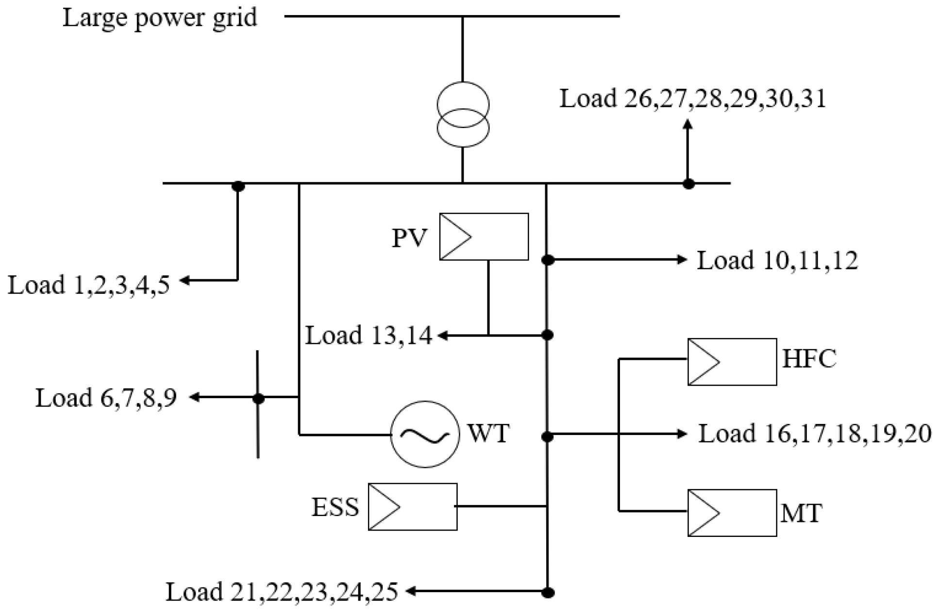
3. Hydrogen–Electric Hybrid Microgrid Model
3.1. Objective Function of Microgrid
3.2. Distributed Energy Resources Model
3.3. Constraints of DER
4. Algorithm for Solving the Optimization Model
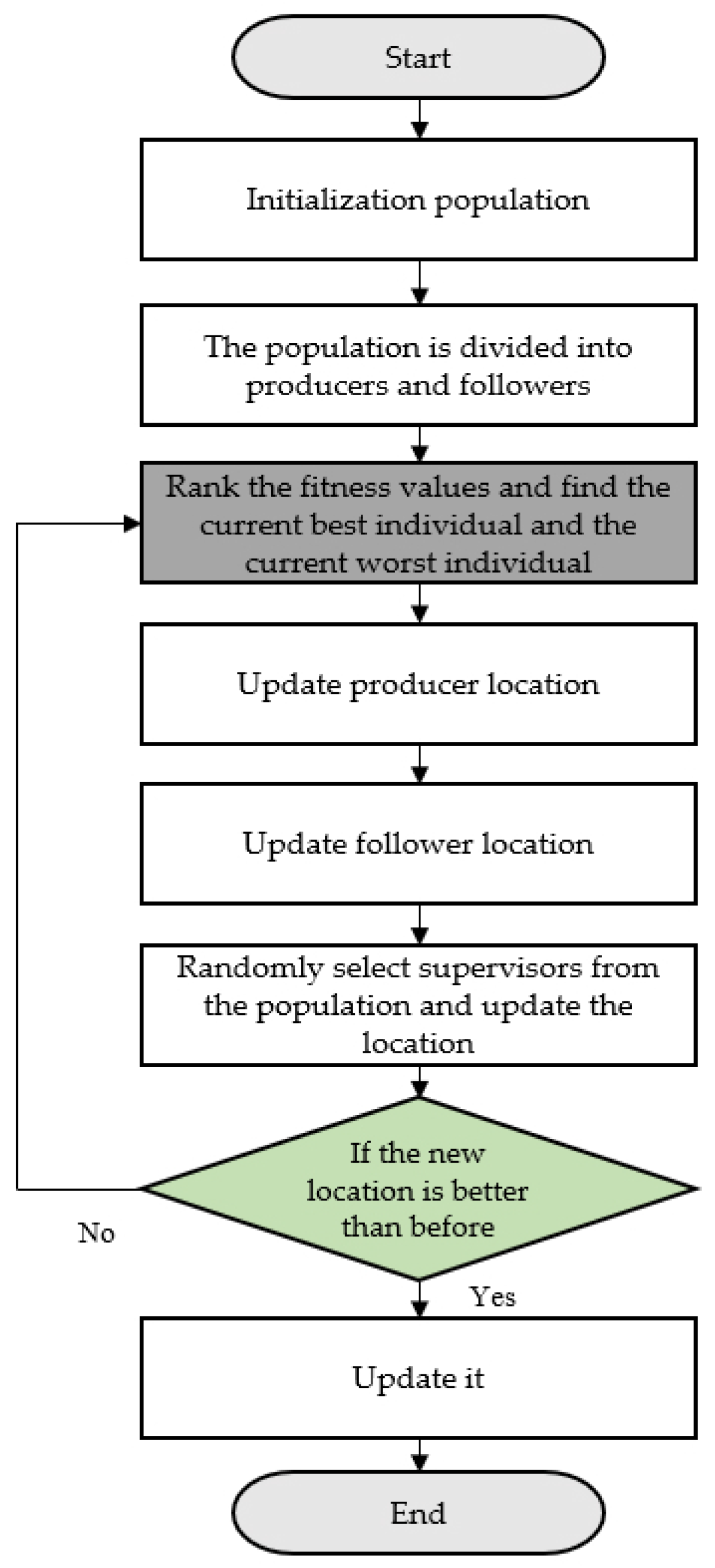
4.1. Improved Sparrow Search Algorithm
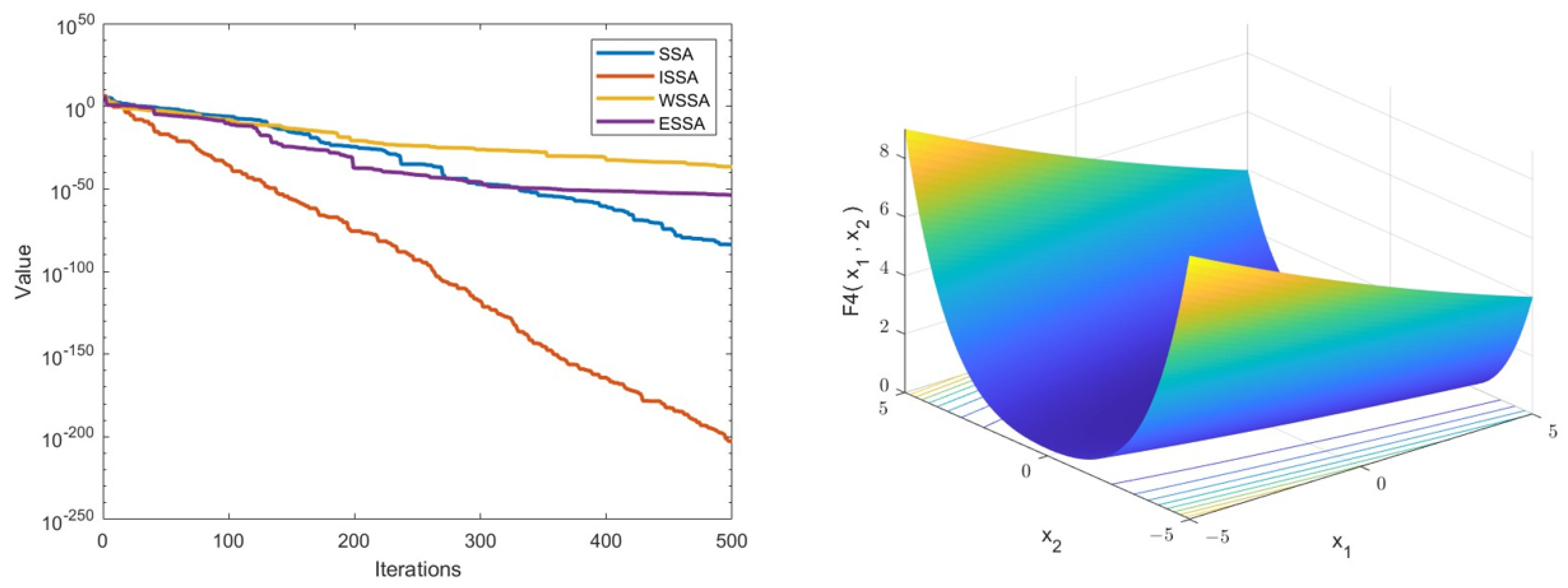
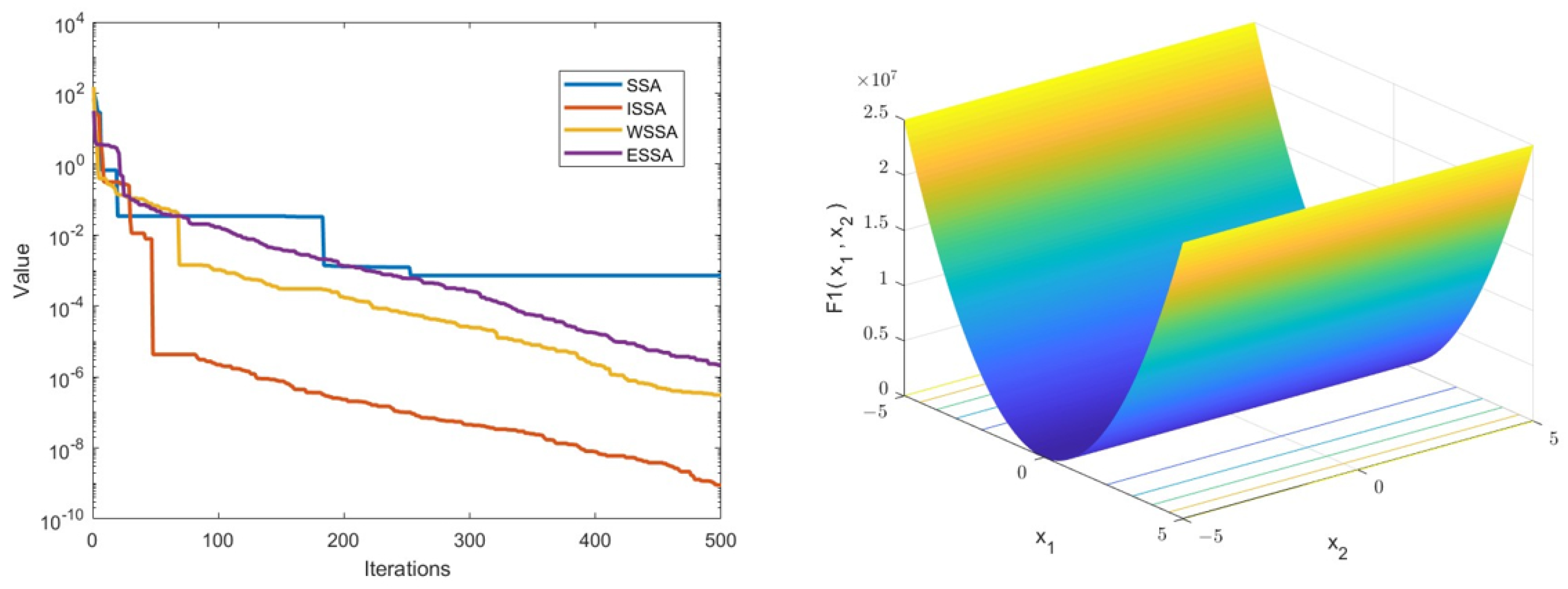
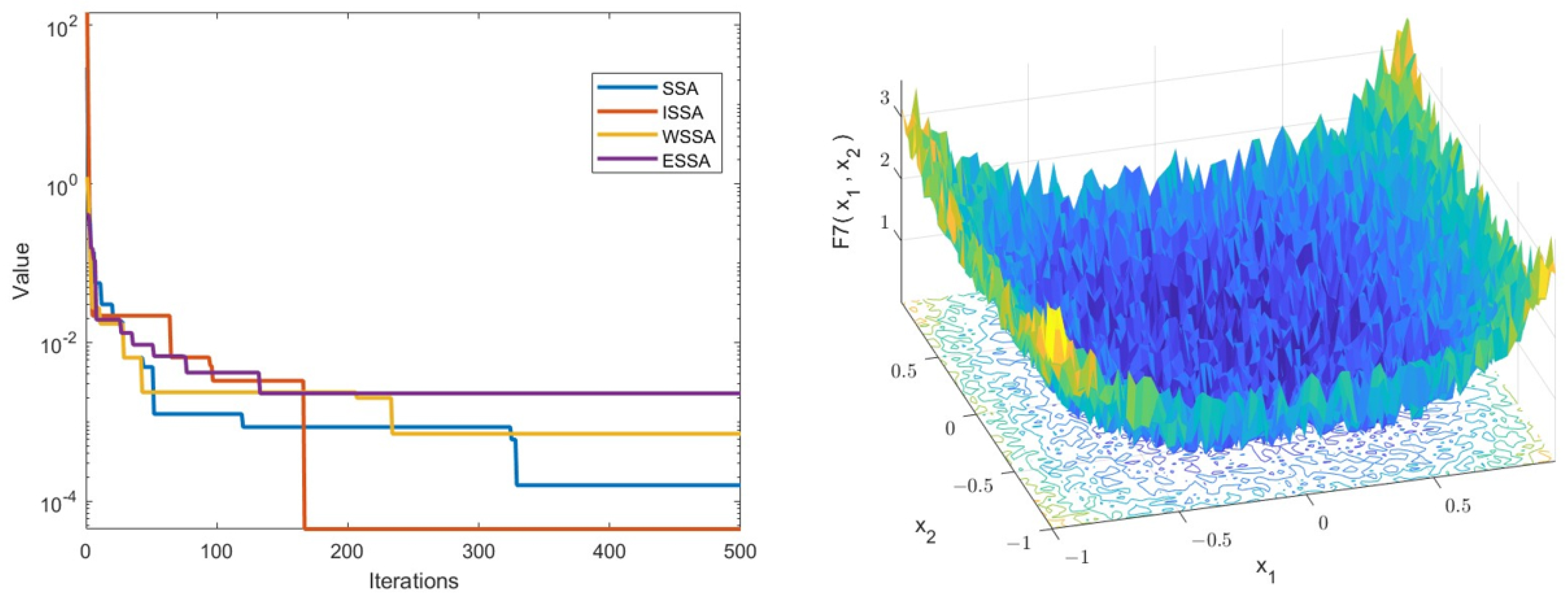
4.2. Test Function
| Algorithm 1 Pseudocode of ISSA. |
| Require: T: the maximum iterations : the number of producers : the number of sparrows who perceive danger : the alarm value n: the number of sparrows Initialize a population of n sparrows and define its relevant Parameters Ensure: , 1: whiledo 2: Rank the fitness values and find the current best individual and the current worst individual. 3: = 4: for do i = 1:PD 5: Using Equation (30) update the sparrow’s location; 6: end for 7: for do i = (PD + 1):n 8: Using Equation (26) update the sparrow’s location; 9: end for 10: for = 1:SD 11: Using Equation (31) update the sparrow’s location; 12: end for 13: Get the current new location; 14: If the new location is better than before, update it 15: t = 16: end while 17: return , |
5. Calculation and Analysis
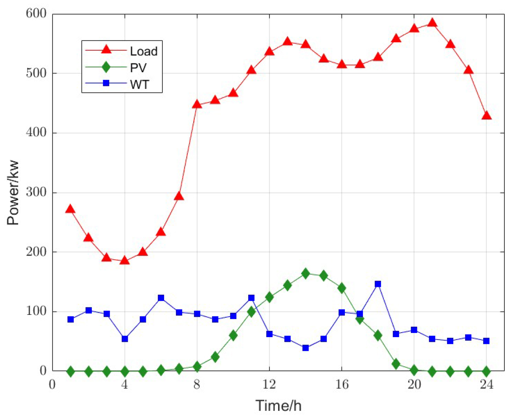
5.1. Related Calculation and Analysis Data
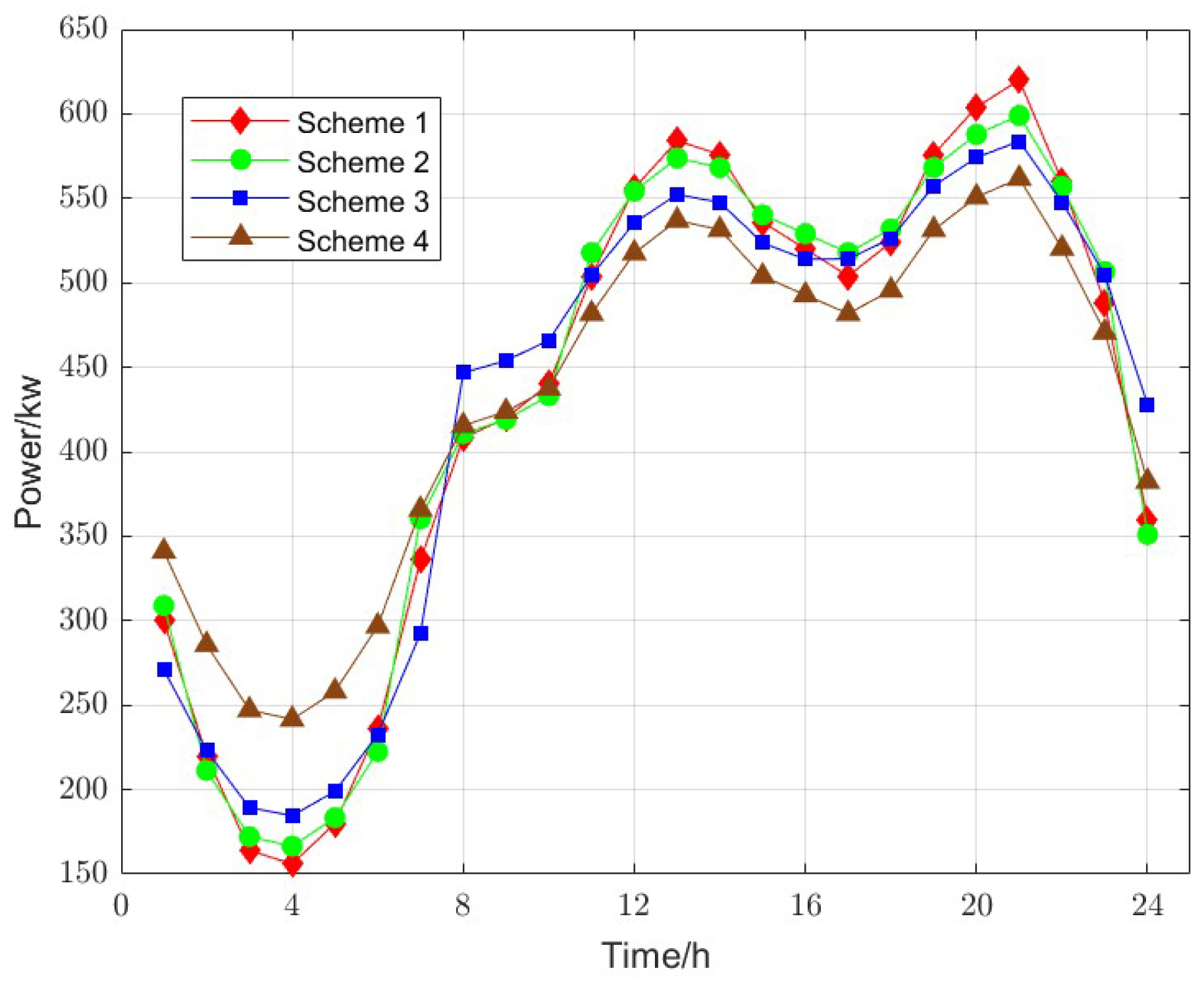
5.2. Analysis of Demand Response Results
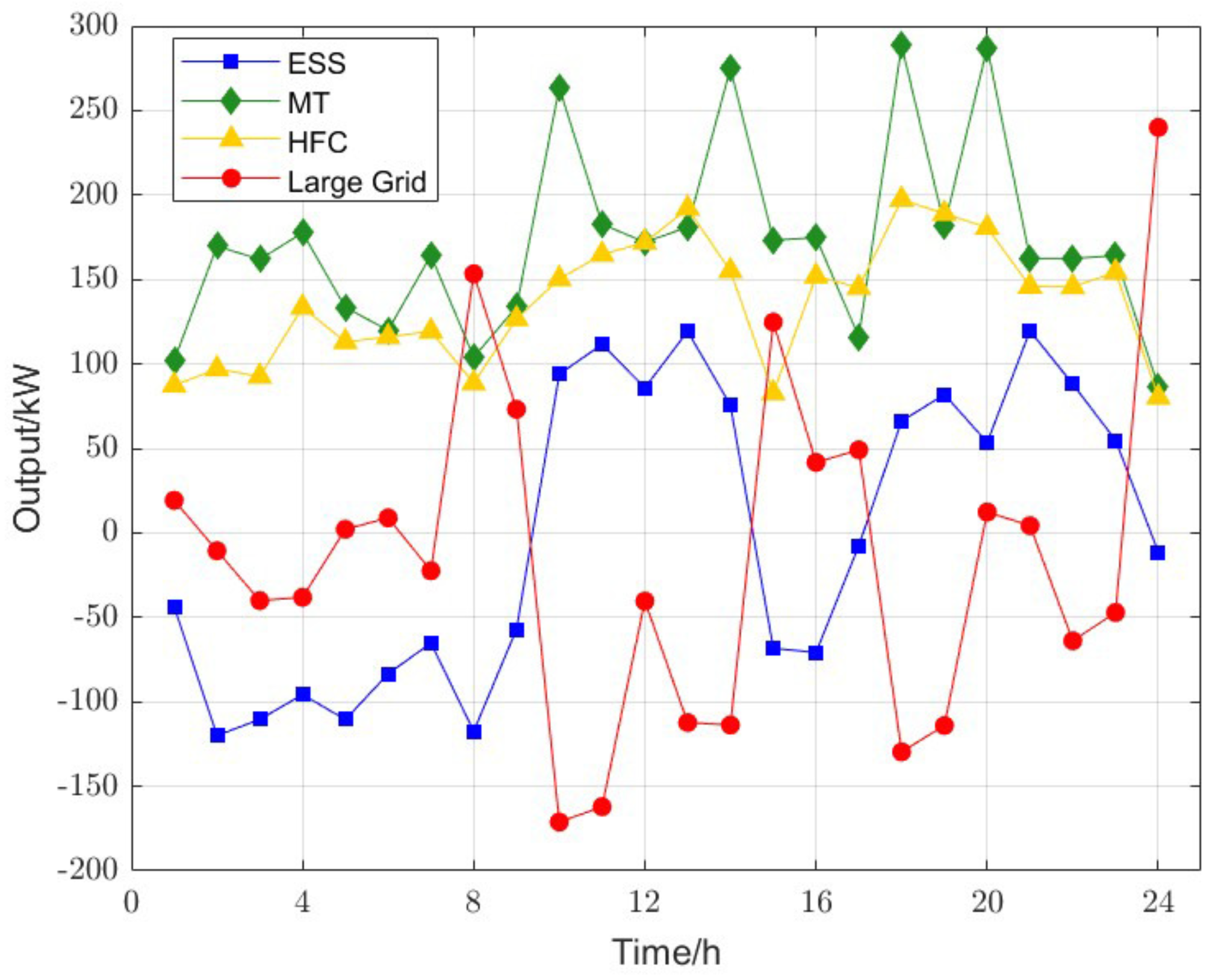
5.3. Analysis of Demand Response Results
6. Conclusions
Author Contributions
Funding
Institutional Review Board Statement
Informed Consent Statement
Data Availability Statement
Conflicts of Interest
References
- Li, X.; Fang, L. Research on economic dispatch of large power grid based on granular computing. In Proceedings of the 2016 IEEE PES Asia-Pacific Power and Energy Engineering Conference (APPEEC), Xi’an, China, 25–28 October 2016; pp. 1130–1133. [Google Scholar] [CrossRef]
- Qin, X.; Su, L.; Jiang, Y.; Zhou, Q.; Chen, J.; Xu, X.; Chi, Y.; An, N. Study on inertia support capability and its impact in large scale power grid with increasing penetration of renewable energy sources. In Proceedings of the 2018 International Conference on Power System Technology (POWERCON), Guangzhou, China, 6–8 November 2018; pp. 1018–1024. [Google Scholar] [CrossRef]
- Liu, L.; Wei, K.; Ge, X. GIC in Future Large-Scale Power Grids: An analysis of the problem. IEEE Electrif. Mag. 2015, 3, 52–59. [Google Scholar] [CrossRef]
- Du, W.; Tuffner, F.K.; Schneider, K.P.; Lasseter, R.H.; Xie, J.; Chen, Z.; Bhattarai, B. Modeling of grid-forming and grid-following inverters for dynamic simulation of large-scale distribution systems. Atmosphere 2021, 12, 1086. [Google Scholar] [CrossRef]
- Maciejczyk, P.; Chen, L.; Thurston, G. The role of fossil fuel combustion metals in PM2.5 air pollution health associations. IEEE Trans. Power Deliv. 2020, 36, 2035–2045. [Google Scholar] [CrossRef]
- Perera, F. Pollution from fossil-fuel combustion is the leading environmental threat to global pediatric health and equity: Solutions exist. Int. J. Environ. Res. Public Health 2018, 15, 16. [Google Scholar] [CrossRef] [Green Version]
- Perera, F. Multiple threats to child health from fossil fuel combustion: Impacts of air pollution and climate change. Environ. Health Perspect. 2017, 125, 141–148. [Google Scholar] [CrossRef] [PubMed] [Green Version]
- Fu, X.; Sun, J.; Huang, M.; Tian, Z.; Yan, H.; Iu, H.H.; Hu, P.; Zha, X. Large-signal stability of grid-forming and grid-following controls in voltage source converter: A comparative study. IEEE Trans. Power Electron. 2020, 36, 7832–7840. [Google Scholar] [CrossRef]
- Zhang, Y.; Jin, L.; Wang, Y.; Liu, H. The Exploration and Application Research of Emerging Technologies in Operation and Maintenance of Large Power Grid Enterprises. IOP Conf. Ser. Mater. Sci. Eng. 2016, 688, 055090. [Google Scholar] [CrossRef]
- Ghasemi, A.; Enayatzare, M. Optimal energy management of a renewable-based isolated microgrid with pumped-storage unit and demand response. Renew. Energy 2018, 123, 460–474. [Google Scholar] [CrossRef]
- Zia, M.F.; Elbouchikhi, E.; Benbouzid, M. Microgrids energy management systems: A critical review on methods, solutions, and prospects. Appl. Energy 2018, 222, 1033–1055. [Google Scholar] [CrossRef]
- Mengelkamp, E.; Gärttner, J.; Rock, K.; Kessler, S.; Orsini, L.; Weinhardt, C. Designing microgrid energy markets: A case study: The Brooklyn Microgrid. Appl. Energy 2018, 210, 870–880. [Google Scholar] [CrossRef]
- Kaur, A.; Kaushal, J.; Basak, P. A review on microgrid central controller. Renew. Sustain. Energy Rev. 2016, 55, 338–345. [Google Scholar] [CrossRef]
- Wan, X.; Lian, H.; Ding, X.; Peng, J.; Wu, Y.; Li, X. Hierarchical multiobjective dispatching strategy for the microgrid system using modified MOEA/D. Complexity 2020, 2020, 4725808. [Google Scholar] [CrossRef]
- Tian, L.; Cheng, L.; Guo, J.; Wu, K. System modeling and optimal dispatching of multi-energy microgrid with energy storage. J. Mod. Power Syst. Clean Energyy 2020, 8, 809–819. [Google Scholar] [CrossRef]
- Jiang, H.; Ning, S.; Ge, Q. Multi-objective optimal dispatching of microgrid with large-scale electric vehicles. IEEE Access 2019, 1, 145880–145888. [Google Scholar] [CrossRef]
- Dou, C.; Zhou, X.; Zhang, T.; Xu, S. Economic optimization dispatching strategy of microgrid for promoting photoelectric consumption considering cogeneration and demand response. J. Mod. Power Syst. Clean Energy 2020, 8, 557–563. [Google Scholar] [CrossRef]
- Hosseini, S.M.; Carli, R.; Dotoli, M. Robust optimal energy management of a residential microgrid under uncertainties on demand and renewable power generation. IEEE Trans. Autom. Sci. Eng. 2020, 18, 618–637. [Google Scholar] [CrossRef]
- Muhtadi, A.; Pandit, D.; Nguyen, N.; Mitra, J. Distributed energy resources based microgrid: Review of architecture, control, and reliability. IEEE Trans. Ind. Appl. 2021, 57, 2223–2235. [Google Scholar] [CrossRef]
- Al-Ismail, F.S. DC microgrid planning, operation, and control: A comprehensive review. IEEE Access 2021, 9, 36154–36172. [Google Scholar] [CrossRef]
- Ali, S.; Zheng, Z.; Aillerie, M.; Sawicki, J.; Pera, M.; Hissel, D. A review of DC Microgrid energy management systems dedicated to residential applications. Energies 2021, 14, 4308. [Google Scholar] [CrossRef]
- Akinyele, D.; Olabode, E.; Amole, A. Review of fuel cell technologies and applications for sustainable microgrid systems. Inventions 2020, 5, 42. [Google Scholar] [CrossRef]
- Beheshtaein, S.; Cuzner, R.M.; Forouzesh, M.; Savaghebi, M.; Guerrero, J.M. DC microgrid protection: A comprehensive review. IEEE J. Emerg. Sel. Top. Power Electron. 2019, 1, 1. [Google Scholar] [CrossRef]
- Lorestani, A.; Gharehpetian, G.B.; Nazari, M.H. Optimal sizing and techno-economic analysis of energy-and cost-efficient standalone multi-carrier microgrid. Energy 2019, 178, 751–764. [Google Scholar] [CrossRef]
- Oghaddas-Tafreshi, S.M.; Mohseni, S.; Karami, M.E.; Kelly, S. Optimal energy management of a grid-connected multiple energy carrier micro-grid. Appl. Therm. Eng. 2019, 152, 796–806. [Google Scholar] [CrossRef]
- Cui, C.; Dong, Z. Optimal Operation Strategy of Microgrid Based on TD3 Algorithm. In Proceedings of the 2022 7th International Conference on Power and Renewable Energy (ICPRE), Shanghai, China, 23–26 September 2022; pp. 347–351. [Google Scholar] [CrossRef]
- Deng, H.; Li, B.; Wang, J.; Hu, W. Multi-objective optimal dispatching of microgrid considering demand side response. In Proceedings of the International Conference on Mechanisms and Robotics (ICMAR 2022), Zhuhai, China, 10 November 2022; pp. 633–639. [Google Scholar] [CrossRef]
- Rajagopalan, A.; Nagarajan, K.; Montoya, O.D.; Dhanasekaran, S.; Kareem, I.A.; Perumal, A.S.; Lakshmaiya, N.; Paramasivam, P. Multi-Objective Optimal Scheduling of a Microgrid Using Oppositional Gradient-Based Grey Wolf Optimizer. Energies 2022, 15, 9024. [Google Scholar] [CrossRef]
- Arumugam, P.; Kuppan, V. A GBDT-SOA approach for the system modelling of optimal energy management in grid-connected micro-grid system. Int. J. Energy Res. 2021, 45, 6765–6783. [Google Scholar] [CrossRef]
- Gad, Y.; Diab, H.; Abdelsalam, M.; Galal, Y. Smart energy management system of environmentally friendly microgrid based on grasshopper optimization technique. Energies 2020, 13, 5000. [Google Scholar] [CrossRef]
- Karthik, N.; Parvathy, A.K.; Arul, R.; Jayapragash, R.; Narayanan, S. Economic load dispatch in a microgrid using Interior Search Algorithm. In Proceedings of the 2019 Innovations in Power and Advanced Computing Technologies (i-PACT), Vellore, India, 22–23 March 2019; pp. 1–6. [Google Scholar] [CrossRef]
- Nguyen, T.; Ngo, T.; Dao, T.; Nguyen, T. Microgrid operations planning based on improving the flying sparrow search algorithm. Symmetry 2022, 14, 168. [Google Scholar] [CrossRef]
- Liu, Y.; Yang, S.; Li, D.; Zhang, S. Improved Whale Optimization Algorithm for Solving Microgrid Operations Planning Problems. Symmetry 2022, 15, 36. [Google Scholar] [CrossRef]
- Khodaei, A. Provisional microgrids. IEEE Trans. Smart Grid. 2014, 6, 1107–1115. [Google Scholar] [CrossRef]
- Khodaei, A. Provisional microgrid planning. IEEE Trans. Smart Grid 2015, 8, 1096–1104. [Google Scholar] [CrossRef]
- Wu, Q.; Xie, Z.; Ren, H.; Li, Q.; Yang, Y. Optimal trading strategies for multi-energy microgrid cluster considering demand response under different trading modes: A comparison study. Energy 2022, 254, 124448. [Google Scholar] [CrossRef]
- Xue, J.; Shen, B. A novel swarm intelligence optimization approach: Sparrow search algorithm. Syst. Sci. Control Eng. 2020, 15, 22–34. [Google Scholar] [CrossRef]
- Wu, G.; Mallipeddi, R.; Suganthan, P.N. Problem Definitions and Evaluation Criteria for the CEC 2017 Competition on Constrained Real-Parameter Optimization; Technical Report; National University of Defense Technology: Changsha, China; Kyungpook National University: Daegu, Republic of Korea; Nanyang Technological University: Singapore, 2017. [Google Scholar]
- Seel, J.; Mills, A.; Millstein, D.; Gorman, W.; Jeong, S. Solar-to-Grid Public Data File for Utility-scale (UPV) and Distributed Photovoltaics (DPV) Generation, Capacity Credit, and Value. 2020. Available online: https://data.openei.org/submissions/2881 (accessed on 30 November 2022).
- Thibedeau, J. July 2014 Green Machine Florida Canyon Hourly Data. 2014. Available online: https://gdr.openei.org/submissions/431 (accessed on 30 November 2022).
- Nguyen, T.; Dao, T.; Nguyen, T. An Optimal Microgrid Operations Planning Using Improved Archimedes Optimization Algorithm. IEEE Access 2022, 10, 67940–67957. [Google Scholar] [CrossRef]
- Zhang, Z.; Wang, Z.; Wang, H.; Zhang, H.; Yang, W.; Cao, R. Research on bi-level optimized operation strategy of microgrid cluster based on IABC algorithm. IEEE Access 2021, 9, 15520–15529. [Google Scholar] [CrossRef]


| Algorithm | Equation |
|---|---|
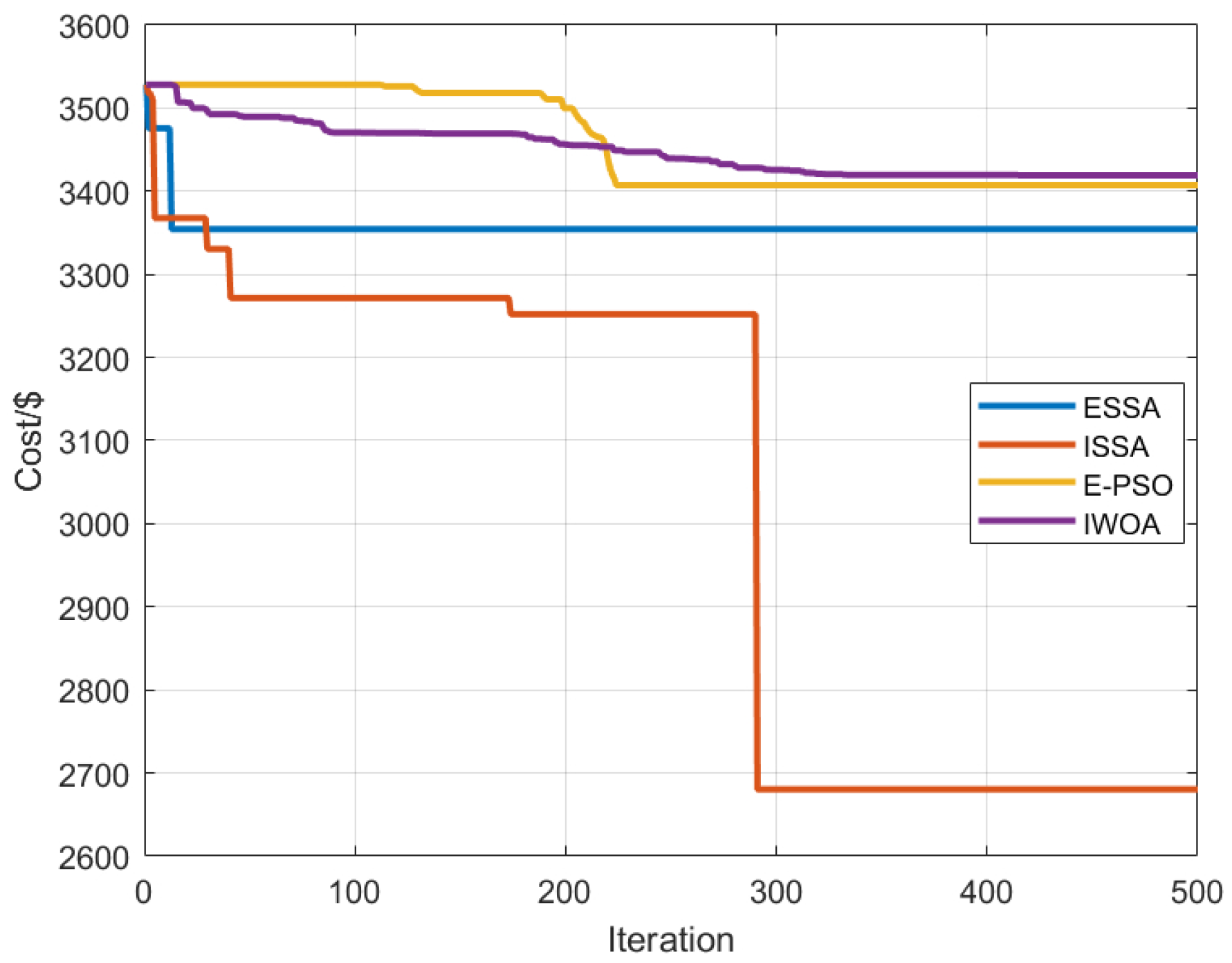
| Algorithms | SSA | WSSA | ESSA | ISSA |
|---|---|---|---|---|
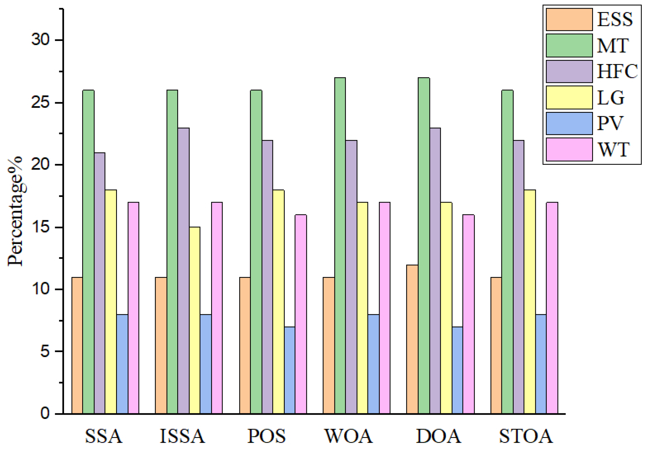
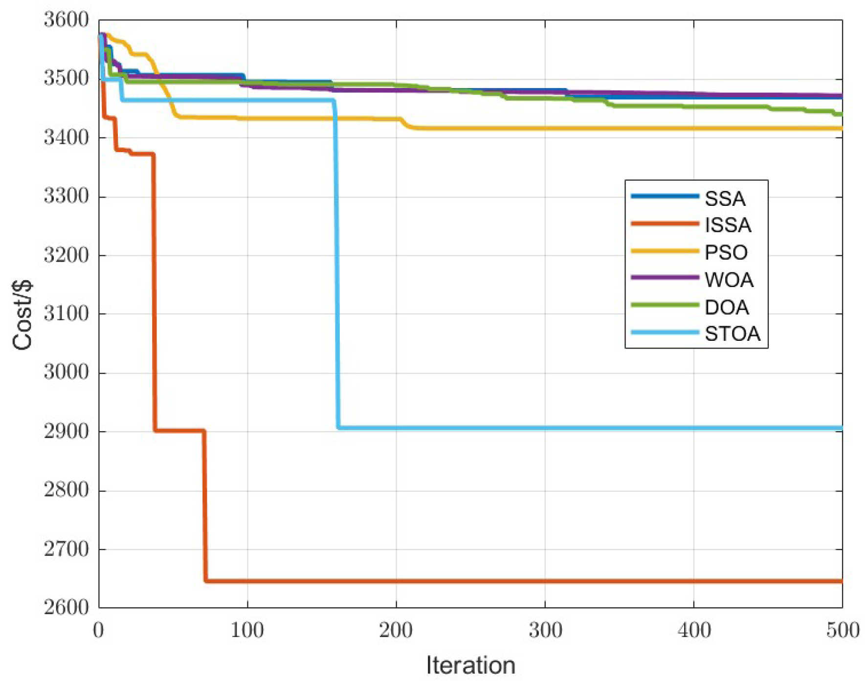
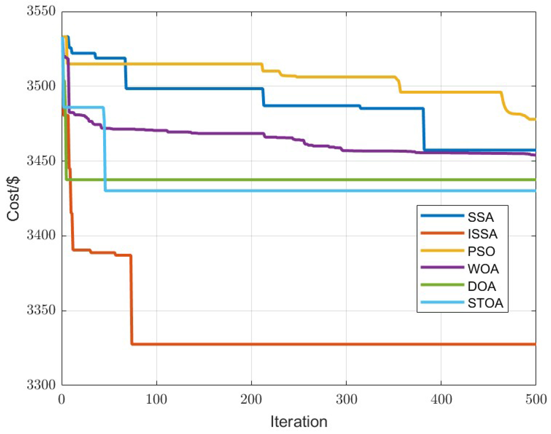
| Algorithms | POS | WOA | DOA | STOA | ISSA |
|---|---|---|---|---|---|
| Types | Price/[USD·(kWh)] | ||
|---|---|---|---|
| Peak Period | Through Period | Normal Period | |
| Buy | 0.84 | 0.19 | 0.51 |
| Sell | 0.42 | 0.10 | 0.26 |
| Types | Minimum Power/(kW) | Maximum Power/(kW) | Maintenance Costs/(USD/kW) | Climb Rates/(kW/min) |
|---|---|---|---|---|
| Large Grid | −240 | 240 | 0.001 | / |
| PV | 0 | 180 | 0.012 | / |
| WT | 0 | 170 | 0.036 | / |
| MT | 15 | 300 | 0.107 | 2 |
| HFC | 5 | 250 | 0.205 | 3 |
| ESS | −150 | 150 | 0.005 | / |
| Types of Pollutant | Pollution Costs (USD/kg) | Emission Factors of MT/(kg/kWh) |
|---|---|---|
| CO | 0.0041 | 0.184 |
| SO | 0.875 | 9.3 × 10 |
| NO | 1.25 | 6.19 × 10 |
| CO | 0.145 | 1.7 × 10 |
| Schemes | Electricity Satisfaction | Compensation for Demand Response/(USD) | Comprehensive Operation Cost/(USD) | ||
|---|---|---|---|---|---|
| Strategy 1 | Strategy 2 | Strategy 3 | |||
| 1 | 100% | 0 | 3420.91 | 3692.82 | 3301.26 |
| 2 | 96.53% | 175.39 | 3349.65 | 3619.77 | 3212.14 |
| 3 | 94.14% | 298.63 | 3246.34 | 3510.24 | 3121.83 |
| 4 | 89.39% | 425.13 | 3224.39 | 3473.64 | 3098.49 |
| Types of Algorithms | Cost/(USD) | ||
|---|---|---|---|
| Worst | Best | Average | |
| SSA | 3482.29 | 3225.77 | 3341.36 |
| ISSA | 3327.41 | 2647.34 | 2879.53 |
| POS | 3456.25 | 3194.27 | 3320.51 |
| WOA | 3490.26 | 3165.27 | 3297.19 |
| DOA | 3493.65 | 3050.44 | 3145.73 |
| STOA | 3401.53 | 2851.26 | 3014.59 |
| ESSA | 3469.36 | 3259.71 | 3376.29 |
| E-PSO | 3503.64 | 3186.82 | 3324.76 |
| IWOA | 3486.62 | 3094.36 | 3256.73 |
Disclaimer/Publisher’s Note: The statements, opinions and data contained in all publications are solely those of the individual author(s) and contributor(s) and not of MDPI and/or the editor(s). MDPI and/or the editor(s) disclaim responsibility for any injury to people or property resulting from any ideas, methods, instructions or products referred to in the content. |
© 2023 by the authors. Licensee MDPI, Basel, Switzerland. This article is an open access article distributed under the terms and conditions of the Creative Commons Attribution (CC BY) license (https://creativecommons.org/licenses/by/4.0/).
Share and Cite
Zhao, Y.; Liu, Y.; Wu, Z.; Zhang, S.; Zhang, L. Improving Sparrow Search Algorithm for Optimal Operation Planning of Hydrogen–Electric Hybrid Microgrids Considering Demand Response. Symmetry 2023, 15, 919. https://doi.org/10.3390/sym15040919
Zhao Y, Liu Y, Wu Z, Zhang S, Zhang L. Improving Sparrow Search Algorithm for Optimal Operation Planning of Hydrogen–Electric Hybrid Microgrids Considering Demand Response. Symmetry. 2023; 15(4):919. https://doi.org/10.3390/sym15040919
Chicago/Turabian StyleZhao, Yuhao, Yixing Liu, Zhiheng Wu, Shouming Zhang, and Liang Zhang. 2023. "Improving Sparrow Search Algorithm for Optimal Operation Planning of Hydrogen–Electric Hybrid Microgrids Considering Demand Response" Symmetry 15, no. 4: 919. https://doi.org/10.3390/sym15040919