MHD Stagnation Point of Blasius Flow for Micropolar Hybrid Nanofluid toward a Vertical Surface with Stability Analysis

Abstract

This study investigates the magnetohydrodynamics of a micropolar fluid consisting of a hybrid nanofluid with mixed convection effects. By using the dimensionless set of variables, the resulting equations of ordinary differential equations are solved numerically using the bvp4c solver in MATLAB. In the present work, the water-based alumina–copper hybrid nanofluid is analytically modeled with modified thermophysical properties. The study reveals that the highest critical value of opposing flow is the hybrid nanofluid (ϕ₁ = ϕ₂ = 2%). By comparing the hybrid nanofluid with Cu–water nanofluid (ϕ₁ = 0%, ϕ₂ = 1%) as well as water (ϕ₁ = 0%, ϕ₂ = 0%), hybrid nanoparticle volume fraction enhances the dynamic viscosity performance and surface shear stress. In addition, the augmentation of the nanoparticle volume fraction and magnetic field parameter will increase the physical quantities Re_x^1/2 C_f, Re_x M_x, and Re_x^−1/2 Nu_x. The result from the stability inquiry discloses that the first solution is more physically stable and trustworthy. It is proven that magnetohydrodynamics could contribute to controlling the fluid flow in a system, i.e., engineering operations and the medical field. In addition, this theoretical research can be a benchmark for experimental research.

1. Introduction

Recently, micropolar fluid (MF) issues have gained the attention of many researchers due to their various applications in pharmaceutical, chemical, food processing, and engineering industries, such as the solidification of liquid crystals, lubricant in the journal bearing, colloidal solutions, and many more [1]. In addition, this MF model can be used to explain the flow of colloidal solutions, liquid crystals, suspension solutions, animal blood, etc. This is because the equation governing the flow of an MF involves a microrotation vector and a gyration parameter in addition to the classical velocity vector field. Eringen [2] was the pioneer who proposed the theory of MF. His approach is based on rotating particles. The rotation is called a self-reliant microrotation vector. This theory also considers the structure and movement of micro fluids as well as it can explain the behavior of fluid flow that cannot be explained by Newtonian’s classical theory of fluids. Ishak [3] utilized the Runge–Kutta–Fehlberg (RKF) method to determine how radiation affected the thermal boundary layer flow caused by a linearly stretched sheet submerged in an incompressible MF with a constant wall temperature. He discovered that the presence of radiation causes the heat transfer rate (HTR) at the surface to decrease. Aurangzaib et al. [4] analyzed the boundary layer flow of MF and heat transfer over an exponentially permeable shrinking sheet and found that when the material parameter increased, the velocity decreased for the first outcome but increased for the second outcome. However, the effects of fluid temperature are the opposite.

There are several studies regarding the MF related to the stagnation point flow have been carried out by Nazar et al. [5], Nadeem et al. [6], Ishak et al. [7], Noor et al. [8] and Ul Haq et al. [9]. For the stagnation problem when the wall temperature variation is parabolic, there were similar solutions to the equations explaining the thermal boundary layer of an MF. According to Ramachandran and Mathur [10], there are two types of boundary conditions (BCs) used for microrotation, which are the relative spin of the particles and the couple’s stress. In addition, Guram and Smith [11] studied the stagnation flows of MF with strong and weak interactions while considering two different BCs for the spin, such as dissipating spin and dissipating surface moment, using the RK method. Later, the study of an incompressible MF over a stretching sheet for the steady two-dimensional stream was scrutinized by Nazar et al. [12] using the Keller–Box method. Recently, Khashi’ie et al. [13] explored the micropolar case with the effects of dual stratifications and found dual solutions as well as stability analysis. From the analysis of the MF, they found that the MF shows a disparate flow pattern, and for stability scrutiny, the first branch is more realistic and trustworthy.

The nanofluid model is famous among researchers due to their potential future applications. The rationale is due to its significant role in engineering applications and its strengthened thermophysical heat transfer fluid. According to Subhani and Nadeem [14], nanofluids are crucial in heat transfer applications due to their outstanding properties that can be tailored to meet specific requirements. The application of Casson–Williamson nanofluid with Brownian motion and thermophoresis effects was conducted by Olayemi et al. [15]. They found that the activation energy of the material reaction does not influence the fluid motion. Apart from that, Sharma et al. [16] investigate the impacts of Soret and Dufour on MHD nanofluid in a blood flow model. Their research has contributed to the understanding of the nonsurgical treatment of stenosis and other anomalies. However, hybrid nanofluid (HNF) exhibits significant developments in their thermal and rheological properties when compared to regular nanofluid, particularly in improving the heat conductivity of the base fluids. The upgraded features of nanofluid resulted from the addition of two or more nanoparticles to a common fluid that is called hybrid nanofluid (HNF) and served the purpose of increasing the HTR [17]. HNF has many applications in various heat transfer areas such as transportation, manufacturing, microfluidics, naval structures, medical, and many more. Due to its applications, Lund et al. [18], Goldanlou et al. [19], and other authors were keen to perform a numerical investigation on HNF to explore the influences on the parameters involved. Moreover, according to Zainal et al. [20], the important applications of HNFs are used in many heat transfer applications such as heat pipes, plate heat exchangers, air conditioning systems, tubular heat exchangers, etc. In addition, other applications that involved HNF were performed by Obalalu et al. [21] on the interior of solar wings, where the effects on heat transport are mainly focused.

Recently, researchers have been interested in approaching the mathematical study of HNF to include MF in different geometry, as can be found in the references [13,22,23,24]. Anuar and Bachok [25] also investigated the mathematical modeling of the unsteady flow of micropolar HNF along a deformable plate with the thermal radiation effect in the stagnation region. By using the Laplace transform method, Haider et al. [26] performed the investigation across an oscillating vertical plate with Newtonian heating. Apparently, the research on micropolar HNF is still few in the references. However, such studies can be further explored as their applications are of current and emerging interest to mechanicians, physicians, materials scientists as well as engineers. Thus, it is possible to consider the magnetic field in this micropolar hybrid nanofluid of its role in controlling the velocity of the fluid. Magnetic fields also are well acknowledged to play an essential function in engineering operations (MHD generators, pumps, nuclear reactors) and in the medical field (MRI, cancer diagnosis) [27]. Additionally, in current metallurgical and metal-working operations, the study of magnetohydrodynamic (MHD) flow and heat transfer of an electrically conducting fluid is of great interest. This research is also of tremendous interest because of the magnetic field’s effect on boundary layer flow control and the performance of various systems that use electrically conducting fluids. Sharma et al. [28] investigate the effects of MHD gyrotactic microorganisms and Arrhenius activation energy over an inclined stretching sheet that has applications in geothermal engineering, energy conservation, and the disposal of nuclear waste material. Recent studies on MHD flow include those of Sharma et al. [29], Ghandi et al. [30], Obalalu et al. [31], and Obalalu [32].

Motivated by the above literature, this research work focuses mainly on the numerical solutions and stability analysis of the micropolar HNF along a vertical surface under the influences of a magnetic field and the convective boundary condition. Therefore, the objective of the current study is to analyze and explore further the impacts of the relevant parameters by using the bvp4c aid in MATLAB software. The present study is extended, following Ul Haq et al. [9], Devi and Devi [33], Soid et al. [1], Anuar and Bachok [25], and Khan et al. [23] by considering the HNF Al₂O₃(alumina)–Cu (copper)/water. The originality of the current investigation is indicated by the discovery of dual outcomes in the assisting and opposing fluid flow. In addition, the present study also suggests the stability inquiry proves the physical outcome. These duality and stability outcomes are also the main objective of the current work. As a result, we are sure that our study is original and will greatly influence engineering applications, and this theoretical research becomes a benchmark for experimental research in the study of the MHD in a hybrid micropolar nanofluid.

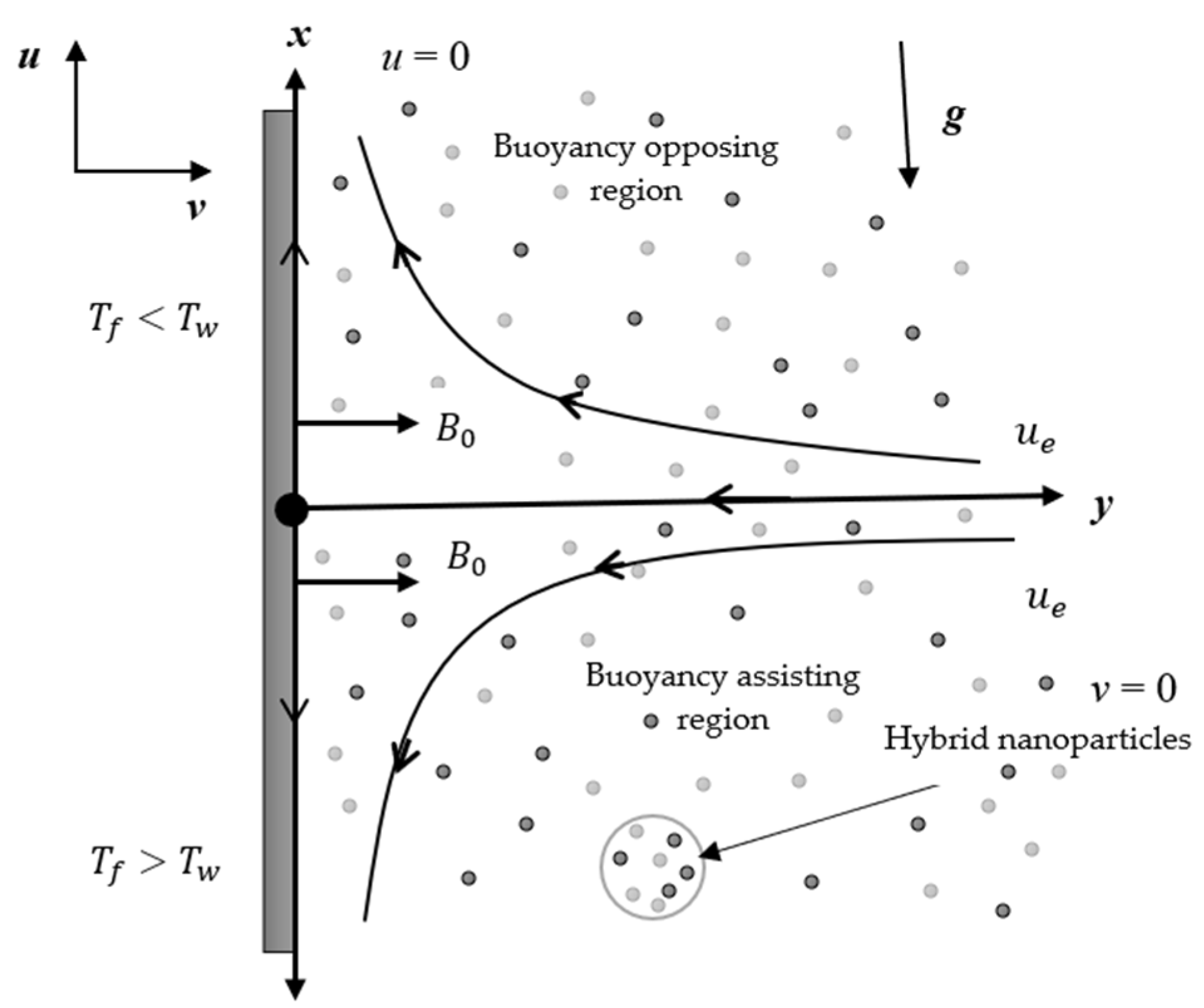
2. Formulation of the Mathematical Model

Consider the MHD flow of micropolar HNF along a vertically convective stretching/shrinking surface. x and y are the Cartesian coordinates, where the x-axis runs along the plate, and the y-axis is in the normal direction, the surface is laid down at $y=0$, and the flow is $y\ge 0$. It should be noted that mixed convection involves both opposing $\left(\lambda <0\right)$ and assisting $\left(\lambda >0\right)$ regions. The far flow (isothermal) velocity is $u_e\left(x\right)=ax$, where a is a positive constant, g is the acceleration due to gravity and the applied magnetic field, $B_0$ parallel to the y-axis, as shown in Figure 1. It is declared that the vertical plate is heated by the convection process because of the different temperatures between the fluid $T_f\left(x\right)$ and the ambient temperature $T_{\infty }\left(x\right)$, which produces a heat transfer coefficient $h_f\left(x\right)$.

Using the HNF model proposed by Takabi and Salehi [34], the governing conservation equations can be expressed as: [1,9,23,25,33]

$$\frac{\partial u}{\partial x}+\frac{\partial v}{\partial y}=0$$

(1)

$${\rho }_{Hnf}\left(u\frac{\partial u}{\partial x}+v\frac{\partial u}{\partial y}-u_e\frac{d{u}_e}{dx}\right)=\left({\mu }_{Hnf}+\kappa \right)\frac{{\partial }^{2}u}{\partial y^2}+\kappa \frac{\partial N}{\partial y}-{\sigma }_{Hnf}{B}_0{}^2\left(u-u_e\right)+{\left(\rho \beta \right)}_{Hnf}\left(T-T_{\infty }\right)g$$

(2)

$${\rho }_{Hnf}\left(u\frac{\partial N}{\partial x}+v\frac{\partial N}{\partial y}\right)=\frac{\chi }{j}\frac{{\partial }^{2}N}{\partial y^2}-\frac{\kappa }{j}\left(2N+\frac{\partial u}{\partial y}\right)$$

(3)

$${\left(\rho C_p\right)}_{Hnf}\left(u\frac{\partial T}{\partial x}+v\frac{\partial T}{\partial y}\right)=k_{Hnf}\frac{{\partial }^{2}T}{\partial y^2}$$

(4)

The BCs are

$$u=0,v=0,-k_{Hnf}\frac{\partial T}{\partial y}=h_f\left(T_f-T\right),N=-n\frac{\partial u}{\partial y} \mathrm{at} y=0$$

(5)

$$u\to u_e\left(x\right)=ax,N\to 0,T\to T_{\infty } \mathrm{as} y\to \infty$$

Here, u and v are the velocity components along the x and y axes, T, N, $\kappa$, $\chi$, g, $B_0$ is the temperature of the HNF, the microinertia density, vortex viscosity, spin gradient viscosity, acceleration due to gravity, and the coefficient of the magnetic field, respectively. n is a constant with n = 0 for the case of strong concentration, and it stipulates that N = 0 means that concentrated particle flows in such a way that the microelements near the surface cannot circulate. For the case, n = 1/2 signifies the dissipation of the anti-symmetric part of the stress tensor and indicates weak concentrations. While for the case, n = 1 is used for the turbulent boundary layer flow modeling.

Where ${\varphi }_1$ is the Al₂O₃ (alumina) and ${\varphi }_2$ is the Cu (copper) nanoparticle volume fraction, respectively. Besides that, $\rho$, $\mu$, $k$, $\left(\rho C_p\right)$, $\sigma$, and $\left(\rho \beta \right)$ are the densities, the dynamic viscosity, the thermal conductivities, the heat capacitance, the electrical conductivity, and the thermal expansion, respectively. For clarity, subscripts f, nf, and Hnf represent the base fluid, the nanofluid, and HNF, respectively, as shown in

Table 1. Thermophysical correlations of Al₂O_3–Cu/H₂O (see [35,36,37]).

Properties	Nanofluid	Hybrid Nanofluid
Density	${\rho }_{nf}=\left(1-{\varphi }_1\right){\rho }_f+{\varphi }_2{\rho }_{n1}$	${\rho }_{Hnf}=\left(1-{\varphi }_2\right)\left[\left(1-{\varphi }_1\right){\rho }_f+{\varphi }_1{\rho }_{n1}\right]+{\varphi }_2{\rho }_{n2}$
Dynamic viscosity	${\mu }_{nf}=\frac{{\mu }_f}{{\left(1-{\varphi }_1\right)}^{5/2}}$	${\mu }_{Hnf}=\frac{{\mu }_f}{{\left(1-{\varphi }_1\right)}^{5/2}{\left(1-{\varphi }_2\right)}^{5/2}}$
Thermal conductivity	$\frac{k_{nf}}{k_f}=\frac{k_{n1}+2k_f-2{\varphi }_1\left(k_f-k_{n1}\right)}{k_{n1}+2k_f+{\varphi }_1\left(k_f-k_{n1}\right)}$	$\begin{array}{l}\frac{k_{Hnf}}{k_{nf}}=\frac{k_{n2}+2k_{nf}-2{\varphi }_2\left(k_{nf}-k_{n2}\right)}{k_{n2}+2k_{nf}+{\varphi }_2\left(k_{nf}-k_{n2}\right)}\\ \frac{k_{nf}}{k_f}=\frac{k_{n1}+2k_f-2{\varphi }_1\left(k_f-k_{n1}\right)}{k_{n1}+2k_f+{\varphi }_1\left(k_f-k_{n1}\right)} \end{array}$ where
Electrical conductivity	$\frac{{\sigma }_{nf}}{{\sigma }_f}=\frac{{\sigma }_{n1}+2{\sigma }_f-2{\varphi }_1\left({\sigma }_f-{\sigma }_{n1}\right)}{{\sigma }_{n1}+2{\sigma }_f+{\varphi }_1\left({\sigma }_f-{\sigma }_{n1}\right)}$	$\begin{array}{l}\frac{{\sigma }_{Hnf}}{{\sigma }_{nf}}=\frac{{\sigma }_{n2}+2{\sigma }_{nf}-2{\varphi }_2\left({\sigma }_{nf}-{\sigma }_{n2}\right)}{{\sigma }_{n2}+2{\sigma }_{nf}+{\varphi }_2\left({\sigma }_{nf}-{\sigma }_{n2}\right)}\\ \frac{{\sigma }_{nf}}{{\sigma }_f}=\frac{{\sigma }_{n1}+2{\sigma }_f-2{\varphi }_1\left({\sigma }_f-{\sigma }_{n1}\right)}{{\sigma }_{n1}+2{\sigma }_f+{\varphi }_1\left({\sigma }_f-{\sigma }_{n1}\right)} \end{array}$ where
Heat capacity	${\left(\rho C_p\right)}_{nf}=\left(1-{\varphi }_2\right){\left(\rho C_p\right)}_f+{\varphi }_1{\left(\rho C_p\right)}_{n1}$	${\left(\rho C_p\right)}_{Hnf}=\left(1-{\varphi }_2\right)\left[\left(1-{\varphi }_1\right){\left(\rho C_p\right)}_f+{\varphi }_1{\left(\rho C_p\right)}_{n1}\right]+{\varphi }_2{\left(\rho C_p\right)}_{n2}$
Thermal expansion	${\left(\rho \beta \right)}_{nf}=\left(1-{\varphi }_2\right){\left(\rho \beta \right)}_f+{\varphi }_1{\left(\rho \beta \right)}_{n1}$	${\left(\rho \beta \right)}_{Hnf}=\left(1-{\varphi }_2\right)\left[\left(1-{\varphi }_1\right){\left(\rho \beta \right)}_f+{\varphi }_1{\left(\rho \beta \right)}_{n1}\right]+{\varphi }_2{\left(\rho \beta \right)}_{n2}$

.

Table 2. Thermophysical properties (see [38]).

Physical Properties	Al2O3	Cu	Water
Prandtl number, Pr			6.2
$\beta \times {10}^{-5}\left(\frac{1}{K}\right)$	0.85	1.67	21
$k\left(\frac{W}{mK}\right)$	40	400	0.613
$C_p\left(\frac{J}{KgK}\right)$	765	385	4179
$\sigma \left(\frac{S}{m}\right)$	$3.69\times {10}^7$	$5.96\times {10}^7$	0.05
$\rho \left(\frac{kg}{m^3}\right)$	3970	8933	997.1

provides the values of the thermophysical properties of the nanoparticles and water (base fluid).

It is understood that $\chi =\left({\mu }_{Hnf}+\kappa /2\right)$ and $j={\nu }_f/a$, where $K=\kappa /{\mu }_f$ is the material parameter and L is the surface characteristic length, respectively. For the fluid temperature $T_f\left(x\right)=T_{\infty }+T_0\left(x/L\right)$, $T_0$ is the surface temperature characteristic with $T_0>0$, $T_0<0$ and $T_0=0$ are for assisting, opposing and forced convection flow, respectively.

According to Ul Haq et al. [9], the following dimensionless variables are circumscribed as

$$\begin{array}{l}\psi \left(x,y\right)=\sqrt{a{\nu }_f}xf\left(\eta \right),\hspace{1em}N\left(x,y\right)=ax\sqrt{a/{\nu }_f}h\left(\eta \right),\\ \theta \left(\eta \right)=\left(T-T_{\infty }\right)/\left(T_f-T_{\infty }\right),\hspace{1em}\eta =y\sqrt{a/{\nu }_f}\end{array}$$

(6)

where $\psi$ is the stream function, defined as $u=\frac{\partial \psi }{\partial y}$ and $v=\frac{-\partial \psi }{\partial x}$. By employing the similarity variables (7), Equations (2) to (4) are reduced to the following ODEs:

$$\frac{1}{{\rho }_{HF}}\left({\mu }_{HF}+{\rm K}\right)f^{‴}+f{f}^{″}+1-{f^{\prime }}^2+\frac{1}{{\rho }_{HF}}{\rm K}{h}^{\prime }-\frac{{\sigma }_{HF}}{{\rho }_{HF}}{M}^2\left(f^{\prime }-1\right)+\frac{{\left(\rho \beta \right)}_{HF}}{{\rho }_{HF}}\lambda \theta =0$$

(7)

$$\frac{1}{{\rho }_{HF}}\left({\mu }_{HF}+\frac{{\rm K}}{2}\right)h^{″}+f{h}^{\prime }-f^{\prime } h-\frac{{\rm K}}{{\rho }_{HF}}\left(2h+f^{″}\right)=0$$

(8)

$$\frac{1}{\mathrm{Pr}}\frac{k_{HF}}{{\left(\rho C_p\right)}_{HF}}{\theta }^{″}+f{\theta }^{\prime }-f^{\prime }\theta =0$$

(9)

$$f\left(0\right)=0,\hspace{1em}{f}^{\prime }\left(0\right)=0, h\left(0\right)=-n{f}^{″}\left(0\right),\hspace{1em}-k_{HF}{\theta }^{\prime }\left(0\right)=Bi\left[1-\theta \left(0\right)\right]$$

(10)

$$f^{\prime }\left(\eta \right)\to 1,\hspace{1em}h\left(\eta \right)\to 0,\hspace{1em}\theta \left(\eta \right)\to 0 \mathrm{as} \eta \to \infty$$

where

$$\begin{array}{c}{\mu }_{HF}=\frac{{\mu }_{Hnf}}{{\mu }_f},\hspace{1em}{\rho }_{HF}=\frac{{\rho }_{Hnf}}{{\rho }_f},\hspace{1em}{\sigma }_{HF}=\frac{{\sigma }_{Hnf}}{{\sigma }_f},\hspace{1em}{k}_{HF}=\frac{k_{Hnf}}{k_f},\\ {\left(\rho C_p\right)}_{HF}=\frac{{\left(\rho C_p\right)}_{Hnf}}{{\left(\rho C_p\right)}_f},\hspace{1em}{\left(\rho \beta \right)}_{HF}=\frac{{\left(\rho \beta \right)}_{Hnf}}{{\left(\rho \beta \right)}_f}\end{array}$$

(11)

Here, primes represent differentiation with respect to $\eta$, $M$ is the magnetic parameter, $\mathrm{Pr}$ is the Prandtl number, $Bi$ is the Biot number, and $\lambda$ is the constant mixed convection parameter, which is defined as

$$M=\sqrt{\frac{{\sigma }_f{\beta }_0{}^2}{{\rho }_{f}a}},\hspace{1em}\mathrm{Pr}=\frac{{\nu }_f}{{\alpha }_f},\hspace{1em}Bi=\frac{h_f}{k_f}\sqrt{\frac{{\nu }_f}{a}},\hspace{1em}\lambda =\frac{G{r}_x}{{\mathrm{Re}}_x{}^2}$$

(12)

with the local Grashof number,$G{r}_x=g{\beta }_f\left(T_f-T_{\infty }\right)x^3/{\nu }_f{}^2$, and the local Reynolds number, ${\mathrm{Re}}_x=u_{e}x/{\nu }_f$.

The quantities of physical interest are the skin friction coefficient $C_f$, local couple stress $M_x$, and the local Nusselt number $N{u}_x$, which are defined as ([1,13]);

$$\begin{array}{l}{C}_f=\frac{1}{{\rho }_f{u}_e{}^2}{\left(\left({\mu }_{Hnf}+\kappa \right)\frac{\partial u}{\partial y}+\kappa N\right)}_{y=0},\hspace{1em}{M}_x=\frac{\chi }{{\rho }_{f}x{u}_e{}^2}{\left(\frac{\partial N}{\partial y}\right)}_{y=0},\\ N{u}_x=\frac{x{k}_{Hnf}}{k_f\left(T_f-T_{\infty }\right)}{\left(-\frac{\partial T}{\partial y}\right)}_{y=0}\end{array}$$

(13)

Using (6) and (13), we get

$$\begin{array}{l}{\mathrm{Re}}_x{}^{1/2}{C}_f=\left({\mu }_{HF}+K\left(1-n\right)\right)f^{″}\left(0\right),\hspace{1em}{\mathrm{Re}}_x{M}_x=\left({\mu }_{HF}+\frac{K}{2}\right)h^{\prime }\left(0\right),\\ \frac{N{u}_x}{{\mathrm{Re}}_x{}^{1/2}}=-k_{HF}{\theta }^{\prime }\left(0\right)\end{array}$$

(14)

3. Temporal Stability Analysis

Many problems have proven that the stability inquiry for the first branch is physically stable or acceptable. However, a problem exists where the first solution is unstable, as reported by Anuar et al. [25]. Thus, it is practical to perform this temporal stability inquiry and verify the reliability of the outcome(s). Physically, if there exists a disturbance (perturbation) for initial growth in the solution, the outcome is not real. However, the disturbance or perturbation may decay or increase exponentially over time. This is why an unsteady problem is considered. Following Weidman et al. [39] and Merkin [40], an unsteady form of Equations (2)–(4) are

$$\begin{array}{l}\frac{\partial u}{\partial t}+u\frac{\partial u}{\partial x}+v\frac{\partial u}{\partial y}-u_e\frac{d{u}_e}{dx}=\frac{\left({\mu }_{Hnf}+\kappa \right)}{{\rho }_{Hnf}}\frac{{\partial }^{2}u}{\partial y^2}+\frac{\kappa }{{\rho }_{Hnf}}\frac{\partial N}{\partial y}-\frac{{\sigma }_{Hnf}}{{\rho }_{Hnf}}{B}_0{}^2\left(u-u_e\right)\\ +\frac{{\left(\rho \beta \right)}_{Hnf}}{{\rho }_{Hnf}}\left(T-T_{\infty }\right)g\end{array}$$

(15)

$$\frac{\partial N}{\partial t}+u\frac{\partial N}{\partial x}+v\frac{\partial N}{\partial y}=\frac{\chi }{{\rho }_{Hnf}}\frac{{\partial }^{2}N}{\partial y^2}-\frac{\kappa }{{\rho }_{Hnf}}\left(2N+\frac{\partial u}{\partial y}\right)$$

(16)

$$\frac{\partial T}{\partial t}+u\frac{\partial T}{\partial x}+v\frac{\partial T}{\partial y}=\frac{k_{Hnf}}{{\left(\rho C_p\right)}_{Hnf}}\frac{{\partial }^{2}T}{\partial y^2}$$

(17)

The relevant similarity transformation for the unsteady problem is given by

$$\begin{array}{c}\eta =y\sqrt{a/{\nu }_f},\hspace{1em}\psi =\sqrt{a{\nu }_f}xf\left(\eta ,\tau \right),\hspace{1em}N=ax\sqrt{a/{\nu }_f}h\left(\eta ,\tau \right),\\ \theta \left(\eta ,\tau \right)=\left(T-T_{\infty }\right)/\left(T_f-T_{\infty }\right),\hspace{1em}\tau =at\end{array}$$

(18)

Using (18), Equations (15)–(17) can be rewritten as

$$\begin{array}{l}\frac{\left({\mu }_{HF}+K\right)}{{\rho }_{HF}}\frac{{\partial }^{3}f}{\partial {\eta }^3}\left(\eta ,\tau \right)+f\left(\eta ,\tau \right)\frac{{\partial }^{2}f}{\partial {\eta }^2}\left(\eta ,\tau \right)-{\left(\frac{\partial f}{\partial \eta }\left(\eta ,\tau \right)\right)}^2-\frac{{\partial }^{2}f}{\partial \tau \partial \eta }\left(\eta ,\tau \right)+1\\ +\frac{K}{{\rho }_{HF}}\frac{\partial h}{\partial \eta }\left(\eta ,\tau \right)-\frac{{\sigma }_{HF}}{{\rho }_{HF}}{M}^2\left(\frac{\partial f}{\partial \eta }\left(\eta ,\tau \right)-1\right)+\frac{{\left(\rho \beta \right)}_{HF}}{{\rho }_{HF}}\lambda \theta \left(\eta ,\tau \right)=0\end{array}$$

(19)

$$\begin{array}{l}\frac{1}{{\rho }_{HF}}\left({\mu }_{HF}+\frac{K}{2}\right)\frac{{\partial }^{2}h}{\partial {\eta }^2}\left(\eta ,\tau \right)-\frac{\partial f}{\partial \eta }\left(\eta ,\tau \right)h\left(\eta ,\tau \right)+f\left(\eta ,\tau \right)\frac{\partial h}{\partial \eta }\left(\eta ,\tau \right)-\frac{\partial h}{\partial \tau }\left(\eta ,\tau \right)\\ -\frac{K}{{\rho }_{HF}}\left(2h\left(\eta ,\tau \right)+\frac{{\partial }^{2}f}{\partial {\eta }^2}\left(\eta ,\tau \right)\right)=0\end{array}$$

(20)

$$\frac{1}{\mathrm{Pr}}\frac{k_{HF}}{{\left(\rho C_p\right)}_{HF}}\frac{{\partial }^2\theta }{\partial {\eta }^2}\left(\eta ,\tau \right)-\frac{\partial f}{\partial \eta }\left(\eta ,\tau \right)\theta \left(\eta ,\tau \right)+f\left(\eta ,\tau \right)\frac{\partial \theta }{\partial \eta }\left(\eta ,\tau \right)-\frac{\partial \theta }{\partial \tau }\left(\eta ,\tau \right)=0$$

(21)

The conditions are

$$\begin{array}{l}f\left(0,\tau \right)=0,\hspace{1em}\frac{\partial f}{\partial \eta }\left(0,\tau \right)=0,\hspace{1em}h\left(0,\tau \right)=-n\frac{{\partial }^{2}f}{\partial {\eta }^2}\left(0,\tau \right),\hspace{1em}-k_{HF}\frac{\partial \theta }{\partial \eta }\left(0,\tau \right)=Bi\left(1-\theta \left(0,\tau \right)\right),\\ \frac{\partial f}{\partial \eta }\left(\eta ,\tau \right)\to 1,\hspace{1em}h\left(\eta ,\tau \right)\to 0,\hspace{1em}\theta \left(\eta ,\tau \right)\to 0,\hspace{1em} \mathrm{as} \eta \to \infty \end{array}$$

(22)

$$\begin{gathered} f\left(\eta ,\tau \right)=f_1\left(\eta \right)+e^{-\gamma \tau }{F}_1\left(\eta \right),H\left(\eta ,\tau \right)=h_1\left(\eta \right)+e^{-\gamma \tau }{H}_1\left(\eta \right) \mathrm{and} \\ \theta \left(\eta ,\tau \right)={\theta }_1\left(\eta \right)+e^{-\gamma \tau }{G}_1\left(\eta \right) \end{gathered}$$

(23)

which are the perturbation equations introduced to determine and verify the temporal stability, following Weidman et al. [41]. $\gamma$ is an unknown eigenvalue parameter whereas $f\left(\eta \right)=f_1\left(\eta \right), h\left(\eta \right)=h_1\left(\eta \right), \theta \left(\eta \right)={\theta }_1\left(\eta \right)$ are the steady state solutions; $F_1\left(\eta \right)$, $H_1\left(\eta \right)$ and $G_1\left(\eta \right)$ are a small relative to $f_1\left(\eta \right)$, $h_1\left(\eta \right)$ and ${\theta }_1\left(\eta \right)$, respectively. Substituting Equation (23) into Equations (19) to (22), we obtain

$$\begin{array}{l}\frac{\left({\mu }_{HF}+K\right)}{{\rho }_{HF}}{F^{‴}}_1\left(\eta \right)+f_1{}^{″}\left(\eta \right)F_1\left(\eta \right)+f_1\left(\eta \right){F^{″}}_1\left(\eta \right)+\left(\gamma -2f_1{}^{\prime }\left(\eta \right)\right){F^{\prime }}_1\left(\eta \right)+\frac{K}{{\rho }_{HF}}{H^{\prime }}_1\left(\eta \right)\\ -\frac{{\sigma }_{HF}}{{\rho }_{HF}}{M}^2{F^{\prime }}_1\left(\eta \right)+\frac{{\left(\rho \beta \right)}_{HF}}{{\rho }_{HF}}\lambda G_1\left(\eta \right)=0\end{array}$$

(24)

$$\begin{array}{l}\frac{1}{{\rho }_{HF}}\left({\mu }_{HF}+\frac{K}{2}\right){H^{″}}_1\left(\eta \right)-h_1\left(\eta \right){F^{\prime }}_1\left(\eta \right)+\left(\gamma -f_1{}^{\prime }\left(\eta \right)\right)H_1\left(\eta \right)+h_1{}^{\prime }{F}_1\left(\eta \right)+f_1\left(\eta \right){H^{\prime }}_1\left(\eta \right)\\ -\frac{K}{{\rho }_{HF}}\left(2H_1\left(\eta \right)+{F^{″}}_1\left(\eta \right)\right)=0\end{array}$$

(25)

$$\frac{1}{\mathrm{Pr}}\frac{k_{HF}}{{\left(\rho C_p\right)}_{HF}}{G^{″}}_1\left(\eta \right)-{\theta }_1\left(\eta \right){F^{\prime }}_1\left(\eta \right)+\left(\gamma -{f^{\prime }}_1\left(\eta \right)\right)G_1\left(\eta \right)+{{\theta }^{\prime }}_1\left(\eta \right)F_1\left(\eta \right)+f_1\left(\eta \right){G^{\prime }}_1\left(\eta \right)=0$$

(26)

with the conditions

$$\begin{array}{l}{F}_1\left(0\right)=0,\hspace{1em}{F^{\prime }}_1\left(0\right)=0,\hspace{1em}{H}_1\left(0\right)=-n{F}^{″}\left(0\right),\hspace{1em}{G^{\prime }}_1\left(0\right)=\frac{1}{k_{HF}}Bi{G}_1\left(0\right),\\ {F^{\prime }}_1\left(\eta \right)\to 0,\hspace{1em}{H}_1\left(\eta \right)\to 0,\hspace{1em}{G}_1\left(\eta \right)\to 0 \mathrm{as} \eta \to \infty \end{array}$$

(27)

To determine the stability of the solution, Equations (24) to (27) are solved using the bvp4c solver. Equation (27) is relaxed as the derivative ${F^{\prime }}_1\left(\eta \right)\to 0, \eta \to \infty$ and substituted with the new BC, which is ${F^{″}}_1\left(0\right)=1$. This replacement is performed to obtain the smallest eigenvalue, as mentioned by Harris et al. [42].

4. Result and Discussion

The similarity Equations (6) and (7) are solved numerically using the bvp4c solver in the MATLAB software with respect to BC Equation (8). This bvp4c solver is introduced by Shampine et al. [43], which implements the 3-stage Lobatto IIIa finite difference method, which provides fourth-order accuracy uniformly in the interval where the function is integrated, known as the collocation formula. To initiate the bvp4c solver, the nonlinear ODEs should be first reduced to a first-order system before it is solved. In this solving approach, the appropriate guess for the initial values and the boundary layer thickness ${\eta }_{\infty }$ is important to obtain the correct numerical solutions for the present problem. Since the current problem has a dual solution, the bvp4c function requires an initial guess, which should satisfy the boundary conditions and reveals the behavior of the desired solution. It is easy to find the initial guess for the first solution because the bvp4c will eventually converge to the first solution, even if we are using poor guesses. However, the initial guess for the second solution is quite challenging. Several values are considered in this study, such as material parameter K, mixed convection parameter λ, magnetic parameter M, Biot number Bi and the nanoparticles volume fraction ϕ₁, ϕ₂, and we assume for only the case n = 0.5 (weak concentration) throughout this study, to save space. Our results the $f^{″}\left(0\right)$ and $-{\theta }^{\prime }\left(0\right)$ are verified to those of the previous researcher, Khashi’ie et al. [44], for assisting flow $\lambda =1$, excluding hybrid nanoparticles ϕ₁ = ϕ₂ = 0, material parameter K = 0, magnetic parameter M = 0 and Biot number $Bi=\infty$ for different values of Pr, and they demonstrate excellent agreement as displayed in

Table 3. Comparison values of $f^{″}\left(0\right)$ and $-{\theta }^{\prime }\left(0\right)$ for distinct values of Pr.

Pr	${\mathit{f}}^{″}\left(0\right)$				$-{\mathit{\theta }}^{\prime }\left(0\right)$
	Khashi’ie et al. [44]		Result		Khashi’ie et al. [44]		Result
	First Solution	Second Solution	First Solution	Second Solution	First Solution	Second Solution	First Solution	Second Solution
0.7	1.7063	1.2387	1.70632265	1.23872774	0.7641	1.0226	0.76406346	1.02263139
1.0	1.6754	1.1332	1.67543657	1.13319247	0.8708	1.1691	0.87077860	1.16912606
7.0	1.5179	0.5824	1.51791262	0.58240096	1.7224	2.2191	1.72238160	2.21919411
10.0	1.4928	0.4958	1.49283867	0.49577941	1.9446	2.4940	1.94461739	2.49402854
20.0	1.4485	0.3436	1.44848293	0.34364027	2.4576	3.1646	2.45759005	3.16460845
25.0	-	-	1.43546650	0.29898184	-	-	2.64901124	3.43169660
30.0	-	-	1.42528871	0.26393460	-	-	2.81614709	3.67382853
35.0	-	-	1.41700206	0.23526178	-	-	2.96547712	3.89784204

. The analysis proves that the results of the current research are reliable and consistent. Furthermore,

Table 4. Values of Re_x^1/2 C_f, Re_x M_x, and Re_x^−1/2 Nu_x when Pr = 6.2, Bi = 0.5, and n = 0.5.

${\mathit{\varphi }}_{\mathit{H}\mathit{n}\mathit{f}}(\%)$	K	M	Buoyancy Assisting Flow (λ = 1)			Buoyancy Opposing Flow (λ = −1)
			Rex1/2 Cf	Rex Mx	Rex−1/2 Nux	Rex1/2 Cf	Rex Mx	Rex−1/2 Nux
0	1	1	1.97922464	0.76391084	0.38057597	1.84976934	0.68708906	0.37910938
1			2.0172647	0.80745604	0.38320124	1.89246669	0.73150002	0.38183689
2	0		1.71224371	0.77248271	0.39006488	1.59709875	0.71213373	0.38870291
	1		2.06065407	0.82753810	0.38487081	1.93793993	0.75293929	0.38357284
	2		2.37147874	0.85861598	0.38110822	2.23798198	0.77586364	0.37983740
	3		2.64941168	0.88067491	0.37811387	2.50565957	0.79194192	0.37686108
	1	0	1.66276884	0.59712546	0.37962477	1.51439939	0.51082685	0.37762116
		1	2.06065407	0.82753810	0.38487081	1.93793993	0.75293929	0.38357284
		2	2.92254421	1.36368321	0.39289368	2.83216499	1.30502064	0.3922474
		3	3.93032828	2.03436344	0.39910432	3.86075439	1.98690311	0.39874551
4	1	1	2.13961467	0.89160541	0.38893447	2.02308939	0.81910872	0.38778014

presents the output values of difference parameters on Re_x^1/2 C_f, Re_x M_x, and Re_x^−1/2 Nu_x for both buoyancy assisting and opposing flow $\left(\lambda =\pm 1\right)$. For both buoyancy flows, the physical quantities values Re_x^1/2 C_f, Re_x M_x, and Re_x^−1/2 Nu_x are increased as ${\varphi }_{Hnf}$, K, and M increase. However, the values are decreased only for Re_x^−1/2 Nu_x when K is raised.

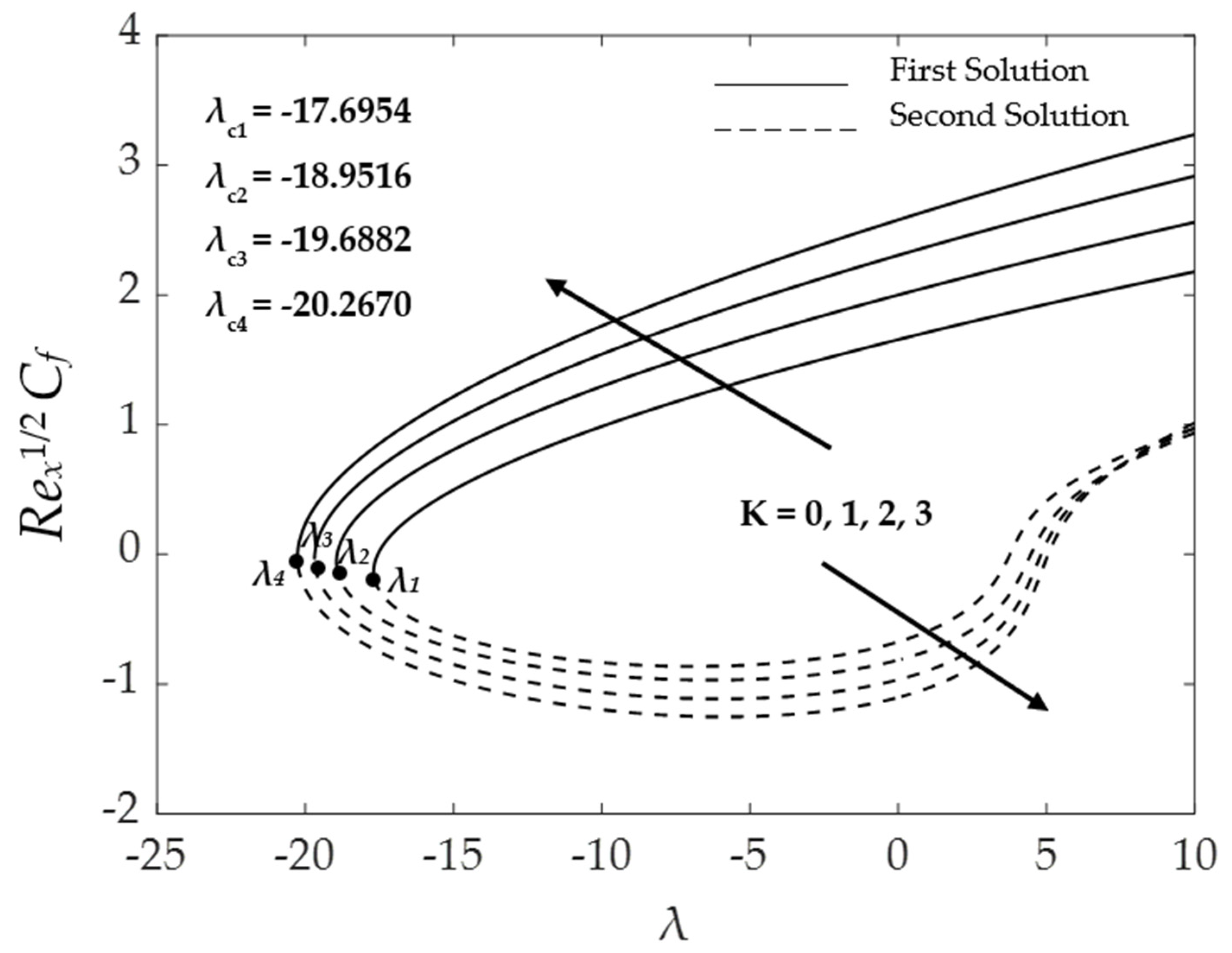
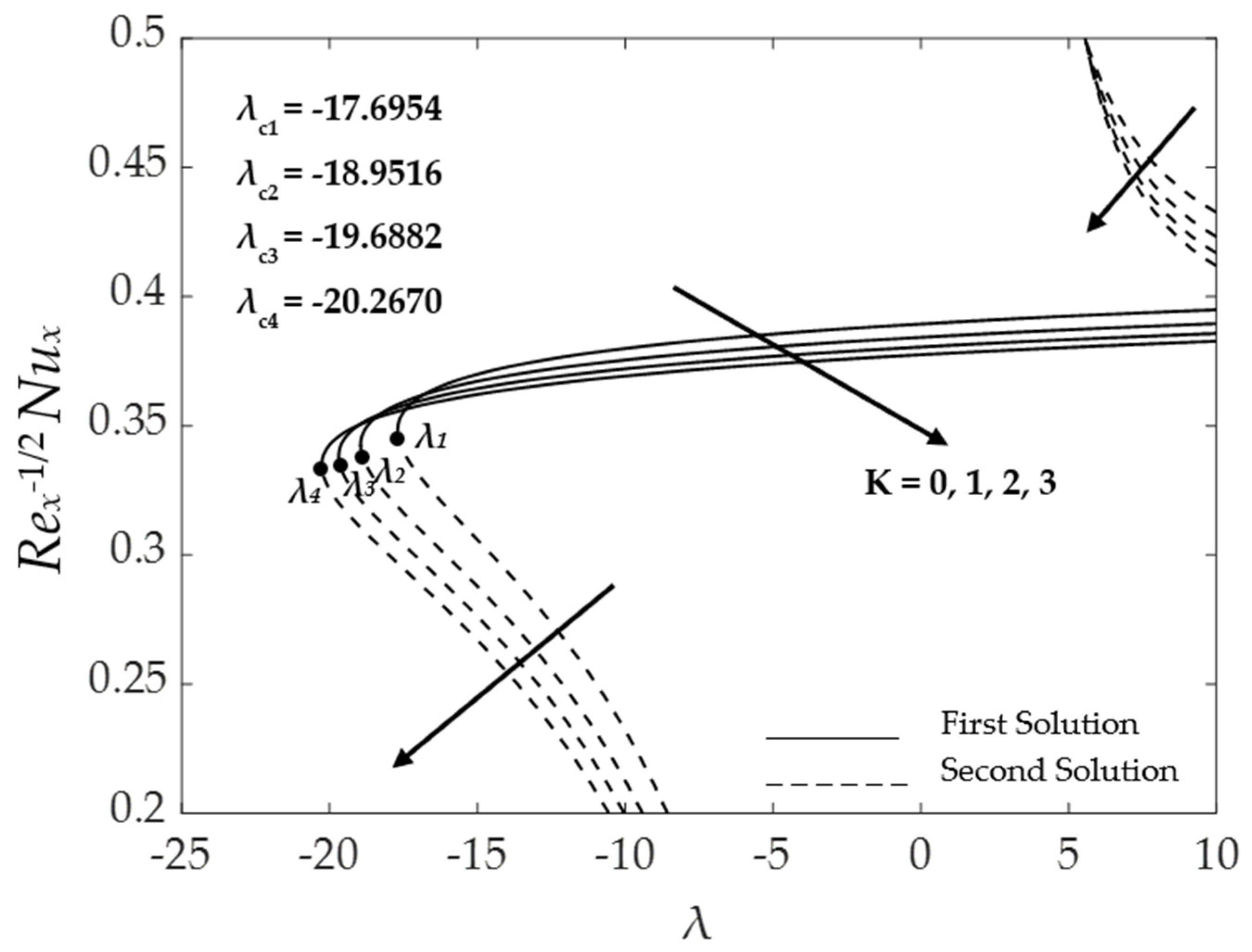
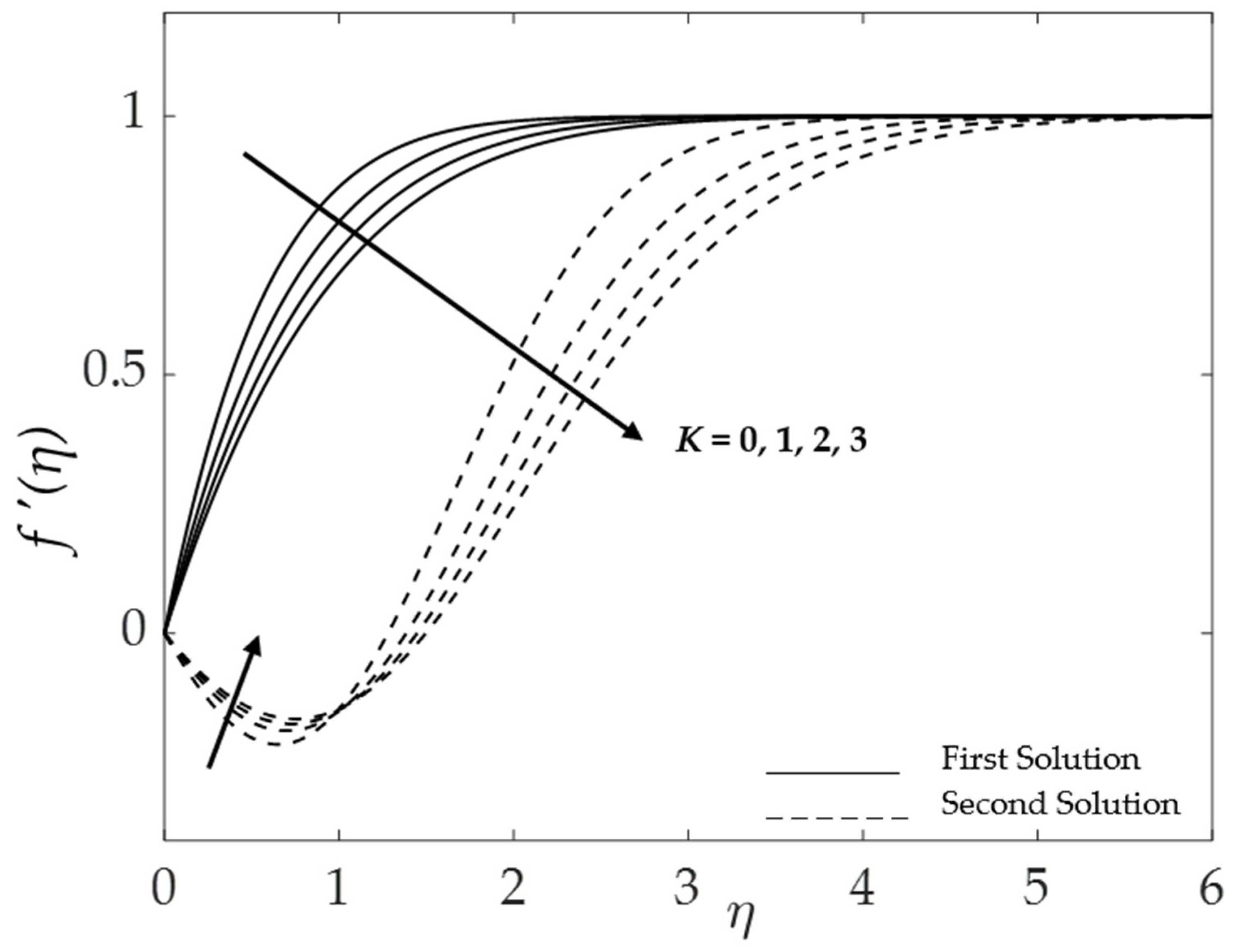
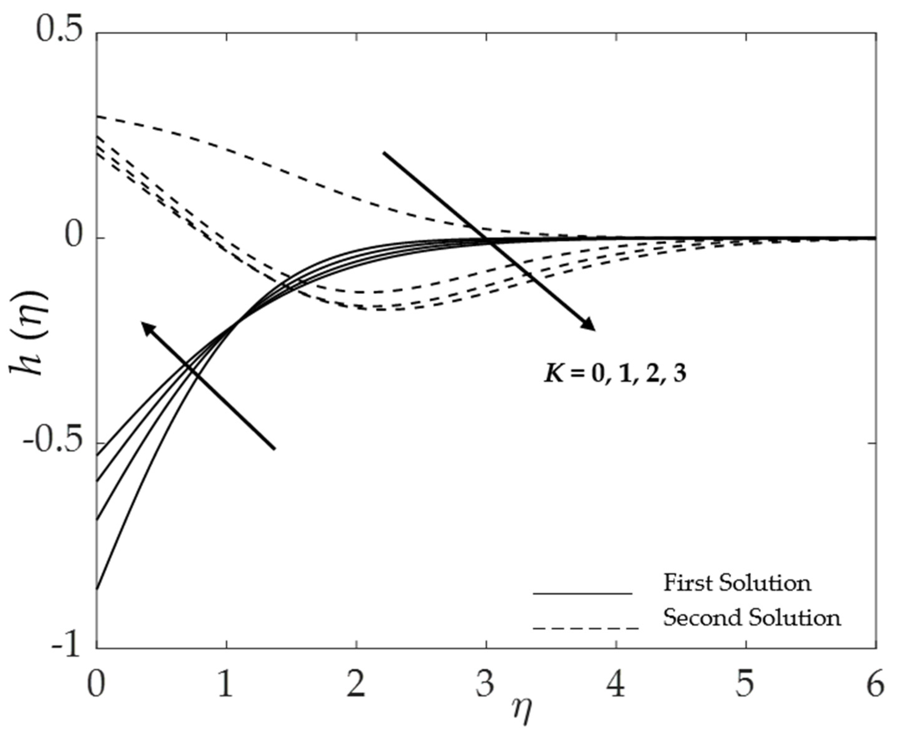
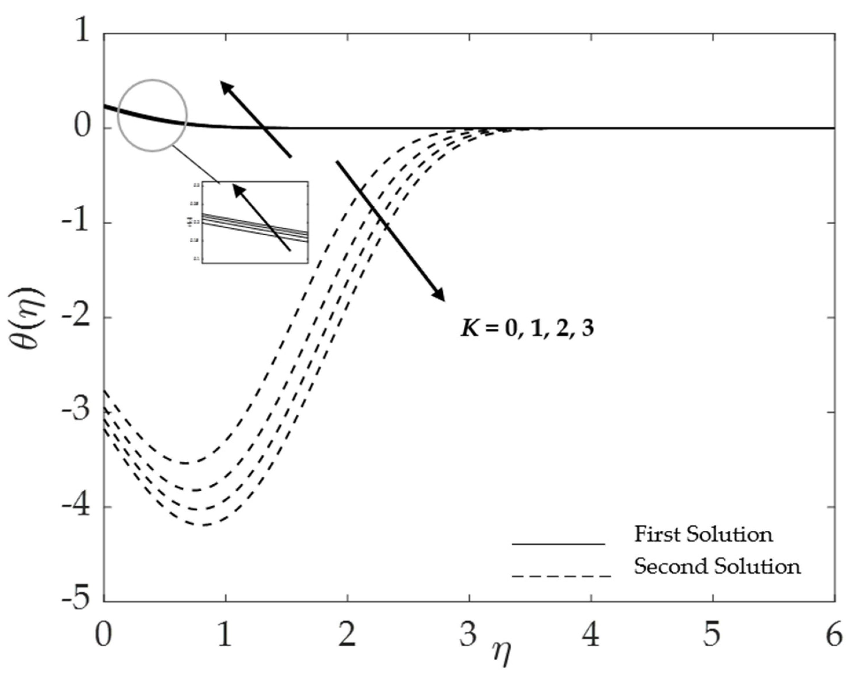
4.1. Effect of the Material Parameter $\left(K\right)$

Figure 2 and Figure 3 illustrate the differences of ${\mathit{Re}}_x{}^{1/2}{C}_f$ and ${\mathit{Re}}_x{}^{-1/2}N{u}_x$ for some values of $K$ when $M=1$, $\mathrm{Pr}=6.2$, $Bi=n=0.5$ and ${\varphi }_1={\varphi }_2=1\%$. These figures show that it is possible to obtain double outcomes of the similarity Equations (7) to (9) for both assisting and opposing flows, $\lambda =\pm 1$. Due to buoyancy forces, $\lambda >0$ experiences a favorable pressure gradient, which accelerates the flow and causes a larger skin friction coefficient than in the non-buoyant scenario $\lambda =0$. The unique solution $\lambda ={\lambda }_c$ (negative values of $\lambda$) and double outcomes in the range $\lambda >{\lambda }_c$ exist, but there is no outcome for $\lambda <{\lambda }_c$. The boundary layer separates from the surface at $\lambda ={\lambda }_c$; thus, we are unable to get the solution beyond this value. Based on the computations, ${\lambda }_{c1}=-17.6954$, ${\lambda }_{c2}=-18.9516$, ${\lambda }_{c3}=-19.6882$, and ${\lambda }_{c4}=-20.2670$ for K = 0, 1, 2, 3, respectively. Moreover, for both assisting and opposing cases, ${\mathit{Re}}_x{}^{1/2}{C}_f$ rises with rising K for the first solution, but it declines for the second solution, respectively, as shown in Figure 2. It is noted that the rise of ${\mathit{Re}}_x{}^{1/2}{C}_f$ is due to the existence of material parameter compared to K = 0 (absence of material parameter). Since micropolar fluid (MF) consists of rigid, randomly oriented, or spherical particles that are suspended in a viscous fluid, they have their own microrotations and spins. This suggests that MFs have a high resistance to fluid motion. Furthermore, according to this approach, the largest material parameter value will increase the vortex viscosity of the fluid flow. As a result, the MF is a very effective means of controlling the laminar boundary layer flow. Figure 3 depicts the heat transfer rate (HTR) at the surface of ${\mathit{Re}}_x{}^{-1/2}N{u}_x$, which decreases as the material parameter, K, increases. This is due to the increasing rate of vortex viscosity, which result in an upsurge in the friction at the surface and hence decrease the HTR at the wall. This discovery is consistent with earlier research performed by Anuar and Bachok [25].

Next, the effects of the material parameter K on the velocity $f^{\prime }\left(\eta \right)$, microrotation $h\left(\eta \right)$, and temperature profiles $\theta \left(\eta \right)$ when M = 1, Bi = n = 0.5, ϕ₁ = ϕ₂ = 0.01, and λ = 1 are illustrated in Figure 4, Figure 5 and Figure 6. It is noticed that the velocity and microrotation profiles decrease by increasing the micropolar effects for both solutions. However, for the velocity profile $f^{\prime }\left(\eta \right)$, the profile increases for the range of $\left(0\le \eta \le 1\right)$ for the second solution and then monotonically decreases for the range $\left(\eta \ge 1\right)$, as depicted in Figure 4. Figure 5 represents a similar pattern to Figure 4, but the profile increases in the beginning for the range $\left(0\le \eta \le 1.2\right)$ for the first solution and then monotonically decreases for the range $\left(\eta \ge 1.2\right)$. In addition, the rise of K leads the momentum boundary layer thickness to increase because of the dynamic viscosities that take place, as well as the vortex effects. Nonetheless, the temperature profiles present the opposite behaviors, as shown in Figure 6. The temperature escalates for the first solution and reduces for the second solution when K is increasing. This discovery is also consistent with those of Waini et al. [24] for velocity and temperature profiles, but for the microrotation profiles, the results are in contrast.

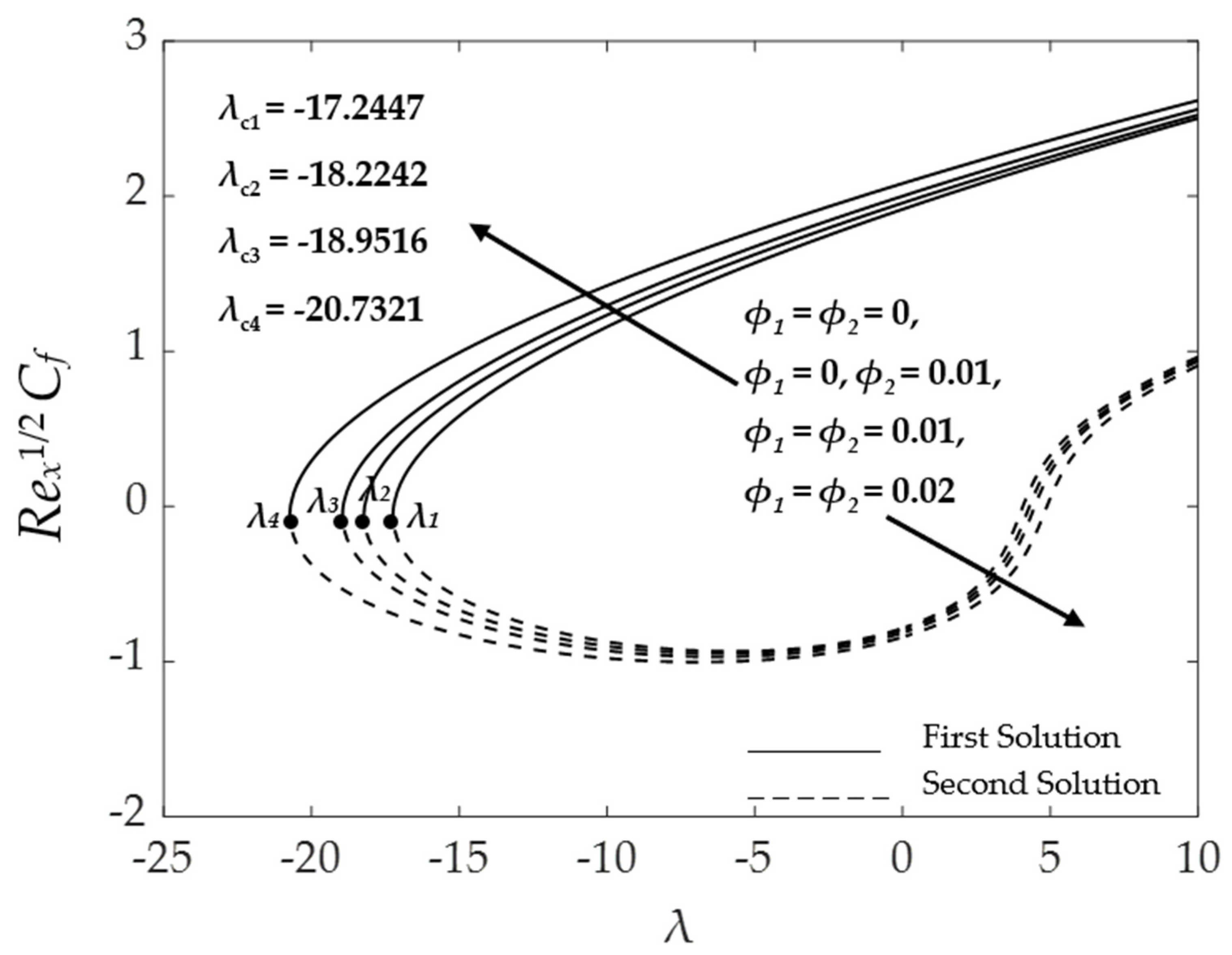
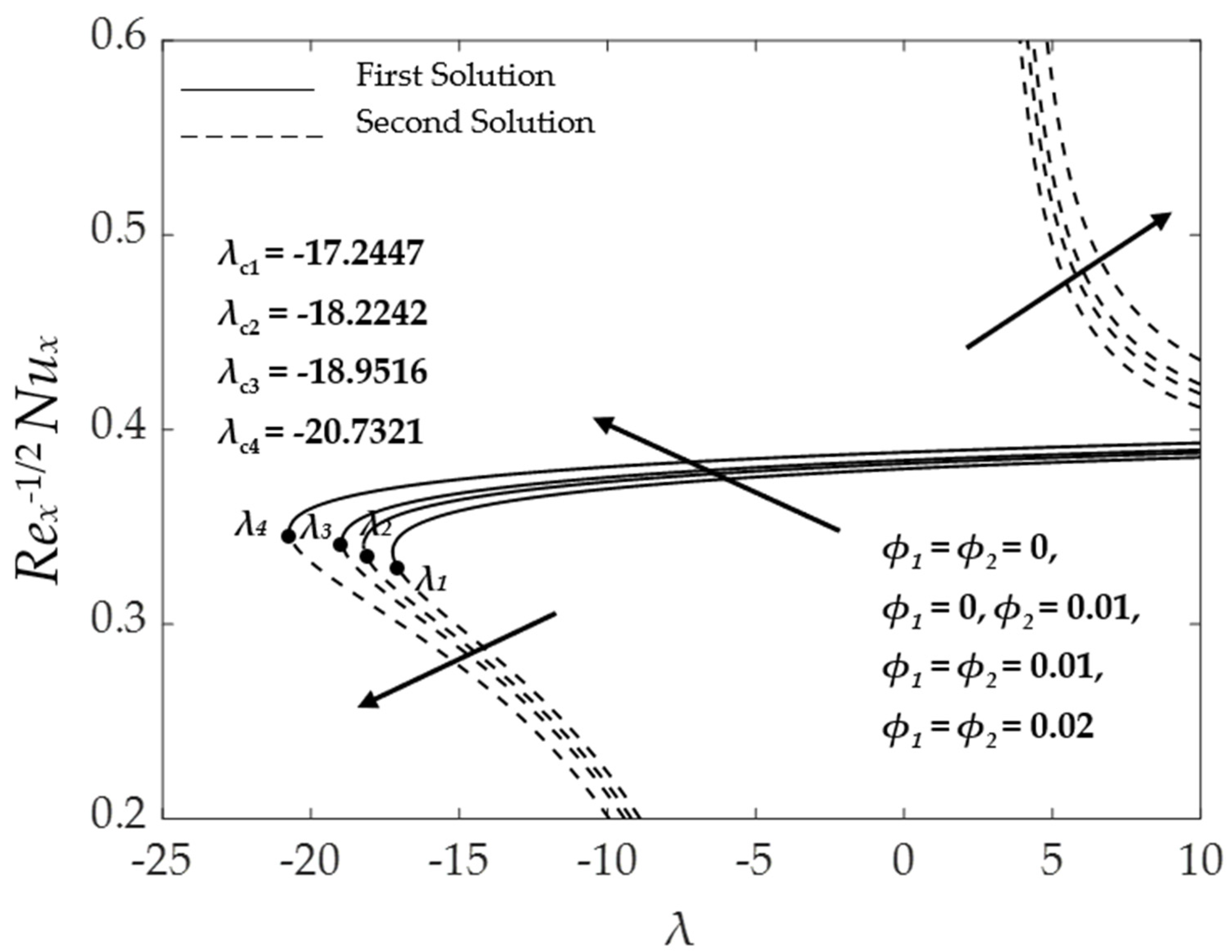
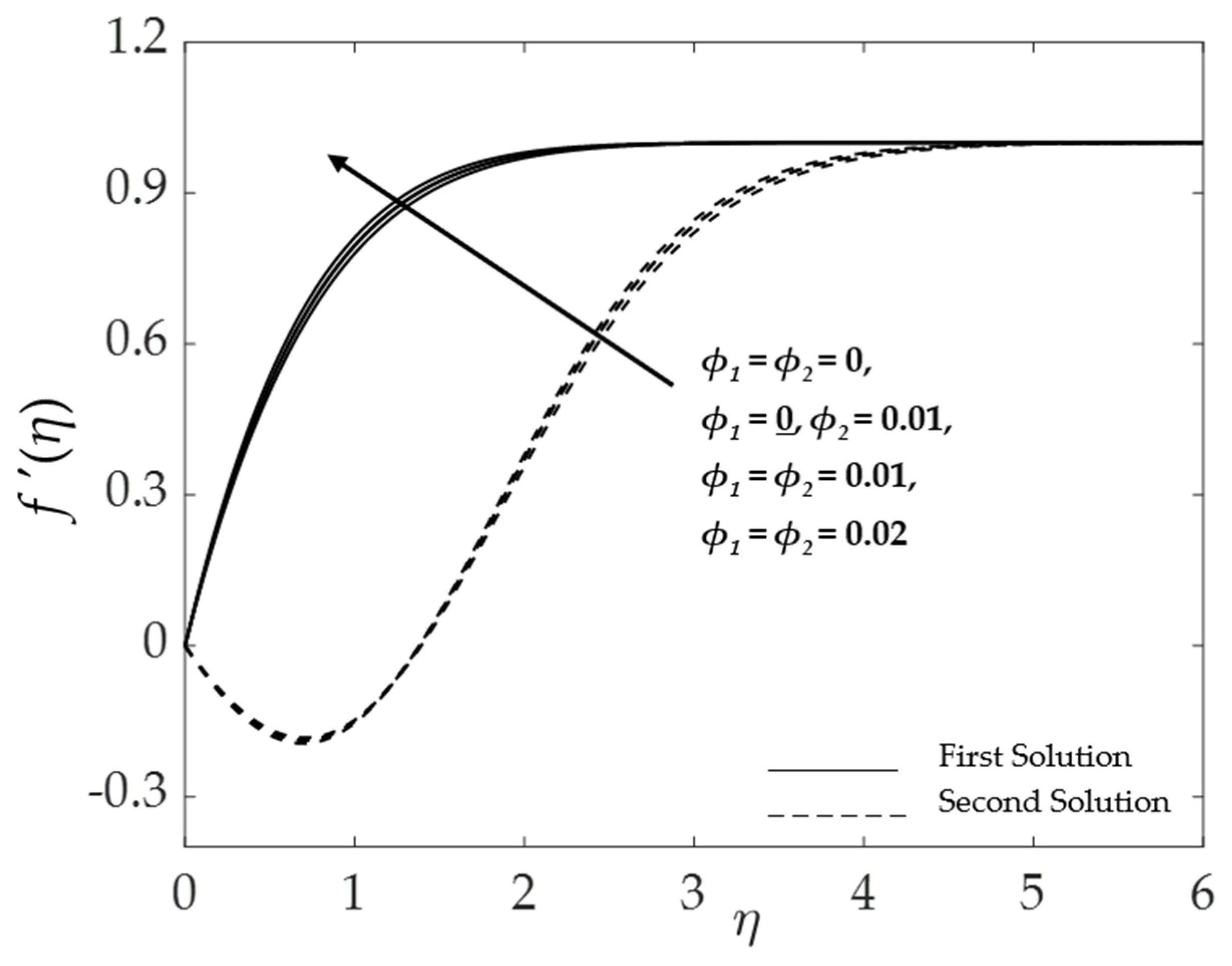
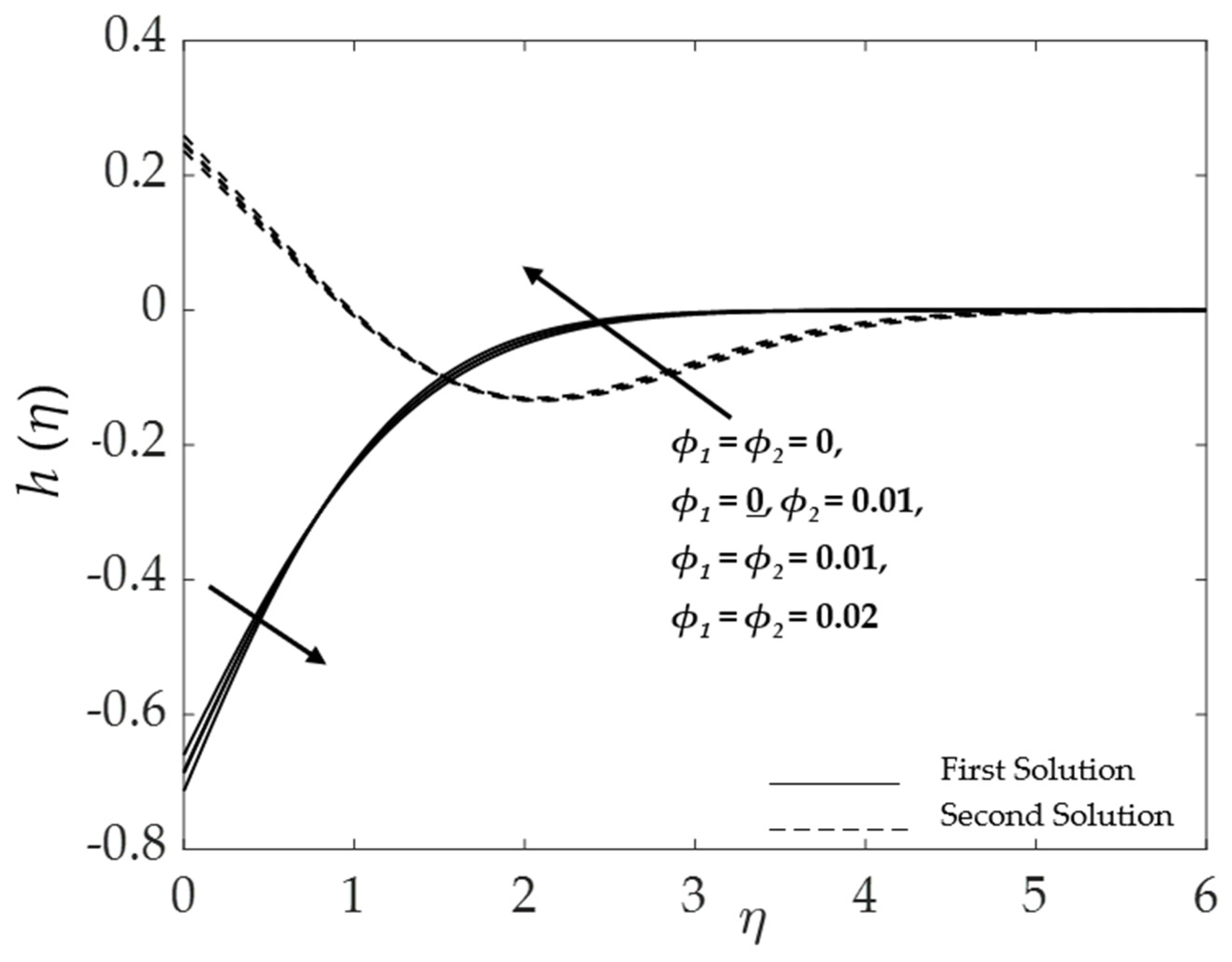
4.2. Effect of the Hybrid Nanoparticles Volume Fraction $\left({\varphi }_1,{\varphi }_2\right)$

Figure 7, Figure 8 and Figure 9 elucidate the influences of the hybrid nanoparticles volume fraction ${\varphi }_1,{\varphi }_2$ on the values of ${\mathit{Re}}_x{}^{1/2}{C}_f$, ${\mathit{Re}}_x{M}_x$, and ${\mathit{Re}}_x{}^{-1/2}N{u}_x$, respectively, for the various values of M = 1, Bi = n = 0.5, and $K=1$. It is discovered that critical value ${\lambda }_c$ for the pure water $\left({\varphi }_1={\varphi }_2=0\%\right)$ is −17.2447, for the $\mathrm{C}\mathrm{u}/{\mathrm{H}}_2\mathrm{O}$ nanofluid $\left({\varphi }_1=0\%, {\varphi }_2=1\%\right)$ is −18.2242, and for the $\mathrm{A}{\mathrm{l}}_2{\mathrm{O}}_3-\mathrm{C}\mathrm{u}/{\mathrm{H}}_2\mathrm{O}$ HNF $\left({\varphi }_1={\varphi }_2=1\% \mathrm{and} {\varphi }_1={\varphi }_2=2\%\right)$ are −18.9516 and −20.7321, respectively. Figure 7 and Figure 8 illustrate a similar profile pattern as the hybrid nanoparticles volume fraction increases will augment the values of ${\mathit{Re}}_x{}^{1/2}{C}_f$ and ${\mathit{Re}}_x{M}_x$ for the first solution but reduce for the second solution. It is noted that, between those base fluid, $\mathrm{C}\mathrm{u}/{\mathrm{H}}_2\mathrm{O}$ nanofluid, and $\mathrm{A}{\mathrm{l}}_2{\mathrm{O}}_3-\mathrm{C}\mathrm{u}/{\mathrm{H}}_2\mathrm{O}$ HNF, the highest critical value is $\mathrm{A}{\mathrm{l}}_2{\mathrm{O}}_3-\mathrm{C}\mathrm{u}/{\mathrm{H}}_2\mathrm{O}$ HNF $\left({\varphi }_1={\varphi }_2=2\%\right)$. This is because the augmentation of the nanoparticles’ volume fraction will improve the viscosity performance of the fluid as well as enhance the surface shear stress, leading to an increase in local skin friction ${\mathit{Re}}_x{}^{1/2}{C}_f$. Additionally, Figure 9 shows that the ${\mathit{Re}}_x{}^{-1/2}N{u}_x$ inclines to the larger value of nanoparticle volume fraction for the first solution as well. However, for the second solution, the ${\mathit{Re}}_x{}^{-1/2}N{u}_x$ value declines for the opposing region and rises for the assisting region as the ${\varphi }_1,{\varphi }_2$ increase. The addition of nanoparticles in the base fluid ($\mathrm{A}{\mathrm{l}}_2{\mathrm{O}}_3-\mathrm{C}\mathrm{u}/{\mathrm{H}}_2\mathrm{O}$ HNF) exerts more energy and raises the temperature, as well as increases the boundary layer thickness. This discovery proves that the HNF has greater heat transfer enhancement compared to nanofluid and water.

The effects of the hybrid nanoparticle volume fraction on the profiles are illustrated in Figure 10, Figure 11 and Figure 12 for the water $\left({\varphi }_1={\varphi }_2=0\%\right)$, the $\mathrm{C}\mathrm{u}/{\mathrm{H}}_2\mathrm{O}$ nanofluid $\left({\varphi }_1=0\%, {\varphi }_2=1\%\right)$, and the $\mathrm{A}{\mathrm{l}}_2{\mathrm{O}}_3-\mathrm{C}\mathrm{u}/{\mathrm{H}}_2\mathrm{O}$ HNF $\left({\varphi }_1={\varphi }_2=1\% \mathrm{and} {\varphi }_1={\varphi }_2=2\%\right)$. It is discovered that increasing the hybrid nanoparticles value causes the velocity profile as well as microrotation profile to rise for both solutions. However, the microrotation profile shows that the first solution depreciates at the beginning $\left(0\le \eta \le 1\right)$. The thickness of the momentum boundary layer decreases for both profiles due to the increased nanoparticle concentration. Hence, the fluid flow velocity escalates. Furthermore, as the hybrid nanoparticle volume fraction rises, the temperature profile for both outcomes decreases, and the thickness of the thermal boundary layer increases. Physically, HNF is a novel type of conventional fluid that has greater heat transfer enhancement (refer to Devi and Devi [35]; Suresh et al. [45]), perhaps due to the impacts on magnetic properties and the Biot number, which indicate that the consequence will be the reverse.

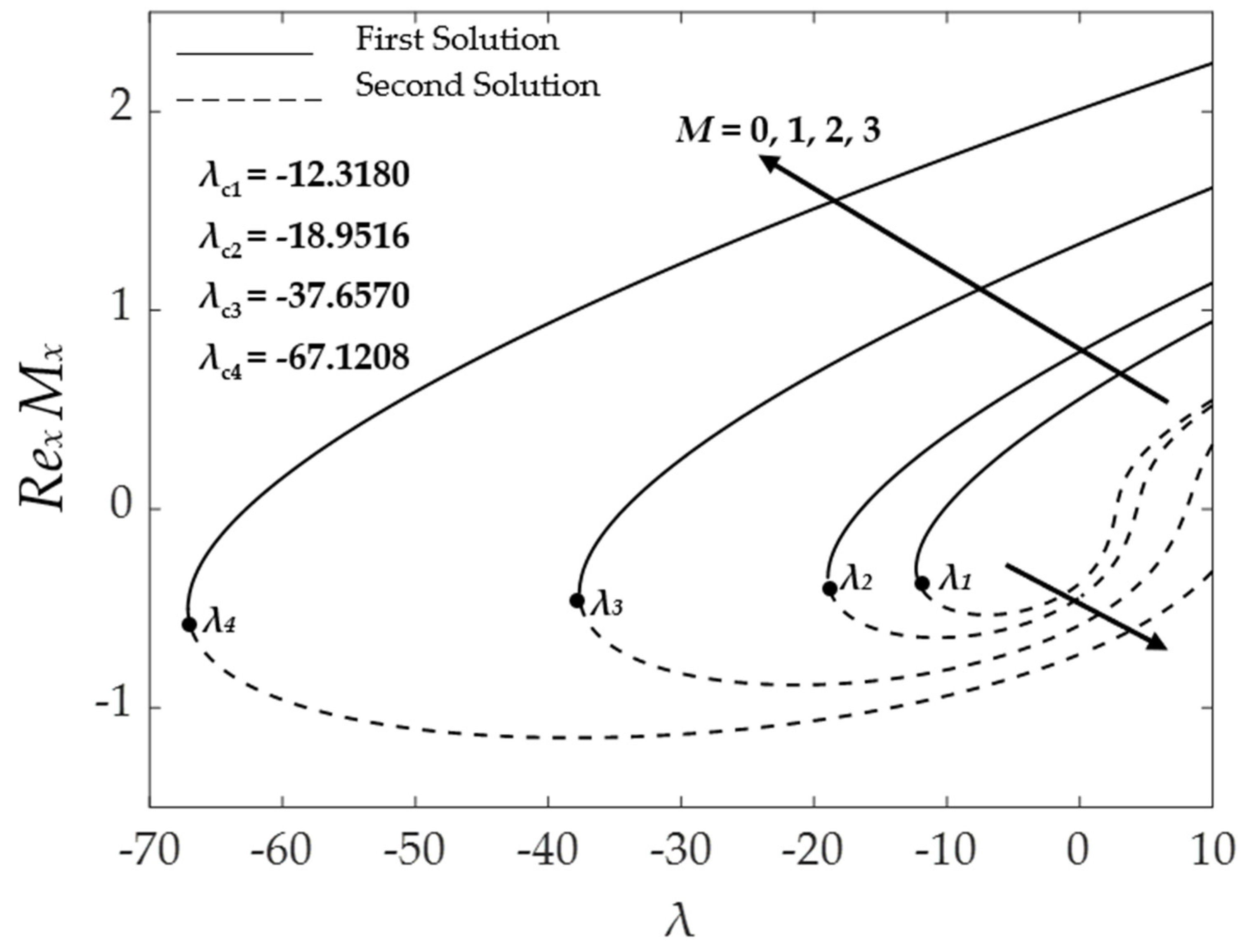
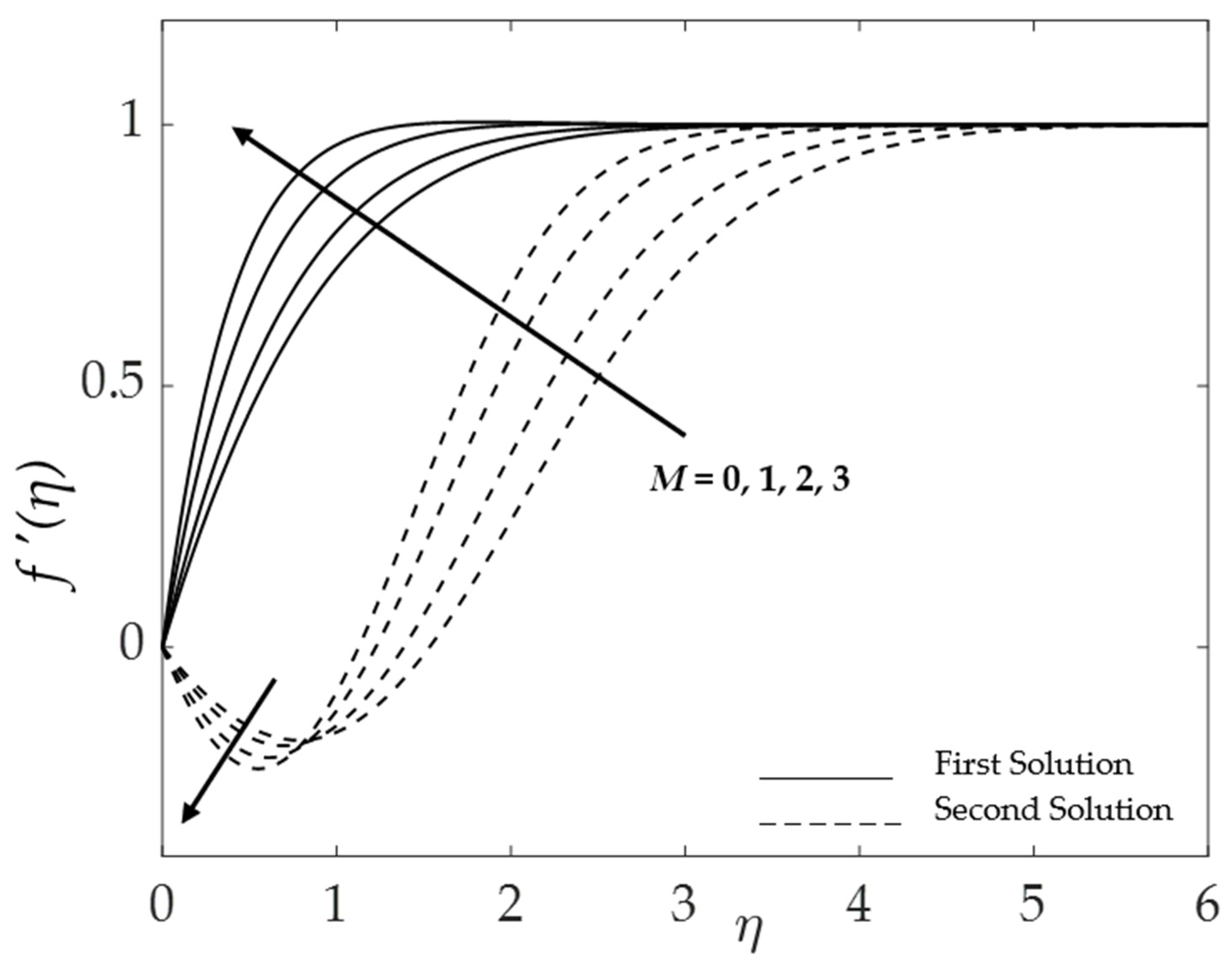
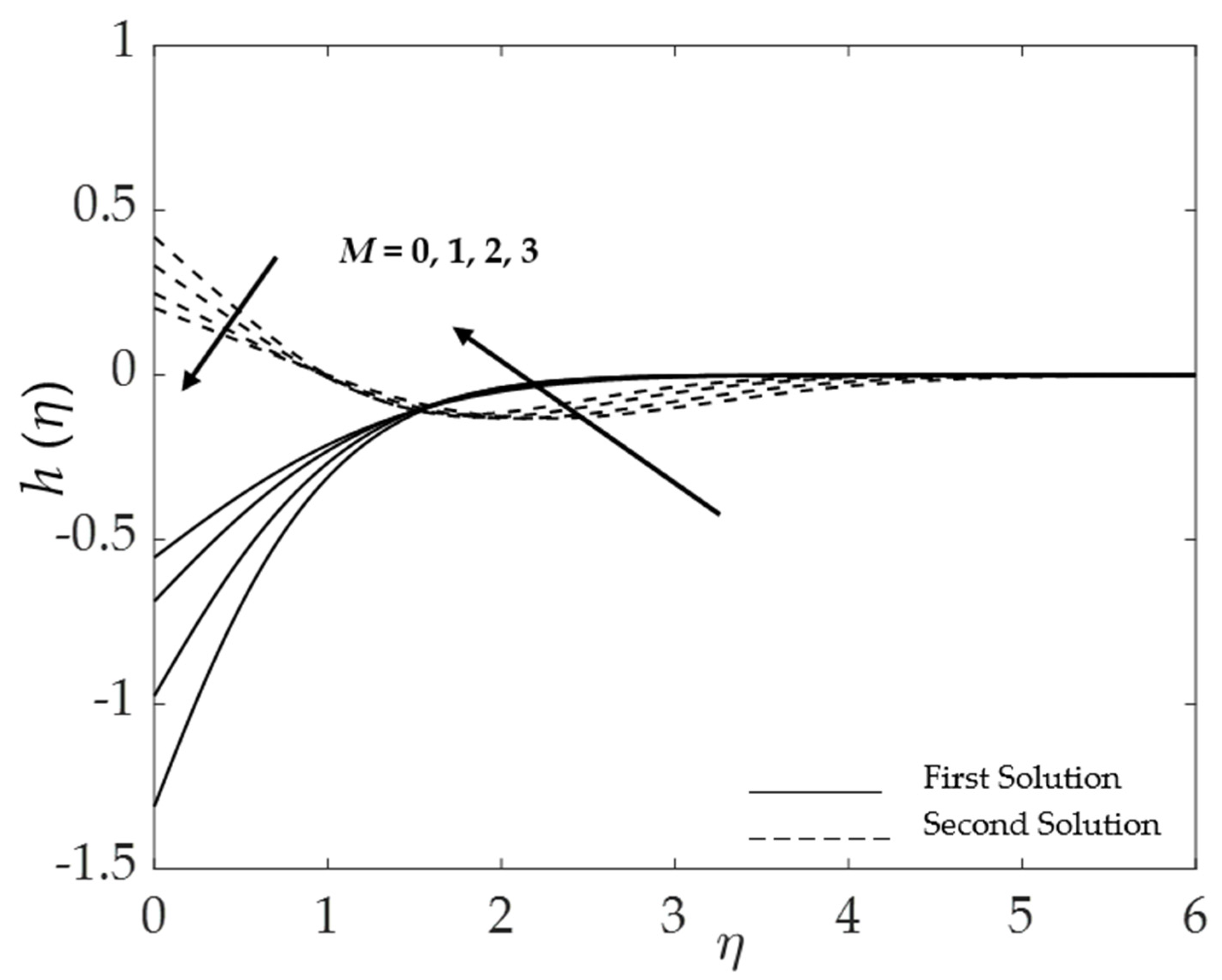
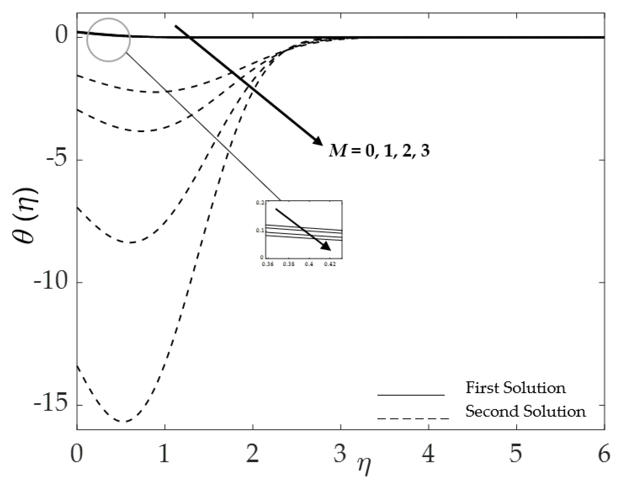
4.3. Effect of the Magnetic Parameter $\left(M\right)$

In addition, Figure 13, Figure 14 and Figure 15 display the changes in the values of ${\mathit{Re}}_x{}^{1/2}{C}_f$,${\mathrm{Re}}_x{M}_x$, and ${\mathit{Re}}_x{}^{-1/2}N{u}_x$, for some values of $M$. The critical values ${\lambda }_c$ for the magnetic parameters M = 0, 1, 2, and 3 are ${\lambda }_c$ = −12.3180, −18.9516, −37.6570, and −67.1208, respectively. It is observed that the presence of a magnetic field $\left(M>0\right)$ enhances the values of these physical quantities for the first solution but shows contrast for the second solution. The applied magnetic field exerts viscous drag forces on the flow field, which slows down the fluid’s motion and raises the skin friction coefficient as well as heat transfer on the surface. This is because the fluid’s flow is slowed down by the Lorentz force, which also creates a resistive force against it and, consequently, reduces the fluid velocity. Lorentz force also can be defined as the force exerted on a charged particle moving with velocity through an electric field and magnetic field.

Further, the effects on the profiles for some values of $M$ when $K=1$, Bi = n = 0.5, ${\varphi }_1={\varphi }_2=1\%$, and $\lambda =1$ are depicted in Figure 16, Figure 17 and Figure 18. It is found that the velocity profiles augment the larger values of magnetic parameters. As the magnetic parameter rises, the momentum boundary layer thins, resulting in delayed flow, which raises the fluid flow velocity. By referring to the delayed flow here, the magnetic parameter plays a role as a fluid flow controller that could prevent the occurrence of turbulence flow. This outcome is in line with that displayed in Figure 13. Meanwhile, the microrotation profiles elevate for both branches when the magnetic parameter increases. However, for the second solution, microrotation and velocity profiles reduce for the range of $\left(0\le \eta \le 1\right)$ and then monotonically increase for the range of $\left(\eta \ge 1\right)$. The high intensity of the magnetic field could also boost the rotation of the particles on the surface and, hence, increase the microrotation profile. Further, Figure 18 shows that as the magnetic parameter increases, the temperature profile decreases. The increase in the heat flux was caused by a reduction in the thermal boundary thickness. This result is consistent with Figure 15’s illustration.

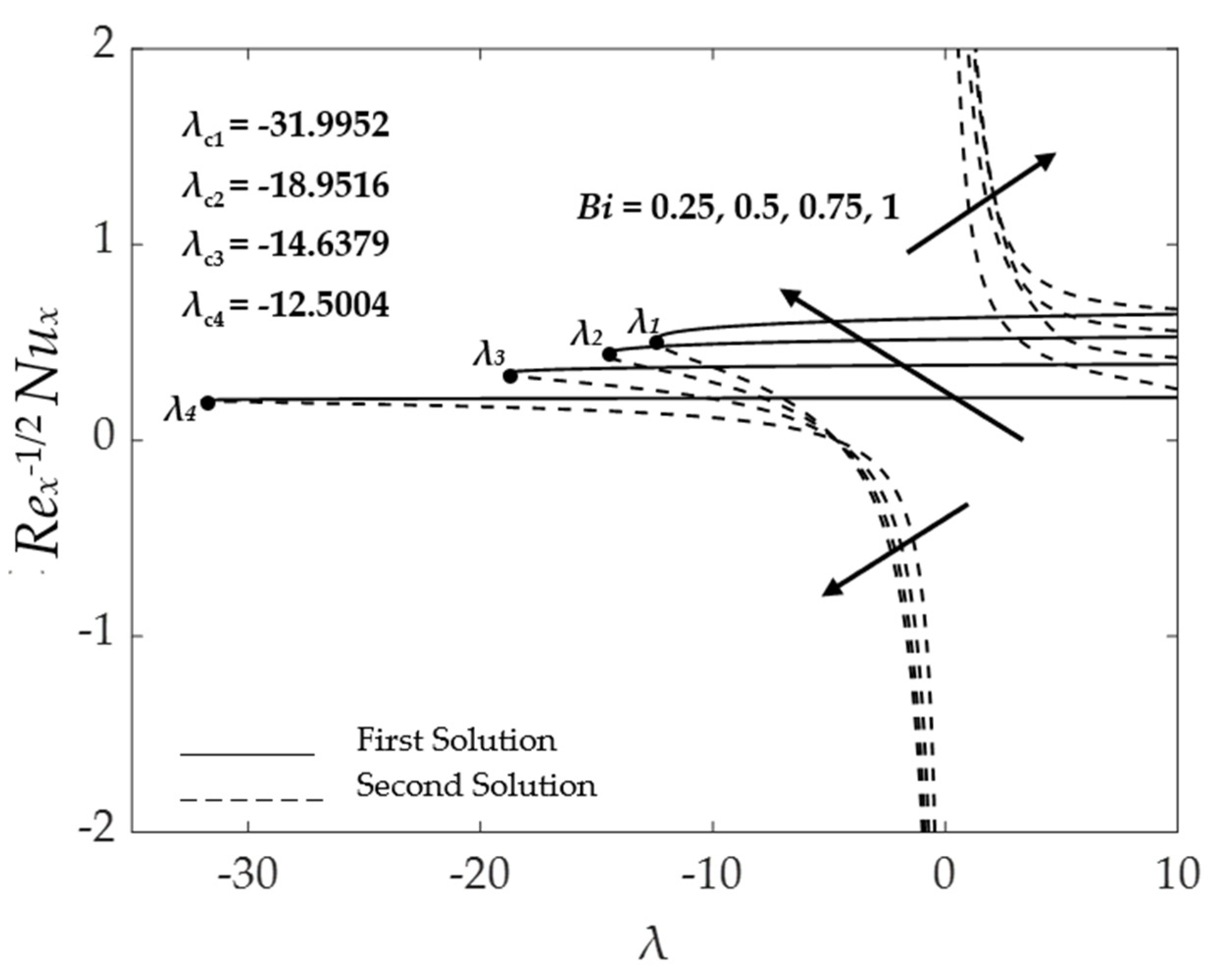
4.4. Effect of the Biot Number $\left(Bi\right)$

Effects of $Bi$ on the local Nusselt number ${\mathit{Re}}_x{}^{-1/2}N{u}_x$ with λ when $M=1$, $\mathrm{Pr}=6.2$, $n=0.5$ and ${\varphi }_1={\varphi }_2=1\%$ is shown in Figure 19. Physically, Biot number Bi is expressed as the measure of the interaction between convection at the surface of the body and conduction in the solid. There is an increase in the HTR for an increasing value of the Bi. As the Bi rises, the surface’s heat resistance decreases noticeably. Increased convection is the cause of the increased surface temperature. Additionally, the ratio that controls a body’s internal temperature changes significantly as the body warms or cools over time when a thermal gradient is applied to the surface. The critical values ${\lambda }_c$ for the $Bi$= 0.25, 0.5, 0.75, 1 are ${\lambda }_c$ = −31.9952, −18.9516, −14.6379, and −12.5004, respectively.

4.5. Stability Analysis

A stability analysis is performed to determine which one of the solutions is stable and which one is not. The eigenvalues $\gamma$ are found in (19), and these smallest eigenvalues $\gamma$ are illustrated in Figure 20 over the stretching or shrinking parameter $\lambda$ when $K=1$, Bi = n = 0.5, ${\varphi }_1={\varphi }_2=1\%$ and $M=1$. It is clearly showing the first solution has positive $\gamma$ while the second solution has negative $\gamma$, respectively. It is also noticed that, as $\lambda \to {\lambda }_c, \gamma \to 0$, this means that at turning points (from the first to the second solution), there is a change in the values of $\lambda$ from stable (positive) to unstable (negative). Thus, this validates the stability analysis in the current work, and hence, it is probable that the first solution is more stable than the second solution.

5. Conclusions

This study explores the MHD MF flow consisting of HNF along with a vertical surface with a convective BC. By using the dimensionless set of variables, the resulting equations of ODEs are solved numerically using the bvp4c solver in MATLAB. Both a numerical and graphical analysis of the dimensionless parameters is performed. Apart from that, the present study also considers the magnetic field in a micropolar hybrid nanofluid. MHD could help to control the behavior of the fluid flow, for example, to prevent the occurrence of turbulence flow. Thus, the following is a list of the findings in summary:

For both $\lambda =\pm 1$ regions, a dual solution is present, and the critical values ${\lambda }_c$ are discovered for the $\lambda <0$ region.

An increase in K will raise the Re_x^1/2 C_f, and Re_x M_x, whereas it will decline the Re_x^−1/2 Nu_x, respectively.

Between those types of water (ϕ₁ = ϕ₂ = 0%), the nanofluid (ϕ₁ = 0%, ϕ₂ = 1%) and the HNF (ϕ₁ = ϕ₂ = 1% and ϕ₁ = ϕ₂ = 2%), it is observed that the highest critical value is the HNF (ϕ₁ = ϕ₂ = 2%). The upsurges of the nanoparticle volume fraction boost the dynamic viscosity performance and surface shear stress.

The physical quantities Re_x^1/2 C_f, Re_x M_x, and Re_x^−1/2 Nu_x rise for the increasing values of the nanoparticle volume fraction and magnetic field parameter.

For higher values of the Bi, there is an increase in the HTR.

The stability inquiry proves that the first solution is physically reliable and stable.

References

1. Soid, S.K.; Ishak, A.; Pop, I. MHD stagnation-point flow over a stretching/shrinking sheet in a micropolar fluid with a slip boundary. Sains Malays. 2018, 47, 2907–2916. [Google Scholar] [CrossRef]
2. Eringen, A. Theory of Micropolar Fluids. Indiana Univ. Math. J. 1966, 16, 1–18. [Google Scholar] [CrossRef]
3. Ishak, A. Thermal boundary layer flow over a stretching sheet in a micropolar fluid with radiation effect. Meccanica 2010, 45, 367–373. [Google Scholar] [CrossRef]
4. Uddin, M.S.; Bhattacharyya, K.; Shafie, S. Micropolar fluid flow and heat transfer over an exponentially permeable shrinking sheet. Propuls. Power Res. 2016, 5, 310–317. [Google Scholar] [CrossRef]
5. Nazar, R.; Amin, N.; Pop, I. Unsteady boundary layer flow due to a stretching surface in a rotating fluid. Mech. Res. Commun. 2004, 31, 121–128. [Google Scholar] [CrossRef]
6. Nadeem, S.; Hussain, M.; Naz, M. MHD stagnation flow of a micropolar fluid through a porous medium. Meccanica 2010, 45, 869–880. [Google Scholar] [CrossRef]
7. Ishak, A.; Lok, Y.Y.; Pop, I. Stagnation-point flow over a shrinking sheet in a micropolar fluid. Chem. Eng. Commun. 2010, 197, 1417–1427. [Google Scholar] [CrossRef]
8. Noor, N.F.M.; Haq, R.U.; Nadeem, S.; Hashim, I. Mixed convection stagnation flow of a micropolar nanofluid along a vertically stretching surface with slip effects. Meccanica 2015, 50, 2007–2022. [Google Scholar] [CrossRef]
9. Ul Haq, R.; Nadeem, S.; Akbar, N.S.; Khan, Z.H. Buoyancy and radiation effect on stagnation point flow of micropolar nanofluid along a vertically convective stretching surface. IEEE Trans. Nanotechnol. 2015, 14, 42–50. [Google Scholar] [CrossRef]
10. Ramachandran, P.S.; Mathur, M.N. Heat transfer in the stagnation point flow of a micropolar fluid. Acta Mech. 1980, 36, 247–261. [Google Scholar] [CrossRef]
11. Guram, G.S.; Smith, A.C. Stagnation flows of micropolar fluids with strong and weak interactions. Comput. Math. Appl. 1980, 6, 213–233. [Google Scholar] [CrossRef] [Green Version]
12. Nazar, R.; Amin, N.; Filip, D.; Pop, I. Stagnation point flow of a micropolar fluid towards a stretching sheet. Int. J. Non-Linear Mech. 2004, 39, 1227–1235. [Google Scholar] [CrossRef]
13. Khashi’ie, N.S.; Arifin, N.M.; Nazar, R.; Hafidzuddin, E.H.; Wahi, N.; Pop, I. Mixed convective flow and heat transfer of a dual stratified micropolar fluid induced by a permeable stretching/shrinking sheet. Entropy 2019, 21, 1162. [Google Scholar] [CrossRef] [Green Version]
14. Subhani, M.; Nadeem, S. Numerical analysis of micropolar hybrid nanofluid. Appl. Nanosci. 2019, 9, 447–459. [Google Scholar] [CrossRef]
15. Olayemi, O.A.; Al-Farhany, K.; Obalalu, A.M.; Ajide, T.F.; Adebayo, K.R. Magnetoconvection around an elliptic cylinder placed in a lid-driven square enclosure subjected to internal heat generation or absorption. Heat Transf. 2022, 51, 4950–4976. [Google Scholar] [CrossRef]
16. Mishra, N.K.; Sharma, M.; Sharma, B.K.; Khanduri, U. Soret and Dufour effects on MHD nanofluid flow of blood through a stenosed artery with variable viscosity. Int. J. Mod. Phys. B 2023, 2350266. [Google Scholar] [CrossRef]
17. Nabwey, H.A.; Mahdy, A. Transient flow of micropolar dusty hybrid nanofluid loaded with Fe3O4-Ag nanoparticles through a porous stretching sheet. Results Phys. 2021, 21, 103777. [Google Scholar] [CrossRef]
18. Lund, L.A.; Omar, Z.; Khan, I.; Sherif, E.-S.M. Dual Solutions and Stability Analysis of a Hybrid Nanofluid over a Stretching/Shrinking Sheet Executing MHD Flow. Symmetry 2020, 12, 276. [Google Scholar] [CrossRef] [Green Version]
19. Goldanlou, A.S.; Badri, M.; Heidarshenas, B.; Hussein, A.K.; Rostami, S.; Shadloo, M.S. Numerical investigation on forced hybrid nanofluid flow and heat transfer inside a three-dimensional annulus equipped with hot and cold rods: Using symmetry simulation. Symmetry 2020, 12, 1873. [Google Scholar] [CrossRef]
20. Zainal, N.A.; Nazar, R.; Naganthran, K.; Pop, I. MHD mixed convection stagnation point flow of a hybrid nanofluid past a vertical flat plate with convective boundary condition. Chin. J. Phys. 2020, 66, 630–644. [Google Scholar] [CrossRef]
21. Obalalu, A.M.; Ahmad, H.; Salawu, S.O.; Olayemi, O.A.; Odetunde, C.B.; Ajala, A.O.; Abdulraheem, A. Improvement of mechanical energy using thermal efficiency of hybrid nanofluid on solar aircraft wings: An application of renewable, sustainable energy. In Waves in Random and Complex Media; Taylor & Francis Group: London, UK, 2023; pp. 1–30. [Google Scholar] [CrossRef]
22. Nadeem, S.; Abbas, N. On both MHD and slip effect in micropolar hybrid nanofluid past a circular cylinder under stagnation point region. Can. J. Phys. 2019, 97, 392–399. [Google Scholar] [CrossRef]
23. Khan, U.; Zaib, A.; Pop, I.; Abu Bakar, S.; Ishak, A. Stagnation point flow of a micropolar fluid filled with hybrid nanoparticles by considering various base fluids and nanoparticle shape factors. Int. J. Numer. Methods Heat Fluid Flow 2021, 32, 2320–2344. [Google Scholar] [CrossRef]
24. Waini, I.; Ishak, A.; Pop, I. Radiative and magnetohydrodynamic micropolar hybrid nanofluid flow over a shrinking sheet with Joule heating and viscous dissipation effects. Neural Comput. Appl. 2022, 34, 3783–3794. [Google Scholar] [CrossRef]
25. Anuar, N.S.; Bachok, N. Double solutions and stability analysis of micropolar hybrid nanofluid with thermal radiation impact on unsteady stagnation point flow. Mathematics 2021, 9, 276. [Google Scholar] [CrossRef]
26. Haider, M.I.; Asjad, M.I.; Ali, R.; Ghaemi, F.; Ahmadian, A. Heat transfer analysis of micropolar hybrid nanofluid over an oscillating vertical plate and Newtonian heating. J. Therm. Anal. Calorim. 2021, 144, 2079–2090. [Google Scholar] [CrossRef]
27. Al-Hanaya, A.M.; Sajid, F.; Abbas, N.; Nadeem, S. Effect of SWCNT and MWCNT on the flow of micropolar hybrid nanofluid over a curved stretching surface with induced magnetic field. Sci. Rep. 2020, 10, 8488. [Google Scholar] [CrossRef]
28. Sharma, B.K.; Khanduri, U.; Mishra, N.K.; Chamkha, A.J. Analysis of Arrhenius activation energy on magnetohydrodynamic gyrotactic microorganism flow through porous medium over an inclined stretching sheet with thermophoresis and Brownian motion. Proc. Inst. Mech. Eng. Part E J. Process Mech. Eng. 2022, 09544089221128768. [Google Scholar] [CrossRef]
29. Sharma, B.K.; Gandhi, R. Combined effects of Joule heating and non-uniform heat source/sink on unsteady MHD mixed convective flow over a vertical stretching surface embedded in a Darcy-Forchheimer porous medium. Propuls. Power Res. 2022, 11, 276–292. [Google Scholar] [CrossRef]
30. Gandhi, R.; Sharma, B.K.; Mishra, N.K.; Al-Mdallal, Q.M. Computer Simulations of EMHD Casson Nanofluid Flow of Blood through an Irregular Stenotic Permeable Artery: Application of Koo-Kleinstreuer-Li Correlations. Nanomaterials 2023, 13, 652. [Google Scholar] [CrossRef]
31. Obalalu, A.M.; Wahaab, F.A.; Adebayo, L.L. Heat transfer in an unsteady vertical porous channel with injection/suction in the presence of heat generation. J. Taibah Univ. Sci. 2020, 14, 541–548. [Google Scholar] [CrossRef] [Green Version]
32. Obalalu, A.M. Heat and mass transfer in an unsteady squeezed Casson fluid flow with novel thermophysical properties: Analytical and numerical solution. Heat Transf. 2021, 50, 7988–8011. [Google Scholar] [CrossRef]
33. Devi, S.S.U.; Devi, S.P.A. Heat transfer enhancement of Cu−Al2O3/water hybrid nanofluid flow over a stretching sheet. J. Niger. Math. Soc. 2017, 36, 419–433. [Google Scholar]
34. Takabi, B.; Salehi, S. Augmentation of the heat transfer performance of a sinusoidal corrugated enclosure by employing hybrid nanofluid. Adv. Mech. Eng. 2014, 2014, 147059. [Google Scholar] [CrossRef]
35. Devi, S.S.U.; Devi, S.P.A. Numerical investigation of three-dimensional hybrid Cu-Al2O3/water nanofluid flow over a stretching sheet with effecting Lorentz force subject to Newtonian heating. Can. J. Phys. 2016, 94, 490–496. [Google Scholar] [CrossRef]
36. Roşca, A.V.; Roşca, N.C.; Pop, I. Mixed convection stagnation point flow of a hybrid nanofluid past a vertical flat plate with a second order velocity model. Int. J. Numer. Methods Heat Fluid Flow 2020, 31, 75–91. [Google Scholar] [CrossRef]
37. Waini, I.; Ishak, A.; Pop, I. Mixed convection flow over an exponentially stretching/shrinking vertical surface in a hybrid nanofluid. Alex. Eng. J. 2020, 59, 1881–1891. [Google Scholar] [CrossRef]
38. Oztop, H.F.; Abu-Nada, E. Numerical study of natural convection in partially heated rectangular enclosures filled with nanofluids. Int. J. Heat Fluid Flow 2008, 29, 1326–1336. [Google Scholar] [CrossRef]
39. Weidman, P. Axisymmetric rotational stagnation point flow impinging on a radially stretching sheet. Int. J. Non-Linear Mech. 2016, 82, 1–5. [Google Scholar] [CrossRef]
40. Merkin, J.H. On dual solutions occurring in mixed convection in a porous medium. J. Eng. Math. 1986, 20, 171–179. [Google Scholar] [CrossRef]
41. Weidman, P.D.; Kubitschek, D.G.; Davis, A.M.J. The effect of transpiration on self-similar boundary layer flow over moving surfaces. Int. J. Eng. Sci. 2006, 44, 730–737. [Google Scholar] [CrossRef]
42. Harris, S.D.; Ingham, D.B.; Pop, I. Mixed convection boundary-layer flow near the stagnation point on a vertical surface in a porous medium: Brinkman model with slip. Transp. Porous Media 2009, 77, 267–285. [Google Scholar] [CrossRef]
43. Shampine, L.F.; Gladwell, I.; Thompson, S. Solving ODEs with MATHLAB; Cambridge University Press: Cambridge, UK, 2003; ISBN 9780521824040. [Google Scholar]
44. Khashi’ie, N.S.; Arifin, N.M.; Pop, I. Mixed convective stagnation point flow towards a vertical riga plate in hybrid Cu-Al2O3/water nanofluid. Mathematics 2020, 8, 912. [Google Scholar] [CrossRef]
45. Suresh, S.; Venkitaraj, K.P.; Selvakumar, P.; Chandrasekar, M. Synthesis of Al2O3-Cu/water hybrid nanofluids using two step method and its thermo physical properties. Colloids Surfaces A Physicochem. Eng. Asp. 2011, 388, 41–48. [Google Scholar] [CrossRef]
Figure 1. Physical model.
Symmetry 15 00920 g001
Figure 2. Difference of Rex1/2 Cf for some values of K when M = 1, Bi = n = 0.5, and ϕ1 = ϕ2 = 0.01.
Symmetry 15 00920 g002
Figure 3. Difference of Rex−1/2 Nux for some values of K when M = 1, Bi = n = 0.5, and ϕ1 = ϕ2 = 0.01.
Symmetry 15 00920 g003
Figure 4. Influence of K on f ’(η) when M = 1, Bi = n= 0.5, ϕ1 = ϕ2 = 0.01, and λ = 1.
Symmetry 15 00920 g004
Figure 5. Influence of K on h(η) when M = 1, Bi = n = 0.5, ϕ1 = ϕ2 = 0.01, and λ = 1.
Symmetry 15 00920 g005
Figure 6. Influence of K on θ(0) when M = 1, Bi = n = 0.5, ϕ1 = ϕ2 = 0.01, and λ = 1.
Symmetry 15 00920 g006
Figure 7. Difference of Rex1/2 Cf for some values of ϕ1, ϕ2 when M = 1, Bi = n = 0.5, and K = 1.
Symmetry 15 00920 g007
Figure 8. Difference of Rex Mx for some values of ϕ1, ϕ2 when M = 1, Bi = n = 0.5, and K = 1.
Symmetry 15 00920 g008
Figure 9. Difference of Rex−1/2 Nux for some values of ϕ1, ϕ2 when M = 1, Bi = n = 0.5, and K = 1.
Symmetry 15 00920 g009
Figure 10. Influence of ϕ1, ϕ2 on f ’(η) when M = 1, Bi = n = 0.5, K = 1, and λ = 1.
Symmetry 15 00920 g010
Figure 11. Influence of ϕ1, ϕ2 on h(η) when M = 1, Bi = n = 0.5, K = 1, and λ = 1.
Symmetry 15 00920 g011
Figure 12. Influence of ϕ1, ϕ2 on θ(0) when M = 1, Bi = n = 0.5, K = 1, and λ = 1.
Symmetry 15 00920 g012
Figure 13. Difference of Rex1/2 Cf for some values of M when K = 1, Bi = n = 0.5, and ϕ1 = ϕ2 = 0.01.
Symmetry 15 00920 g013
Figure 14. Difference of Rex Mx for some values of M when K = 1, Bi = n = 0.5, and ϕ1 = ϕ2 = 0.01.
Symmetry 15 00920 g014
Figure 15. Difference of Rex−1/2 Nux for some values of M when K = 1, Bi = n = 0.5, and ϕ1 = ϕ2 = 0.01.
Symmetry 15 00920 g015
Figure 16. Influence of M on f ’(η) when K = 1, Bi = n= 0.5, ϕ1 = ϕ2 = 0.01, and λ = 1.
Symmetry 15 00920 g016
Figure 17. Influence of M on h(η) when K = 1, Bi = n = 0.5, ϕ1 = ϕ2 = 0.01, and λ = 1.
Symmetry 15 00920 g017
Figure 18. Influence of M on θ(0) when K = 1, Bi = n = 0.5, ϕ1 = ϕ2 = 0.01, and λ = 1.
Symmetry 15 00920 g018
Figure 19. Difference of Rex−1/2 Nux for some values of Bi when K = 1, M = 1, n= 0.5, and ϕ1 = ϕ2 = 0.01.
Symmetry 15 00920 g019
Figure 20. Eigenvalues γ toward λ when K = M = 1, Bi = n = 0.5, and ϕ1 = ϕ2 = 0.01.
Symmetry 15 00920 g020