Abstract
The inverse conductivity problem in electrical impedance tomography involves the solving of a nonlinear and under-determined system of equations. This paper presents a new approach, which leads to a quadratic and overdetermined system of equations. The aim of the paper is to establish new research directions in handling of the inverse conductivity problem. The basis of the proposed method is that the material, which can be considered as an isotropic continuum, is modeled as a linear network with concentrated parameters. The weights of the obtained graph represent the properties of the discretized continuum. Further, the application of the developed procedure allows for the dielectric constant to be used in the multi-frequency approach, as a result of which the optimized system of equations always remains overdetermined. Through case studies, the efficacy of the reconstruction method by changing the mesh resolution applied for discretizing is presented and evaluated. The presented results show, that, due to the application of discrete, symmetric mathematical structures, the new approach even at coarse mesh resolution is capable of localizing the inhomogeneities of the material.
1. Introduction
In electrical impedance tomography (EIT), the main goal is to determine the conductivity distribution of the investigated material. In order to complete this task, an electric field inside the examined object is created, and by measuring certain parameters (e.g., potentials or voltages) on its surface, the distribution of the complex electrical conductivity of the given object can be deduced. The success of the EIT application is based solely on the quality of reconstructed images; however, research on algorithms for solving the EIT inverse problem took place until the mid-1990s without any real progress in this field. Researchers at that time mainly tried to adapt existing algorithms to the scope of the EIT’s problems [1].
Considering that during the application of EIT, the excitation is done with direct or sinusoidal alternating current, and that the measurement is basically carried out at a low frequency (maximum frequency is usually 100 kHz), and assuming that the magnetic phenomena arising during the measurement are negligible, the basic partial differential equation (PDE) of EIT can be expressed as [1]:
where
;
denotes the conductivity;
denotes the permittivity;
denotes the electric potential;
denotes the vector of spatial coordinates.
In Equation (1), , , and also are dependent (two- or three-variable) functions. Equation (1) for u can usually be solved numerically by specifying Dirichlet, Neumann, or Robin boundary conditions [2]. In order to be able to implement the mathematical image reconstruction of the EIT (another algorithm can be chosen as well), it is necessary to define two main problems: the direct problem and the inverse problem [1]. The direct problem is actually the numerical solution of Equation (1) for u with appropriate boundary conditions. The direct problem is well-conditioned, thus the solution of this and similar mathematical problems has been known for decades and can be routinely used in technical practice. The most famous numerical methods that can be applied as a direct solver are (non-exhaustive):
- -
- Finite Difference Method (FD) [2];
- -
- Finite Element Method (FEM) [3,4];
- -
- Boundary Element Method (BEM) [2].
Among the listed methods, FEM can be considered the most widespread and the most accepted. In this manner, software solutions have been developed that can be applied at the user level, requiring minimal knowledge of numerical methods [1].
One of the first publications that defines the inverse conductivity problem (the reconstruction of the function in Equation (1)) is attributed to Calderón et al. [5]. Calderón’s article published in 1980 is epoch-making in the formulation of EIT. According to Calderón, the inverse problem generally means determining the conductivity of a region given by the boundary conditions. General formulation is important due to the mathematical formalization, as well as the diverse application potential (geophysics, medicine, chemical industry, etc.). Calderón proved that in the case of a linearized problem and a constant conductivity function, the values measured at the boundary during measurements depend non-linearly on the conductivity distribution of the material, and the clarity of this non-linear relationship was also proved by Calderón [5].
On the other hand, the inverse problem represents a bigger and almost impossible ill-conditioned challenge for researchers. In many cases, the difficulties occur in the area of uniqueness of the various numerical reconstruction procedures because, in that case, a wide variety of conductivity distributions can result in the same measured values [1]. This can lead to the fact that, in many cases, the reconstructed conductivity distribution does not even come close to the real one (seems unrealistic). Since the measured data are loaded with noise, the error phenomenon increases in this case. It is possible to restrict the reconstruction to a controllable framework (e.g., regularization, or by applying different conditions, such as the conductivity distribution being smooth, accepting only positive values, etc.); however, in many cases, this is not sufficient, thus the restored image is not close to the real one [1]. As the ill-conditioned behavior increases with increasing resolution, the sensitivity decreases by moving towards the center of the examined object (this can lead to the point where objects will not be noticed). Therefore, with the help of the developed methods, and compared to other imaging procedures, the creation of high-resolution images already seems to be almost impossible [1]. This problem can be even more difficult during the transition from 2D to 3D, since in the case of the EIT (since the electric field is 3D), a 3D image cannot be assembled from 2D sections. 3D imaging represents another physical problem [1]. Based on these observations, the conclusion is that the emergence of reliable, robust and accessible EIT devices still appears to be very far away, since in addition to the technical problems of measurement, the obstacles posed by image reconstruction are also waiting to be solved.
All these problems are proven by the extremely large amount of literature that deals exclusively with the solution of the Calderón problem. The literature related to EIT is extensive, and it is therefore difficult for researchers to examine all of it [1]. Despite the fact that the peak of EIT research can be roughly dated to between 1985 and 2005, the number of industrial applications based on it is minimal despite two decades’ worth of research work that covers almost the entire world [1]. Based on these facts, it can be truly concluded that the procedure itself cannot be considered mature at all [1]. This does not mean that research is not currently being conducted on this topic; nevertheless, the intensity of the research is significantly decreasing, as can be clearly seen from the publication dates of the included references.
The proposed methods developed during research thus far suggest a completely new approach to the inverse conductivity problem that could be solved during the implementation of the EIT procedure [6]. These methods put the 2D and 3D modeling of the direct and inverse problem on a new basis, creating a new, self-developed procedure, which is thus completely competitive with the state-of-the-art methods and, in many cases, even surpasses them. The motivation of the present research is to formulate the inverse conductivity problem using a new approach, in addition to using the numerical methods that have already been developed and tested. The aim is to use new numerical tools to open up new research directions to increase the efficiency and the robustness of the technology. After all, the new numerical method uses a new discretization procedure, which transforms the geometric properties of the investigated domain, as well as the isotropic conductivity and dielectric constant functions interpreted within the physical domain, into a system of linear equations with special properties. Among its beneficial properties, symmetry in discrete operators resulting from the isotropy of , the strict fulfillment of the global and local preservation principles, is used mostly during the reconstruction. Moreover, the matrix of the system of equations is a weighted Laplacian, and its advantageous properties are also known from the literature [6].
Considering this, this paper will present a novel numerical method to solve Equation (1) with special boundary conditions and to solve the inverse conductivity problem by taking advantage of the properties of the system of linear equations obtained during discretization (e.g., local conservation law, etc.). Naturally, to introduce the proposed method, first the structuring of multi-frequency data is presented for the simulation in order to achieve overdetermination, and other numerical methods necessary for the implementation of reconstruction will be discussed. Certainly, to prove the efficiency of the method, case studies for three different triangle mesh resolutions will be introduced in a separate section.
This paper is structured as follows. Section 1 is the introduction, Section 2 summarizes the related works, and Section 3 presents the specific numerical solution procedure developed for the direct problem, the data collection strategy, and the general numerical methods for solving inverse problems. Section 4 contains the detailed description of the algorithms that can be used to solve the overdetermined inverse conductivity problem. Section 5 shows the case studies, from which conclusions can be drawn and future work can be easily established in Section 6 and Section 7, respectively.
2. Related Work
In the following, the results from the heyday of this research area that are indispensable for the progress of the development will be summarized.
Uhlmann et al. [7,8] conducted pioneering research in the field of EIT reconstruction procedures. Their basic concept started from the analogy between the EIT and complex geometric optics. Partly based on those foundations, Isaacson et al. published several studies [9,10,11,12]. Compared to the previous works that dealt mainly with theoretical issues, they are papers related to the practical implementation of the EIT procedures.
Several researchers presented a new inverse problem solving algorithm made by exploiting the field of equivalence between FEM and electrical networks [13]. Further, authors from the Far East have published complete EIT systems, which are characterized by the fact that both the reconstruction and data collection are realized in multi-frequency, which means that the data acquisition takes place at several frequencies (even in a wide range spanning several orders of magnitude) and, accordingly, the measurement evaluation does as well [14].
The result of the mentioned research is the development of the free MATLAB software package EIDORS (Electrical Impedance and Diffuse Optical Tomography Reconstruction Software) [1]. Based on the work of Adler and Lionheart [1], publications covering the development of the entirety of EIT technology were published, including human chest examinations based on special data collection [1,15], testing of various reconstruction procedures [16,17], and development of three-dimensional EIT technology [18,19].
The goal of EIDORS is to make it possible for anyone with user-level MATLAB knowledge to test a large number of reconstruction procedures applicable to image reconstruction issues. EIDORS is suitable for handling the direct problem and the inverse problem in both two- and three-dimensional cases. With its software platform, a large number of simulations and measurements can be tested quickly. The disadvantage is that the algorithms employed are very difficult to update and improve, since the resolution of the EIT cannot be improved in this way [20]. Holder et al. [1] summarized the following areas of application development (non-exhaustive) [1]: taking chest images for heart function and breathing disorders, detection of insufficiency, monitoring of brain function, detection of breast cancer, monitoring of stomach function with magnetic resonance examination combined tomography, and industrial applications such as measurements related to material transport, pharmaceuticals, and chemical process monitoring. Additional examples of applications can be found in the following areas: medical applications mainly in the field of breast [21,22] and lung examinations [23,24,25], living tree examinations [26,27], industrial process monitoring [28,29], and geophysical tests [30,31].
Klibanov et al. [32,33,34] published a self-developed universal coefficient inverse problem (CIP) solving algorithm several times. Using this work, the solution of an electrostatic inverse problem is reported together with the image reconstruction procedure [33]. Naturally, other CIP solving algorithms have already appeared in the literature, where the mathematical formalization of CIP was given by Calderón’s idea [35], since the mathematical formalization required for reconstruction focuses on the transport coefficient regardless of the nature of the physical interaction. Finally, based on the CIP, the problem is ill-conditioned and non-linear according to other authors [36], which ranks it among the most extreme mathematical and physical problems in the world even today. It is interesting to note that the challenges with CIPs are already difficult for ordinary differential equations. However, there are published papers in the literature in this field that provide specific solutions to the mentioned problems [37,38].
El Khaled et al. [39] described how the number of publications dealing with impedance measurement has increased exponentially in the last decade. This also indicates that this research topic is currently becoming a heavily researched topic. In spite of this, many technological solutions have been created in the fields of measurement technology and modeling. However, a standardized method and an evaluation algorithm suitable for researchers and target users has not been developed [39]. Considering these problems, the international literature does not contain a uniform mathematical solution that would make EIT image reconstruction feasible at a sufficiently high resolution [1,39,40]. Having carefully studied the published results of the ongoing experiments, it can be stated that, for the solution of the image reconstruction problem, the existing numerical mathematical procedures are applied in order to solve the named issue. However, these methods did not fulfill expectations, hence EIT devices are not used widely in practice. Moreover, considering all the facts, it seems that this technology is stuck, unable to meet the desired requirements [1].
In spite of the above-mentioned problem, the research and development into the implementation of EIT is still actively underway. The new technological advances such as deep learning [41,42,43,44] and modern mathematical tools are also being used in the implementation and research [45,46,47,48].
3. The Basics of Self-Developed Algorithms
3.1. The Direct Problem
The solution to the direct problem is based on the proposed novel discretization and computational approach. The Lumped Element Method (LumEM) is a numerical method based on discrete calculus (DC) methods [49,50], i.e., a numerical method similar to FD, which can effectively copy the properties of the continuous PDE (specifically Equation (1)) describing the physical problem. The most important feature of this application is the exact discretization of the physical properties of the mathematical operator (before using any approximation) [6,49]. The discrete operator produced in this manner also has all the physical and some more important mathematical properties of its continuous counterpart [6,51]. Vizvari et al. [6] were the first to present the LumEM for the numerical solution of elliptic and parabolic PDEs. This special numerical procedure, in addition to the DC approach, preserves the flexibility of the FEM methods in terms of the applicability of different geometries of physical problems, since the LumEM discretization itself was developed on a triangle mesh created by Delunay triangulation [52]. The basis of the method is a special geometric transformation that transforms the continuous physical domain into a weighted graph using the triangular mesh, where the symmetric, isotropic weights placed on the edges represent the material properties of the physical domain [6]. The mathematical foundations of the transformation were described in the work by Vizvari et al. [6] for the cases of triangular and tetrahedral meshes. Among the advantages of the graph representation, it should be highlighted that the elliptic and parabolic differential operators have their own graph-interpreted equivalents, which preserve the properties of continuous operators and help the solvability of the resulting system of linear equations in an algebraic sense [6,50]. Thus, the discrete equivalent of the elliptic operators discussed in this case is the symmetric, weighted Laplacian [53], which is endowed with the original properties of the operator (global and local conservation principles, maximum principle, symmetry, etc.) [6,50]. Furthermore, Vizvari et al. [6] addressed the special treatment of Dirichlet and/or Neumann boundary conditions [1] in their work. It should be emphasized that the application of the Dirichlet boundary condition (i.e., the ground point, which is important in the current work, or 0 V) is realized by eliminating the node dedicated to it from the branch-node incidence matrix, as a result of which the symmetric, weighted Laplacian becomes positive definite invertible, and then the linear equation system of LumEM can be solved [6,50]. The Neumann boundary condition is also easy to handle, since on the right hand side of the resulting system of linear equations, for the dedicated nodes, the current values representing the application of the boundary condition must be entered [6]. In research by [6], the steps for applying the method through case studies were presented. The formation of the case studies paid particular attention to the conditions for describing the EIT direct problem, i.e., a mixed problem was defined by applying Neumann and Dirichlet boundary conditions at a dedicated point. The solutions to the two types of problems (homogeneous isotropic conductivity and exceptionally high inhomogeneity) were successfully validated with the FEM solver [6]. During the comparison, it was confirmed that the difference between LumEM and FEM was caused by the treatment of Dirac-delta-like boundary conditions [54], since the FEM environment could only describe the special boundary conditions with approximations, while LumEM could apply them directly, without approximations, to the system of linear equations by typing [6]. Next, a brief review of the LumEM application is presented. The method is applied in two steps [6]:
- Discretization: the continuous PDE is transformed into its discrete counterpart;
- Approximation: the unknown potential values are obtained by solving the discrete linear system of equations.
The properties of the PDE (orthogonality, conservation principles, symmetry, etc.) are not dependent on the material properties. Thus, LumEM always “represents the physics” of the PDE by transferring all the approximation errors to the material properties [6]. All the approximations are based on constitutive relations, which are strong physical statements. As a result, the errors in the material properties do not affect the physical properties of the PDE (for example, the fulfillment of local conservation law and the symmetry). LumEM is applied as follows [6]:
- Spatial discretization of the investigated domain: here in the proposed method it is the triangulation, using the Distmesh algorithm by Delunay triangulation [52], with the following properties:
- : mesh;
- : nodes;
- : branches (sides);
- : triangles.
- Apply transformation detailed by Vizvari et al. [6] on the triangular mesh created in point 1 [6]:
- is the area of segment of the triangle, defined by connecting the center of the circumcircle with the middle points of the edges;
- is the radius of the circumcircle of the triangle;
- h is the height.
Since i and j denote the local numbering of the triangle vertices, the elements are placed in the matrix based on the branches connecting the and vertices in the triangle. Furthermore, (in Equation (2)) is the vector of average values calculated for triangles, which is determined from the average values of taken at the vertices in the triangle. Finally, is the vector of weights (concentrated parameters) resulting from the novel discretization method. The geometric transformation proposed by Vizvari et al. [6] is based on the matrix in Equation (2), whose elements are determined using Equation (3). This matrix transforms the continuous physical domain into the graph, on which further calculations take place. The calculation of the values in is based on simple geometric manipulations on the elements of the triangular mesh. As a result of the work, the geometric transformation can be performed as follows:- (a)
- For each triangle, three values can be calculated on the basis of the element segments, which are produced by connecting the midpoints of the sides and the center of the circumcircle.
- (b)
- The discretization error occurs when these segments are replaced by their equivalent subdomains with a constant cross-section.
- (c)
- At this point, a graph corresponding to a star connection can be created from the triangle, which can be transformed into a delta triangle using the star–delta transformation [1]. Thus, the derived symmetric weighted graph replaces the original triangle.
- (d)
- Triangle connections are considered using the matrix in Equation (2).
- (e)
- The elements of the vector can be obtained by simple averaging, where the coordinates of the triangle vertices and the center of the circumcircle are substituted into the function. Next, the arithmetic mean of the resulting values is calculated.
Further detailed descriptions illustrated with figures can be found in the relevant publication summarizing the results of the work by Vizvari et al. [6]. - Based on Vizvari et al. [6], the following system of linear equations, considering , is as follows:where
- is the symmetric weighted Laplacian graph constructed by LumEM;
- is the branch-node incidence matrix;
- is the admittance matrix (based on Equation (3): );
- is the conductance vector (based on Equation (3): );
- is the capacitance vector (based on Equation (3): );
- is the potential vector;
- is the node current vector;
- is the angular frequency;
- .
The system of linear equations (Equation (4)) can be considered as the discrete equivalent of the continuous PDE (Equation (1)), which can be solved for by inverting [6]. Using the construction described in Equation (4), the matrix is in all cases symmetric, positive, and semi-definite; therefore, the inversion requires the boundary conditions to be considered. Based on Vizvari et al. [6], the problems defined with Dirichlet and mixed boundary conditions can be easily solved by inverting the weighted Laplacian. The boundary condition is considered by selecting those nodes in which the corresponding boundary conditions have been defined. In case of the Dirichlet boundary conditions [2], the relevant equations are eliminated from Equation (1), and the solution is corrected with Dirichlet potential values. For the mixed problem [2], the current values are substituted into the corresponding elements of the vector, and the Dirichlet boundary conditions are properly managed. As a result of the elimination, the weighted Laplacian becomes full rank and can be inverted [50]. For a deeper understanding of the method, research by Vizvari et al. [6] can be consulted.
3.2. Data Collection Strategy
A typical EIT setup consists of 16 electrodes placed in a plane on the boundary surface, equidistant from one another [1]. During the data collection procedure, both the excitation and measuring electrodes are switched (multiplexed), hence after each measurement, the location of these electrodes changes (is further shifted) until the starting position is reached. Certainly, many electrode configurations can be proposed, where the recommendation is to use the configuration suitable for the determined application [1]. Excitation is often implemented using a current generator [1]. During the measurements, the voltages are registered from the electrodes placed on the surface of the investigated material. To implement the proposed algorithm for the most general data collection strategy, the so-called adjacent pattern, or the Sheffield method [1], has been chosen as proposed by Holder et al. [1].
The application of the Sheffield method can be summarized as follows:
- Place the generator on the first two electrodes (points 1 and 2 in Figure 1), then take the measurements of the remaining 14 electrodes.
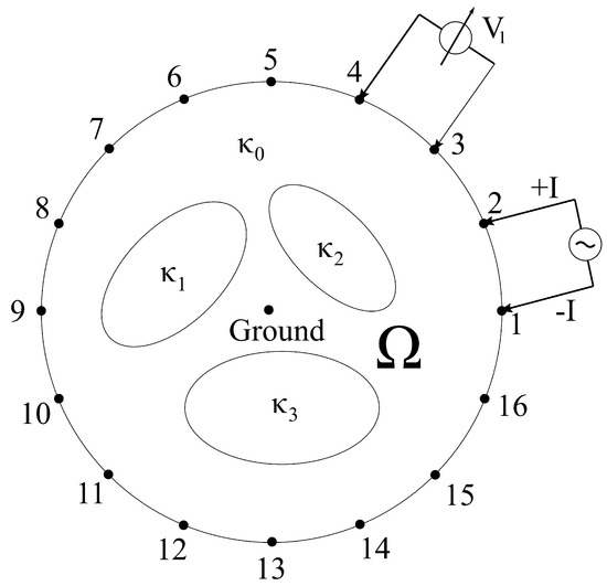 Figure 1. In the implementation of the adjacent pattern (Sheffield method), the numbered electrodes () are placed equidistantly, and the excitation and measurement are performed on adjacent electrodes [1].
 - Then place the generator on the next adjacent pair of electrodes (points 3 and 4 in Figure 1) and take the measurements of the remaining 14 electrodes again.
- All of this is repeated until the generator returns to the starting position [1].
In contrast to these, the system of the equations produced by the LumEM contains conservation equations on the nodes of the resulted graph (Equation (4)). Thus, adopting the numerical method instead of the voltages, it is necessary to consider the potential values; i.e., these values must be recorded during the data collection. Therefore, it is necessary to modify Figure 1 according to the following setup.
According to Figure 2, the generator multiplexing is similar to the classical Sheffield method (with the difference that, instead of electrode in Figure 1, the ground of the system (0 V) is placed). However, in the case of the each generator position, the potential values are measured at the boundary nodes.
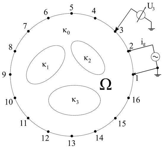
Figure 2.
In the implementation of the modified adjacent pattern, the numbered electrodes () are placed equidistantly, the excitation is performed on adjacent electrodes, and the recorded data consist of potential values.
Hence, in the proposed algorithm, the measurements data are calculated numerically during the solution of the direct problem defined as follows. Letting be a unit disc, and the mathematical problem can be defined as:
where
;
;
;
;
is the ith boundary node ();
n is the number of electrodes (in Figure 2, );
.
The mesh generation is carried out with the help of the Distmesh algorithm [52], as can be seen in Figure 2, by placing fixed nodes at equal distances from each other on the boundary and at the center of the domain. The ground point (0 V) was placed in (this node was deleted from the weighted Laplacian in Equation (4) to obtain the reduced Laplacian), while the excitation was modeled using the Neumann boundary condition. The modified adjacent pattern (Figure 2) utilizes the advantageous properties of the LumEM method, which were successfully validated with FEM by Vizvari et al. [6]. Therefore, the ground point (0 V) and the current generator () represent the two electrodes of the generator connected separately to the adjacent points. Furthermore, the boundary conditions are also prescribed at these points. These two electrodes are meant to create an electric field within the investigated material. The ground point is connected to the boundary point, hence a Dirichlet boundary condition (Equation (5b)) is prescribed at the point. At point , the Neumann boundary condition is defined (Equation (5c)), since a current generator was placed at the point. During the solution of the direct problem, i is changed from 1 to n, as a result of which the positions of Dirichlet (in Equation (5b)) and Neumann (in Equation (5c)) boundary conditions are changed at adjacent nodes.
Equation (4), produced by LumEM, can only be written for a given generator position and excitation signal frequency. If the measurement strategy is applied in detail on a different frequency of the excitation signal, a new system of equations in a form similar to Equation (4) can be written. The significance of the multi-frequency approach lies in the assumption that both the conductivity and the dielectric constant of the material are independent from the excitation frequency in the examined interval. Therefore, only the measured potentials and the admittance () of the material change depend on the frequency. Based on these facts, and as a result of the spectral approach, changing the position of the generator and sweeping the frequency of the excitation signal will not affect the investigated and functions in the model, as only the potential values will change. Taking the advantage of this fact, by applying the spectral approach, the system of equations obtained by formulating the inverse conductivity problem can be overdetermined, which can lead to new possibilities in terms of solvability. By choosing the appropriate measurement frequencies, and by concatenating the system of equations for each data recording procedure, the appropriate system of equations can be constructed, where the number of equations can be calculated as follows:
where
- is number of equations;
- n is number of nodes constructed by LumEM [6];
- is number of frequencies applied for each measurement;
- is number of measurements applied for each generator position.
3.3. The Inverse Problem
With reference to the inverse problem represented by image reconstruction, essentially it is an optimization procedure, where the elements of conductivity (), capacity (), and the potential ( except potentials on boundary) vectors are unknown in Equation (4). The reduced graph branch-node incidence matrix (), the boundary potential values, the angular frequency (), and the excitation current vector () are known. During the solution of the inverse problem, the measurement strategy and method presented in Section 3.1 are applied in the case of a known conductivity function (initial condition). Afterwards, the data collected with the same measurement strategy belonging to , which is considered unknown, are inserted into the system of equations constructed for (this step of the simulation mimics using the measurement data). Thus, the residual of the system of equations formed in this way is no longer zero. Therefore, during the iteration, the residual is minimized in some appropriate norm. Finally, based on initial , the values of vector included in the concatenated system of equations based on the measurement strategy are perturbed with the data belonging to .
Based on the previous explanations and Equation (6), it is obvious how the inverse problem can be overdetermined. If only the data collection strategy at a discrete frequency is considered, it is easy to see that the concatenation of equations written for different generator positions is not sufficient to over-determine the system of equations. The number of unknowns can be calculated as follows:
where
- number of unknown values in the concatenated system;
- number of branches in graph;
- number of nodes placed in domain ().
Based on Equations (6) and (7), overdetermination of the inverse problem can be realized using the properties of the mesh, the number of electrodes, and the measurement strategy. The number of equations (calculated by Equation (6)) can be used to determine how many frequency points are necessary to sweep the measurement spectrally, in order to create an overdetermined inverse problem. Based on the beneficial properties of LumEM, the condition can be satisfied by increasing the number of measurement frequencies. Based on the preliminary measurements, it is recommended to limit the frequency sweep to intervals where both the real and imaginary parts of the function are approximately of the same order of magnitude. This results in a further increase in efficiency and sensitivity.
LumEM transforms the material properties (conductivity and permittivity) into the edges of the resulted graph, and it is defined in the form of weights. These will be the conductivity and capacity values that should be determined during the inverse problem ( terms in Equation (7)) solving. In addition, the potential values obtained during the triangulation at the nodes located inside the domain are still considered unknown ( terms in Equation (7)). This is a consequence of the fact that, during the implementation of the EIT, measurements can only be made on the surface of the investigated material. Therefore, if Equations (6) and (7) are compared, it can be concluded that the number of unknown parameters are independent of the data collection strategy and only depend on the material discretization (graph properties). Now it can be stated that the inverse problem can be overdetermined by choosing the appropriate data collection strategy, since the data collection must be adapted to the already known number of unknowns, where the multi-frequency approach provides great flexibility. Finally, if the modified Sheffield method cannot be used for the collection at a discrete frequency, it is possible to over-determine the problem by repeating it at another frequency. The reason for this is that the unknown conductivity and capacity values on the branches are independent from the frequency.
3.4. Algorithms for Solving Inverse Problems
The concatenated system of the equations is quadratic (non-linear), since the products of the admittance and voltage values interpreted on each branch are displayed. Thus, the following widely-used algorithms can be applied for solving it (even if it is overdetermined): the Newton method, singular value decomposition, and regularization [36,55].
3.4.1. Newton Method
The Newton method is an iterative numerical optimization algorithm that is widely used to find solutions to non-linear systems of equations.
Let and the functions be the elements of the vector . In the case where the system is , the Newton method is defined as follows [36]:
where
- is the solution vector in the step of the iteration;
- is the solution vector in the k step of the iteration;
- is the Moore–Penrose inverse of Jacobian which, due to the quadratic system of equations, can be calculated symbolically as follows:
The advantage of the method lies in the fact (if the Jacobian of the system of equations is invertible) that it can be easily programmed, and the approximation series usually has quadratic convergence [55]. The vector series formed during the iteration converges to the solution of the system of equations. The convergence can be measured in several ways, based on which a stop condition can be defined. For example, in the presented examples, the following stop condition is defined [55]:
where is the user-defined error limit (stop condition) and
3.4.2. Singular Value Decomposition
Here, in the proposed method, the Jacobian cannot be inverted (low rank and/or ill-conditioned), hence the Moore–Penrose inverse is created by using the singular value decomposition of the Jacobian:
where
- is an orthogonal matrix;
- is an orthogonal matrix;
- is an diagonal matrix with non-negative elements that are called singular values.
Based on Equation (12), the generalized inverse of the Jacobian can be obtained as follows:
Since is a diagonal matrix, its inverse is a diagonal matrix as well, where the numbers in the diagonal are reciprocals. Returning to the application of the Newton method, since Jacobian has an inverse in a generalized sense, its Moore–Penrose inverse in Equation (8) can be explicitly expressed [55].
According to the acquired experience [36], due to the small eigenvalues of the Jacobian and measurement errors, the methods mentioned so far are not sufficiently efficient to create a stable optimization procedure that is less sensitive to errors. In the case of the Newton method (Equation (8)), it is necessary to invert the Jacobian; however, only its inverse in the generalized sense can be produced (Equation (13)). Since the Jacobian is ill-conditioned (it lacks rank and has eigenvalues that are very small), the decomposition into singular values does not prove to be an efficient enough solution to produce the Moore–Penrose inverse; therefore, the so-called regularization methods have to be applied. The goal of the regularization is to reduce the effect of small values in , but in such a way as to minimize the information loss. This means that the original problem and its solution are approximated by a problem and its solution, which are less sensitive to errors [55].
3.4.3. Tikhonov Regularization
In this case, to produce the general inverse of the Jacobian, the Tikhonov regularization method [36] is chosen, and its general form is written with the following system of general equations [55]:
where
- is the regularization parameter;
- is the solution vector in case of optimal value;
- is the residual norm;
- is solution seminorm in the case of an prior solution vector.
It is obvious from Equation (14) that the regularization requires that , i.e., the Euclidean norm of the solution, be small (). According to the appropriate literature [55], since in most cases insufficient information about the solution is provided, the start should be (identity matrix) and (zero vector) in Equation (14). Thus, Equation (14) is simplified as follows:
It is obvious from Equation (15) that the goal of Tikhonov’s regularization method is to find a balance between the minimum value of the residual norm (error) and the minimum value of the solution norm. The balance is created by the regularization parameter , hence the choice of an appropriate value is essential during the implementation, in addition to the fact that value of is not trivial at all. The effect of essentially appears during the inversion of in Equation (12). Thus, the reciprocal formation in matrix (in Equation (13)) is corrected with the following “filter function” [56]:
Equation (16) shows that if , then , and if , then . This means that this “filter function” modifies the reciprocal of the eigenvalues and that they vary monotonically between these two extreme values. Thus, in practice, the least amount of information is lost in this case among the methods described so far, while the approximation solution of the system of equations [56] is still produced. The difficulty of applying the method is in the choice of the correct value. This can be implemented, for example, using a graphical method [57]. If the solution norm () vs. residual norm () in the log–log diagram is plotted using different values, the following result will be obtained.
Figure 3 shows that the resulting curve (in the case of ill-posed problems) is always L-shaped, from which it got its name: L-curve. From the L-curve, it can be established that in the case of the optimal value, both the solution norm () and the residual norm () are minimal, i.e., as illustrated by the corner point of the L-curve. The drawback of the iteration algorithm based on the Tikhonov regularization method is that the system of equations must be solved hundreds of times in each iteration step in order to find the optimal value.
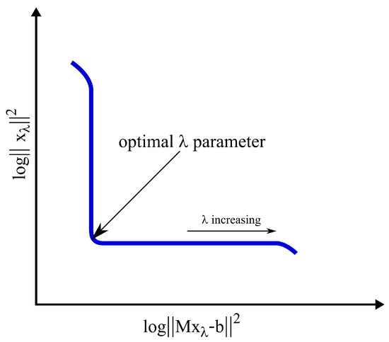
Figure 3.
Diagram of the solution norm () versus residual norm () in the log–log diagram for different values [57].
3.5. Visualization Methods
Since the direct problem is solved in the 2D domain, the functions and are discretized by LumEM. During the discretization, the average and values are obtained at the triangular elements defined by Distmesh. Since the values of conductivity and capacity ( and ) are obtained as a result of the reconstruction appearing on the branches of graph, they can be transformed onto triangles by inverting the transformation described in Equation (2):
where is the Moore–Penrose inverse of the matrix. After applying Equation (17), the values obtained for the triangles are represented by coloring the triangular mesh, taking the advantage of the expression . Therefore, the colored triangular mesh is a straightforward choice for presenting the results.
In order to verify further the effectiveness of the reconstruction, the conductance and capacity values are plotted separately as a function of the branch numbers, with the aim of illustrating the relative error of the reconstruction, which can be calculated as follows:
where
- is the relative error of conductivity value corresponding to the triangle;
- is the relative error of dielectric constant value corresponding to the triangle.
Moreover, since a 2D reconstruction is performed, it is natural to apply 2D visualization tools; therefore, a kernel density estimation (KDE) method is utilized to transform the constant values calculated on the triangles into a surface [58]. Letting and (, ) be the coordinates of triangle centers, then the 2D kernel density estimator applied is defined as follows:
where
is the Epanechnikov kernel function [58], which is placed at the triangle. According to Equation (19), is a 2D function that, smoothed by KDE [58], illustrates the conductivity and permittivity surfaces obtained using the reconstruction, i.e., . During the visualization, is expected to approximate as closely as possible the function defined at the starting point.
4. Reconstruction Algorithm for Inverse Conductivity Problem
The methods described in Section 3 were implemented in a self-developed reconstruction procedure. The first step is to specify the function and generate a triangular mesh using the Distmesh algorithm [52]. Next, by using , the direct problem is solved (based on Section 3.1) using LumEM (Algorithms 1 and 2).
| Algorithm 1: The LumEM solver function. |
 |
Algorithm 1 (LumEM solver function) performs the following tasks:
- The vectors and consist of homogeneous values on the triangles, and they are generated from the functions and by averaging, where the utilized values were taken at the vertices of each triangle and at the center of their circumcircle (row 2 in Algorithm 1) [6].
- Then, Equation (2) calculates the values of the weights (, ) taken on the edges of the graph formed from the triangular mesh. The matrix shown in the input of the procedure is generated using Equation (3). Then, everything is prepared to start calculating the potential values taken at the nodes using Equation (4).
- For this, a “for” loop is started in the first step, where the elements of the angular frequency vector are selected with the k parameter.
- Then another “for” loop starts, which selects the position of the ground point (m in Algorithm 1) on the graph in the case of the modified adjacent pattern shown in Figure 2.
- When applying the LumEM solver function, the following operations are performed for each frequency value and for each generator position:
- (a)
- The vector is created as a null vector, and then the generator current value is entered in the element (rows 6–7 in Algorithm 1);
- (b)
- The column corresponding to the node is deleted from branch-node incidence matrix [6,50], and then the linear equation system is built using the reduced , , matrices, the angular frequency value, and the actually built vector (row 8 in Algorithm 1).
- Obtaining the solution, the equation system provides the potential vector for the entire graph (row 8 in Algorithm 1). Naturally, the previously presented calculation takes place at the generator position and the angular frequency value.
- The resulting data are built from all angular frequency values and n generator positions. This structure is defined as a solution to the direct problem.
The LumEM solver function (Algorithm 1) is used during the implementation of the direct solver procedure described in Algorithm 2. The inputs for solving the direct problem are the number of electrodes (n), the data from the mesh generated by Delunay triangulation, the and functions, the angular frequency vector, and the value of the generator current .
| Algorithm 2: Direct problem solver. |
| Input: n, mesh data, , , , |
| Output: , , |
| 1 build from mesh data |
| 2 build from mesh data (Equation (3)) |
| 3 , , = LumEM Solver(n, , , , , , ) |
| 4 = |
The direct problem solver procedure works as follows:
- In the first step, the solver calculates the branch-node incidence matrix.
- In the second step (based on Equation (4)), the transformation matrix is constructed.
- Then, using these matrices and all the other input parameters, the LumEM solver function is run, which generates the , matrices and the potential data structure.
- For further calculations, the values taken from the data are only needed at boundary nodes; therefore, during the generation of the structure, these are extracted from the dataset. Thus, the structure only contains values taken at the boundary nodes for all generator positions and angular frequencies.
The most important input data for the reconstruction are the data collected using the modified adjacent pattern method explained in detail in Section 3.2. The solution for the direct problem (implemented by Algorithm 2), more precisely the implementation of LumEM, also needs a mesh generation procedure, which is one of the key steps of the algorithm, since the mesh generated by Distmesh [52] is used in all subsequent steps of the reconstruction. It is very important to emphasize that, for the further calculations, it is necessary to use the same mesh, and the same measurement strategy is also a necessary condition for the application of the method described in Algorithm 3. After the basic data of the reconstruction have been produced, a system of linear equations corresponding to the initial conditions of the inverse procedure is defined. This actually means the solving of an another direct problem, now using the initial condition (Algorithm 3). In this case, the applied measurement strategy, the LumEM discretization, and the function representing the initial condition can be used to generate the system of equations (in the form of Equation (4)) required to solve the inverse problem.
The steps in Algorithm 3 are as follows:
- The handling of the initial condition is fully consistent with the procedure described in Algorithm 2, since the LumEM solver function (Algorithm 1) is used in the same way. However, in this case, the , matrices are calculated from the function (row 3 in Algorithm 3).
- Nevertheless, here the potential structure is not extracted for boundary vertices only, as it is extracted for all the other nodes too.
- After these steps, and before starting the Newton iteration, the vector is generated by rearranging and concatenating the , and structures.
- Entering the Newton iteration (after step ), and are extracted from the vector (rows 7–9 in Algorithm 3).
- Then, two “for” loops are started, where angular frequencies are selected by k and generator positions are parameterized by m (rows 10–11 in Algorithm 3).
- The generator vector is handled in exactly the same way as in the case of the LumEM solver function (Algorithm 1).
- Next, the potential vector for the actual angular frequency and generator position is extracted from the vector.
- The driving force of the reconstruction algorithm comes from the fact that the calculated from function and taken from boundary points is concatenated with , calculated from the , rather than taken at non-boundary points at all present frequencies and generator positions (row 15 in Algorithm 3).
- The residual of the equation system (calculated from the potential vector , matrices , , , the current angular frequency value, and the vector) is no longer zero in Algorithm 3 (row 16 in Algorithm 3).
- At each angular frequency value and generator position (and naturally, at each step in the Newton iteration (Section 3.4.1)), a new and updated Jacobian matrix is applied. The Jacobian matrix (based on Section 3.4.1) can be determined by simple derivation, since now the represents a system of quadratic equations.
- The generalized inverse Jacobian required for the method is approximated using SVD (Section 3.4.2) [55] and Tikhonov regularization (Section 3.4.3) [55] in each step of the iteration (at each angular frequency value and generator position). The optimal parameter, based on the L-curve (Figure 3) [57], is generated using the MATLAB Regularization Toolbox at each step of the iteration (rows 18–19 in Algorithm 3) [57].
- As the product of the residual vector and the generalized inverse of the Jacobian at the actual angular frequency and generator position, the vector is calculated and then concatenated to all elements of the frequency vector and the generator position into a general vector.
- Next, a Newton step [36] is performed by (row 24 in Algorithm 3).
- The Newton iteration continues until the defined stop condition is achieved. The value of the stop condition is defined as one of the inputs in Algorithm 3. Actually, this is how the solution method of the quadratic system of equations (considering the unknown , matrices and vectors) is implemented in Algorithm 3. This system is an overdetermined system of equations, where the number of equations can be calculated using Equation (6), while the number of unknowns can be calculated using Equation (7).
- After the optimal solution is determined, the and vectors are extraxted from and transformed into and vectors using Equation (17) (rows 27–30 in Algorithm 3).
In order to be able to visually display the result of the reconstruction by the KDE method (described in Section 3.5), the surface for this purpose can be created on an appropriately high-resolution mesh grid.
Regarding the computational cost of the entire solution procedure, the dominant operation is the calculation of the singular value decomposition of the Jacobian (Section 3.4.2). Since the economy-size decomposition of the built in MATLAB implementation is used, the computational complexity for the Jacobian is . The computational cost solely relies on the complexity of this operation; everything else is practically negligible compared to it.
| Algorithm 3: Inverse problem solver. |
 |
5. Case Studies
The case studies and the algorithms needed for the solution were implemented in the MATLAB environment. In the case studies, the reconstruction of the function shown in Figure 4 was performed.
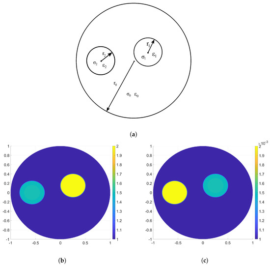
Figure 4.
function used for case studies, (a) applied domain for case studies, (, , , , , , , , , , , , , , ); (b) the applied function; (c) the applied function.
As can be seen in Figure 4a, the 2D domain is actually a unit circle (, , ) where, as the background, the and functions are chosen. Inside the unit circle, two sub-domains are defined with the following properties (Figure 4a):
To solve the case studies, three different triangular meshes (Figure 5) were generated using the Distmesh algorithm [52]:
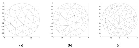
Figure 5.
The applied meshes used for case studies, (a) triangular mesh with 16 electrodes (, , , ), (b) triangular mesh with 24 electrodes (, , , ), (c) triangular mesh with 32 electrodes (, , , ).
- Triangular mesh with 16 electrodes: , , , ;
- Triangular mesh with 24 electrodes: , , , ;
- Triangular mesh with 32 electrodes: , , , .
The and values discretized using LumEM (Section 3.1) are shown in the following figure (Figure 6):
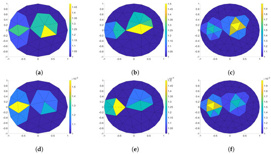
Figure 6.
The discretized and values; values for (a) 16, (b) 24, (c) 32 electrodes; values for (d) 16, (e) 24, (f) 32 electrodes.
By applying Algorithm 2, the direct problem was solved in all three cases. The value of in all three cases was , while the angular frequency vector used was . The initial conditions for the inverse problem-solving procedure (Algorithm 3) are the same and functions (in the whole domain) for all three triangular meshes. The stopping condition for all three calculations was . The data of the equation systems generated from the initial values during the inverse problem are as follows (based on Equations (6) and (7)):
The length and elements of the vector were chosen to be applied universally for all three meshes, without any changes. The frequency values were selected empirically based on the knowledge of and , ensuring that the real part and the imaginary part of at each frequency point were approximately of the same order of magnitude. This is the method by which the maximum sensitivity can be achieved in the case studies, by means of a properly planned data collection strategy.
The inverse problem solving procedure converged in all three cases in 13, 10, and 18 steps for the cases with 16, 24, and 32 electrodes, respectively. The relative error values calculated with Equation (18) for each triangle are shown in Figure 7.
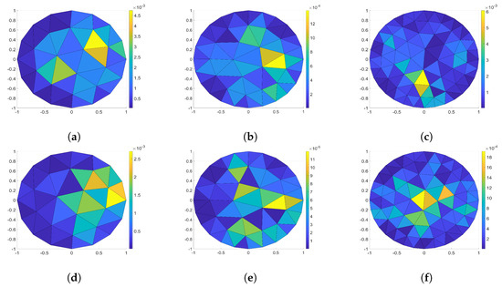
Figure 7.
The spatial distribution of the relative error calculated using Equation (18) for each triangle; (a) for 16, (b) for 24, (c) for 32 electrodes, (d) for 16, (e) for 24, (f) for 32 electrodes.
Nothing shows the success of all three reconstructions better than the fact that the relative error values remained below in all cases (Figure 7). Based on Figure 6d and Figure 7a:
- The maximum relative error values of the 16-electrode solution were and ;
- For the 24-electrode solution, they were and ;
- For the 32-electrode solution, they were , and .
Next, the KDE visualization (based on Equation (19)) provides the following results shown in Figure 8:
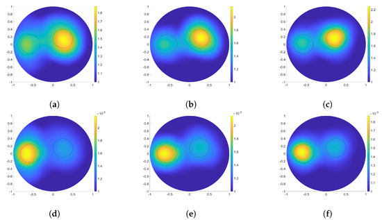
Figure 8.
KDE-based visualization of reconstruction results based on Equation (19), for (a) 16, (b) 24, (c) 32 electrodes, for (d) 16, (e) 24, (f) 32 electrodes.
6. Conclusions
In this paper, a new approach to EIT image reconstruction was proposed. The procedure was based on a new numerical approach, the Lumped Element Method (LumEM), which was developed and presented. A major advantage of the numerical procedure developed in this research is the discretization procedure implementation of the conductivity and dielectric constant functions using a triangular mesh, with the discretization of the investigated domain. As a result, a linear system of equations was obtained that enforces the symmetry of the original differential operator and the local conservation principles in addition to the global conservation principles. Furthermore, these beneficial properties are significant in the use of inverse problem determination. Additionally, the application of the proposed procedure and the multi-frequency approach led to an overdetermined system of quadratic equations, which needs to be solved during the image reconstruction. The Jacobian of the system can be defined symbolically and updated at each step of the iteration by simple substitution. Due to the ill-posed nature of the problem, it is necessary to utilize the Tikhonov regularization (Section 3.4.3) in the iteration steps of the Newton-method-based minimization procedure (Section 3.4.1).
In order to illustrate all the advantages of the developed method, case studies were examined and presented. Based on them, it can be concluded that the inverse problem solving and reconstruction procedure was effectively able to restore the constant conductivity and constant dielectric values assigned to the triangular mesh. Despite the fact that the relative error values remain below 1%, the reconstructed values cannot be directly used to produce interpretable images. Therefore, a KDE-based imaging procedure was presented, which can be used to create 2D surfaces from the reconstructed values. Since this research focuses only on the reconstruction, the parameterization of the KDE was done empirically, as the goal was only to display the results of the reconstruction. In current case studies with coarse mesh resolution, it is obvious that the LumEM-based inverse procedure is effective in the localization of the inhomogeneities placed in conductivity and dielectric constant functions.
7. Future Work
The imaging part is the most important milestone for the future; in addition to the further development of KDE, the goal is to implement and apply several methods (for example, image processing methods such as upsampling or super resolution image reconstruction methods, etc.). Moreover, effective localization is necessary, as it is still not a sufficient condition for technical applications. Furthermore, it is necessary to improve the sensitivity of the method by improving the shape recognition. By creating and applying new symmetric measurement strategies, it is possible to examine which useful properties can be used to increase the effectiveness. For this purpose, based on the existing and well-described methods in the literature, it is possible to develop new methods that maximally exploit the beneficial properties of the LumEM method.
Author Contributions
Z.S. drafted the manuscript and conceived and performed the experiments. M.K., P.O. and Z.V. checked the test results and suggested the corrections. V.T. and A.T. supervised the research and contributed to the organization of article. All authors have read and agreed to the published version of the manuscript.
Funding
This research received no external funding.
Institutional Review Board Statement
Not applicable.
Informed Consent Statement
Not applicable.
Data Availability Statement
Not applicable.
Acknowledgments
The publication was granted by the Faculty of Engineering at University of Pécs, Hungary, within the framework of the ‘Call for Grant for Publication (2.0)’. The authors would like to thank the editors and the anonymous reviewers for their valuable comments that significantly improved the quality of this paper.
Conflicts of Interest
The authors declare no conflict of interest.
References
- Holder, D. Electrical Impedance Tomography: Methods, History, and Applications; Institute of Physics Pub: Bristol, PA, USA, 2005; ISBN 9780750309523. [Google Scholar]
- Amalia, I. Continuous and Discrete Simulation in Electrodynamics; Akademiai Kiado: Budapest, Hungary, 2003; ISBN 9630579987. (In Hungarian) [Google Scholar]
- Cardoso, J. Electromagnetics through the Finite Element Method: A Simplified Approach Using Maxwell’s Equations; CRC Press: Boca Raton, FL, USA; Taylor & Francis Group: Oxfordshire, UK, 2017; ISBN 1498783570. [Google Scholar]
- Jin, J.M. The Finite Element Method in Electromagnetics, 3rd ed.; John Wiley and Sons: Hoboken, NJ, USA, 2014; ISBN 1118571363. [Google Scholar]
- Calderón, A.P. On an inverse boundary value problem. Comput. Appl. Math. Braz. Soc. Comput. Appl. Math. (SBMAC) 2006, 25, 2–3. [Google Scholar] [CrossRef]
- Vizvari, Z.; Klincsik, M.; Sari, Z.; Odry, P. Lumped Element Method—A Discrete Calculus Approach for Solving Elliptic and Parabolic PDEs. Acta Polytech. Hung. 2021, 18, 201–223. [Google Scholar] [CrossRef]
- Uhlmann, G. 30 Years of Calderón’s Problem, Seminaire Laurent Schwartz—EDP et Applications, Cellule MathDoc/CEDRAM, 2012, Séminaire Laurent Schwartz—EDP et Applications, 1–25. Available online: https://slsedp.centre-mersenne.org/item/SLSEDP_2012-2013____A13_0/ (accessed on 27 April 2023).
- Uhlmann, G. Electrical Impedance Tomography and Calderón’s Problem. Inverse Probl. 2009, 25, 123011. [Google Scholar] [CrossRef]
- Siltanen, S.; Mueller, J.L.; Isaacson, D. Reconstruction of high contrast 2-D conductivities by the algorithm of A. Nachman. Am. Math. Soc. 2001, 278, 241–254. [Google Scholar]
- Mueller, J.; Siltanen, S.; Isaacson, D. A direct reconstruction algorithm for electrical impedance tomography. IEEE Trans. Med Imaging Inst. Electr. Electron. Eng. 2002, 21, 555–559. [Google Scholar] [CrossRef] [PubMed]
- Li, T.; Isaacson, D.; Newell, J.C.; Saulnier, G.J. Studies of an Adaptive Kaczmarz Method for Electrical Impedance Imaging. J. Physics: Conf. Ser. 2013, 434, 012075. [Google Scholar] [CrossRef]
- Li, T.; Kao, T.J.; Isaacson, D.; Newell, J.C.; Saulnier, G.J. Adaptive Kaczmarz Method for Image Reconstruction in Electrical Impedance Tomography. Physiol. Meas. 2013, 34, 595–608. [Google Scholar] [CrossRef]
- Chen, Z.Q. Reconstruction Algorithms for Electrical Impedance Tomography. Ph.D. Thesis, Department of Electrical and Computer Engineering, University of Wollongong, Hong Kong, China, 1990. Available online: http://ro.uow.edu.au/theses/1348 (accessed on 29 March 2023).
- Ahn, S.; Oh, T.I.; Jun, S.C.; Seo, J.K.; Woo, J.E.J. Validation of Weighted Frequency-Difference EIT Using a Three-Dimensional Hemisphere Model and Phantom. Physiol. Meas. 2011, 32, 1663–1680. [Google Scholar] [CrossRef] [PubMed]
- Boverman, G.; Isaacson, D.; Newell, J.C.; Saulnier, G.J.; Kao, T.J.; Amm, B.C.; Wang, X.; Davenport, D.; Chong, D.H.; Sahni, R.; et al. Efficient Simultaneous Reconstruction of Time-Varying Images and Electrode Contact Impedances in Electrical Impedance Tomography. IEEE Trans. Biomed. Eng. Inst. Electr. Electron. Eng. 2017, 64, 795–806. [Google Scholar] [CrossRef] [PubMed]
- Jerbi, K.; Lionheart, W.R.B.; Vauhkonen, P.J.; Vauhkonen, M. Sensitivity matrix and reconstruction algorithm for EIT assuming axial uniformity. Physiol. Meas. 2000, 21, 61–66. [Google Scholar] [CrossRef]
- Lionheart, W.R. Reconstruction Algorithms for Permittivity and Conductivity Imaging. In Proceedings of the 2nd World Congress on Industrial Process Tomography, Hannover, Germany, 29–31 August 2001; pp. 4–11. [Google Scholar]
- Graham, B.M.; Adler, A. Electrode placement configurations for 3D EIT. Physiol. Meas. 2007, 28, S29–S44. [Google Scholar] [CrossRef] [PubMed]
- Paridis, K.; Lionheart, W.R.B. Shape corrections for 3D EIT. J. Phys. Conf. Ser. 2010, 224, 012049. [Google Scholar] [CrossRef]
- Polydorides, N. Image Reconstruction Algorithms for Soft-Field Tomography. Ph.D. Thesis, University of Manchester Institute of Science and Technology, Manchester, UK, 2002. [Google Scholar]
- Akhtari-Zavare, M.; Latiff, L.A. Electrical Impedance Tomography as a Primary Screening Technique for Breast Cancer Detection, Asian Pacific Journal of Cancer Prevention. Asian Pac. Organ. Cancer Prev. 2015, 16, 5595–5597. [Google Scholar] [CrossRef] [PubMed]
- Karpov, A.; Korotkova, M.; Shiferson, G.; Kotomina, E. Electrical Impedance Mammography: Screening and Basic Principles, Breast Cancer and Breast Reconstruction; IntechOpen: London, UK, 2020; Available online: https://www.intechopen.com/chapters/69046 (accessed on 29 March 2023). [CrossRef]
- Spatenkova, V.; Teschner, E.; Jedlicka, J. Evaluation of regional ventilation by electric impedance tomography during percutaneous dilatational tracheostomy in neurocritical care: A pilot study. BMC Neurol. 2020, 20, 374. [Google Scholar] [CrossRef]
- Zhang, N.; Jiang, H.; Zhang, C.; Li, Q.; Li, Y.; Zhang, B.; Deng, J.; Niu, G.; Yang, B.; Frerichs, I.; et al. The influence of an electrical impedance tomography belt on lung function determined by spirometry in sitting position. Physiol. Meas. 2020, 41, 044002. [Google Scholar] [CrossRef]
- Luo, Y.; Abiri, P.; Chang, C.C.; Tai, Y.C.; Hsiai, T.K. Epidermal EIT Electrode Arrays for Cardiopulmonary Application and Fatty Liver Infiltration. Interfacing Bioelectron. Biomed. Sens. 2020, 163–184. [Google Scholar]
- Humplik, P.; Cermak, P.; Zid, T. Electrical impedance tomography for decay diagnostics of Norway spruce (Picea abies): Possibilities and opportunities. Silva Fenn. Finn. Soc. For. Sci. 2016, 50, 1341. [Google Scholar] [CrossRef]
- Proto, A.R.; Cataldo, M.F.; Costa, C.; Papandrea, S.F.; Zimbalatti, G. A tomographic approach to assessing the possibility of ring shake presence in standing chestnut trees. Eur. J. Wood Wood Prod. 2020, 78, 1137–1148. [Google Scholar] [CrossRef]
- Hong, L.E.; Yunos, Y.B.M. Application of FPGA in Process Tomography Systems. Engineering 2020, 12, 790–809. [Google Scholar] [CrossRef]
- Sahovic, B.; Atmani, H.; Sattar, M.A.; Garcia, M.M.; Schleicher, E.; Legendre, D.; Climent, E.; Zamansky, R.; Pedrono, A.; Babout, L.; et al. Controlled Inline Fluid Separation Based on Smart Process Tomography Sensors. Chem. Ing. Tech. 2020, 92, 554–563. [Google Scholar] [CrossRef]
- Boyle, A. Geophysical Applications of Electrical Impedance Tomography. Ph.D. Thesis, Carleton University, Ottawa, ON, Canada, 2016. [Google Scholar]
- Molyneux, J.E.; Witten, A. Impedance tomography: Imaging algorithms for geophysical applications. Inverse Probl. 1994, 10, 655–667. [Google Scholar] [CrossRef]
- Beilina, L.; Klibanov, M.V. A posteriori error estimates for the adaptivity technique for the Tikhonov functional and global convergence for a coefficient inverse problem. Inverse Probl. 2010, 26, 045012. [Google Scholar] [CrossRef]
- Beilina, L.; Klibanov, M.V. Reconstruction of dielectrics from experimental data via a hybrid globally convergent/adaptive inverse algorithm. Inverse Probl. 2010, 26, 125009. [Google Scholar] [CrossRef]
- Beilina, L.; Klibanov, M.V. Approximate Global Convergence and Adaptivity for Coefficient Inverse Problems. Springer: New York, NY, USA, 2010; ISBN 9781441978059. [Google Scholar]
- Mueller, J.L.; Siltanen, S. Linear and Nonlinear Inverse Problems with Practical Applications; SIAM: Philadelphia, PA, USA, 2012; ISBN 9781611972337. [Google Scholar]
- Isakov, V. Inverse Problems for Partial Differential Equations; Springer International Publishing: Berlin/Heidelberg, Germany, 2017; ISBN 9783319516578. [Google Scholar]
- Koyunbakan, H. Inverse nodal problem for p-Laplacian energy-dependent Sturm-Liouville equation. Bound. Value Probl. 2013, 2013, 272. [Google Scholar] [CrossRef]
- Koyunbakan, H. Reconstruction of Potential in Discrete Sturm–Liouville Problem. Qual. Theory Dyn. Syst. 2022, 21, 13. [Google Scholar] [CrossRef]
- Khaled, D.E.; Novas, N.; Gazquez, J.A.; Manzano-Agugliaro, F. Dielectric and Bioimpedance Research Studies: A Scientometric Approach Using the Scopus Database. Publications 2018, 6, 6. [Google Scholar] [CrossRef]
- Naranjo-Hernández, D.; Reina-Tosina, J.; Min, M. Fundamentals, Recent Advances, and Future Challenges in Bioimpedance Devices for Healthcare Applications. J. Sens. 2019, 2019, 9210258. [Google Scholar] [CrossRef]
- Liu, D.; Wang, J.; Shan, Q.; Smyl, D.; Deng, J.; Du, J. DeepEIT: Deep Image Prior Enabled Electrical Impedance Tomography. IEEE Trans. Pattern Anal. Mach. Intell. 2023, 1–12. [Google Scholar] [CrossRef]
- Wang, W.; Yousaf, M.; Liu, D.; Sohail, A. A Comparative Study of the Genetic Deep Learning Image Segmentation Algorithms. Symmetry 2022, 14, 1977. [Google Scholar] [CrossRef]
- Colibazzi, F.; Lazzaro, D.; Morigi, S.; Samore, A. Learning Nonlinear Electrical Impedance Tomography. J. Sci. Comput. 2022, 90, 58. [Google Scholar] [CrossRef]
- Wang, G.; Feng, D.; Tang, W. Electrical Impedance Tomography Based on Grey Wolf Optimized Radial Basis Function Neural Network. Micromachines 2022, 13, 1120. [Google Scholar] [CrossRef] [PubMed]
- Bibi, K. Particular Solutions of Ordinary Differential Equations Using Discrete Symmetry Groups. Symmetry 2020, 12, 180. [Google Scholar] [CrossRef]
- Jauhiainen, J.; Seppänen, A.; Valkonen, T. Mumford–Shah regularization in electrical impedance tomography with complete electrode model. Inverse Probl. 2022, 38, 065004. [Google Scholar] [CrossRef]
- Chen, Z.; Xiang, J.; PBagnaninchi, P.-O.; Yang, Y. MMV-Net: A Multiple Measurement Vector Network for Multifrequency Electrical Impedance Tomography. IEEE Trans. Neural Netw. Learn. Syst. 2022, 1–12. [Google Scholar] [CrossRef] [PubMed]
- Benoit, B.; Yassine, H.; Nabil, Z. Robust imaging using electrical impedance tomography: Review of current tools. Proc. R. Soc. Math. Phys. Eng. Sci. 2022, 478, 2258. [Google Scholar]
- Perot, J.; Subramanian, V. Discrete calculus methods for diffusion. J. Comput. Phys. 2007, 224, 59–81. [Google Scholar] [CrossRef]
- Leo, J.; Grady, J.P. Discrete Calculus; Springer: London, UK, 2010; ISBN 1849962898. [Google Scholar]
- Subramanian, V. Discrete Calculus Methods and Their Implementation. Ph.D. Thesis, Mechanical Engineering, University of Massachusetts, Amherst, MA, USA, 2007. [Google Scholar]
- Persson, P.O.; Strang, G. A Simple Mesh Generator in MATLAB. Siam Rev. Soc. Ind. Appl. Math. (SIAM) 2004, 46, 329–345. [Google Scholar] [CrossRef]
- Alhevaz, A.; Baghipur, M.; Ganie, H.A.; Shang, Y. Bounds for the Generalized Distance Eigenvalues of a Graph. Symmetry 2019, 11, 1529. [Google Scholar] [CrossRef]
- Garde, H.; Hyvönen, N. Mimicking relative continuum measurements by electrode data in two-dimensional electrical impedance tomography. Numer. Math. 2021, 147, 579–609. [Google Scholar] [CrossRef]
- Aster, R.; Borchers, B.; Thurber, C.H. Parameter Estimation and Inverse Problems; Elsevier Academic Press: Amsterdam, The Netherlands, 2005; ISBN 9780080470559. [Google Scholar]
- Hanka, L. An efficient quadratic programming optimization method for deconvolution of gamma-ray spectra. AARMS Technol. 2010, 9, 47–66. [Google Scholar]
- Hansen, P.C. Regularization Tools Version 4.0 for Matlab 7.3. Numer. Algorithms 2007, 46, 189–194. [Google Scholar] [CrossRef]
- Gramacki, A. Nonparametric Kernel Density Estimation and Its Computational Aspects; Springer: Cham, Switzerland, 2018; ISBN 9783319716879. [Google Scholar]


Disclaimer/Publisher’s Note: The statements, opinions and data contained in all publications are solely those of the individual author(s) and contributor(s) and not of MDPI and/or the editor(s). MDPI and/or the editor(s) disclaim responsibility for any injury to people or property resulting from any ideas, methods, instructions or products referred to in the content. |
© 2023 by the authors. Licensee MDPI, Basel, Switzerland. This article is an open access article distributed under the terms and conditions of the Creative Commons Attribution (CC BY) license (https://creativecommons.org/licenses/by/4.0/).