Galerkin Method for a Backward Problem of Time-Space Fractional Symmetric Diffusion Equation

Abstract

We investigate a backward problem of the time-space fractional symmetric diffusion equation with a source term, wherein the negative Laplace operator $-\Delta$ contained in the main equation belongs to the category of uniformly symmetric elliptic operators. The problem is ill-posed because the solution does not depend continuously on the measured data. In this paper, the existence and uniqueness of the solution and the conditional stability for the inverse problem are given and proven. Based on the least squares technique, we construct a Galerkin regularization method to overcome the ill-posedness of the considered problem. Under a priori and a posteriori selection rules for the regularization parameter, the Hölder-type convergence results of optimal order for the proposed method are derived. Meanwhile, we verify the regularized effect of our method by carrying out some numerical experiments where the initial value function is a smooth function or a non-smooth one. Numerical results show that this method works well in dealing with the backward problem of the time-space fractional parabolic equation.

1. Introduction

In the fields of thermodynamics and biology, classical integer order parabolic equations are used to describe normal diffusion phenomena. However, with the development of technology and driven by the in-depth study of some practical scientific problems, people find that more and more abnormal diffusion phenomena appear in the real world, such as the diffusion problems that occur in some medias with memory and genetic characteristics. For this reason, with the help of fractional calculus theories and methods, mathematicians and physicists have derived various time or space fractional parabolic equations. Here, the time fractional derivative in a fractional parabolic equation can be used to describe particle sticking and trapping phenomena, and the space fractional derivative usually describes the long particle jump. In the past few decades, the direct problems of fractional parabolic equations have attracted more and more attention, and fractional calculus has been used in many scientific fields, such as bioengineering, pharmacokinetics, tissue dynamics, economic, and epidemiology [1,2,3,4]. In recent years, in view of the requirement of dealing with some practical problems, more and more people are focusing on the inverse problems of fractional parabolic equations, which mainly include the inverse source problem [5], parameter identification problem [6], sideways problem [7], backward problem in time (inverse initial value problem or final value problem) [8], etc.

In the present paper, we consider the backward problem of the time-space fractional parabolic equation:

$$\begin{array}{c}\hfill \left\{\begin{array}{c}\frac{{\partial }^{\alpha }u(x,t)}{\partial t^{\alpha }}+{(-\Delta )}^{\frac{\beta }{2}}u(x,t)=f(x,t),x\in \Omega ,0<t<T,\hfill \\ u(x,t)=0,x\in \partial \Omega ,0<t<T,\hfill \\ u(x,T)=g\left(x\right),x\in \Omega ,\hfill \end{array}\right.\end{array}$$

(1)

where $\Omega :(-1,1)$, $T>0$ is a fixed final time, and $\alpha \in (0,1)$ and $\beta \in (1,2)$ are fractional orders of the time and space derivatives, respectively. The fractional derivative $\frac{{\partial }^{\alpha }u}{\partial t^{\alpha }}$ denotes the Caputo fractional derivative about the time variable of the function $u(x,t)$, which is defined as [9]:

$$\begin{array}{c}\hfill \frac{{\partial }^{\alpha }u}{\partial t^{\alpha }}=\frac{1}{\Gamma (1-\alpha )}{\int }_0^t\frac{\partial u(x,s)}{\partial s}\frac{ds}{{(t-s)}^{\alpha }},0<\alpha <1,\end{array}$$

(2)

$$\begin{array}{c}\hfill \frac{{\partial }^{\alpha }u}{\partial t^{\alpha }}=\frac{\partial u(x,t)}{\partial t},\alpha =1,\end{array}$$

(3)

and $\Gamma (·)$ is the Gamma function. The fractional Laplacian operator ${(-\Delta )}^{\frac{\beta }{2}}$ of order $\beta (1<\beta <2)$ is defined by using the spectral decomposition of the Laplace operator. The definition is summarized in Section 2; also see [10]. $g\left(x\right)\in L^2(\Omega )$ is the exact final value data, and $f(x,t)\in L^{\infty }(0,T;L^2(\Omega ))$ denotes the source term. Let $\delta >0$ be the bound of the measured error, denoting $g^{\delta }\left(x\right)$ and $f^{\delta }(x,t)$ as the noisy final value and source term data, respectively, which satisfy:

$$\begin{array}{c}\hfill {∥g^{\delta }\left(x\right)-g\left(x\right)∥}_{L^2(\Omega )}\le \delta ,\end{array}$$

(4)

$$\begin{array}{c}\hfill {∥f^{\delta }(x,t)-f(x,t)∥}_{L^{\infty }(0,T;L^2(\Omega ))}\le \delta .\end{array}$$

(5)

Our task is to determine the initial value $u(x,0)$ from the noisy datum $g^{\delta }\left(x\right)$ and $f^{\delta }(x,t)$.

Note that, when $\alpha =1$, $\beta =2$, the governing equation of (1) is the classical diffusion equation, this equation is usually used to describe the normal diffusion phenomenon, and in the normal diffusion process the diffusion flux follows Fick’s law. In physics and biology, the classical diffusion equation is also used to describe the density distribution of particles in Brownian motion. When $0<\alpha <1$, $\beta =2$, the governing equation of (1) is called the time-fractional diffusion equation, which can be used to describe some anomalous diffusion phenomena. This is because many anomalous diffusions do not follow Fick’s law, but rather follow the time-fractional Fick’s law in natural science. In physics and biology, the time-fractional diffusion equation is also used to describe the density distribution of particles in fractional Brownian motion. When $\alpha =1$, $1<\beta <2$, the governing equation of (1) is called the space-fractional diffusion equation. This equation often describes the diffusion law of particles driven by a Lévy flights. When $0<\alpha <1$, $1<\beta <2$, as is the case in this paper, the governing equation of (1) can be used to describe the diffusion law of particles that simultaneously follow the Lévy and fractional Brownian processes; see [11,12].

We know that the backward problem of the time-fractional parabolic equation $(0<\alpha <1,\beta =2)$ has been studied by many researchers, and some meaningful regularization methods have been presented and used to overcome the ill-posedness—for instance, the quasi-reversible method [13,14], total variation method [15], iterative fractional Tikhonov method [16], projection method [17], truncation method [18], simplified Tikhonov method [19], and fractional Tikhonov method [20]. For the backward problem of the space-fractional parabolic equation $(\alpha =1,1<\beta <2)$, there also have been some research works in which some regularization methods have been developed, such as the convolution and spectral methods [21], iteration method [22], simplified Tikhonov method [23], the logarithmic, negative exponential and fractional Tikhonov methods [24,25,26], optimal method [27], modified kernel method [28], and generalized Tikhonov method [29]. For the backward problem of the time-space fractional parabolic equation, some works have recently been published, in which some interesting and efficient regularization methods have been proposed—for instance, the fundamental kernel-based method [30], variable total variation method [31], modified iterated Lavrentiev method [32], fractional Tikhonov method [33,34], quasi-boundary value method [35], modified Tikhonov method [36], and modified quasi-boundary value method [37].

Followed on the above existing works, this paper continues to consider the backward problem (1). There are many examples of abnormal diffusion in Physics, such as the diffusion of pollen or haze. In the diffusion process, we only know the solute concentration in a certain position at the current moment. However, we often hope to know the solute concentration at the initial time. The above problem can be transformed into the solution of the backward problem of time-space fractional diffusion Equation (1), which is an ill-posed problem. Based on the ill-posedness analysis, the results of the existence and the uniqueness of the solution and conditional stability are given and proven. Then, we construct a Galerkin regularization method based on the least squares technique to recover the stability of the solution and apply it to solve the backward problem of the time-space fractional diffusion equation. Meanwhile, with the help of the conditional stability result, the Hölder-type a priori and a posteriori convergence results for the regularization method are derived. Finally, we solve a forward problem to construct the exact datum, and compute the exact and regularized solutions through respective analytic expression. The simulation effects of the regularization method are also verified by carrying out some numerical experiments.

The Galerkin method is an excellent numerical calculation method, because it has an approximate space composed of discontinuous piecewise functions. These discontinuities occur at the boundaries of the partitioning elements, and these are continuous inside the partitioning elements. Therefore, this method is often used to solve the problems faced in the finite element method; see [38]. Recently, various Galerkin methods have been developed and used in some fields of inverse problems. For instance, Ref. [39] presented and used a local discontinuous Galerkin method to identify the space-dependent source term in a time-fractional diffusion equation. In [40], the authors used the local discontinuous Galerkin method to research a time-fractional diffusion inverse problem subject to an extra measurement. Ref. [41] constructed a spectral Galerkin method to solve a Cauchy problem of the Helmholtz equation. For other works related to this type of method, please see [42,43], etc. The method in this paper is a discrete regularization one. The basic idea of this method is: under the action of orthogonal projection, we can transform an ill-posed operator equation in infinite dimensional space into a linear system in finite dimensional subspace, and construct the regularization solution of the original inverse problem with the help of the least squares technique. Here, the dimension of the finite dimensional subspace plays the role of the regularization parameter. From the numerical algorithm perspective, this method has low computational complexity, and it is easy to be implemented. In addition, the Galerkin method has the convergence property of high order in the sense of weak norms, and there are also many applications in some specific problems, such as the boundary element methods for solving boundary value problems. On the general theory of the discrete regularization method, we can refer to [44,45], and so on.

The rest of this article is arranged as follows. In Section 2, we present some preparatory knowledge. Section 3 presents and proves the results of existence and uniqueness, as well as the conditional stability for te inverse problem. Section 4 describes the construction procedure of the regularized method. Section 5 derives a priori and a posteriori convergence results of the regularization method. In Section 6, we verify the simulation effect of our method by performing some numerical experiments. Some conclusions and discussions are presented in Section 7.

2. Preliminary Knowledge

We first need a few properties of the eigenvalues of the negative Laplace operator $-\Delta$; please see [9,46], etc.

Proposition 1. 

1. Denote the eigenvalues of $-\Delta$ as ${\overline{\lambda }}_k(k=1,2,···)$, and suppose that $0<{\overline{\lambda }}_1\le {\overline{\lambda }}_2\le ···\le {\overline{\lambda }}_k\le ···$, and ${\overline{\lambda }}_k\to \infty$ as $k\to \infty$. 2. Let ${\left\{w_k\left(x\right)\right\}}_{k=1}^{\infty }$ be the corresponding eigenfunctions; thus, $({\overline{\lambda }}_k,w_k\left(x\right))$ satisfy the boundary value problem:

$$\begin{array}{c}\hfill \left\{\begin{array}{c}-\Delta w_k\left(x\right)={\overline{\lambda }}_k{w}_k\left(x\right),x\in \Omega ,\hfill \\ w_k\left(x\right)=0,x\in \partial \Omega .\hfill \end{array}\right.\end{array}$$

(6)

Let:

$${\mathcal{H}}_0^{\beta }(\Omega ):=\left\{u=\sum _{k=1}^{\infty }{a}_k{w}_k:{\parallel u\parallel }_{{\mathcal{H}}_0^{\beta }(\Omega )}^2=\sum _{k=1}^{\infty }{a}_k^2{\overline{\lambda }}_k^{\beta }<+\infty \right\};$$

then, if $u\in {\mathcal{H}}_0^{\beta }(\Omega )$, we define the operator ${(-\Delta )}^{\frac{\beta }{2}}$ by:

$${(-\Delta )}^{\frac{\beta }{2}}u=\sum _{k=1}^{\infty }{a}_k{\overline{\lambda }}_k^{\frac{\beta }{2}}{w}_k\left(x\right),$$

which maps ${\mathcal{H}}_0^{\beta }(\Omega )$ into $L^2(\Omega )$, with the following equivalence:

$$\begin{array}{c}\hfill {\parallel u\parallel }_{{\mathcal{H}}_0^{\beta }(\Omega )}={∥{(-\Delta )}^{\frac{\beta }{2}}u∥}_{L^2(\Omega )}.\end{array}$$

In the following, we introduce some other preliminary knowledge, which is useful for the demonstration of the related theory results.

Definition 1 

([9]). The two-parameter Mittag–Leffler function is defined as:

$$E_{\alpha ,\beta }\left(z\right)=\sum _{k=0}^{\infty }\frac{z^k}{\Gamma (\alpha k+\beta )},z\in \mathbb{C},$$

where $\alpha >0$ and $\beta \in \mathbb{R}$ are arbitrary constants.

Lemma 1 

([47]). For $\lambda >0$, $\alpha >0$, and positive integer $m\in {\mathbb{N}}^{+}$, we have:

$$\frac{d^m}{d{t}^m}{E}_{\alpha ,1}\left(-\lambda t^{\alpha }\right)=-\lambda t^{\alpha -m}{E}_{\alpha ,\alpha -m+1}\left(-\lambda t^{\alpha }\right),t>0.$$

(7)

Lemma 2 

([48]). For $0<\alpha <1$ and $\eta >0$, we have $0<E_{\alpha ,1}(-\eta )<1$. Moreover, $E_{\alpha ,1}(-\eta )$ is completely monotonic, that is:

$${(-1)}^n\frac{d^n}{d{\eta }^n}{E}_{\alpha ,1}(-\eta )\ge 0.$$

(8)

Lemma 3 

([13]). Assume that $0<{\alpha }_0<{\alpha }_1<1$; then, there exist the constants $C_1,C_2>0$, depending only on ${\alpha }_0$, ${\alpha }_1$ such that for all $\alpha \in [{\alpha }_0,{\alpha }_1]$, we have:

$$\frac{C_1}{\Gamma (1-\alpha )}\frac{1}{1-x}\le E_{\alpha ,1}\left(x\right)\le \frac{C_2}{\Gamma (1-\alpha )}\frac{1}{1-x},\mathit{for}\mathit{all}x\le 0.$$

(9)

Lemma 4. 

For ${\overline{\lambda }}_k={\left(\frac{k\pi }{2}\right)}^2$ and any positive integer k, there exist the positive constants $C_3$ and $C_4$, such that:

$$\frac{C_3{2}^{\beta }}{k^{\beta }{\pi }^{\beta }}\le E_{\alpha ,1}\left(-{\left(\frac{k\pi }{2}\right)}^{\beta }{T}^{\alpha }\right)\le \frac{C_4{2}^{\beta }}{k^{\beta }{\pi }^{\beta }},$$

(10)

where $C_3=\frac{C_1}{\Gamma (1-\alpha )}\frac{1}{{\left(\frac{2}{\pi }\right)}^{\beta }+T^{\alpha }}$ and $C_4=\frac{C_2}{\Gamma (1-\alpha )}\frac{1}{T^{\alpha }}$.

Proof. 

It can be proven by applying Lemma 3 and the similar method in [35]. □

Lemma 5. 

Let $f(x,t)\in L^{\infty }(0,T;L^2(\Omega ))$; then, the following estimate holds:

$$\sum _{k=1}^{\infty }{\left|{\int }_0^t{(t-\tau )}^{\alpha -1}{E}_{\alpha ,\alpha }\left(-{\left(\frac{k\pi }{2}\right)}^{\beta }{(t-\tau )}^{\alpha }\right)f_k\left(\tau \right)d\tau \right|}^2\le C_5{\parallel f\parallel }_{L^{\infty }(0,T;L^2(\Omega ))}^2,$$

(11)

here, $C_5={\sum }_{k=1}^{\infty }{\left(\frac{2^{\beta }}{k^{\beta }{\pi }^{\beta }}\right)}^2$.

Proof. 

By using Lemma 1 for $m=1$, $\lambda ={\left(\frac{k\pi }{2}\right)}^{\beta }$, Lemma 2, and the similar method in [16], this Lemma can be proven. □

3. Existence and Uniqueness of the Solution and Conditional Stability

3.1. Existence and Uniqueness of the Solution

In order to make a mathematical formulation for the inverse problem, we first consider the forward problem:

$$\begin{array}{c}\hfill \left\{\begin{array}{c}\frac{{\partial }^{\alpha }u(x,t)}{\partial t^{\alpha }}+{(-\Delta )}^{\frac{\beta }{2}}u(x,t)=f(x,t),x\in \Omega ,0<t<T,\hfill \\ u(x,t)=0,x\in \partial \Omega ,0<t<T,\hfill \\ u(x,0)=h\left(x\right),x\in \Omega .\hfill \end{array}\right.\end{array}$$

(12)

By separating the variables and Laplace transform of the Mittag–Leffler function, the formal solution of the forward problem (12) can be expressed as:

$$\begin{array}{c}\hfill u(x,t)=\sum _{k=1}^{\infty }\left(h_k{E}_{\alpha ,1}\left(-{\overline{\lambda }}_k^{\frac{\beta }{2}}{t}^{\alpha }\right)+{\int }_0^t{(t-\tau )}^{\alpha -1}{E}_{\alpha ,\alpha }\left(-{\overline{\lambda }}_k^{\frac{\beta }{2}}{(t-\tau )}^{\alpha }\right)f_k\left(\tau \right)d\tau \right)w_k\left(x\right),\end{array}$$

(13)

where $h_k=⟨h\left(x\right),w_k\left(x\right)⟩,f_k\left(t\right)=⟨f(x,t),w_k\left(x\right)⟩$, $⟨·,·⟩$ denotes the inner product in $L^2(\Omega )$. Additionally, ${\overline{\lambda }}_k=\frac{k^2{\pi }^2}{4}$ with $w_k\left(x\right)=sin\left(\frac{k\pi x}{2}\right)$ when k is even, and $w_k\left(x\right)=cos\left(\frac{k\pi x}{2}\right)$ when k is odd. It is easy to check that the eigenfunctions ${\left\{w_k\left(x\right)\right\}}_{k=1}^{\infty }$ form an orthonormal basis in $L^2(\Omega )$.

Let $u(x,T)=g\left(x\right)$ and bring it into Expression (13); then, we can obtain that:

$$\begin{array}{c}\hfill g\left(x\right)=\sum _{k=1}^{\infty }\left(h_k{E}_{\alpha ,1}\left(-{\overline{\lambda }}_k^{\frac{\beta }{2}}{T}^{\alpha }\right)+{\int }_0^T{(T-\tau )}^{\alpha -1}{E}_{\alpha ,\alpha }\left(-{\overline{\lambda }}_k^{\frac{\beta }{2}}{(T-\tau )}^{\alpha }\right)f_k\left(\tau \right)d\tau \right)w_k\left(x\right).\end{array}$$

(14)

According to the Fourier series expansion, $g\left(x\right)={\sum }_{k=1}^{\infty }{g}_k{w}_k\left(x\right)$, we have:

$$\begin{array}{c}\hfill g_k=h_k{E}_{\alpha ,1}\left(-{\overline{\lambda }}_k^{\frac{\beta }{2}}{T}^{\alpha }\right)+{\int }_0^T{(T-\tau )}^{\alpha -1}{E}_{\alpha ,\alpha }\left(-{\overline{\lambda }}_k^{\frac{\beta }{2}}{(T-\tau )}^{\alpha }\right)f_k\left(\tau \right)d\tau .\end{array}$$

(15)

Hence,

$$\begin{array}{c}\hfill h_k=\frac{g_k-{\int }_0^T{(T-\tau )}^{\alpha -1}{E}_{\alpha ,\alpha }\left(-{\overline{\lambda }}_k^{\frac{\beta }{2}}{(T-\tau )}^{\alpha }\right)f_k\left(\tau \right)d\tau }{E_{\alpha ,1}\left(-{\overline{\lambda }}_k^{\frac{\beta }{2}}{T}^{\alpha }\right)}.\end{array}$$

(16)

Substituting (16) into (13), we can obtain the formal solution of the backward problem (1) as:

$$\begin{array}{cc}\hfill u(x,t)=& \sum _{k=1}^{\infty }\frac{E_{\alpha ,1}\left(-{\left(\frac{k\pi }{2}\right)}^{\beta }{t}^{\alpha }\right)}{E_{\alpha ,1}\left(-{\left(\frac{k\pi }{2}\right)}^{\beta }{T}^{\alpha }\right)}\left(g_k-{\int }_0^T{(T-\tau )}^{\alpha -1}{E}_{\alpha ,\alpha }\left(-{\left(\frac{k\pi }{2}\right)}^{\beta }{(T-\tau )}^{\alpha }\right)f_k\left(\tau \right)d\tau \right)w_k\left(x\right)\hfill \\ \hfill & +\sum _{k=1}^{\infty }\left({\int }_0^t{(t-\tau )}^{\alpha -1}{E}_{\alpha ,\alpha }\left(-{\left(\frac{k\pi }{2}\right)}^{\beta }{(t-\tau )}^{\alpha }\right)f_k\left(\tau \right)d\tau \right)w_k\left(x\right).\hfill \end{array}$$

(17)

As $t=0$, the formal solution can be written as:

$$\begin{array}{c}\hfill \begin{array}{c}\hfill u(x,0)=\sum _{k=1}^{\infty }\frac{g_k-{\int }_0^T{(T-\tau )}^{\alpha -1}{E}_{\alpha ,\alpha }\left(-{\left(\frac{k\pi }{2}\right)}^{\beta }{(T-\tau )}^{\alpha }\right)f_k\left(\tau \right)d\tau }{E_{\alpha ,1}\left(-{\left(\frac{k\pi }{2}\right)}^{\beta }{T}^{\alpha }\right)}{w}_k\left(x\right).\end{array}\end{array}$$

(18)

In fact, we can give and prove the existence and uniqueness, and the stability of the solution to the backward problem (1) as below.

Theorem 1. 

Let $g\left(x\right)\in L^2(\Omega )$ and $f(x,t)\in L^{\infty }(0,T;L^2(\Omega ))$; then, the problem (1) has a unique solution (17) if and only if ${\sum }_{k=1}^{\infty }{\left|⟨u(x,0),w_k\left(x\right)⟩\right|}^2<+\infty$. Meanwhile, we have the below stability estimate:

$$\begin{array}{cc}\hfill & {\parallel u(·,t)\parallel }_{L^2(\Omega )}^2\le 3{\left(\frac{C_2}{C_1}\frac{\left(\frac{2^{\beta }}{{\pi }^{\beta }}+T^{\alpha }\right)}{t^{\alpha }}\right)}^2{\parallel g\parallel }_{L^2(\Omega )}^2+6C_5{\left(\frac{C_2}{C_1}\frac{\left(\frac{2^{\beta }}{{\pi }^{\beta }}+T^{\alpha }\right)}{t^{\alpha }}\right)}^2{\parallel f\parallel }_{L^{\infty }(0,T;L^2(\Omega ))}^2.\hfill \end{array}$$

(19)

Proof. 

Applying the similar mentality in [16] and Lemma 3, we can prove Theorem 1. □

Remark 1. 

From Result (19), it is easy to find that Problem (1) is well-posed for all $t\in (0,T)$. This is different from the backward problem of the standard diffusion equation ($\alpha =1$, $\beta =2$). The explanation of this phenomenon is that the current state depends on the past state; it is called the hereditary or memory property of fractional derivative (see the description in [16,19,49], etc.). However, the state at $t=0$ is an exception, i.e., the solution at $t=0$ does not continuously depend on the given data, but if it satisfies a certain priori condition, and one can establish the conditional stability of the solution at $t=0$.

3.2. Conditional Stability

In this subsection, we derive the estimate of conditional stability for the backward problem (1) at $t=0$. Assume that there exists a constant $E>0$ such that the solution of the backward problem satisfies a priori condition:

$$\begin{array}{c}\hfill {\parallel u(·,0)\parallel }_{H^p(\Omega )}\le E,\end{array}$$

(20)

where ${\parallel u(·,0)\parallel }_{H^p(\Omega )}$ is the norm in Sobolev space $H^p(\Omega )$, and defined by:

$$\begin{array}{c}\hfill {\parallel u(·,0)\parallel }_{H^p(\Omega )}={\left(\sum _{k=1}^{\infty }{\left(1+k^2\right)}^p{\left|⟨u(·,0),w_k⟩\right|}^2\right)}^{1/2},p>0.\end{array}$$

(21)

Theorem 2. 

Assume that the solution $u(·,0)$ given by (18) satisfies a prior condition (20), $g\left(x\right)\in L^2(\Omega )$, $f(x,t)\in L^{\infty }(0,T;L^2(\Omega ))$; then, we have:

$$\parallel u(·,0)\parallel \le C_6{E}^{\frac{\beta }{p+\beta }}{(\parallel g\parallel }_{L^2(\Omega )}^2+C_5{\parallel f\parallel }_{L^{\infty }(0,T;L^2(\Omega ))}^2{)}^{\frac{p}{2(p+\beta )}},$$

(22)

where $C_6={\left(\frac{\sqrt{2}{\pi }^{\beta }}{C_3{2}^{\beta }}\right)}^{\frac{p}{p+\beta }}$ is a constant.

Proof. 

We denote ${\xi }_k=g_k-{\int }_0^T{(T-\tau )}^{\alpha -1}{E}_{\alpha ,\alpha }\left(-{\left(\frac{k\pi }{2}\right)}^{\beta }{(T-\tau )}^{\alpha }\right)f_k\left(\tau \right)d\tau$, and $\xi \left(x\right)={\sum }_{k=1}^{\infty }{\xi }_k{w}_k\left(x\right)$. Because $\frac{\beta }{p+\beta }+\frac{p}{p+\beta }=1$, with $\frac{\beta +p}{\beta },\frac{p+\beta }{p}>1$. By using the Hölder inequality, we obtain:

$$\begin{array}{cc}\hfill & {\parallel u(·,0)\parallel }^2=\sum _{k=1}^{\infty }{\left|⟨u(·,0),w_k\left(x\right)⟩\right|}^2=\sum _{k=1}^{\infty }\frac{{\xi }_k^2}{E_{\alpha ,1}^2(-{\left(\frac{k\pi }{2}\right)}^{\beta }{T}^{\alpha })}\hfill \\ \hfill & =\sum _{k=1}^{\infty }\frac{1}{E_{\alpha ,1}^2(-{\left(\frac{k\pi }{2}\right)}^{\beta }{T}^{\alpha })}{\xi }_k^{\frac{2\beta }{p+\beta }}{\xi }_k^{\frac{2p}{p+\beta }}\le {\left(\sum _{k=1}^{\infty }\frac{{\xi }_k^2}{E_{\alpha ,1}^{\frac{2(\beta +p)}{\beta }}(-{\left(\frac{k\pi }{2}\right)}^{\beta }{T}^{\alpha })}\right)}^{\frac{\beta }{\beta +p}}{\left(\sum _{k=1}^{\infty }{\xi }_k^2\right)}^{\frac{p}{\beta +p}}\hfill \\ \hfill & :=I_1^{\frac{\beta }{\beta +p}}{I}_2^{\frac{p}{\beta +p}}.\hfill \end{array}$$

By using the Parseval equality and Lemma 5, we can derive that:

$$\begin{array}{cc}\hfill I_2& =\sum _{k=1}^{\infty }{\xi }_k^2={\parallel \xi \parallel }^2=\sum _{k=1}^{\infty }{\left(g_k-{\int }_0^T{(T-\tau )}^{\alpha -1}{E}_{\alpha ,\alpha }\left(-{\left(\frac{k\pi }{2}\right)}^{\beta }{(T-\tau )}^{\alpha }\right)f_k\left(\tau \right)d\tau \right)}^2\hfill \\ \hfill & \le \sum _{k=1}^{\infty }{\left(|g_k|+|{\int }_0^T{(T-\tau )}^{\alpha -1}{E}_{\alpha ,\alpha }\left(-{\left(\frac{k\pi }{2}\right)}^{\beta }{(T-\tau )}^{\alpha }\right)f_k\left(\tau \right)d\tau |\right)}^2\hfill \\ \hfill & \le 2(\parallel g{\parallel }_{L^2(\Omega )}^2+C_5\parallel f{\parallel }_{L^{\infty }(0,T;L^2(\Omega ))}^2).\hfill \end{array}$$

On the other hand, from Lemma 4 and a priori condition (20), we have:

$$\begin{array}{cc}\hfill I_1& =\sum _{k=1}^{\infty }\frac{{\xi }_k^2}{E_{\alpha ,1}^{\frac{2(\beta +p)}{\beta }}(-{\left(\frac{k\pi }{2}\right)}^{\beta }{T}^{\alpha })}=\sum _{k=1}^{\infty }\frac{{\xi }_k^2}{E_{\alpha ,1}^2(-{\left(\frac{k\pi }{2}\right)}^{\beta }{T}^{\alpha })E_{\alpha ,1}^{\frac{2p}{\beta }}(-{\left(\frac{k\pi }{2}\right)}^{\beta }{T}^{\alpha })}\hfill \\ \hfill & \le \sum _{k=1}^{\infty }\frac{{\xi }_k^2}{E_{\alpha ,1}^2(-{\left(\frac{k\pi }{2}\right)}^{\beta }{T}^{\alpha })}{(1+k^2)}^p{(1+k^2)}^{-p}{\left(\frac{k^{\beta }{\pi }^{\beta }}{C_3{2}^{\beta }}\right)}^{\frac{2p}{\beta }}\hfill \\ \hfill & \le E^2{(1+k^2)}^{-p}{\left(\frac{k^{\beta }{\pi }^{\beta }}{C_3{2}^{\beta }}\right)}^{\frac{2p}{\beta }}\le E^2{(1+k^2)}^{-p}{k}^{2p}{\left(\frac{{\pi }^{\beta }}{C_3{2}^{\beta }}\right)}^{\frac{2p}{\beta }}\le E^2{\left(\frac{{\pi }^{\beta }}{C_3{2}^{\beta }}\right)}^{\frac{2p}{\beta }}.\hfill \end{array}$$

Finally, we obtain that:

$$\begin{array}{c}\hfill \parallel u(·,0)\parallel \le {\left(\frac{\sqrt{2}{\pi }^{\beta }}{C_3{2}^{\beta }}\right)}^{\frac{p}{p+\beta }}{E}^{\frac{\beta }{p+\beta }}{(\parallel g\parallel }_{L^2(\Omega )}^2+C_5{\parallel f\parallel }_{L^{\infty }(0,T;L^2(\Omega ))}^2{)}^{\frac{p}{2(p+\beta )}}.\end{array}$$

□

4. Regularization Method

According to the analysis and the result of the conditional stability in Section 3, we have found that Problem (1) is only ill-posed at the initial time $t=0$. In this section, we firstly describe its ill-posedness by adopting the form of an operator equation, and then construct a Galerkin regularization method to overcome the ill-posedness of Problem (1) at the initial time.

4.1. The Operator Equation and Ill-Posedness Analysis

Let us denote that:

$$\begin{array}{c}\hfill {\xi }_k^{\delta }=g_k^{\delta }-{\int }_0^T{(T-\tau )}^{\alpha -1}{E}_{\alpha ,\alpha }\left(-{\left(\frac{k\pi }{2}\right)}^{\beta }{(T-\tau )}^{\alpha }\right)f_k^{\delta }\left(\tau \right)d\tau ,\end{array}$$

(23)

where $g_k^{\delta }=⟨g^{\delta }\left(x\right),w_k\left(x\right)⟩$ and $f_k^{\delta }\left(\tau \right)=⟨f^{\delta }(x,\tau ),w_k\left(x\right)⟩$; thus, ${\xi }^{\delta }\left(x\right)={\sum }_{k=1}^{\infty }{\xi }_k^{\delta }{w}_k\left(x\right)$.

Based on (18), we define a linear operator $K:L^2(\Omega )\to L^2(\Omega )$ as follows:

$$\begin{array}{c}\hfill Ku(x,0)=\sum _{k=1}^{\infty }{E}_{\alpha ,1}(-{\left(\frac{k\pi }{2}\right)}^{\beta }{T}^{\alpha })⟨u(x,0),w_k\left(x\right)⟩w_k\left(x\right)={\int }_{\Omega }A(x,\zeta )u(\zeta ,0)d\zeta =\xi \left(x\right),\end{array}$$

(24)

where $A(x,\zeta )={\sum }_{k=1}^{\infty }{E}_{\alpha ,1}(-{\left(\frac{k\pi }{2}\right)}^{\beta }{T}^{\alpha })w_k\left(x\right)w_k\left(\zeta \right)$. Note that $A(x,\zeta )=A(\zeta ,x)$; then, K is a self-adjoint operator. Additionally, by adopting a similar procedure as in [46], it can be proven that K is a compact operator, so (24) is a Fredholm integral equation of the first type. This means that the inversion problem of initial value $u(x,0)$ is an ill-posed one. In the following, we construct a Galerkin regularization method based on the least squares technique to recover the stability of the solution (or recover the continuous dependency of the solution on measurement data).

4.2. Galerkin Regularization Method

Let $K:L^2(\Omega )\to L^2(\Omega )$ be the linear self-adjoint compact operator defined in (24), $U_N\subset L^2(\Omega )$ and $Y_N\subset L^2(\Omega )$ be finite dimensional subspaces of dimension N, and $P_N:L^2(\Omega )\to Y_N$ be a projection operator. We know that the singular values of K are ${\theta }_k=E_{\alpha ,1}(-{\left(\frac{k\pi }{2}\right)}^{\beta }{T}^{\alpha })$, and the corresponding eigenvectors are $w_k\left(x\right)$ for $k=1,2,\cdots$. Assume that ${\bigcup }_{N\in {\mathbb{N}}^{+}}{U}_N$ is dense in $L^2(\Omega )$ and that $P_N{K|}_{U_N}:U_N\to Y_N$ is one-to-one. According to the references [44,45], in the original projection method, a regularized solution $u_N(x,0)$ with the parameter N satisfies the projection equation:

$$\begin{array}{c}\hfill P_{N}K{u}_N(x,0)=P_N\xi \left(x\right),\forall u_N\in U_N\subset L^2(\Omega ),\end{array}$$

(25)

and the solution of Equation (25) can be represented as follows:

$$u_N(x,0)=R_N\xi \left(x\right),$$

(26)

where $R_N={\left(P_{N}K{|}_{U_N}\right)}^{-1}{P}_N:L^2(\Omega )\to U_N\subset L^2(\Omega )$ is defined as the regularization operator, and N plays a role of the regularization parameter.

Since the projection operator $P_N$ is an orthogonal projection, the above method is called a Galerkin method. The projection Equation (25) can be formulated as the following Galerkin equation:

$$\begin{array}{c}\hfill ⟨K{u}_N,Z⟩=⟨\xi ,Z⟩,\forall Z\in Y_N\subset L^2(\Omega ).\end{array}$$

(27)

In particular, when choosing $Y_N=K{U}_N$ in (27), one can establish a Galerkin regularization method based on least squares technique, and the solution $u_N\in U_N$ is characterized by:

$$⟨K{u}_N,K{z}_N⟩=⟨\xi ,K{z}_N⟩,\forall z_N\in U_N\subset L^2(\Omega );$$

(28)

since $U_N$ is finite-dimensional and $K:L^2(\Omega )\to L^2(\Omega )$ is one-to-one, Equation (28) has a unique solution $u_N\in U_N$.

Let $\left\{{\widehat{u}}_1,\cdots ,{\widehat{u}}_N\right\}$ and $\left\{{\widehat{y}}_1,\cdots ,{\widehat{y}}_N\right\}$ be the basis functions of subspaces $U_N$ and $Y_N$, respectively, and we take ${\widehat{u}}_k=w_k$ and ${\widehat{y}}_i=K{w}_i$, $i,k=1,\cdots ,N$; then,

$$P_N\xi =\sum _{i=1}^N{\gamma }_{i}K{w}_i,P_{N}K{w}_k=\sum _{i=1}^N{A}_{ik}K{w}_i,k=1,\cdots ,N.$$

(29)

Setting:

$$\begin{array}{c}\hfill u_N(x,0)=\sum _{k=1}^N{q}_k{w}_k\left(x\right),\end{array}$$

(30)

then, $u_N(x,0)$ is the solution of projection Equation (25) if and only if $q=(q_1,q_2,···,q_N)$ satisfies finite dimensional linear equations:

$$\sum _{k=1}^N{A}_{ik}{q}_k={\gamma }_i,i=1,2,···,N.$$

(31)

Taking $Z=K{w}_i$ in Galerkin Equation (27), the coefficients and right-hand side terms in (31) can be written as:

$$A_{ik}=⟨K{w}_k,K{w}_i⟩,{\gamma }_i=⟨\xi ,K{w}_i⟩,i,k=1,\cdots ,N,$$

(32)

i.e., Equation (31) can be expressed as:

$$\sum _{k=1}^N{q}_k⟨K{w}_k,K{w}_i⟩=⟨\xi ,K{w}_i⟩,i=1,2,3,\dots ,N.$$

(33)

Since $\left\{w_k\right\}$ is orthogonality, we have:

$$\begin{array}{ccc}\hfill \sum _{k=1}^N{q}_k⟨K{w}_k,K{w}_i⟩& & =\sum _{k=1}^N{q}_k{E}_{\alpha ,1}(-{\left(\frac{k\pi }{2}\right)}^{\beta }{T}^{\alpha })E_{\alpha ,1}(-{\left(\frac{i\pi }{2}\right)}^{\beta }{T}^{\alpha })⟨w_k,w_i⟩\hfill \\ \hfill & & =E_{\alpha ,1}(-{\left(\frac{k\pi }{2}\right)}^{\beta }{T}^{\alpha })⟨\xi ,w_k⟩,\hfill \end{array}$$

and therefore,

$$q_k=\frac{1}{E_{\alpha ,1}(-{\left(\frac{k\pi }{2}\right)}^{\beta }{T}^{\alpha })}⟨\xi ,w_k⟩.$$

(34)

Substituting $q_k$ into (30), we obtain the regularized solution with exact data $\xi \left(x\right)$ as:

$$u_N(x,0)=R_N\xi \left(x\right)=\sum _{k=1}^N\frac{⟨\xi \left(x\right),w_k\left(x\right)⟩}{E_{\alpha ,1}(-{\left(\frac{k\pi }{2}\right)}^{\beta }{T}^{\alpha })}{w}_k\left(x\right)=\sum _{k=1}^N\frac{{\xi }_k}{E_{\alpha ,1}(-{\left(\frac{k\pi }{2}\right)}^{\beta }{T}^{\alpha })}{w}_k\left(x\right),$$

(35)

where N is the regularization parameter. Ultimately, we define the regularization solution $u_N^{\delta }\in U_N$ with the measured data ${\xi }^{\delta }\left(x\right)$ as:

$$u_N^{\delta }(x,0)=R_N{\xi }^{\delta }\left(x\right)=\sum _{k=1}^N\frac{⟨{\xi }^{\delta }\left(x\right),w_k\left(x\right)⟩}{E_{\alpha ,1}(-{\left(\frac{k\pi }{2}\right)}^{\beta }{T}^{\alpha })}{w}_k\left(x\right)=\sum _{k=1}^N\frac{{\xi }_k^{\delta }}{E_{\alpha ,1}(-{\left(\frac{k\pi }{2}\right)}^{\beta }{T}^{\alpha })}{w}_k\left(x\right).$$

(36)

5. Convergence Estimates for a Priori and a Posteriori Rules

In this section, we choose the regularization parameters N by a priori and a posteriori rules, and derive the convergence estimates for the regularization method.

5.1. A Priori Convergence Estimate

In order to make the convergence estimate, the uniform boundedness condition of operator sequence $R_{N}K$ is required.

Lemma 6 

([44]). Assume that ${\bigcup }_{N\in {\mathbb{N}}^{+}}{U}_N$ is dense in $L^2(\Omega )$, and $P_N{K|}_{U_N}:U_N\to Y_N$ is one-to-one. The solution $u_N(x,0)=R_N\xi \left(x\right)\in U_N$ in (26) converges to $u(x,0)$ for every $Ku(x,0)=\xi \left(x\right)$ if and only if there exists $c>0$ such that:

$$∥R_{N}K∥\le c,forallN\in {\mathbb{N}}^{+}.$$

(37)

If (37) is satisfied, then the following error estimate holds:

$$∥u_N(x,0)-u(x,0)∥\le (1+c)\underset{z_N\in U_N}{min}∥z_N-u(x,0)∥.$$

(38)

Theorem 3. 

Let $K:L^2(\Omega )\to L^2(\Omega )$ be the operator defined in (24), $R_N:L^2(\Omega )\to U_N\subset L^2(\Omega )$ given by (26) be the regularization operator, and assume that ${\bigcup }_{N\in {\mathbb{N}}^{+}}{U}_N$ is dense in $L^2(\Omega )$; then, $R_{N}K$ is uniformly bounded, and we have:

$$\begin{array}{c}\hfill \parallel R_{N}K\parallel \le 2+\frac{C_4}{C_3},forallN\in {\mathbb{N}}^{+}.\end{array}$$

(39)

Proof. 

First, from (24) and (26), we have $u_N(x,0)=R_N\xi \left(x\right)=R_{N}Ku(x,0)\in U_N$; then, the following expression holds:

$$\begin{array}{cc}\hfill & ⟨K{u}_N(x,0),K{z}_N⟩=⟨K{R}_N\xi \left(x\right),K{z}_N⟩\hfill \\ \hfill & =⟨K{\left(P_{N}K{|}_{U_N}\right)}^{-1}{P}_N\xi \left(x\right),K{z}_N⟩=⟨\xi \left(x\right),K{z}_N⟩=⟨Ku(x,0),K{z}_N⟩,\forall z_N\in U_N.\hfill \end{array}$$

It follows that:

$$\begin{array}{ccc}\hfill & & {∥K{u}_N(x,0)-K{z}_N∥}^2=⟨K(u_N(x,0)-z_N),K(u_N(x,0)-z_N)⟩\hfill \\ \hfill & & =⟨K(u(x,0)-z_N),K(u_N(x,0)-z_N)⟩\hfill \\ \hfill & & \le \parallel Ku(x,0)-K{z}_N\parallel \parallel K{u}_N(x,0)-K{z}_N\parallel .\hfill \end{array}$$

Hence:

$$\begin{array}{c}\hfill ∥K{u}_N(x,0)-K{z}_N∥\le \parallel Ku(x,0)-K{z}_N\parallel .\end{array}$$

(40)

Notice that $∥u_N(x,0)-z_N∥=∥\frac{u_N(x,0)-z_N}{∥K\left(u_N(x,0)-z_N\right)∥}∥K\left(u_N(x,0)-z_N\right)∥∥$.

Denote ${\eta }_N=\frac{u_N(x,0)-z_N}{∥K\left(u_N(x,0)-z_N\right)∥}$; thus, ${\eta }_N\in U_N$ and $\parallel K{\eta }_N\parallel =1$. We define ${\sigma }_N$ as follows:

$$\begin{array}{c}\hfill {\sigma }_N=max\{\parallel {\eta }_N\parallel :{\eta }_N\in U_N,\parallel K{\eta }_N\parallel =1\},\end{array}$$

(41)

through (40), (41) and the monotonicity of Mittag–Leffler function, then:

$$\begin{array}{ccc}\hfill & & ∥u_N(x,0)-z_N∥\le {\sigma }_N∥K\left(u_N(x,0)-z_N\right)∥\hfill \\ \hfill & & =\frac{1}{E_{\alpha ,1}\left(-{\left(\frac{N\pi }{2}\right)}^{\beta }{T}^{\alpha }\right)}∥K\left(u_N(x,0)-z_N\right)∥\hfill \\ \hfill & & =\frac{1}{E_{\alpha ,1}\left(-{\left(\frac{N\pi }{2}\right)}^{\beta }{T}^{\alpha }\right)}∥K\left(u(x,0)-z_N\right)∥.\hfill \end{array}$$

(42)

For every $z_N\in U_N$, owing to the triangle inequality and (42):

$$\begin{array}{ccc}\hfill & & ∥u_N(x,0)∥\le ∥u_N(x,0)-z_N∥+\parallel z_N-u(x,0)\parallel +\parallel u(x,0)\parallel \hfill \\ \hfill & & \le \parallel u(x,0)\parallel +\parallel z_N-u(x,0)\parallel +\frac{1}{E_{\alpha ,1}\left(-{\left(\frac{N\pi }{2}\right)}^{\beta }{T}^{\alpha }\right)}\parallel K(u(x,0)-z_N)\parallel .\hfill \end{array}$$

Note that, $R_{N}K$ is also a projection operator from $L^2(\Omega )\to U_N$; then, using the projection theorem, it can be obtained that:

$$\begin{array}{ccc}\hfill & & \underset{z_N\in U_N}{min}\parallel z_N-u(x,0)\parallel =\parallel u(x,0)-R_{N}Ku(x,0)\parallel \hfill \\ \hfill & & =\parallel \sum _{k=N+1}^{\infty }\frac{1}{E_{\alpha ,1}\left(-{\left(\frac{k\pi }{2}\right)}^{\beta }{T}^{\alpha }\right)}{\xi }_k{w}_k\left(x\right)\parallel \hfill \\ \hfill & & \le \parallel \sum _{k=1}^{\infty }\frac{1}{E_{\alpha ,1}\left(-{\left(\frac{k\pi }{2}\right)}^{\beta }{T}^{\alpha }\right)}{\xi }_k{w}_k\left(x\right)\parallel =\parallel u(x,0)\parallel .\hfill \end{array}$$

(43)

In addition, according to Lemma 4 and (43), we have:

$$\begin{array}{ccc}\hfill & & \underset{z_N\in U_N}{min}\parallel K(u(x,0)-z_N)\parallel \hfill \\ \hfill & & =\underset{z_N\in U_N}{min}\parallel \sum _{k=1}^{\infty }⟨u(x,0)-z_N,w_k\left(x\right)⟩E_{\alpha ,1}\left(-{\left(\frac{k\pi }{2}\right)}^{\beta }{T}^{\alpha }\right)w_k\left(x\right)\parallel \hfill \\ \hfill & & \le \underset{z_N\in U_N}{min}\parallel \sum _{k=1}^N⟨u(x,0)-z_N,w_k\left(x\right)⟩E_{\alpha ,1}\left(-{\left(\frac{k\pi }{2}\right)}^{\beta }{T}^{\alpha }\right)w_k\left(x\right)\parallel \hfill \\ \hfill & & +\underset{z_N\in U_N}{min}\parallel \sum _{k=N+1}^{\infty }⟨u(x,0)-z_N,w_k\left(x\right)⟩E_{\alpha ,1}\left(-{\left(\frac{k\pi }{2}\right)}^{\beta }{T}^{\alpha }\right)w_k\left(x\right)\parallel \hfill \\ \hfill & & \le 0+\underset{k\ge N+1}{sup}{E}_{\alpha ,1}\left(-{\left(\frac{k\pi }{2}\right)}^{\beta }{T}^{\alpha }\right)\underset{z_N\in U_N}{min}\parallel u(x,0)-z_N\parallel \hfill \\ \hfill & & \le \underset{k\ge N+1}{sup}\frac{C_4{2}^{\beta }}{k^{\beta }{\pi }^{\beta }}\parallel u(x,0)\parallel .\hfill \end{array}$$

(44)

Combining with (42), (43), (44), note that:

$$\begin{array}{ccc}\hfill & & \underset{z_N\in U_N}{min}\left(\parallel z_N-u(x,0)\parallel +\frac{1}{E_{\alpha ,1}\left(-{\left(\frac{N\pi }{2}\right)}^{\beta }{T}^{\alpha }\right)}\parallel K(u(x,0)-z_N)\parallel \right)\hfill \\ \hfill & & \le \left(1+\frac{1}{E_{\alpha ,1}\left(-{\left(\frac{N\pi }{2}\right)}^{\beta }{T}^{\alpha }\right)}\underset{k\ge N+1}{sup}\frac{C_4{2}^{\beta }}{k^{\beta }{\pi }^{\beta }}\right)\parallel u(x,0)\parallel \hfill \\ \hfill & & \le \left(1+\frac{N^{\beta }{\pi }^{\beta }}{C_3{2}^{\beta }}\frac{C_4{2}^{\beta }}{{(N+1)}^{\beta }{\pi }^{\beta }}\right)\parallel u(x,0)\parallel \le \left(1+\frac{C_4}{C_3}\right)\parallel u(x,0)\parallel .\hfill \end{array}$$

(45)

From Theorem 3.10 in [44], we know that the Galerkin method based on the least squares technique is convergent and $\parallel R_N\parallel \le {\sigma }_N$. Furthermore, we can obtain that:

$$\begin{array}{cc}\hfill & ∥u_N(x,0)∥\le ∥u_N(x,0)-z_N∥+\parallel z_N-u(x,0)\parallel +\parallel u(x,0)\parallel \\ \hfill & \le \parallel u(x,0)\parallel +\underset{z_N\in U_N}{min}\left(\parallel z_N-u(x,0)\parallel +\frac{1}{E_{\alpha ,1}\left(-{\left(\frac{N\pi }{2}\right)}^{\beta }{T}^{\alpha }\right)}\parallel K(u(x,0)-z_N)\parallel \right).\end{array}$$

(46)

Finally, from (45), (46), we have:

$$\begin{array}{c}\hfill \parallel R_{N}Ku(x,0)\parallel =∥u_N(x,0)∥\le (2+\frac{C_4}{C_3})\parallel u(x,0)\parallel ;\end{array}$$

then, $R_{N}K$ is uniformly bounded, and the result (39) can be established. □

Theorem 4. 

(A priori convergence estimate) Let $u(x,0)$ given by (18) be the exact solution at $t=0$ for problem (1) with the exact data $g\left(x\right)$ and source item $f(x,t)$, and $u_N^{\delta }(x,0)$ is the Galerkin regularization solution defined by (36) with the measured data $g^{\delta }\left(x\right)$ and $f^{\delta }(x,t)$, which satisfy (4) and (5). Suppose that a priori condition (20) is satisfied. If choosing the regularization parameters N as:

$$\begin{array}{c}\hfill N=\left[{\left(\frac{E}{\delta }\right)}^{\frac{1}{p+\beta }}\right],\end{array}$$

(47)

then, we have the convergence estimate:

$$\parallel u_N^{\delta }(x,0)-u(x,0)\parallel \le C_{pri}{E}^{\frac{\beta }{p+\beta }}{\delta }^{\frac{p}{p+\beta }},\mathit{for}\delta \to 0,$$

(48)

where $C_{pri}=\frac{{\pi }^{\beta }}{C_3{2}^{\beta }}\sqrt{2\left(1+C_5\right)}+3+\frac{C_4}{C_3}$, $[·]$ denotes the largest integer part of a real number.

Proof. 

From the triangle inequality, (35), and (36), we have:

$$\begin{array}{ccc}\hfill & & \parallel u_N^{\delta }(x,0)-u(x,0)\parallel \hfill \\ \hfill & & \le \parallel u_N^{\delta }(x,0)-u_N(x,0)\parallel +\parallel u_N(x,0)-u(x,0)\parallel \hfill \\ \hfill & & =\parallel R_N{\xi }^{\delta }\left(x\right)-R_N\xi \left(x\right)\parallel +\parallel R_{N}Ku(x,0)-u(x,0)\parallel \hfill \\ \hfill & & \le \parallel R_N\parallel ·\parallel {\xi }^{\delta }\left(x\right)-\xi \left(x\right)\parallel +\parallel R_{N}Ku(x,0)-u(x,0)\parallel .\hfill \end{array}$$

(49)

On the one hand, we first estimate $\parallel R_N\parallel$, from (28):

$$\begin{array}{cc}\hfill & \parallel K{u}_N{(x,0)\parallel }^2=⟨K{u}_N(x,0),K{u}_N(x,0)⟩\hfill \\ \hfill & =⟨\xi \left(x\right),K{u}_N(x,0)⟩\le \parallel \xi \left(x\right)\parallel ·\parallel K{u}_N(x,0)\parallel ;\hfill \end{array}$$

hence:

$$\begin{array}{c}\hfill \parallel K{u}_N(x,0)\parallel \le \parallel \xi \left(x\right)\parallel .\end{array}$$

Note that, $\parallel u_N(x,0)\parallel =∥\frac{u_N(x,0)}{\parallel K{u}_N(x,0)\parallel }\parallel K{u}_N(x,0)\parallel ∥$. Denote ${\varphi }_N=\frac{u_N(x,0)}{\parallel K{u}_N(x,0)\parallel }$; then, ${\varphi }_N\in U_N$ and $\parallel K{\varphi }_N\parallel =1$. We define ${\psi }_N=max\{\parallel {\varphi }_N\parallel :{\varphi }_N\in U_N,\parallel K{\varphi }_N\parallel =1\}$, and it is not difficult to find that ${\sigma }_N={\psi }_N$, so we have:

$$\begin{array}{cc}\hfill & \parallel R_N\xi \left(x\right)\parallel =\parallel u_N(x,0)\parallel \le ∥\frac{u_N(x,0)}{\parallel K{u}_N(x,0)\parallel }∥·\parallel K{u}_N(x,0)\parallel \hfill \\ \hfill & \le {\psi }_N·\parallel K{u}_N(x,0)\parallel ={\sigma }_N·\parallel K{u}_N(x,0)\parallel =\frac{1}{E_{\alpha ,1}\left(-{\left(\frac{N\pi }{2}\right)}^{\beta }{T}^{\alpha }\right)}\parallel \xi \left(x\right)\parallel ,\hfill \end{array}$$

which yields:

$$\begin{array}{c}\hfill \parallel R_N\parallel \le \frac{1}{E_{\alpha ,1}\left(-{\left(\frac{N\pi }{2}\right)}^{\beta }{T}^{\alpha }\right)}.\end{array}$$

(50)

On the other hand, from Lemma 5 and the inequality $\left(\right|a|+{\left|b\right|)}^2\le 2\left({\left|a\right|}^2+{\left|b\right|}^2\right)$, we can obtain:

$$\begin{array}{cc}\hfill & \parallel {\xi }^{\delta }{\left(x\right)-\xi \left(x\right)\parallel }^2\hfill \\ \hfill & =\sum _{k=1}^{\infty }{\left(\left(g_k^{\delta }-g_k\right)-{\int }_0^T{(T-\tau )}^{\alpha -1}{E}_{\alpha ,\alpha }\left(-{\left(\frac{k\pi }{2}\right)}^{\beta }{(T-\tau )}^{\alpha }\right)\left(f_k^{\delta }\left(\tau \right)-f_k\left(\tau \right)\right)d\tau \right)}^2\hfill \\ \hfill & \le \sum _{k=1}^{\infty }2\left(|g_k^{\delta }-g_k{|}^2+{\left|{\int }_0^T{(T-\tau )}^{\alpha -1}{E}_{\alpha ,\alpha }\left(-{\left(\frac{k\pi }{2}\right)}^{\beta }{(T-\tau )}^{\alpha }\right)\left(f_k^{\delta }\left(\tau \right)-f_k\left(\tau \right)\right)d\tau \right|}^2\right)\hfill \\ \hfill & \le 2\left(\parallel g^{\delta }{-g\parallel }_{L^2(\Omega )}^2+C_5{\parallel f^{\delta }-f\parallel }_{L^{\infty }(0,T;L^2(\Omega ))}^2\right).\hfill \end{array}$$

(51)

Note that, for any real number a, it holds that $\left[a\right]\le a<\left[a\right]+1$. Meanwhile, combining with (49), (50), (4), (5), and Lemma 4, we can derive that:

$$\begin{array}{cc}\hfill & \parallel u_N^{\delta }(x,0)-u_N(x,0)\parallel \le \parallel R_N\parallel ·\parallel {\xi }^{\delta }\left(x\right)-\xi \left(x\right)\parallel \hfill \\ \hfill & \le \frac{1}{E_{\alpha ,1}\left(-{\left(\frac{N\pi }{2}\right)}^{\beta }{T}^{\alpha }\right)}·\sqrt{2\left(1+C_5\right)}\delta \le \frac{{\pi }^{\beta }}{C_3{2}^{\beta }}\sqrt{2\left(1+C_5\right)}{N}^{\beta }\delta .\hfill \end{array}$$

(52)

In addition, we need to estimate the second item on the right of (49). According to Lemma 6, Theorem 3, (50), and a priori condition (20), we have:

$$\begin{array}{ccc}\hfill & & \parallel R_{N}Ku(x,0)-u(x,0)\parallel \hfill \\ \hfill & & \le (3+\frac{C_4}{C_3})\underset{z_N\in U_N}{min}\parallel u(x,0)-z_N\parallel =(3+\frac{C_4}{C_3})\parallel u(x,0)-R_{N}Ku(x,0)\parallel \hfill \\ \hfill & & =(3+\frac{C_4}{C_3})\parallel \sum _{k=N+1}^{\infty }\frac{1}{E_{\alpha ,1}\left(-{\left(\frac{k\pi }{2}\right)}^{\beta }{T}^{\alpha }\right)}{\xi }_k{w}_k\left(x\right)\parallel \hfill \\ \hfill & & \le (3+\frac{C_4}{C_3})\underset{k\ge N+1}{sup}{(1+k^2)}^{-\frac{p}{2}}\parallel \sum _{k=N+1}^{\infty }{(1+k^2)}^{\frac{p}{2}}\frac{1}{E_{\alpha ,1}\left(-{\left(\frac{k\pi }{2}\right)}^{\beta }{T}^{\alpha }\right)}{\xi }_k{w}_k\left(x\right)\parallel \hfill \\ \hfill & & \le (3+\frac{C_4}{C_3})\underset{k\ge N+1}{sup}{(1+k^2)}^{-\frac{p}{2}}\parallel \sum _{k=1}^{\infty }{(1+k^2)}^{\frac{p}{2}}\frac{1}{E_{\alpha ,1}\left(-{\left(\frac{k\pi }{2}\right)}^{\beta }{T}^{\alpha }\right)}{\xi }_k{w}_k\left(x\right)\parallel \hfill \\ \hfill & & \le (3+\frac{C_4}{C_3}){(1+{(N+1)}^2)}^{-\frac{p}{2}}{\parallel u(x,0)\parallel }_p\le (3+\frac{C_4}{C_3}){(N+1)}^{-p}E.\hfill \end{array}$$

(53)

In the end, from (49), (52), (53), and (47), it can be obtained that:

$$\begin{array}{cc}\hfill & \parallel u_N^{\delta }(x,0)-u(x,0)\parallel \le \parallel u_N^{\delta }(x,0)-u_N(x,0)\parallel +\parallel u_N(x,0)-u(x,0)\parallel \hfill \\ \hfill & \le \frac{{\pi }^{\beta }}{C_3{2}^{\beta }}\sqrt{2\left(1+C_5\right)}{N}^{\beta }\delta +(3+\frac{C_4}{C_3}){(N+1)}^{-p}E\hfill \\ \hfill & \le \left(\frac{{\pi }^{\beta }}{C_3{2}^{\beta }}\sqrt{2\left(1+C_5\right)}+3+\frac{C_4}{C_3}\right)E^{\frac{\beta }{p+\beta }}{\delta }^{\frac{p}{p+\beta }};\hfill \end{array}$$

then, the convergence result in (48) can be established. □

5.2. A Posteriori Convergence Estimate

In this section, based on the Morozov discrepancy principle [50], we select the regularization parameter N by an a posteriori stopping rule. Here, N does not depend on a priori bound E of the exact solution; rather, it depends on the noisy level $\delta$ and measured datum $g^{\delta }\left(x\right)$ and $f^{\delta }(x,t)$, which is more reasonable and has important theoretical and practical significance.

In the Morozov discrepancy principle, the regularization parameter is usually chosen by the stopping rule $\parallel {\xi }^{\delta }-K{u}_N^{\delta }(x,0)\parallel \le \tau \delta$, $\tau >1$, and is a positive constant. However, from (36) we note that there is $\parallel {\xi }^{\delta }-K{u}_N^{\delta }(x,0)\parallel =\parallel {\xi }^{\delta }-K{R}_N{\xi }^{\delta }\left(x\right)\parallel$. Therefore, we choose the regularization parameter as the first integer N such that:

$$\parallel {\xi }^{\delta }-K{R}_N{\xi }^{\delta }\parallel \le \tau \delta <\parallel {\xi }^{\delta }-K{R}_{N-1}{\xi }^{\delta }\parallel ,N>1,$$

(54)

where $\tau >\sqrt{2(1+C_5)}$ is a positive constant.

Lemma 7. 

Assume that the a priori bound condition (20) is valid; then, the regularized solution (36) combined with the a posteriori selection rule (54) determine that the regularization parameter N satisfies:

$$\begin{array}{c}\hfill N\le {\left(\frac{C_4{2}^{\beta }}{\left(\tau -\sqrt{2(1+C_5)}\right){\pi }^{\beta }}\frac{E}{\delta }\right)}^{\frac{1}{p+\beta }}.\end{array}$$

(55)

Proof. 

From (35), a priori condition (20), and Lemma 4, we have:

$$\begin{array}{cc}\hfill & \parallel \xi -K{R}_{N-1}{\xi \parallel }^2=\parallel \sum _{k=1}^{\infty }{\xi }_k{w}_k-\sum _{k=1}^{N-1}{\xi }_k{w}_k{\parallel }^2={\parallel \sum _{k=N}^{\infty }{\xi }_k{w}_k\parallel }^2\hfill \\ \hfill & =\sum _{k=N}^{\infty }{\left|{\left(1+k^2\right)}^{-\frac{p}{2}}{\left(1+k^2\right)}^{\frac{p}{2}}{E}_{\alpha ,1}\left(-{\left(\frac{k\pi }{2}\right)}^{\beta }{T}^{\alpha }\right)\frac{1}{E_{\alpha ,1}\left(-{\left(\frac{k\pi }{2}\right)}^{\beta }{T}^{\alpha }\right)}{\xi }_k{w}_k\right|}^2\hfill \\ \hfill & \le \underset{k\ge N}{sup}\frac{1}{{(1+k^2)}^p}{\left(\frac{C_4{2}^{\beta }}{k^{\beta }{\pi }^{\beta }}\right)}^2{E}^2\le \frac{C_4^2{2}^{2\beta }}{{\pi }^{2\beta }}\frac{E^2}{N^{2p+2\beta }}.\hfill \end{array}$$

In addition, from (35) and a posteriori stopping rule (54), we have:

$$\begin{array}{ccc}\hfill & & \parallel \xi -K{R}_{N-1}\xi \parallel =\parallel ({\xi }^{\delta }-K{R}_{N-1}{\xi }^{\delta })-({\xi }^{\delta }-K{R}_{N-1}{\xi }^{\delta })+(\xi -K{R}_{N-1}\xi )\parallel \hfill \\ \hfill & & =\parallel ({\xi }^{\delta }-K{R}_{N-1}{\xi }^{\delta })-(I-K{R}_{N-1})({\xi }^{\delta }-\xi )\parallel \hfill \\ \hfill & & \ge \parallel (I-K{R}_{N-1}){\xi }^{\delta }\parallel -\parallel (I-K{R}_{N-1})({\xi }^{\delta }-\xi )\parallel \hfill \\ \hfill & & \ge \parallel (I-K{R}_{N-1}){\xi }^{\delta }\parallel -\parallel {\xi }^{\delta }-\xi \parallel \ge \tau \delta -\sqrt{2(1+C_5)}\delta .\hfill \end{array}$$

Combining the above two estimates, we have $\tau \delta -\sqrt{2(1+C_5)}\delta \le \frac{C_4{2}^{\beta }}{{\pi }^{\beta }}\frac{E}{N^{p+\beta }}$, and by some elementary calculations, we can derive the result in (55). □

Theorem 5. 

(A posteriori convergence estimate) Let $u(x,0)$ given by (18) be the exact solution at $t=0$ for Problem (1) with the exact data $g\left(x\right)$ and source item $f(x,t)$, and $u_N^{\delta }(x,0)$ is the Galerkin regularization solution defined by (36) with the measured data $g^{\delta }\left(x\right)$ and $f^{\delta }(x,t)$, which satisfy (4) and (5). Suppose that a priori condition (20) is satisfied. If the regularization parameter N is selected by a posteriori rule (54), we have the convergence estimate:

$$\parallel u_N^{\delta }(x,0)-u(x,0)\parallel \le C_{post}{E}^{\frac{\beta }{p+\beta }}{\delta }^{\frac{p}{p+\beta }},\mathit{for}\delta \to 0,$$

(56)

where $C_{post}=\frac{{\pi }^{\beta }}{C_3{2}^{\beta }}\sqrt{2\left(1+C_5\right)}{\left(\frac{C_4{2}^{\beta }}{\left(\tau -\sqrt{2(1+C_5)}\right){\pi }^{\beta }}\right)}^{\frac{\beta }{p+\beta }}+{\left(\frac{\left(\tau +\sqrt{2(1+C_5)}\right){\pi }^{\beta }}{C_3{2}^{\beta }}\right)}^{\frac{p}{p+\beta }}$.

Proof. 

Using the triangle inequality, (35), and (36), we have:

$$\begin{array}{cc}\hfill & \parallel u_N^{\delta }(x,0)-u(x,0)\parallel \le \parallel u_N^{\delta }(x,0)-u_N(x,0)\parallel +\parallel u_N(x,0)-u(x,0)\parallel \hfill \\ \hfill & \le \parallel R_N\parallel ·\parallel {\xi }^{\delta }\left(x\right)-\xi \left(x\right)\parallel +\parallel R_{N}Ku(x,0)-u(x,0)\parallel .\hfill \end{array}$$

(57)

Meanwhile, from (52), we have known that:

$$\begin{array}{c}\hfill \parallel u_N^{\delta }(x,0)-u_N(x,0)\parallel \le \frac{{\pi }^{\beta }}{C_3{2}^{\beta }}\sqrt{2\left(1+C_5\right)}{N}^{\beta }\delta .\end{array}$$

(58)

Below, we make an estimate for $\parallel u_N(x,0)-u(x,0)\parallel$. Note, that using the Hölder inequality, we have:

$$\begin{array}{cc}\hfill & \parallel u_N{(x,0)-u(x,0)\parallel }^2\hfill \\ \hfill & =\parallel \sum _{k=1}^N\frac{{\xi }_k}{E_{\alpha ,1}\left(-{\left(\frac{k\pi }{2}\right)}^{\beta }{T}^{\alpha }\right)}{w}_k\left(x\right)-\sum _{k=1}^{\infty }\frac{{\xi }_k}{E_{\alpha ,1}\left(-{\left(\frac{k\pi }{2}\right)}^{\beta }{T}^{\alpha }\right)}{w}_k{\left(x\right)\parallel }^2\hfill \\ \hfill & =\parallel \sum _{k=N+1}^{\infty }\frac{{\xi }_k}{E_{\alpha ,1}\left(-{\left(\frac{k\pi }{2}\right)}^{\beta }{T}^{\alpha }\right)}{w}_k{\left(x\right)\parallel }^2=\sum _{k=N+1}^{\infty }\frac{{\xi }_k^2}{E_{\alpha ,1}^2\left(-{\left(\frac{k\pi }{2}\right)}^{\beta }{T}^{\alpha }\right)}\hfill \\ \hfill & =\sum _{k=N+1}^{\infty }\frac{1}{E_{\alpha ,1}^2\left(-{\left(\frac{k\pi }{2}\right)}^{\beta }{T}^{\alpha }\right)}{\xi }_k^{\frac{2\beta }{p+\beta }}{\xi }_k^{\frac{2p}{p+\beta }}\hfill \\ \hfill & \le {\left(\sum _{k=N+1}^{\infty }\frac{{\xi }_k^2}{E_{\alpha ,1}^{\frac{2(p+\beta )}{\beta }}\left(-{\left(\frac{k\pi }{2}\right)}^{\beta }{T}^{\alpha }\right)}\right)}^{\frac{\beta }{p+\beta }}{\left(\sum _{k=N+1}^{\infty }{\xi }_k^2\right)}^{\frac{p}{p+\beta }}\hfill \\ \hfill & :=I_3^{\frac{\beta }{p+\beta }}{I}_4^{\frac{p}{p+\beta }}.\hfill \end{array}$$

By the Parseval equality, we can obtain that:

$$\begin{array}{cc}\hfill & I_4^{\frac{1}{2}}={\left(\sum _{k=N+1}^{\infty }{\xi }_k^2\right)}^{\frac{1}{2}}=\parallel (I-K{R}_N)\xi \parallel \hfill \\ \hfill & =\parallel (I-K{R}_N){\xi }^{\delta }-(I-K{R}_N){\xi }^{\delta }+(I-K{R}_N)\xi \parallel \hfill \\ \hfill & \le \parallel (I-K{R}_N){\xi }^{\delta }\parallel +\parallel (I-K{R}_N)({\xi }^{\delta }-\xi )\parallel \hfill \\ \hfill & \le \tau \delta +\sqrt{2(1+C_5)}\delta .\hfill \end{array}$$

On the other hand, from Lemma 4 and a priori condition (20), we have:

$$\begin{array}{cc}\hfill & I_3=\sum _{k=N+1}^{\infty }\frac{{\xi }_k^2}{E_{\alpha ,1}^{\frac{2(\beta +p)}{\beta }}(-{\left(\frac{k\pi }{2}\right)}^{\beta }{T}^{\alpha })}=\sum _{k=N+1}^{\infty }\frac{{\xi }_k^2}{E_{\alpha ,1}^2(-{\left(\frac{k\pi }{2}\right)}^{\beta }{T}^{\alpha })E_{\alpha ,1}^{\frac{2p}{\beta }}(-{\left(\frac{k\pi }{2}\right)}^{\beta }{T}^{\alpha })}\hfill \\ \hfill & \le \sum _{k=N+1}^{\infty }\frac{{\xi }_k^2}{E_{\alpha ,1}^2(-{\left(\frac{k\pi }{2}\right)}^{\beta }{T}^{\alpha })}{(1+k^2)}^p{(1+k^2)}^{-p}{\left(\frac{k^{\beta }{\pi }^{\beta }}{C_3{2}^{\beta }}\right)}^{\frac{2p}{\beta }}\hfill \\ \hfill & \le \underset{k\ge N+1}{sup}{(1+k^2)}^{-p}{\left(\frac{k^{\beta }{\pi }^{\beta }}{C_3{2}^{\beta }}\right)}^{\frac{2p}{\beta }}{E}^2\le {\left(\frac{{\pi }^{\beta }}{C_3{2}^{\beta }}\right)}^{\frac{2p}{\beta }}{E}^2.\hfill \end{array}$$

Combined with the above estimates, we can obtain:

$$\begin{array}{cc}\hfill & \parallel u_N(x,0)-u(x,0)\parallel \le I_3^{\frac{\beta }{2(p+\beta )}}{I}_4^{\frac{p}{2(p+\beta )}}\hfill \\ \hfill & \le {\left({\left(\frac{{\pi }^{\beta }}{C_3{2}^{\beta }}\right)}^{\frac{2p}{\beta }}{E}^2\right)}^{\frac{\beta }{2(p+\beta )}}{\left(\tau \delta +\sqrt{2(1+C_5)}\delta \right)}^{\frac{p}{p+\beta }}\hfill \\ \hfill & ={\left(\frac{\left(\tau +\sqrt{2(1+C_5)}\right){\pi }^{\beta }}{C_3{2}^{\beta }}\right)}^{\frac{p}{p+\beta }}{E}^{\frac{\beta }{p+\beta }}{\delta }^{\frac{p}{p+\beta }}.\hfill \end{array}$$

(59)

Finally, from (57), (58), (55), and (59), it can be derived that:

$$\begin{array}{cc}\hfill & \parallel u_N^{\delta }(x,0)-u(x,0)\parallel \le \frac{{\pi }^{\beta }}{C_3{2}^{\beta }}\sqrt{2\left(1+C_5\right)}{N}^{\beta }\delta +{\left(\frac{\left(\tau +\sqrt{2(1+C_5)}\right){\pi }^{\beta }}{C_3{2}^{\beta }}\right)}^{\frac{p}{p+\beta }}{E}^{\frac{\beta }{p+\beta }}{\delta }^{\frac{p}{p+\beta }}\\ \hfill & \le \left(\frac{{\pi }^{\beta }}{C_3{2}^{\beta }}\sqrt{2\left(1+C_5\right)}{\left(\frac{C_4{2}^{\beta }}{\left(\tau -\sqrt{2(1+C_5)}\right){\pi }^{\beta }}\right)}^{\frac{\beta }{p+\beta }}+{\left(\frac{\left(\tau +\sqrt{2(1+C_5)}\right){\pi }^{\beta }}{C_3{2}^{\beta }}\right)}^{\frac{p}{p+\beta }}\right)E^{\frac{\beta }{p+\beta }}{\delta }^{\frac{p}{p+\beta }},\end{array}$$

and then the convergence result in (56) can be established. □

6. Numerical Implementations

In this section, the stability and feasibility of the regularization method are verified by carrying out some numerical experiments. In the actual research process, since the analytic solution of Problem (1) is generally difficult to be expressed explicitly, we consider the forward problem (12) with the initial value $h\left(x\right)$ and source term $f(x,t)$ to construct the exact final data $g\left(x\right)$, where the function $h\left(x\right)$ is chosen as the smooth and non-smooth function, respectively. On this basis, the measured datum is generated by the random perturbation as below:

$$\begin{array}{cc}\hfill & g^{\delta }=g+{\epsilon }_{1}g·(2\mathrm{rand}\left(\mathrm{size}\left(g\right)\right)-1),\hfill \\ \hfill & f^{\delta }=f+{\epsilon }_{2}f·(2\mathrm{rand}\left(\mathrm{size}\left(f\right)\right)-1),\hfill \end{array}$$

(60)

where ${\epsilon }_1$ denotes the noisy level of g, ${\epsilon }_2$ denotes the noisy level of f, and the corresponding measured error bound is calculated by $\delta ={\epsilon }_1\parallel g\parallel +{\epsilon }_2\parallel f\parallel$. Meanwhile, we calculate the relative error between the exact and Galerkin regularization solutions by:

$$ϵ\left(u\right)=\parallel u(x,0)-u_N^{\delta }(x,0)\parallel /\parallel u(x,0)\parallel .$$

(61)

Note, that for the a priori case, we always require the a priori bound E of the exact solution during the computational procedure. We know that, as $h\left(x\right)$ belongs to $H^p(\Omega )$($p\ge 0$), one can compute ${\parallel u(x,0)\parallel }_{H^p}$=${\parallel h\left(x\right)\parallel }_{H^p}$. Moreover, $\tau >\sqrt{2}$ is obvious. Additionally, we then take $T=1,\tau =1.6$, and $\epsilon ={\epsilon }_1={\epsilon }_2$. In order to compute the Mittag–Leffler function, we adopt the algorithm in [51]. For the a priori case, the regularization parameter N is chosen by (47), and the regularization parameter under the a posteriori case is chosen by the stopping rule (54). In Example 1 and 2, we verify the computation results of the relative errors using the Galerkin method and the Quasi-Boundary Value method (QBV method) mentioned in [35]. Meanwhile, for the a priori case, the regularization parameter $\mu$ of the QBV method is chosen by $\mu ={\left(\frac{\delta }{E}\right)}^{\frac{1}{2}}$. For the a posteriori case, we adopt the stopping rule presented in this paper.

Example 1. 

In the forward problem (12), we chose:

$$\begin{array}{c}\hfill \begin{array}{cc}\hfill & h\left(x\right)=x(1-x)e^{x}sin\left(\pi x\right),\hfill \\ \hfill & f(x,t)=tsin\left(x\right).\hfill \end{array}\end{array}$$

It is clear that $h\left(x\right)$ is a smooth function, and it belongs to $H^p(\Omega )\subset L^2(\Omega )$. Next, we selected $p=2$ to perform the numerical experiment. Since ${\parallel u(x,0)\parallel }_{H^2}$=${\parallel h\left(x\right)\parallel }_{H^2}=8.35<9$, we took $E=9$. In Figure 1, we show the comparison results between the exact and regularized solutions for various noise levels $\epsilon =0.01,0.005,0.001,0.0001$ in the case of $\alpha =0.2,\beta =1.7$. For $\epsilon =0.0001$, $p=2$, $\alpha =0.2$ and $0.3$, $\beta =1.7$ and $1.9$, numerical results of the exact and regularization solutions are shown in Figure 2. For $p=2$ and $\epsilon =0.0001$, the calculation results for the relative errors by the Galerkin method and the QBV method are presented in Table 1. From Figure 1, it can be concluded that as $\epsilon$ decreases, the calculation effect improves. Figure 2 and Table 1 show that our method is stable and feasible in dealing with the case in which the solution of the backward problem is a smooth function. At the same time, it also shown that our method is slightly better than the QBV method in handling a smooth function. In order to describe the inversion process of the backward problem on the entire time scale, in Figure 3, we show the comparison results between the exact and regularized solutions at $x=0.6$ in the case of $\alpha =0.2,\beta =1.7$. From result (19), it is easy to find that problem (1) is well-posed for all $t\in (0,T)$. Thus, when $t=0$, we use expression (36) to calculate the regularization solution, and the exact solution is calculated by expression (18). For $t\in (0,T),$ the exact and regularization solutions are both computed by expression (17). Finally, we compare the relative errors under the different step sizes (grids), which are shown in Figure 4. Figure 4 shows that, as the step size increases, the relative error first decreases and then increases.

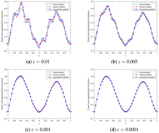
Figure 1. Example 1: $p=2$, $E=9$, $\alpha =0.2,\beta =1.7$, the exact and regularization solutions for various $\epsilon$.

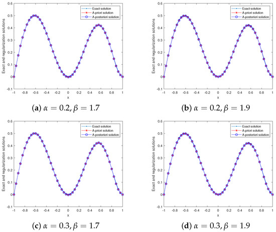
Figure 2. Example 1: $p=2$, $E=9$, $\epsilon =0.0001$, the exact and regularization solutions for various $\alpha$, $\beta$.

Table 1. Example 1: $p=2$, $\epsilon =0.0001$, the computation results for the relative errors by the Galerkin method and the QBV method.

	$\mathit{\alpha }=\mathbf{0.2}\mathit{\beta }=\mathbf{1.7}$	$\mathit{\alpha }=\mathbf{0.2}\mathit{\beta }=\mathbf{1.9}$	$\mathit{\alpha }=\mathbf{0.3}\mathit{\beta }=\mathbf{1.7}$	$\mathit{\alpha }=\mathbf{0.3}\mathit{\beta }=\mathbf{1.9}$
${ϵ}_{pri,Galerkin}\left(u\right)$	0.007435	0.009797	0.007511	0.009825
${ϵ}_{post,Galerkin}\left(u\right)$	0.007348	0.009356	0.007431	0.009825
${ϵ}_{pri,QBV}\left(u\right)$	0.0633	0.0855	0.0688	0.0926
${ϵ}_{post,QBV}\left(u\right)$	0.0216	0.0317	0.0234	0.0341

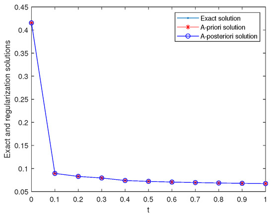
Figure 3. Example 1: $\alpha =0.2,\beta =1.7$, the exact and regularization solutions for various t at $x=0.6$.

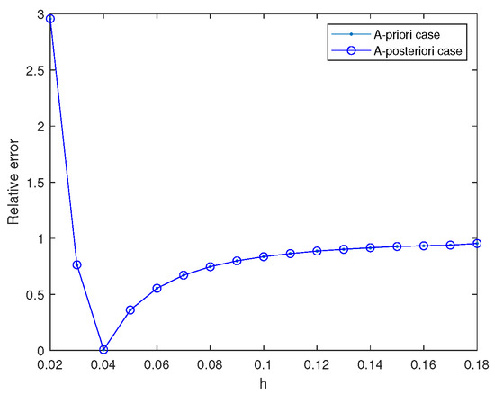
Figure 4. Example 1: $\alpha =0.2,\beta =1.7$, the relative error for various step h.

Example 2. 

In the forward problem (12), we take:

$$\begin{array}{c}\hfill \begin{array}{cc}\hfill & h\left(x\right)=\left\{\begin{array}{c}-4x^2+4,x\in [-1,0],\hfill \\ -4x+4,x\in [0,\frac{1}{2}],\hfill \\ e^{x-\frac{1}{2}}+1,x\in [\frac{1}{2},1].\hfill \end{array}\right.\hfill \\ \hfill & f(x,t)=tsin\left(x\right).\hfill \end{array}\end{array}$$

Note, that $h\left(x\right)$ is a continuous function, but it only belongs to $H^1(\Omega )\subset L^2(\Omega )$, and ${\parallel u(x,0)\parallel }_{H^1}$=${\parallel h\left(x\right)\parallel }_{H^1}\le 7$; thus, we chose a priori bound $E=7$. For $\epsilon =0.0001$, $p=1$, $\alpha =0.2$ and $0.3$, $\beta =1.7$, and $1.9$, the computation results of the exact and regularization solutions are shown in Figure 5. For $p=1$ and $\epsilon =0.0001$, the calculation results for the relative errors by the Galerkin method and the QBV method are presented in Table 2. Figure 5 and Table 2 show that our method is also effective in solving the case in which the solution of the backward problem only belongs to the space $H^1(\Omega )$. Meanwhile, Table 2 also shows that our method is slightly better than the QBV method in dealing with the inverse problem whose solution belongs to the space $H^1(\Omega )$.

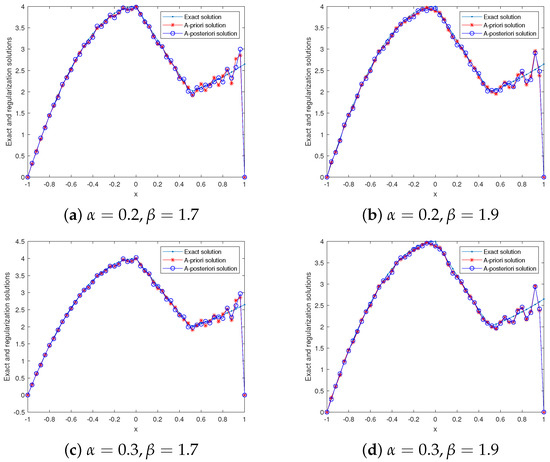
Figure 5. Example 2: $p=1$, $E=7$, $\epsilon =0.0001$, the exact and regularization solutions for various $\alpha$, $\beta$.

Table 2. Example 2: $p=1$, $\epsilon =0.0001$, the computation results for the relative errors by the Galerkin method and the QBV method.

	$\mathit{\alpha }=\mathbf{0.2}\mathit{\beta }=\mathbf{1.7}$	$\mathit{\alpha }=\mathbf{0.2}\mathit{\beta }=\mathbf{1.9}$	$\mathit{\alpha }=\mathbf{0.3}\mathit{\beta }=\mathbf{1.7}$	$\mathit{\alpha }=\mathbf{0.3}\mathit{\beta }=\mathbf{1.9}$
${ϵ}_{pri,Galerkin}\left(u\right)$	0.135513	0.136483	0.135539	0.136502
${ϵ}_{post,Galerkin}\left(u\right)$	0.135468	0.135671	0.135407	0.136065
${ϵ}_{pri,QBV}\left(u\right)$	0.151263	0.165846	0.155099	0.168608
${ϵ}_{post,QBV}\left(u\right)$	0.135912	0.149952	0.136676	0.151806

Example 3. 

In the forward problem (12), $h\left(x\right)\subset L^2(\Omega )$ is taken as a non-smooth function:

$$\begin{array}{c}\hfill \begin{array}{cc}\hfill & h\left(x\right)=\left\{\begin{array}{c}0,x\in [-1,-\frac{1}{2}],\hfill \\ 4,x\in [-\frac{1}{2},0],\hfill \\ -2,x\in [0,\frac{1}{2}],\hfill \\ 0,x\in [\frac{1}{2},1].\hfill \end{array}\right.\hfill \\ \hfill & f(x,t)=tsin\left(x\right).\hfill \end{array}\end{array}$$

Since ${\parallel u(x,0)\parallel }_{L^2}={\parallel h\left(x\right)\parallel }_{L^2}=\sqrt{10}<4$, we took $E=4$, and selected $p=2$ to perform the numerical experiment. For $\epsilon =0.01$, $p=2$, $\alpha =0.2$ and $0.3$, $\beta =1.7$, and $1.9$, the computation results of the exact and regularization solutions are shown in Figure 6. For $E=4$, $p=2$, and $\epsilon =0.01$, the calculation results for the relative errors and a priori and a posteriori regularization parameters are presented in Table 3. Figure 6 and Table 3 show that our method is also effective in solving the inverse problem whose solution is a non-smooth function.

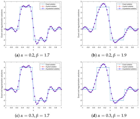
Figure 6. Example 3: $p=2$, $E=4$, $\epsilon =0.01$, the exact and regularization solutions for various $\alpha$, $\beta$.

Table 3. Example 3: $p=2$, $E=4$, $\epsilon =0.01$, the computation results for the relative error and regularization parameter.

	$\mathit{\alpha }=\mathbf{0.2}\mathit{\beta }=\mathbf{1.7}$	$\mathit{\alpha }=\mathbf{0.2}\mathit{\beta }=\mathbf{1.9}$	$\mathit{\alpha }=\mathbf{0.3}\mathit{\beta }=\mathbf{1.7}$	$\mathit{\alpha }=\mathbf{0.3}\mathit{\beta }=\mathbf{1.9}$
$N_{pri}$	12	10	12	10
$N_{post}$	13	11	13	11
${ϵ}_{pri}\left(u\right)$	0.279469	0.344757	0.279498	0.344775
${ϵ}_{post}\left(u\right)$	0.279469	0.344757	0.279498	0.344775

7. Conclusions and Further Discussions

This article studies a backward problem of the time-space fractional parabolic equation. This problem is ill-posed in the sense that its solution is unstable. We prove the existence and uniqueness of a solution and conditional stability for the inverse problem. Based on the ill-posedness analysis, a Galerkin regularization method is constructed to recover the stability of the solution, and a priori and a posteriori convergence results are derived. Additionally, by making some numerical experiments we also verified the simulation effect of our method. Numerical results show that the Galerkin method is stable and feasible in solving the considered problem.

This paper mainly researches the Galerkin regularization theory and numerical algorithm for the case of continuous datum, which satisfy (4), (5). We point out that in this method we also can encounter the case of discrete data, but at this moment we first need solve the discrete system (31) with noisy data ${\gamma }^{\delta }$, and then according to (30) to compute the regularization solution. Meanwhile, a priori and a posteriori convergence results need to be derived. In fact, we have tried and derived a similar a priori convergence result with the case of continuous data. However, for the a posteriori convergence result, at present we have not explored the appropriate selection rule of the regularization parameter. In future works, we will continue to consider and overcome this difficulty.

References

- Magin, E.L. Fractional calculus models of complex dynamics in biological tissues. Comput. Math. Appl. 2009, 59, 1586–1593. [Google Scholar] [CrossRef]
- Sopasakis, P.; Sarimveis, H.; Macheras, P.; Dokoumetzidis, A. Fractional calculus in pharmacokinetics. J. Pharmacokinet. Pharmacodyn. 2018, 45, 107–125. [Google Scholar] [CrossRef] [PubMed]
- Tenreiro Machado, J.A.; Mata, M.E.; Lopes, A.M. Fractional dynamics and pseudo-phase space of country economic processes. Mathematics 2020, 8, 81. [Google Scholar] [CrossRef]
- Ionescu, C.; Lopes, A.; Copot, D.; Machado, J.T.; Bates, J.H. The role of fractional calculus in modeling biological phenomena: A review. Commun. Nonlinear Sci. Numer. Simul. 2017, 51, 141–159. [Google Scholar] [CrossRef]
- Liu, S.S.; Sun, F.Q.; Feng, L.X. Regularization of inverse source problem for fractional diffusion equation with Riemann-Liouville derivative. Comput. Appl. Math. 2021, 40, 112. [Google Scholar] [CrossRef]
- Sun, L.L.; Wei, T. Identification of the zeroth-order coefficient in a time fractional diffusion equation. Appl. Numer. Math. 2017, 111, 160–180. [Google Scholar] [CrossRef]
- Tran, B.N.; Nguyen, H.T.; Mokhtar, K. Regularization of a sideways problem for a time-fractional diffusion equation with nonlinear source. J. Inverse Ill-Posed Probl. 2020, 28, 1–29. [Google Scholar]
- Zhao, J.; Liu, S.; Liu, T. An inverse problem for space-fractional backward diffusion problem. Math. Methods Appl. Sci. 2014, 37, 1147–1158. [Google Scholar] [CrossRef]
- Podlubny, I. Fractional Differential Equations; Academic Press: San Diego, CA, USA, 1999. [Google Scholar]
- Tatar, S.; Tnaztepe, R.; Ulusoy, S. Determination of an unknown source term in a space-time fractional diffusion equation. J. Fract. Calc. Appl. 2015, 6, 83–90. [Google Scholar]
- Dipierro, S.; Lippi, E.P.; Valdinoci, E. (Non) local logistic equations with Neumann conditions. arXiv 2021, arXiv:2101.02315. [Google Scholar] [CrossRef]
- Cassani, D.; Vilasi, L.; Wang, Y.J. Local versus nonlocal elliptic equations:short-long range field interactions. Adv. Nonlinear Anal. 2021, 10, 895–921. [Google Scholar] [CrossRef]
- Liu, J.J.; Yamamoto, M. A backward problem for the time-fractional diffusion equation. Appl. Anal. 2010, 89, 1769–1788. [Google Scholar] [CrossRef]
- Yang, F.; Ren, Y.P.; Li, X.X. The quasi-reversibility method for a final value problem of the time-fractional diffusion equation with inhomogeneous source. Math. Methods Appl. Sci. 2018, 41, 1774–1795. [Google Scholar] [CrossRef]
- Wang, L.Y.; Liu, J.J. Total variation regularization for a backward time-fractional diffusion problem. Inverse Probl. 2013, 29, 1–22. [Google Scholar] [CrossRef]
- Yang, S.P.; Xiong, X.T.; Nie, Y. Iterated fractional Tikhonov regularization method for solving the spherically symmetric backward time-fractional diffusion equation. Appl. Numer. Math. 2021, 160, 217–241. [Google Scholar] [CrossRef]
- Ren, C.; Xu, X.; Lu, S. Regularization by projection for a backward problem of the time-fractional diffusion equation. J. Inverse Ill-Posed Probl. 2014, 22, 121–139. [Google Scholar] [CrossRef]
- Wang, L.Y.; Liu, J.J. Data regularization for a backward time-fractional diffusion problem. Comput. Math. Appl. 2012, 64, 3613–3626. [Google Scholar] [CrossRef]
- Wang, J.G.; Wei, T.; Zhou, Y.B. Optimal error bound and simplified Tikhonov regularization method for a backward problem for the time-fractional diffusion equation. J. Comput. Appl. Math. 2015, 279, 277–292. [Google Scholar] [CrossRef]
- Dinh, L.L.; Kim, V.H.; Duy, B.H.; Reza, S. On backward problem for fractional spherically symmetric diffusion equation with observation data of nonlocal type. Adv. Differ. Equ. 2021, 2021, 445. [Google Scholar]
- Zheng, G.H.; Wei, T. Two regularization methods for solving a Riesz-Feller space-fractional backward diffusion problem. Inverse Probl. 2010, 26, 1–23. [Google Scholar] [CrossRef]
- Cheng, H.; Fu, C.L.; Zheng, G.H.; Gao, J. A regularization for a Riesz-Feller space-fractional backward diffusion problem. Inverse Probl. Sci. Eng. 2014, 22, 860–872. [Google Scholar] [CrossRef]
- Yang, F.; Li, X.X.; Li, D.G.; Wang, L. The simplified Tikhonov regularization method for solving a Riesz-Feller space-fractional backward diffusion problem. Math. Comput. Sci. 2017, 11, 91–110. [Google Scholar] [CrossRef]
- Zheng, G.H.; Zhang, Q.G. Recovering the initial distribution for space-fractional diffusion equation by a logarithmic regularization method. Appl. Math. Lett. 2016, 61, 143–148. [Google Scholar] [CrossRef]
- Zheng, G.H.; Zhang, Q.G. Determining the initial distribution in space-fractional diffusion by a negative exponential regularization method. Inverse Probl. Sci. Eng. 2017, 25, 965–977. [Google Scholar] [CrossRef]
- Zheng, G.H.; Zhang, Q.G. Solving the backward problem for space-fractional diffusion equation by a fractional Tikhonov regularization method. Math. Comput. Simul. 2018, 148, 37–47. [Google Scholar] [CrossRef]
- Zhang, Z.Q.; Wei, T. An optimal regularization method for space-fractional backward diffusion problem. Math. Comput. Simul. 2013, 92, 14–27. [Google Scholar] [CrossRef]
- Liu, S.S.; Feng, L.X. Optimal error bound and modified kernel method for a space-fractional backward diffusion problem. Adv. Differ. Equ. 2018, 2018, 268. [Google Scholar] [CrossRef]
- Zhang, H.W.; Zhang, X.J. Solving the Riesz-Feller space-fractional backward diffusion problem by a generalized Tikhonov method. Adv. Differ. Equ. 2020, 2020, 376–384. [Google Scholar] [CrossRef]
- Dou, F.F.; Hon, Y.C. Fundamental kernel-based method for backward space-time fractional diffusion problem. Comput. Math. Appl. 2016, 71, 356–367. [Google Scholar] [CrossRef]
- Jia, J.X.; Peng, J.G.; Gao, J.H.; Li, Y. Backward problem for a time-space fractional diffusion equation. Inverse Probl. Imaging 2018, 12, 773–799. [Google Scholar] [CrossRef]
- Trong, D.D.; Hai, D.N.D.; Dien, N.M. On a time-space fractional backward diffusion problem with inexact orders. Comput. Math. Appl. 2019, 78, 1572–1593. [Google Scholar] [CrossRef]
- Wang, J.L.; Xiong, X.T.; Cao, X.X. Fractional Tikhonov regularization method for a time-fractional backward heat equation with a fractional Laplacian. J. Partial. Differ. Equ. 2018, 4, 333–342. [Google Scholar]
- Djennadi, S.; Shawagfeh, N.; Abu Arqub, O. A fractional Tikhonov regularization method for an inverse backward and source problems in the time-space fractional diffusion equations. Chaos Solitons Fractals 2021, 150, 111127. [Google Scholar] [CrossRef]
- Yang, F.; Zhang, Y.; Liu, X.; Li, X. The quasi-boundary value method for identifying the initial value of the space-time fractional diffusion equation. Acta Math. Sci. 2020, 40, 641–658. [Google Scholar] [CrossRef]
- Feng, X.L.; Zhao, M.X.; Qian, Z. A Tikhonov regularization method for solving a backward time-space fractional diffusion problem. J. Comput. Appl. Math. 2022, 411, 114236. [Google Scholar] [CrossRef]
- Trong, D.D.; Hai, D.N. Backward problem for time-space fractional diffusion equations in Hilbert scales. Comput. Math. Appl. 2021, 93, 253–264. [Google Scholar] [CrossRef]
- Asadzadeh, M.; Beilina, L. A posteriori error analysis in a globally convergent numerical method for a hyperbolic coefficient inverse. Inverse Probl. 2010, 26, 115–127. [Google Scholar] [CrossRef]
- Yeganeh, S.; Mokhtari, R.; Hesthaven, J.S. Space-dependent source determination in a time-fractional diffusion equation using a local discontinuous Galerkin method. Bit Numer. Math. 2017, 57, 685–707. [Google Scholar] [CrossRef]
- Qasemi, S.; Rostamy, D.; Abdollahi, N. The time-fractional diffusion inverse problem subject to an extra measurement by a local discontinuous Galerkin method. Bit Numer. Math. 2019, 59, 183–212. [Google Scholar] [CrossRef]
- Xiong, X.T.; Zhao, X.; Wang, J. Spectral Galerkin method and its application to a Cauchy problem of Helmholtz equation. Numer. Algorithms 2013, 63, 691–711. [Google Scholar] [CrossRef]
- Kien, B.T.; Qin, X.; Wen, C.F.; Yao, J.C. The Galerkin Method and Regularization for Variational Inequalities in Reflexive Banach Spaces. J. Optim. Theory Appl. 2021, 189, 578–596. [Google Scholar] [CrossRef]
- Zhao, Q.L. Regularization of Three Inverse Boundary Value Problems. Master’s Thesis, Lanzhou University, Lanzhou, China, 2008. (In Chinese). [Google Scholar]
- Kirsch, A. An Introduction to the Mathematical Theory of Inverse Problems; Springer: New York, NY, USA, 2011. [Google Scholar]
- Liu, J.J. Regularization Method for Ill-Posed Problem and Its Application; Science Press: Beijing, China, 2005. (In Chinese) [Google Scholar]
- Kilbas, A.A.; Srivastava, H.M.; Trujillo, J.J. Theory and applications of fractional differential equations. North-Holl. Math. Stud. 2006, 204, 2453–2461. [Google Scholar]
- Sakamoto, K.; Yamamoto, M. Initial value/boundary value problems for fractional diffusion-wave equations and applications to some inverse problems. J. Math. Anal. Appl. 2011, 382, 426–447. [Google Scholar] [CrossRef]
- Pollard, H. The completely monotonic character of the Mittag–Leffler function Eα(−x). Bull. Am. Math. Soc. 1948, 54, 1115–1116. [Google Scholar] [CrossRef]
- Mishura, Y.S. Stochastic Calculus for Fractional Brownian Motion and Related Processes; Springer: Berlin, Germany, 2008. [Google Scholar]
- Morozov, V.A.; Nashed, Z.; Aries, A.B. Methods for Solving Incorrectly Posed Problems; Springer: New York, NY, USA, 1984. [Google Scholar]
- Podlubny, I.; Kaccenak, M. Mittag–Leffler Function. The Matlabroutine. 2006. Available online: http://www.mathworks.com/matlabcentral/fileexchange (accessed on 26 February 2023).
Disclaimer/Publisher’s Note: The statements, opinions and data contained in all publications are solely those of the individual author(s) and contributor(s) and not of MDPI and/or the editor(s). MDPI and/or the editor(s) disclaim responsibility for any injury to people or property resulting from any ideas, methods, instructions or products referred to in the content. |
© 2023 by the authors. Licensee MDPI, Basel, Switzerland. This article is an open access article distributed under the terms and conditions of the Creative Commons Attribution (CC BY) license (https://creativecommons.org/licenses/by/4.0/).