A Comparative Study of the Fractional Partial Differential Equations via Novel Transform

Abstract

In comparison to fractional-order differential equations, integer-order differential equations generally fail to properly explain a variety of phenomena in numerous branches of science and engineering. This article implements efficient analytical techniques within the Caputo operator to investigate the solutions of some fractional partial differential equations. The Adomian decomposition method, homotopy perturbation method, and Elzaki transformation are used to calculate the results for the specified issues. In the current procedures, we first used the Elzaki transform to simplify the problems and then applied the decomposition and perturbation methods to obtain comprehensive results for the problems. For each targeted problem, the generalized schemes of the suggested methods are derived under the influence of each fractional derivative operator. The current approaches give a series-form solution with easily computable components and a higher rate of convergence to the precise solution of the targeted problems. It is observed that the derived solutions have a strong connection to the actual solutions of each problem as the number of terms in the series solution of the problems increases. Graphs in two and three dimensions are used to plot the solution of the proposed fractional models. The methods used currently are simple and efficient for dealing with fractional-order problems. The primary benefit of the suggested methods is less computational time. The results of the current study will be regarded as a helpful tool for dealing with the solution of fractional partial differential equations.

1. Introduction

Fractional calculus has been the subject of extensive investigation for a long time. In the subject of fractional calculus, new methods and mechanisms are constantly being developed which enable the discovery of significant, difficult insights and previously unknown connections across many fields of physics. The calculus theory was developed in the seventeenth century by Newton and Leibniz. Leibniz developed the integral and derivative notations that are still in use these days. Later, any real order was added to the definition of the terms’ derivatives and integrals. Lacroix introduced the idea of a noninteger-order derivative for the first time in 1819. Abel examined the initial application in 1823 [1]. Therefore, the aforementioned field received considerable attention from Fourier, Liouville, Riemann, Grunwald, Letnikov, etc. [2,3]. Fractional order differentiation and integration do not have specific definitions, whereas arbitrary order differentiation and integration offer an expansion of the classical order. The definitions of arbitrary-order derivatives and integrations have been introduced by many academics in different ways. The definitions of Caputo and Riemann–Liouvilli among all these are the most broadly applicable. All of these approaches are only expansions of the techniques already used to address the integer case models because the noninteger derivative simplifies the integer derivative to any order [4,5]. Thus, the memory effect is a term that is widely used to describe the study of the dynamics of the function fractionally. The classical derivatives are gradually shown using the nonlocality of the fractional operators. Fractional operators are used to define complex memories and a range of other objects that can be studied using standard mathematical methods like classical differential calculus. Although the application of the FC concept across several academic areas is still in the early stages, FC is currently a very promising tool due to its broadening use in the dynamics of complex nonlinear occurrences.

The main reason for studying numerical methods for fractional differential equations (FDEs) is that fractional derivative models are becoming more and better liked by the entire scientific community. Nonlinear partial differential equations (PDEs) have been a popular subject in the field of nonlinear science and have been used to describe problems in a variety of areas, including ecology and economic systems, image processing, quantum physics, and epidemiology. PDEs are frequently utilized in a variety of physical applications, such as supersonic and turbulent flow, magnetohydrodynamic movement through pipes, wave dispersion and propagation, computational fluid dynamics, magnetic resonance imaging, population modeling, medical imaging, electrically signaling nerves, and others [6,7,8]. To learn more, consider the reference mentioned in [9]. The widespread nature of PDE has been confirmed by a fairly precise evaluation of the number of COVID patients [10,11]. PDE can be used to predict the shape of COVID-19, as seen in [12]. However, for several difficult problems in these domains, the fractional PDE is more precise than the integer-order partial differential equation. Therefore, establishing numerical solutions for fractional PDEs is important.

The solution of PDEs can be made simpler by using symmetry, which is a fundamental idea in both mathematics and physics. Particularly, applying symmetry to fractional PDE solutions can substantially simplify mathematical analysis and provide accurate or approximative solutions [13,14]. In a fractional PDE, symmetry can be employed to limit the number of independent variables, which will make the solution process easier. In addition, solutions that are invariant under specific transformations like translations, rotations, and scaling can be found using symmetry. This may result in conclusions that are simpler to understand and have greater physical significance. In general, symmetry is an effective tool for solving fractional PDEs and can be very helpful in explaining the underlying physical phenomena [15,16]. A summary of FDEs and their applications may be found in various significant references. In [17,18], a full review of fractional calculus, FDEs, and their applications in a variety of domains is covered. In the study of viscoelasticity, the theory of FDEs and its applications have been examined [19,20].

Due to the complexity of fractional orders, it is difficult to find analytical solutions for the majority of FDEs. As a result, numerical solutions are found for the aforementioned FDEs. For this purpose, various numerical algorithms have been developed [21,22]. Spectral methods are numerical methods that use spectral representations of the solution to approximate the solution of a differential equation. The tau, collocation, and Galerkin methods are examples of spectral methods that have been used for solving FDEs. The tau method is a spectral method that uses a shifted Legendre polynomial basis to approximate the solution of FDEs. This collocation method is a spectral method that uses a basis of orthogonal polynomials to approximate the solution of FDEs at collocation points. Several studies have demonstrated the effectiveness of spectral methods for solving FDEs [23,24,25,26,27,28]. Overall, spectral methods such as the tau, collocation, and Galerkin methods have proven to be effective for solving FDEs and time-fractional differential equations. These methods provide accurate solutions with high efficiency, making them valuable tools for modeling and simulation in various fields.

It is becoming clear that fractional partial differential equations (FPDEs) are an effective modeling tool for complex multiscale occurrences, including those involving overlapping microscopic and macroscopic dimensions. The fractional order of the derivatives in FPDEs can be a function of space and time or even a distribution, in contrast to integer-order PDEs. It develops outstanding possibilities for modeling and simulating multi-physics phenomena, such as the seamless transition from wave propagation to diffusion or from local to nonlocal dynamics. Numerous well-known scholars have made contributions to this area due to the importance of analytically solving FPDEs in engineering and science. Several methods have been investigated in order to investigate approximate solutions to FPDEs, including the Yang transform decomposition method for fractional-order diffusion equations [29] and time-fractional phi-four equations [30], the reduced differential transform method for coupled time fractional nonlinear evolution equations [31], and the natural transform decomposition method for the solution of fractional Caudrey–Dodd–Gibbon equations [32] and fractional Kuramoto–Sivashinsky equations [33], fractional homotopy analysis method for solving the fractional epidemic model [34] and fractional KdV–Burgers–Kuramoto equation [35], homotopy perturbation transform method for solving fractional Noyes-Field model [36] and time-fractional Fisher’s equation [37], variational iteration transform method for fractional-order Newell–Whitehead–Segel equations [38] and for fractional-order Boussinesq equation [39], approximate analytical method for the solution of time-fractional telegraph equations [40] and the Adams–Bashforth method to study the time-fractional Tricomi equation with nonlocal and nonsingular kernel [41] and many more [42,43,44,45,46,47,48,49].

This study described two novel approaches: the Elzaki transform decomposition method (ETDM) and the homotopy perturbation transform method (HPTM). The Elzaki transform was introduced by Tarig Elzaki to make solving ordinary and partial differential equations in the time domain much easier. Since the 1980s, Adomian has developed a numerical approach for solving functional equations [50,51]. It gives analysis in the form of a series that converges quickly towards the exact solutions. It is considered a powerful method for solving both linear and nonlinear, homogeneous and nonhomogeneous partial and differential equations of integer and noninteger order. The homotopy perturbation method (HPM), which he first suggested in 1998 [52] and later advanced and enhanced [53,54], leads to a very fast convergence solution in the form of a series. To summarize, the Elzaki transform approach is initially utilized to approximate the Caputo-type temporal fractional derivative and turn the initial FPDE into its equivalent PDE. The resultant PDE is then solved using the adomian decomposition method and the homotopy perturbation approach, leading to quick and low-cost methods for solving the original FPDE. Typically, only one iteration yields high precision in the solution, making it an effective and valuable mathematical tool for nonlinear equations.

The following is how this study is presented: In Section 2, fractional derivative definitions and the history of the natural transform method are given. Section 3 and Section 4 address the application model of FDEs employing the provided techniques. Section 5 gives a convergence analysis of the suggested approaches. In Section 6, we solve fractional FDEs. Our final conclusions are in Section 7.

2. Preliminaries

Here we recall some basic definitions concerned with fractional calculus.

Definition 1. 

The Riemann–Liouville’s arbitrary order operator is defined by [55,56,57]

$$D^{\sigma }\mathcal{K}\left(\rho \right)=\left\{\begin{array}{c}\frac{d^{\varsigma }}{d{\rho }^{\varsigma }}\mathcal{K}\left(\rho \right),\sigma =\varsigma ,\hfill \\ \frac{1}{\mathsf{\Gamma }(\varsigma -\sigma )}\frac{d}{d{\rho }^{\varsigma }}{\int }_0^{\rho }\frac{\mathcal{K}\left(\rho \right)}{{(\rho -\psi )}^{\sigma -\varsigma +1}}d\psi ,\varsigma -1<\sigma <\varsigma ,\hfill \end{array}\right.$$

where $\varsigma \in Z^{+}$, $\sigma \in R^{+}$ and

$$D^{-\sigma }\mathcal{K}\left(\rho \right)=\frac{1}{\mathsf{\Gamma }\left(\sigma \right)}{\int }_0^{\rho }{(\rho -\psi )}^{\sigma -1}\mathcal{K}\left(\psi \right)d\psi ,0<\sigma \le 1.$$

Definition 2. 

The Riemann–Liouville’s arbitrary order integral operator is defined by [55,56,57]

$$J^{\sigma }\mathcal{K}\left(\rho \right)=\frac{1}{\mathsf{\Gamma }\left(\sigma \right)}{\int }_0^{\rho }{(\rho -\psi )}^{\sigma -1}\mathcal{K}\left(\rho \right)d\rho ,\rho >0,\sigma >0.$$

with the following properties

$$\begin{array}{c}\hfill J^{\sigma }{\rho }^{\varsigma }=\frac{\mathsf{\Gamma }(\varsigma +1)}{\mathsf{\Gamma }(\varsigma +\sigma +1)}{\rho }^{\varsigma +\psi },\\ \hfill D^{\sigma }{\rho }^{\varsigma }=\frac{\mathsf{\Gamma }(\varsigma +1)}{\mathsf{\Gamma }(\varsigma -\sigma +1)}{\rho }^{\varsigma -\psi },\end{array}$$

Definition 3. 

The Caputo’s arbitrary order derivative is defined by [55,56,57]

$$D^{\sigma }\mathcal{K}\left(\rho \right)=\left\{\begin{array}{c}\frac{1}{\mathsf{\Gamma }(\varsigma -\sigma )}{\int }_0^{\rho }\frac{{\mathcal{K}}^{\varsigma }\left(\psi \right)}{{(\rho -\psi )}^{\sigma -\varsigma +1}}d\psi ,\varsigma -1<\sigma <\varsigma ,\hfill \\ \frac{d^{\varsigma }}{d{\rho }^{\varsigma }}\mathcal{K}\left(\rho \right),\varsigma =\sigma .\hfill \end{array}\right.$$

(1)

having the following properties

$$\begin{array}{cc}\hfill J_{\rho }^{\sigma }{D}_{\rho }^{\sigma }\mathcal{K}\left(\rho \right)& =g\left(\rho \right)-{\displaystyle \sum _{k=0}^m}{g}^k\left(0^{+}\right)\frac{{\rho }^k}{k!},for\rho >0,and\varsigma -1<\sigma \le \varsigma ,\varsigma \in N.\hfill \\ \hfill D_{\rho }^{\sigma }{J}_{\rho }^{\sigma }\mathcal{K}\left(\rho \right)& =g\left(\rho \right).\hfill \end{array}$$

(2)

Definition 4. 

The Elzaki transform (ET) of the function $\mathcal{K}\left(\zeta \right)$ is taken as [58]

$$\mathtt{E}\left\{\mathcal{K}\left(\zeta \right)\right\}=M\left(u\right)=u{\int }_u^{\infty }{e}^{\frac{-\zeta }{u}}\mathcal{K}\left(\zeta \right)d\zeta ,\zeta >0.$$

(3)

Definition 5. 

The ET of fractional Caputo operator is defined by [59]

$$\mathtt{E}\left[D_{\rho }^{\sigma }\mathcal{K}\left(\rho \right)\right]=u^{-\sigma }\mathtt{E}\left[\mathcal{K}\left(\rho \right)\right]-\sum _{i=0}^{n-1}{u}^{2-\sigma +i}{\mathcal{K}}^{\left(i\right)}\left(0\right),wheren-1<\sigma <n.$$

The transformation of Elzaki is a very useful and powerful method for solving the integral equation that cannot be solved by the Sumudu transformation method.

In order to obtain ET of partial derivatives, integration by parts may be used in Equation (2) as given.

• ${\displaystyle \mathtt{E}\left[{\zeta }^n\right]=n!u^{n+2}.}$
• ${\displaystyle \mathtt{E}\left[{\mathcal{K}}^{\prime }\right]=\frac{M\left(u\right)}{u}-u\mathcal{K}\left(0\right).}$
• ${\displaystyle \mathtt{E}\left[{\mathcal{K}}^{″}\right]=\frac{M\left(u\right)}{u^2}-\mathcal{K}\left(0\right)-u{\mathcal{K}}^{\prime }\left(0\right).}$
• ${\displaystyle \mathtt{E}\left[{\mathcal{K}}^n\right]=\frac{M\left(u\right)}{u^2}-\sum _{i=0}^{n-1}{u}^{2-n+i}{\mathcal{K}}^{\left(i\right)}\left(0\right).}$

3. Formulation of HPTM

In this part, we construct the general methodology of HPTM for solving the FPDEs:

$$D_{\zeta }^{\sigma }\mathcal{K}(\rho ,\zeta )=[{\mathcal{F}}_1+{\mathcal{G}}_1]\mathcal{K}(\rho ,\zeta ),\rho ,\zeta >00<\sigma \le 1,$$

(4)

having the initial condition

$$\mathcal{K}(\rho ,0)=\vartheta \left(\rho \right).$$

with $D_{\zeta }^{\sigma }=\frac{{\partial }^{\sigma }}{\partial {\zeta }^{\sigma }}$ representing the Caputo derivative of order $\sigma$, and ${\mathcal{F}}_1(\rho ,\zeta ),$ ${\mathcal{F}}_1(\rho ,\zeta )$ are linear and nonlinear operators.

By utilizing Definition 5 when n = 1, we obtain

$$\frac{1}{u^{\sigma }}\{M\left(u\right)-u^2\mathcal{K}(\rho ,0)\}=\mathtt{E}\left[[{\mathcal{F}}_1+{\mathcal{G}}_1]\mathcal{K}(\rho ,\zeta )\right],$$

(5)

then, we obtain

$$M\left(u\right)=u^2\mathcal{K}(\rho ,0)+u^{\sigma }\mathtt{E}\left[[{\mathcal{F}}_1+{\mathcal{G}}_1]\mathcal{K}(\rho ,\zeta )\right],$$

(6)

where M(u) = $\mathtt{E}\left[\mathcal{K}\right(\rho ,\zeta \left)\right]$.

By using inverse ET, we have

$$\mathcal{K}(\rho ,\zeta )=\mathcal{K}(\rho ,0)+{\mathtt{E}}^{-1}\left[u^{\sigma }\mathtt{E}\left[[{\mathcal{F}}_1+{\mathcal{G}}_1]\mathcal{K}(\rho ,\zeta )\right]\right].$$

(7)

Thus by using HPM, we obtain

$$\mathcal{K}(\rho ,\zeta )=\sum _{m=0}^{\infty }{ϵ}^m{\mathcal{K}}_m(\rho ,\zeta ).$$

(8)

where $ϵ\in [0,1]$ is homotopy parameter and the ${\mathcal{K}}_i(\rho ,\zeta ),i=0,1,2,\cdots$ are function yet to be determined.

The nonlinear term is taken as

$${\mathcal{G}}_1\left[\mathcal{K}(\rho ,\zeta )\right]=\sum _{n=0}^{\infty }{ϵ}^n{H}_n(\rho ,\zeta ),$$

(9)

in terms of homotopy polynomial and is calculated as

$$H_n(\rho ,\zeta )=\frac{1}{\mathsf{\Gamma }(n+1)}{D}_{ϵ}^k{\left[{\mathcal{G}}_1\left(\sum _{n=0}^{\infty }{ϵ}^n{\mathcal{K}}_n\right)\right]}_{ϵ=0},$$

(10)

with $D_{ϵ}^n=\frac{{\partial }^n}{\partial {ϵ}^n}.$

By putting (8) and (9) in (7), we have

$$\sum _{n=0}^{\infty }{ϵ}^n{\mathcal{K}}_n(\rho ,\zeta )=\mathcal{K}(\rho ,0)+ϵ\times \left({\mathtt{E}}^{-1}\left[u^{\sigma }\mathtt{E}\{{\mathcal{F}}_1\sum _{n=0}^{\infty }{ϵ}^n{\mathcal{K}}_n(\rho ,\zeta )+\sum _{n=0}^{\infty }{ϵ}^n{H}_n(\rho ,\zeta )\}\right]\right).$$

(11)

By equating the $ϵ$ coefficient with both sides

$$\begin{array}{cc}\hfill & {ϵ}^0:{\mathcal{K}}_0(\rho ,\zeta )=\mathcal{K}(\rho ,0),\hfill \\ \hfill & {ϵ}^1:{\mathcal{K}}_1(\rho ,\zeta )={\mathtt{E}}^{-1}\left[u^{\sigma }\mathtt{E}({\mathcal{F}}_1\left({\mathcal{K}}_0(\rho ,\zeta )\right)+H_0(\rho ,\zeta ))\right],\hfill \\ \hfill & {ϵ}^2:{\mathcal{K}}_2(\rho ,\zeta )={\mathtt{E}}^{-1}\left[u^{\sigma }\mathtt{E}({\mathcal{F}}_1\left({\mathcal{K}}_1(\rho ,\zeta )\right)+H_1(\rho ,\zeta ))\right],\hfill \\ \hfill & ⋮\hfill \\ \hfill & {ϵ}^n:{\mathcal{K}}_n(\rho ,\zeta )={\mathtt{E}}^{-1}\left[u^{\sigma }\mathtt{E}({\mathcal{F}}_1\left({\mathcal{K}}_{n-1}(\rho ,\zeta )\right)+H_{n-1}(\rho ,\zeta ))\right],n>0,n\in N.\hfill \end{array}$$

(12)

Finally, our analytical solution behaves in terms of series as

$$\mathcal{K}(\rho ,\zeta )=\underset{M\to \infty }{lim}\sum _{n=1}^M{\mathcal{K}}_n(\rho ,\zeta ).$$

(13)

4. Formulation of ETDM

In this part, we construct the general methodology of ETDM for solving the FPDEs:

$$D_{\zeta }^{\sigma }\mathcal{K}(\rho ,\zeta )=[{\mathcal{F}}_1+{\mathcal{G}}_1]\mathcal{K}(\rho ,\zeta ),\rho ,\zeta >00<\sigma \le 1,$$

(14)

having the initial condition

$$\mathcal{K}(\rho ,0)=\vartheta \left(\rho \right).$$

with $D_{\zeta }^{\sigma }=\frac{{\partial }^{\sigma }}{\partial {\zeta }^{\sigma }}$ representing the Caputo derivative of order $\sigma$, and ${\mathcal{F}}_1$, ${\mathcal{G}}_1$ are linear and nonlinear operators.

By utilizing the Definition 5 when n = 1, we obtain

$$\begin{array}{cc}\hfill & \frac{1}{u^{\sigma }}\{M\left(u\right)-u^2\mathcal{K}(\rho ,0)\}=\mathtt{E}\left[[{\mathcal{F}}_1+{\mathcal{G}}_1]\mathcal{K}(\rho ,\zeta )\right],\hfill \end{array}$$

(15)

then, we obtain

$$M\left(u\right)=u\mathcal{K}(\rho ,0)+u^{\sigma }\mathtt{E}\left[[{\mathcal{F}}_1+{\mathcal{G}}_1]\mathcal{K}(\rho ,\zeta )\right],$$

(16)

where M(u) = $\mathtt{E}\left[\mathcal{K}\right(\rho ,\zeta \left)\right]$.

By using inverse ET, we have

$$\mathcal{K}(\rho ,\zeta )=\mathcal{K}(\rho ,0)+{\mathtt{E}}^{-1}[u^{\sigma }\mathtt{E}\left[[{\mathcal{F}}_1+{\mathcal{G}}_1]\mathcal{K}(\rho ,\zeta )\right].$$

(17)

Thus, the series form solution is as

$$\mathcal{K}(\rho ,\zeta )=\sum _{n=0}^{\infty }{\mathcal{K}}_n(\rho ,\zeta ).$$

(18)

The illustration of a nonlinear term is as

$${\mathcal{G}}_1\left[\mathcal{K}(\rho ,\zeta )\right]=\sum _{n=0}^{\infty }{\mathcal{A}}_n(\rho ,\zeta ).$$

(19)

with

$${\mathcal{A}}_n(\rho ,\zeta )=\frac{1}{n!}{\left[\frac{{\partial }^n}{\partial {\ell }^n}\left\{{\mathcal{G}}_1\left(\sum _{n=0}^{\infty }{\ell }^n{\mathcal{K}}_n\right)\right\}\right]}_{\ell =0},n=0,1,2,\cdots$$

(20)

By putting (18) and (19) in (17), we obtain

$$\sum _{n=0}^{\infty }{\mathcal{K}}_n(\rho ,\zeta )=\mathcal{K}(\rho ,0)+{\mathtt{E}}^{-1}{u}^{\sigma }\left[\mathtt{E}\left\{{\mathcal{F}}_1\left(\sum _{n=0}^{\infty }{\mathcal{K}}_n(\rho ,\zeta )\right)+\sum _{n=0}^{\infty }{\mathcal{A}}_n(\rho ,\zeta )\right\}\right].$$

(21)

By equating both sides

$${\mathcal{K}}_0(\rho ,\zeta )=\mathcal{K}(\rho ,0),$$

(22)

$${\mathcal{K}}_1(\rho ,\zeta )={\mathtt{E}}^{-1}\left[u^{\sigma }\mathtt{E}\{{\mathcal{F}}_1\left({\mathcal{K}}_0(\rho ,\zeta )\right)+{\mathcal{A}}_0(\rho ,\zeta )\}\right].$$

Finally, our general solution for $m\ge 1$ is illustrated as

$${\mathcal{K}}_{m+1}(\rho ,\zeta )={\mathtt{E}}^{-1}\left[u^{\sigma }\mathtt{E}\{{\mathcal{F}}_1\left({\mathcal{K}}_m(\rho ,\zeta )\right)+{\mathcal{A}}_m(\rho ,\zeta )\}\right].$$

5. Convergence Analysis

In this part, the suggested techniques for convergence analysis are discussed.

Theorem 1. 

Suppose the exact solution of (4) is $G(\rho ,\zeta )$ and let $G(\rho ,\zeta )$, $G_n(\rho ,\zeta )\in H$ and $\alpha \in (0,1)$, where H represents the Hilbert space. The solution obtained ${\sum }_{q=0}^{\infty }{G}_q(\rho ,\zeta )$ will converge $G(\rho ,\zeta )$ if $G_q(\rho ,\zeta )\le G_{q-1}(\rho ,\zeta )\forall q>A$, i.e., for any $\omega >0\exists A>0$, such that $\left|\right|G_{q+n}(\rho ,\zeta )\left|\right|\le \beta ,\forall m,n\in N.$

Proof. 

We take a sequence of ${\sum }_{q=0}^{\infty }{G}_q(\rho ,\zeta ).$

$$\begin{array}{cc}\hfill C_0(\rho ,\zeta )=& G_0(\rho ,\zeta ),\hfill \\ \hfill C_1(\rho ,\zeta )=& G_0(\rho ,\zeta )+G_1(\rho ,\zeta ),\hfill \\ \hfill C_2(\rho ,\zeta )=& G_0(\rho ,\zeta )+G_1(\rho ,\zeta )+G_2(\rho ,\zeta ),\hfill \\ \hfill C_3(\rho ,\zeta )=& G_0(\rho ,\zeta )+G_1(\rho ,\zeta )+G_2(\rho ,\zeta )+G_3(\rho ,\zeta ),\hfill \\ \hfill & ⋮\hfill \\ \hfill C_q(\rho ,\zeta )=& G_0(\rho ,\zeta )+G_1(\rho ,\zeta )+G_2(\rho ,\zeta )+\cdots +G_q(\rho ,\zeta ).\hfill \end{array}$$

(23)

We must demonstrate that $C_q(\rho ,\zeta )$ forms a “Cauchy sequence” in order to achieve the desired outcome. Additionally, let us take

$$\begin{array}{cc}\hfill \left|\right|C_{q+1}(\rho ,\zeta )-C_q(\rho ,\zeta )\left|\right|& =\left|\right|G_{q+1}(\rho ,\zeta )\left|\right|\le \alpha \left|\right|G_q(\rho ,\zeta )\left|\right|\le {\alpha }^2\left|\right|G_{q-1}(\rho ,\zeta )\left|\right|\le {\alpha }^3\left|\right|G_{q-2}(\rho ,\zeta )\left|\right|\cdots \hfill \\ \hfill & \le {\alpha }_{q+1}\left|\right|G_0(\rho ,\zeta )\left|\right|.\hfill \end{array}$$

(24)

For $q,n\in N$, we have

$$\begin{array}{cc}\hfill \left|\right|C_q(\rho ,\zeta )-C_n(\rho ,\zeta )\left|\right|=& \left|\right|G_{q+n}(\rho ,\zeta )\left|\right|=\left|\right|C_q(\rho ,\zeta )-C_{q-1}(\rho ,\zeta )+(C_{q-1}(\rho ,\zeta )-C_{q-2}(\rho ,\zeta ))\hfill \\ \hfill & +(C_{q-2}(\rho ,\zeta )-C_{q-3}(\rho ,\zeta ))+\cdots +(C_{n+1}(\rho ,\zeta )-C_n(\rho ,\zeta ))\left|\right|\hfill \\ \hfill \le & \left|\right|C_q(\rho ,\zeta )-C_{q-1}(\rho ,\zeta )\left|\right|+\left|\right|(C_{q-1}(\rho ,\zeta )-C_{q-2}(\rho ,\zeta ))\left|\right|\hfill \\ \hfill & +\left|\right|(C_{q-2}(\rho ,\zeta )-C_{q-3}(\rho ,\zeta ))\left|\right|+\cdots +\left|\right|(C_{n+1}(\rho ,\zeta )-C_n(\rho ,\zeta ))\left|\right|\hfill \\ \hfill \le & {\alpha }^q\left|\right|G_0(\rho ,\zeta )\left|\right|+{\alpha }^{q-1}\left|\right|G_0(\rho ,\zeta )\left|\right|+\cdots +{\alpha }^{q+1}\left|\right|G_0(\rho ,\zeta )\left|\right|\hfill \\ \hfill =& \left|\right|G_0(\rho ,\zeta )\left|\right|({\alpha }^q+{\alpha }^{q-1}+{\alpha }^{q+1})\hfill \\ \hfill =& \left|\right|G_0(\rho ,\zeta )\left|\right|\frac{1-{\alpha }^{q-n}}{1-{\alpha }^{q+1}}{\alpha }^{n+1}.\hfill \end{array}$$

(25)

As $0<\alpha <1$, and $G_0(\rho ,\zeta )$ are bound, so take $\beta =1-\alpha /(1-{\alpha }_{q-n}){\alpha }^{n+1}\left|\right|G_0(\rho ,\zeta )\left|\right|$, and we obtain

$$\left|\right|G_{q+n}(\rho ,\zeta )\left|\right|\le \beta ,\forall q,n\in N.$$

(26)

Hence, ${\left\{G_q(\rho ,\zeta )\right\}}_{q=0}^{\infty }$ makes a “Cauchy sequence” in H. It proves that the sequence ${\left\{G_q(\rho ,\zeta )\right\}}_{q=0}^{\infty }$ is a convergent sequence with the limit ${lim}_{q\to \infty }{G}_q(\rho ,\zeta )=G(\rho ,\zeta )$ for $\exists G(\rho ,\zeta )\in \mathcal{H}$ which complete the proof. □

Theorem 2. 

Let us assume that ${\sum }_{h=0}^k{G}_h(\rho ,\zeta )$ is finite and $G(\rho ,\zeta )$ reflect the series solution that was found. Assuming $\alpha >0$ such that $\left|\right|G_{h+1}(\rho ,\zeta )\left|\right|\le \left|\right|G_h(\rho ,\zeta )\left|\right|$, the maximum absolute error is given by the following relation.

$$\left|\right|G(\rho ,\zeta )-\sum _{h=0}^k{G}_h(\rho ,\zeta )\left|\right|<\frac{{\alpha }^{k+1}}{1-\alpha }\left|\right|G_0(\rho ,\zeta )\left|\right|.$$

(27)

Proof. 

Suppose ${\sum }_{h=0}^k{G}_h(\rho ,\zeta )$ is finite which implies that ${\sum }_{h=0}^k{G}_h(\rho ,\zeta )<\infty$.

Let us consider

$$\begin{array}{cc}\hfill \left|\right|G(\rho ,\zeta )-{\displaystyle \sum _{h=0}^k}{G}_h(\rho ,\zeta )\left|\right|=& \left|\right|{\displaystyle \sum _{h=k+1}^{\infty }}{G}_h(\rho ,\zeta )\left|\right|\hfill \\ \hfill \le & {\displaystyle \sum _{h=k+1}^{\infty }}\left|\right|G_h(\rho ,\zeta )\left|\right|\hfill \\ \hfill \le & {\displaystyle \sum _{h=k+1}^{\infty }}{\alpha }^h\left|\right|G_0(\rho ,\zeta )\left|\right|\hfill \\ \hfill \le & {\alpha }^{k+1}(1+\alpha +{\alpha }^2+\cdots )\left|\right|G_0(\rho ,\zeta )\left|\right|\hfill \\ \hfill \le & \frac{{\alpha }^{k+1}}{1-\alpha }\left|\right|G_0(\rho ,\zeta )\left|\right|.\hfill \end{array}$$

(28)

which completes the proof of the theorem. □

Theorem 3. 

The result of (14) is unique when $0<({\phi }_1+{\phi }_2)(\frac{{\zeta }^{\sigma }}{\mathsf{\Gamma }(\sigma +1)})<1.$

Proof. 

Let $H=\left(C\right[J],||.|\left|\right)$ with the norm $\left|\right|\varphi \left(\zeta \right)\left|\right|={max}_{\zeta \in J}\left|\varphi \left(\zeta \right)\right|$ is Banach space, ∀ continuous function on $J.$ Let $I:H\to H$ is a nonlinear mapping, where

$${\mathcal{K}}_{l+1}^C={\mathcal{K}}_0^C+{\mathtt{E}}^{-1}\left[u^{\sigma }\mathtt{E}[{\mathcal{F}}_1\left({\mathcal{K}}_l(\rho ,\zeta )\right)+{\mathcal{G}}_1\left({\mathcal{K}}_l(\rho ,\zeta )\right)]\right],l\ge 0.$$

Suppose that $|{\mathcal{F}}_1\left(\mathcal{K}\right)-{\mathcal{F}}_1\left({\mathcal{K}}^{*}\right)|<{\phi }_1|\mathcal{K}-{\mathcal{K}}^{*}|$ and $|{\mathcal{G}}_1\left(\mathcal{K}\right)-{\mathcal{G}}_1\left({\mathcal{K}}^{*}\right)|<{\phi }_2|\mathcal{K}-{\mathcal{K}}^{*}|$, where $\mathcal{K}:=\mathcal{K}(\rho ,\zeta )$ and ${\mathcal{K}}^{*}:={\mathcal{K}}^{*}(\rho ,\zeta )$ are are two different function values and ${\phi }_1$,${\phi }_2$ are Lipschitz constants.

$$\begin{array}{cc}\hfill \left|\right|I\mathcal{K}-I{\mathcal{K}}^{*}\left|\right|& \le ma{x}_{t\in J}|{\mathtt{E}}^{-1}[u^{\sigma }\mathtt{E}[{\mathcal{F}}_1\left(\mathcal{K}\right)-{\mathcal{F}}_1\left({\mathcal{K}}^{*}\right)]\hfill \\ \hfill & +u^{\sigma }\mathtt{E}[{\mathcal{G}}_1\left(\mathcal{K}\right)-{\mathcal{G}}_1\left({\mathcal{K}}^{*}\right)]\left|\right]\hfill \\ \hfill & \le ma{x}_{\zeta \in J}[{\phi }_1{\mathtt{E}}^{-1}[u^{\sigma }\mathtt{E}\left[\right|\mathcal{K}-{\mathcal{K}}^{*}\left|\right]]\hfill \\ \hfill & +{\phi }_2{\mathtt{E}}^{-1}[u^{\sigma }\mathtt{E}\left[\right|\mathcal{K}-{\mathcal{K}}^{*}\left|\right]\left]\right]\hfill \\ \hfill & \le ma{x}_{t\in J}({\phi }_1+{\phi }_2)\left[{\mathtt{E}}^{-1}[u^{\sigma }\mathtt{E}|\mathcal{K}-{\mathcal{K}}^{*}\left|\right]\right]\hfill \\ \hfill & \le ({\phi }_1+{\phi }_2)\left[{\mathtt{E}}^{-1}[u^{\sigma }\mathtt{E}\left|\right|\mathcal{K}-{\mathcal{K}}^{*}\left|\right|]\right]\hfill \\ \hfill & =({\phi }_1+{\phi }_2)\left(\frac{{\zeta }^{\sigma }}{\mathsf{\Gamma }(\sigma +1)}\right)\left|\right|\mathcal{K}-{\mathcal{K}}^{*}\left|\right|\hfill \end{array}$$

(29)

I is a contraction as $0<({\phi }_1+{\phi }_2)(\frac{{\zeta }^{\sigma }}{\mathsf{\Gamma }(\sigma +1)})<1$. From the Banach fixed-point theorem the result of (14) is unique. □

Theorem 4. 

The result of (14) is convergent.

Proof. 

Let ${\mathcal{K}}_m={\sum }_{r=0}^m{\mathcal{K}}_r(\rho ,\zeta )$. To show that ${\mathcal{K}}_m$ is a Cauchy sequence in H. Let

$$\begin{array}{cc}\hfill \left|\right|{\mathcal{K}}_m-{\mathcal{K}}_n\left|\right|& =ma{x}_{\zeta \in J}|{\displaystyle \sum _{r=n+1}^m}{\mathcal{K}}_r|,n=1,2,3,\cdots \hfill \\ \hfill & \le ma{x}_{\zeta \in J}\left|{\mathtt{E}}^{-1}\left[u^{\sigma }\mathtt{E}\left[{\displaystyle \sum _{r=n+1}^m}({\mathcal{F}}_1\left({\mathcal{K}}_{r-1}\right)+{\mathcal{G}}_1\left({\mathcal{K}}_{r-1}\right))\right]\right]\right|\hfill \\ \hfill & =ma{x}_{\zeta \in J}\left|{\mathtt{E}}^{-1}\left[u^{\sigma }\mathtt{E}\left[{\displaystyle \sum _{r=n+1}^{m-1}}({\mathcal{F}}_1\left({\mathcal{K}}_r\right)+{\mathcal{G}}_1\left({\mathcal{K}}_r\right))\right]\right]\right|\hfill \\ \hfill & \le ma{x}_{\zeta \in J}\left|{\mathtt{E}}^{-1}\left[u^{\sigma }\mathtt{E}\left[({\mathcal{F}}_1\left({\mathcal{K}}_{m-1}\right)-{\mathcal{F}}_1\left({\mathcal{K}}_{n-1}\right)+{\mathcal{G}}_1\left({\mathcal{K}}_{m-1}\right)-{\mathcal{G}}_1\left({\mathcal{K}}_{n-1}\right))\right]\right]\right|\hfill \\ \hfill & \le {\phi }_{1}ma{x}_{\zeta \in J}\left|{\mathtt{E}}^{-1}\left[u^{\sigma }\mathtt{E}\left[({\mathcal{F}}_1\left({\mathcal{K}}_{m-1}\right)-{\mathcal{F}}_1\left({\mathcal{K}}_{n-1}\right))\right]\right]\right|\hfill \\ \hfill & +{\phi }_{2}ma{x}_{\zeta \in J}\left|{\mathtt{E}}^{-1}\left[u^{\sigma }\mathtt{E}\left[({\mathcal{G}}_1\left({\mathcal{K}}_{m-1}\right)-{\mathcal{G}}_1\left({\mathcal{K}}_{n-1}\right))\right]\right]\right|\hfill \\ \hfill & =({\phi }_1+{\phi }_2)(\frac{{\zeta }^{\sigma }}{\mathsf{\Gamma }(\sigma +1)})\left|\right|{\mathcal{K}}_{m-1}-{\mathcal{K}}_{n-1}\left|\right|\hfill \end{array}$$

(30)

Let $m=n+1$, then

$$\begin{array}{c}\hfill \left|\right|{\mathcal{K}}_{n+1}-{\mathcal{K}}_n\left|\right|\le \phi \left|\right|{\mathcal{K}}_n-{\mathcal{K}}_{n-1}\left|\right|\le {\phi }^2\left|\right|{\mathcal{K}}_{n-1}{\mathcal{K}}_{n-2}\left|\right|\le \cdots \le {\phi }^n\left|\right|{\mathcal{K}}_1-{\mathcal{K}}_0\left|\right|,\end{array}$$

(31)

where $\phi =({\phi }_1+{\phi }_2)(\frac{{\zeta }^{\sigma }}{\mathsf{\Gamma }(\sigma +1)})$. Similarly, we have

$$\begin{array}{cc}\hfill \left|\right|{\mathcal{K}}_m-{\mathcal{K}}_n\left|\right|& \le \left|\right|{\mathcal{K}}_{n+1}-{\mathcal{K}}_n\left|\right|+\left|\right|{\mathcal{K}}_{n+2}{\mathcal{K}}_{n+1}\left|\right|+\cdots +\left|\right|{\mathcal{K}}_m-{\mathcal{K}}_{m-1}\left|\right|,\hfill \\ \hfill & ({\phi }^n+{\phi }^{n+1}+\cdots +{\phi }^{m-1})\left|\right|{\mathcal{K}}_1-{\mathcal{K}}_0\left|\right|\hfill \\ \hfill & \le {\phi }^n\left(\frac{1-{\phi }^{m-n}}{1-\phi }\right)\left|\right|{\mathcal{K}}_1\left|\right|,\hfill \end{array}$$

(32)

As $0<\phi <1$, we get $1-{\phi }^{m-n}<1$. Therefore,

$$\begin{array}{c}\hfill \left|\right|{\mathcal{K}}_m-{\mathcal{K}}_n\left|\right|\le \frac{{\phi }^n}{1-\phi }ma{x}_{\zeta \in J}\left|\right|{\mathcal{K}}_1\left|\right|.\end{array}$$

(33)

Since $\left|\right|{\mathcal{K}}_1\left|\right|<\infty ,\left|\right|{\mathcal{K}}_m-{\mathcal{K}}_n\left|\right|\to 0$ when $n\to \infty$. As a result, ${\mathcal{K}}_m$ is a Cauchy sequence in H, implying that the series ${\mathcal{K}}_m$ is convergent. □

6. Applications

Problem 1. 

Consider the nonlinear FDE as [60]

$$D_{\zeta }^{\sigma }\mathcal{K}\left(\zeta \right)+{\mathcal{K}}^2\left(\zeta \right)=2\mathcal{K}\left(\zeta \right)+1,\zeta >0,0<\sigma \le 1,$$

(34)

having the initial condition

$$\mathcal{K}\left(0\right)=0.$$

By utilizing the Definition 5 when n = 1, we obtain

$$\mathtt{E}\left(\frac{{\partial }^{\sigma }\mathcal{K}}{\partial {\zeta }^{\sigma }}\right)=\mathtt{E}\left[2\mathcal{K}\left(\zeta \right)-{\mathcal{K}}^2\left(\zeta \right)+1\right],$$

(35)

then, we obtain

$$\frac{1}{u^{\sigma }}\{M\left(u\right)-u^2\mathcal{K}\left(0\right)\}=\mathtt{E}\left[2\mathcal{K}\left(\zeta \right)-{\mathcal{K}}^2\left(\zeta \right)+1\right],$$

(36)

$$M\left(u\right)=u\mathcal{K}\left(0\right)+u^{\sigma }\mathtt{E}\left[2\mathcal{K}\left(\zeta \right)-{\mathcal{K}}^2\left(\zeta \right)+1\right].$$

(37)

By using inverse ET, we have

$$\begin{array}{cc}\hfill & \mathcal{K}\left(\zeta \right)=\mathcal{K}\left(0\right)+{\mathtt{E}}^{-1}\left[u^{\sigma }\left\{\mathtt{E}\left[2\mathcal{K}\left(\zeta \right)-{\mathcal{K}}^2\left(\zeta \right)+1\right]\right\}\right],\hfill \\ \hfill & \mathcal{K}\left(\zeta \right)={\mathtt{E}}^{-1}\left[u^{\sigma }\mathtt{E}\left(1\right)\right]+{\mathtt{E}}^{-1}\left[u^{\sigma }\left\{\mathtt{E}\left[2\mathcal{K}\left(\zeta \right)-{\mathcal{K}}^2\left(\zeta \right)+1\right]\right\}\right].\hfill \end{array}$$

(38)

Thus by using HPM, we obtain

$$\begin{array}{cc}\hfill & {\displaystyle \sum _{m=0}^{\infty }}{ϵ}^m{\mathcal{K}}_m\left(\zeta \right)={\mathtt{E}}^{-1}\left[u^{\sigma }\mathtt{E}\left(1\right)\right]+\left({\mathtt{E}}^{-1}\left[u^{\sigma }\mathtt{E}\left[2\left({\displaystyle \sum _{m=0}^{\infty }}{ϵ}^m{\mathcal{K}}_m\left(\zeta \right)\right)-\left({\displaystyle \sum _{m=0}^{\infty }}{ϵ}^m{H}_m\left(\mathcal{K}\right)\right)\right]\right]\right).\hfill \end{array}$$

(39)

The nonlinear term in terms of homotopy polynomial and is calculated as

$$\sum _{m=0}^{\infty }{ϵ}^m{H}_m\left(\mathcal{K}\right)={\mathcal{K}}^2\left(\zeta \right)$$

(40)

The initial terms are defined as

$$\begin{array}{cc}\hfill & H_0\left(\mathcal{K}\right)={\mathcal{K}}_0^2,\hfill \\ \hfill & H_1\left(\mathcal{K}\right)=2{\mathcal{K}}_0{\mathcal{K}}_1,\hfill \\ \hfill & H_2\left(\mathcal{K}\right)=2{\mathcal{K}}_0{\mathcal{K}}_2+{\left({\mathcal{K}}_1\right)}^2.\hfill \end{array}$$

By equating the ϵ coefficient with both sides

$$\begin{array}{cc}\hfill & {ϵ}^0:{\mathcal{K}}_0\left(\zeta \right)=\frac{{\zeta }^{\sigma }}{\mathsf{\Gamma }(\zeta +1)},\hfill \\ \hfill & {ϵ}^1:{\mathcal{K}}_1\left(\zeta \right)={\mathtt{E}}^{-1}\left(u^{\sigma }\mathtt{E}\left[2\left({\mathcal{K}}_0\right)-H_0\left(\mathcal{K}\right)\right]\right)=\frac{2{\zeta }^{2\sigma }}{\mathsf{\Gamma }(2\zeta +1)}-\frac{\mathsf{\Gamma }(2\zeta +1){\zeta }^{3\sigma }}{\mathsf{\Gamma }(3\zeta +1){\left(\mathsf{\Gamma }(\zeta +1)\right)}^2},\hfill \\ \hfill & {ϵ}^2:{\mathcal{K}}_2\left(\zeta \right)={\mathtt{E}}^{-1}\left(u^{\sigma }\mathtt{E}\left[2\left({\mathcal{K}}_1\right)-H_1\left(\mathcal{K}\right)\right]\right)=\frac{4{\zeta }^{3\sigma }}{\mathsf{\Gamma }(3\zeta +1)}-\left[\frac{2\mathsf{\Gamma }(2\sigma +1)}{{\left(\mathsf{\Gamma }(\zeta +1)\right)}^2}+\frac{4\mathsf{\Gamma }(3\sigma +1)}{\mathsf{\Gamma }(\zeta +1)\mathsf{\Gamma }(2\zeta +1)}\right]\hfill \\ \hfill & \frac{{\zeta }^{4\sigma }}{\mathsf{\Gamma }(4\zeta +1)}-\frac{2\mathsf{\Gamma }(2\zeta +1)\mathsf{\Gamma }(4\zeta +1){\zeta }^{5\sigma }}{{\left(\mathsf{\Gamma }(\zeta +1)\right)}^3\mathsf{\Gamma }(3\zeta +1)\mathsf{\Gamma }(5\zeta +1)},\hfill \\ \hfill & ⋮\hfill \end{array}$$

Finally, our analytical solution behaves in terms of series as

$$\begin{array}{cc}\hfill & \mathcal{K}\left(\zeta \right)={\mathcal{K}}_0\left(\zeta \right)+{\mathcal{K}}_1\left(\zeta \right)+{\mathcal{K}}_2\left(\zeta \right)+\cdots \hfill \\ \hfill & \mathcal{K}\left(\zeta \right)=\frac{{\zeta }^{\sigma }}{\mathsf{\Gamma }(\zeta +1)}+\frac{2{\zeta }^{2\sigma }}{\mathsf{\Gamma }(2\zeta +1)}-\frac{\mathsf{\Gamma }(2\zeta +1){\zeta }^{3\sigma }}{\mathsf{\Gamma }(3\zeta +1){\left(\mathsf{\Gamma }(\zeta +1)\right)}^2}+\frac{4{\zeta }^{3\sigma }}{\mathsf{\Gamma }(3\zeta +1)}-\left[\frac{2\mathsf{\Gamma }(2\sigma +1)}{{\left(\mathsf{\Gamma }(\zeta +1)\right)}^2}+\frac{4\mathsf{\Gamma }(3\sigma +1)}{\mathsf{\Gamma }(\zeta +1)\mathsf{\Gamma }(2\zeta +1)}\right]\hfill \\ \hfill & \frac{{\zeta }^{4\sigma }}{\mathsf{\Gamma }(4\zeta +1)}-\frac{2\mathsf{\Gamma }(2\zeta +1)\mathsf{\Gamma }(4\zeta +1){\zeta }^{5\sigma }}{{\left(\mathsf{\Gamma }(\zeta +1)\right)}^3\mathsf{\Gamma }(3\zeta +1)\mathsf{\Gamma }(5\zeta +1)}+\cdots \hfill \end{array}$$

By using the ETDM

By utilizing the Definition 5 when n = 1, we obtain

$$\mathtt{E}\left\{\frac{{\partial }^{\sigma }\mathcal{K}}{\partial {\zeta }^{\sigma }}\right\}=\mathtt{E}\left[2\mathcal{K}\left(\zeta \right)-{\mathcal{K}}^2\left(\zeta \right)+1\right].$$

(41)

then, we obtain

$$\frac{1}{u^{\sigma }}\{M\left(u\right)-u^2\mathcal{K}\left(0\right)\}=\mathtt{E}\left[2\mathcal{K}\left(\zeta \right)-{\mathcal{K}}^2\left(\zeta \right)+1\right],$$

(42)

$$M\left(u\right)=u^2\mathcal{K}\left(0\right)+u^{\sigma }\mathtt{E}\left[2\mathcal{K}\left(\zeta \right)-{\mathcal{K}}^2\left(\zeta \right)+1\right].$$

(43)

By using inverse ET, we have

$$\begin{array}{cc}\hfill & \mathcal{K}\left(\zeta \right)=\mathcal{K}\left(0\right)+{\mathtt{E}}^{-1}\left[u^{\sigma }\left\{\mathtt{E}\left[2\mathcal{K}\left(\zeta \right)-{\mathcal{K}}^2\left(\zeta \right)+1\right]\right\}\right],\hfill \\ \hfill & \mathcal{K}\left(\zeta \right)={\mathtt{E}}^{-1}\left[u^{\sigma }\mathtt{E}\left(1\right)\right]+{\mathtt{E}}^{-1}\left[u^{\sigma }\left\{\mathtt{E}\left[2\mathcal{K}\left(\zeta \right)-{\mathcal{K}}^2\left(\zeta \right)+1\right]\right\}\right].\hfill \end{array}$$

(44)

Thus, the series-form solution is as

$$\mathcal{K}(\rho ,\zeta )=\sum _{m=0}^{\infty }{\mathcal{K}}_m\left(\zeta \right)$$

(45)

The nonlinear term is represented as ${\mathcal{K}}^2\left(\zeta \right)={\sum }_{m=0}^{\infty }{\mathcal{A}}_m$. So, we have

$$\begin{array}{cc}\hfill & {\displaystyle \sum _{m=0}^{\infty }}{\mathcal{K}}_m\left(\zeta \right)={\mathtt{E}}^{-1}\left[u^{\sigma }\mathtt{E}\left(1\right)\right]+{\mathtt{E}}^{-1}\left[u^{\sigma }\left\{\mathtt{E}\left[2\mathcal{K}\left(\zeta \right)+{\displaystyle \sum _{m=0}^{\infty }}{\mathcal{A}}_m\right]\right\}\right],\hfill \\ \hfill & {\displaystyle \sum _{m=0}^{\infty }}{\mathcal{K}}_m\left(\zeta \right)={\mathtt{E}}^{-1}\left[u^{\sigma }\mathtt{E}\left(1\right)\right]+{\mathtt{E}}^{-1}\left[u^{\sigma }\left\{\mathtt{E}\left[2\mathcal{K}\left(\zeta \right)+{\displaystyle \sum _{m=0}^{\infty }}{\mathcal{A}}_m\right]\right\}\right].\hfill \end{array}$$

(46)

The initial terms are defined as

$$\begin{array}{cc}\hfill & {\mathcal{A}}_0={\mathcal{K}}_0^2,\hfill \\ & {\mathcal{A}}_1=2{\mathcal{K}}_0{\mathcal{K}}_1,\hfill \\ & {\mathcal{A}}_2=2{\mathcal{K}}_0{\mathcal{K}}_2+{\left({\mathcal{K}}_1\right)}^2.\hfill \end{array}$$

By equating both sides

$${\mathcal{K}}_0\left(\zeta \right)=\frac{{\zeta }^{\sigma }}{\mathsf{\Gamma }(\zeta +1)}.$$

On $m=0$,

$${\mathcal{K}}_1\left(\zeta \right)=\frac{2{\zeta }^{2\sigma }}{\mathsf{\Gamma }(2\zeta +1)}-\frac{\mathsf{\Gamma }(2\zeta +1){\zeta }^{3\sigma }}{\mathsf{\Gamma }(3\zeta +1){\left(\mathsf{\Gamma }(\zeta +1)\right)}^2}.$$

On $m=1$

$${\mathcal{K}}_2\left(\zeta \right)=\frac{4{\zeta }^{3\sigma }}{\mathsf{\Gamma }(3\zeta +1)}-\left[\frac{2\mathsf{\Gamma }(2\sigma +1)}{{\left(\mathsf{\Gamma }(\zeta +1)\right)}^2}+\frac{4\mathsf{\Gamma }(3\sigma +1)}{\mathsf{\Gamma }(\zeta +1)\mathsf{\Gamma }(2\zeta +1)}\right]\frac{{\zeta }^{4\sigma }}{\mathsf{\Gamma }(4\zeta +1)}-\frac{2\mathsf{\Gamma }(2\zeta +1)\mathsf{\Gamma }(4\zeta +1){\zeta }^{5\sigma }}{{\left(\mathsf{\Gamma }(\zeta +1)\right)}^3\mathsf{\Gamma }(3\zeta +1)\mathsf{\Gamma }(5\zeta +1)}.$$

Finally, our analytical solution in series form is as

$$\mathcal{K}\left(\zeta \right)=\sum _{m=0}^{\infty }{\mathcal{K}}_m\left(\zeta \right)={\mathcal{K}}_0\left(\zeta \right)+{\mathcal{K}}_1\left(\zeta \right)+{\mathcal{K}}_2\left(\zeta \right)+\cdots$$

$$\begin{array}{cc}\hfill & \mathcal{K}\left(\zeta \right)=\frac{{\zeta }^{\sigma }}{\mathsf{\Gamma }(\zeta +1)}+\frac{2{\zeta }^{2\sigma }}{\mathsf{\Gamma }(2\zeta +1)}-\frac{\mathsf{\Gamma }(2\zeta +1){\zeta }^{3\sigma }}{\mathsf{\Gamma }(3\zeta +1){\left(\mathsf{\Gamma }(\zeta +1)\right)}^2}+\frac{4{\zeta }^{3\sigma }}{\mathsf{\Gamma }(3\zeta +1)}-\left[\frac{2\mathsf{\Gamma }(2\sigma +1)}{{\left(\mathsf{\Gamma }(\zeta +1)\right)}^2}+\frac{4\mathsf{\Gamma }(3\sigma +1)}{\mathsf{\Gamma }(\zeta +1)\mathsf{\Gamma }(2\zeta +1)}\right]\hfill \\ \hfill & \frac{{\zeta }^{4\sigma }}{\mathsf{\Gamma }(4\zeta +1)}-\frac{2\mathsf{\Gamma }(2\zeta +1)\mathsf{\Gamma }(4\zeta +1){\zeta }^{5\sigma }}{{\left(\mathsf{\Gamma }(\zeta +1)\right)}^3\mathsf{\Gamma }(3\zeta +1)\mathsf{\Gamma }(5\zeta +1)}+\cdots \hfill \end{array}$$

By taking $\sigma =1$ we obtain

$$\mathcal{K}\left(\zeta \right)=1+\sqrt{2}tanh\left(\sqrt{2}\zeta +\frac{1}{2}log\left(\frac{\sqrt{2}-1}{\sqrt{2}+1}\right)\right).$$

(47)

Problem 2. 

Consider the diffusion FDE as [60]

$$D_{\zeta }^{\sigma }\mathcal{K}(\rho ,\zeta )={\mathcal{K}}_{\rho \rho }(\rho ,\zeta )+\mathcal{K}(\rho ,\zeta ),0<\sigma \le 1,$$

(48)

having the initial condition

$$\mathcal{K}(\rho ,0)=cos\left(\pi \rho \right).$$

By utilizing the Definition 5 when n = 1, we obtain

$$\mathtt{E}\left(\frac{{\partial }^{\sigma }\mathcal{K}}{\partial {\zeta }^{\sigma }}\right)=\mathtt{E}\left[{\mathcal{K}}_{\rho \rho }(\rho ,\zeta )+\mathcal{K}(\rho ,\zeta )\right].$$

(49)

then, we obtain

$$\frac{1}{u^{\sigma }}\{M\left(u\right)-u^2\mathcal{K}(\rho ,0)\}=\mathtt{E}\left[{\mathcal{K}}_{\rho \rho }(\rho ,\zeta )+\mathcal{K}(\rho ,\zeta )\right],$$

(50)

$$M\left(u\right)=u\mathcal{K}(\rho ,0)+u^{\sigma }\mathtt{E}\left[{\mathcal{K}}_{\rho \rho }(\rho ,\zeta )+\mathcal{K}(\rho ,\zeta )\right].$$

(51)

By using inverse ET, we have

$$\begin{array}{cc}\hfill & \mathcal{K}(\rho ,\zeta )=\mathcal{K}(\rho ,0)+{\mathtt{E}}^{-1}\left[u^{\sigma }\left\{\mathtt{E}\left[{\mathcal{K}}_{\rho \rho }(\rho ,\zeta )+\mathcal{K}(\rho ,\zeta )\right]\right\}\right],\hfill \\ \hfill & \mathcal{K}(\rho ,\zeta )={\phi }^{\frac{1}{2}}sech\left(\kappa (\rho -{\rho }_0)\right)+{\mathtt{E}}^{-1}\left[u^{\sigma }\left\{\mathtt{E}\left[{\mathcal{K}}_{\rho \rho }(\rho ,\zeta )+\mathcal{K}(\rho ,\zeta )\right]\right\}\right].\hfill \end{array}$$

(52)

Thus by using HPM, we obtain

$$\begin{array}{cc}\hfill & {\displaystyle \sum _{k=0}^{\infty }}{ϵ}^k{\mathcal{K}}_k(\rho ,\zeta )=\left(cos\left(\pi \rho \right)\right)+\left({\mathtt{E}}^{-1}\left[u^{\sigma }\mathtt{E}\left[{\left({\displaystyle \sum _{k=0}^{\infty }}{ϵ}^k{\mathcal{K}}_k(\rho ,\zeta )\right)}_{\rho \rho }+\left({\displaystyle \sum _{k=0}^{\infty }}{ϵ}^k{\mathcal{K}}_k(\rho ,\zeta )\right)\right]\right]\right).\hfill \end{array}$$

(53)

By equating the ϵ coefficient with both sides

$$\begin{array}{cc}\hfill & {ϵ}^0:{\mathcal{K}}_0(\rho ,\zeta )=cos\left(\pi \rho \right),\hfill \\ \hfill & {ϵ}^1:{\mathcal{K}}_1(\rho ,\zeta )={\mathtt{E}}^{-1}\left(u^{\sigma }\mathtt{E}\left[{\left({\mathcal{K}}_0\right)}_{\rho \rho }+{\mathcal{K}}_0\right]\right)=(1-{\pi }^2)cos\left(\pi \rho \right)\frac{{\zeta }^{\sigma }}{\mathsf{\Gamma }(\sigma +1)},\hfill \\ \hfill & {ϵ}^2:{\mathcal{K}}_2(\rho ,\zeta )={\mathtt{E}}^{-1}\left(u^{\sigma }\mathtt{E}\left[{\left({\mathcal{K}}_1\right)}_{\rho \rho }+{\mathcal{K}}_1\right]\right)={(1-{\pi }^2)}^{2}cos\left(\pi \rho \right)\frac{{\zeta }^{2\sigma }}{\mathsf{\Gamma }(2\sigma +1)},\hfill \\ \hfill & {ϵ}^3:{\mathcal{K}}_3(\rho ,\zeta )={\mathtt{E}}^{-1}\left(u^{\sigma }\mathtt{E}\left[{\left({\mathcal{K}}_2\right)}_{\rho \rho }+{\mathcal{K}}_2\right]\right)={(1-{\pi }^2)}^{3}cos\left(\pi \rho \right)\frac{{\zeta }^{3\sigma }}{\mathsf{\Gamma }(3\sigma +1)},\hfill \\ \hfill & ⋮\hfill \end{array}$$

Finally, our analytical solution in series form is as

$$\begin{array}{cc}\hfill & \mathcal{K}(\rho ,\zeta )={\mathcal{K}}_0(\rho ,\zeta )+{\mathcal{K}}_1(\rho ,\zeta )+{\mathcal{K}}_2(\rho ,\zeta )+{\mathcal{K}}_3(\rho ,\zeta )+\cdots \hfill \\ \hfill & \mathcal{K}(\rho ,\zeta )=cos\left(\pi \rho \right)+(1-{\pi }^2)cos\left(\pi \rho \right)\frac{{\zeta }^{\sigma }}{\mathsf{\Gamma }(\sigma +1)}+{(1-{\pi }^2)}^{2}cos\left(\pi \rho \right)\frac{{\zeta }^{2\sigma }}{\mathsf{\Gamma }(2\sigma +1)}+{(1-{\pi }^2)}^{3}cos\left(\pi \rho \right)\frac{{\zeta }^{3\sigma }}{\mathsf{\Gamma }(3\sigma +1)}+\cdots \hfill \end{array}$$

By using the ETDM

By utilizing the Definition 5 when n = 1, we obtain

$$\mathtt{E}\left\{\frac{{\partial }^{\sigma }\mathcal{K}}{\partial {\zeta }^{\sigma }}\right\}=\mathtt{E}\left[{\mathcal{K}}_{\rho \rho }(\rho ,\zeta )+\mathcal{K}(\rho ,\zeta )\right].$$

(54)

then, we obtain

$$\frac{1}{u^{\sigma }}\{M\left(u\right)-u^2\mathcal{K}(\rho ,0)\}=\mathtt{E}\left[{\mathcal{K}}_{\rho \rho }(\rho ,\zeta )+\mathcal{K}(\rho ,\zeta )\right],$$

(55)

$$M\left(u\right)=u^2\mathcal{K}(\rho ,0)+u^{\sigma }\mathtt{E}\left[{\mathcal{K}}_{\rho \rho }(\rho ,\zeta )+\mathcal{K}(\rho ,\zeta )\right].$$

(56)

By using inverse ET, we have

$$\begin{array}{cc}\hfill & \mathcal{K}(\rho ,\zeta )=\mathcal{K}(\rho ,0)+{\mathtt{E}}^{-1}\left[u^{\sigma }\left\{\mathtt{E}\left[{\mathcal{K}}_{\rho \rho }(\rho ,\zeta )+\mathcal{K}(\rho ,\zeta )\right]\right\}\right],\hfill \\ \hfill & \mathcal{K}(\rho ,\zeta )=-{\phi }^{\frac{1}{2}}tanh\left({\phi }^{\frac{1}{2}}\left(\rho \right)\right)+{\mathtt{E}}^{-1}\left[u^{\sigma }\left\{\mathtt{E}\left[{\mathcal{K}}_{\rho \rho }(\rho ,\zeta )+\mathcal{K}(\rho ,\zeta )\right]\right\}\right].\hfill \end{array}$$

(57)

Thus the series form solution is as

$$\begin{array}{cc}\hfill & \mathcal{K}(\rho ,\zeta )={\displaystyle \sum _{m=0}^{\infty }}{\mathcal{K}}_m(\rho ,\zeta )\hfill \\ \hfill & {\displaystyle \sum _{m=0}^{\infty }}{\mathcal{K}}_m(\rho ,\zeta )=\mathcal{K}(\rho ,0)-{\mathtt{E}}^{-1}\left[u^{\sigma }\left\{\mathtt{E}\left[{\mathcal{K}}_{\rho \rho }(\rho ,\zeta )+\mathcal{K}(\rho ,\zeta )\right]\right\}\right],\hfill \end{array}$$

(58)

By equating both sides

$${\mathcal{K}}_0(\rho ,\zeta )=cos\left(\pi \rho \right).$$

On $m=0$,

$${\mathcal{K}}_1(\rho ,\zeta )=(1-{\pi }^2)cos\left(\pi \rho \right)\frac{{\zeta }^{2\sigma }}{\mathsf{\Gamma }(2\sigma +1)}.$$

On $m=1$

$$\begin{array}{cc}\hfill & {\mathcal{K}}_2(\rho ,\zeta )={(1-{\pi }^2)}^{2}cos\left(\pi \rho \right)\frac{{\zeta }^{2\sigma }}{\mathsf{\Gamma }(2\sigma +1)}.\hfill \end{array}$$

On $m=2$

$$\begin{array}{cc}\hfill & {\mathcal{K}}_3(\rho ,\zeta )={(1-{\pi }^2)}^{3}cos\left(\pi \rho \right)\frac{{\zeta }^{2\sigma }}{\mathsf{\Gamma }(2\sigma +1)}.\hfill \end{array}$$

Finally, our analytical solution in series form is as

$$\mathcal{K}(\rho ,\zeta )=\sum _{m=0}^{\infty }{\mathcal{K}}_m(\rho ,\zeta )={\mathcal{K}}_0(\rho ,\zeta )+{\mathcal{K}}_1(\rho ,\zeta )+{\mathcal{K}}_2(\rho ,\zeta )+{\mathcal{K}}_3(\rho ,\zeta )+\cdots$$

$$\begin{array}{cc}\hfill & \mathcal{K}(\rho ,\zeta )=cos\left(\pi \rho \right)+(1-{\pi }^2)cos\left(\pi \rho \right)\frac{{\zeta }^{\sigma }}{\mathsf{\Gamma }(\sigma +1)}+{(1-{\pi }^2)}^{2}cos\left(\pi \rho \right)\frac{{\zeta }^{2\sigma }}{\mathsf{\Gamma }(2\sigma +1)}+{(1-{\pi }^2)}^{3}cos\left(\pi \rho \right)\frac{{\zeta }^{3\sigma }}{\mathsf{\Gamma }(3\sigma +1)}+\cdots \hfill \end{array}$$

By taking $\sigma =1$ we obtain

$$\mathcal{K}(\rho ,\zeta )=cos\left(\pi \rho \right)e^{(1-{\pi }^2)\zeta }.$$

(59)

• Numerical Simulation Studies

The numerical analysis of nonlinear FDEs by implementing the ETDM and the HPTM is covered in this section of the work. The previously mentioned problems can be examined in tabular and graphic form with the aid of Maple. By using the suggested approaches, we demonstrated in Figure 1 the accurate and analytical behavior of the proposed methodologies at various fractional orders of $\sigma =1,0.9,0.8,0.7,$ and $0<\zeta \le 0.10$. The behavior of the exact and suggested approach solutions at $\sigma =1$ is depicted by the graphs in Figure 2a,b. The mathematical illustrations for $\mathcal{K}(\rho ,\zeta )$ at $\sigma =0.8$ and $0.6$ are shown in Figure 3a,b. Figure 4a displays the results of proposed methodologies at various fractional orders of $\sigma =1,0.9,0.8,0.7,$ for problem 2 and Figure 4b at $\zeta =0.1$, respectively, while Figure 5 shows the behavior of absolute error for the same equation generated using both techniques within the domain $0<\zeta \le 0.001$. The graphical representation shows that our solution converges quickly to exact solution as fractional order converges to integer order. The accurate and approximate values of the equation $\mathcal{K}(\rho ,\zeta )$ are shown in Table 1 for various values of $\zeta$ in Problem 1 while the absolute error comparison is shown in Table 2 for different values of $\rho$ and $\zeta$ with $\sigma =0.97,0.98,0.99,1$. The absolute error is calculated by the difference of exact and our methods solution. Table 3 displays a comparison of the suggested methods with FDM. The accuracy and approximation to the equation $\mathcal{K}(\rho ,\zeta )$ for various values of $\rho$ and $\zeta$ in problem 2 are shown in Table 4 while the absolute error comparison is shown in Table 5 for different values of $\rho$ and $\zeta$. The absolute error is calculated by the difference of exact and our methods solution. It should be mentioned that we obtained a good approximation with the exact solution of the stated problems and that we employed third-order approximate solutions throughout the computations. If we had increased the order of the approximation, which would have increased the number of terms in the solution, there would have been better approximation solutions. Additionally, the graphical depiction demonstrates a good agreement between the exact solution and the suggested approaches. It is confirmed that the proposed methods are the best tool for solving FPDEs.

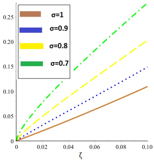
Figure 1. Graphical behavior of our method solution at several values of $\sigma$ for problem 1.

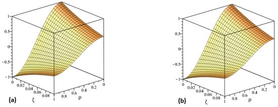
Figure 2. Graphs demonstrating the precise and our approximate solution for problem 2.

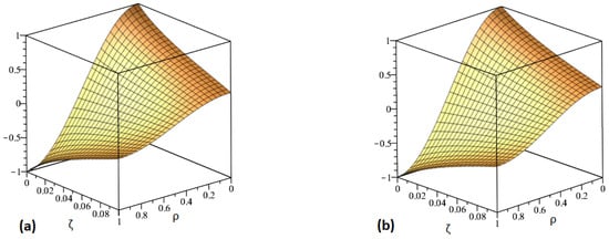
Figure 3. The analytical solution at $\sigma =0.8,0.6$ for problem 2.

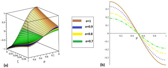
Figure 4. The approximate solution behavior at numerous orders of $\sigma$ for problem 2.

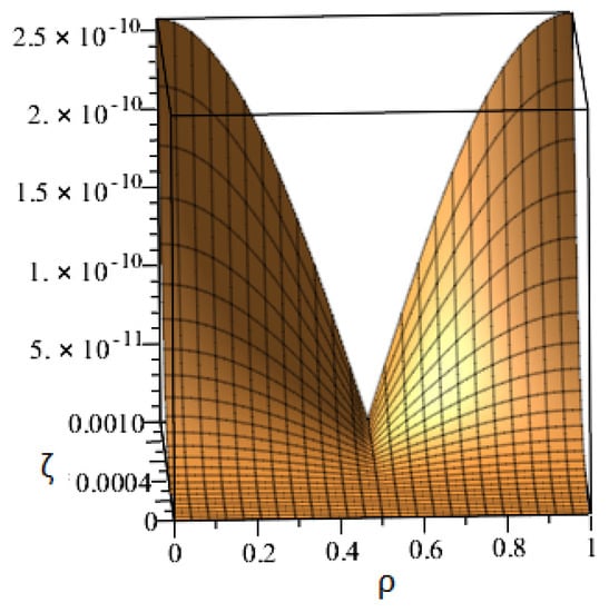
Figure 5. The approximate solution behavior in terms of absolute error for problem 2.

Table 1. Solution of our methods at numerous values of $\sigma$ in comparison with the exact solution for the problem 1.

$\mathit{\zeta }$	$\mathit{\sigma }=0.97$	$\mathit{\sigma }=0.98$	$\mathit{\sigma }=0.99$	$\mathit{\sigma }=1 \left(\mathit{appro}\right)$	$\mathit{\sigma }=1 \left(\mathit{exact}\right)$
0.01	0.0117633	0.0111807	0.0106265	0.0100996	0.0101003
0.02	0.0233010	0.0222901	0.02132284	0.0203973	0.0204026
0.03	0.0349031	0.0335108	0.0321742	0.0308910	0.0309087
0.04	0.0466235	0.0448768	0.0431960	0.0415786	0.0416204
0.05	0.0584848	0.0564017	0.0543938	0.0524583	0.0525394
0.06	0.0704987	0.0680924	0.0657699	0.0635280	0.0636673
0.07	0.0826713	0.0799523	0.0773249	0.0747856	0.0750055
0.08	0.0950063	0.0919829	0.0890584	0.0862293	0.0865554
0.09	0.1075054	0.1041847	0.1009698	0.0978570	0.0983183
0.10	0.1201692	0.1165574	0.1130578	0.1096666	0.1102951

Table 2. Our methods comparison in terms of absolute error at numerous values of $\sigma$ for problem 1.

$\mathit{\zeta }$	$\mathit{\sigma }=0.97$	$\mathit{\sigma }=0.98$	$\mathit{\sigma }=0.99$	$\mathit{\sigma }=1 (\mathit{Our}$  $\mathit{M}\mathit{e}\mathit{t}\mathit{h}\mathit{o}\mathit{d}\mathit{s})$
0.01	1.6630475000$\times {10}^{-03}$	1.0803709000$\times {10}^{-03}$	5.2626840000$\times {10}^{-04}$	6.6320000000$\times {10}^{-07}$
0.02	2.8984310000$\times {10}^{-03}$	1.8874953000$\times {10}^{-03}$	9.2023270000$\times {10}^{-04}$	5.2784000000$\times {10}^{-06}$
0.03	3.9944519000$\times {10}^{-03}$	2.6021760000$\times {10}^{-03}$	1.2655523000$\times {10}^{-03}$	1.7718500000$\times {10}^{-05}$
0.04	5.0031309000$\times {10}^{-03}$	3.2563895000$\times {10}^{-03}$	1.5756267000$\times {10}^{-03}$	4.1764800000$\times {10}^{-05}$
0.05	5.9454599000$\times {10}^{-03}$	3.8623348000$\times {10}^{-03}$	1.8544374000$\times {10}^{-03}$	8.1101800000$\times {10}^{-05}$
0.06	6.8314089000$\times {10}^{-03}$	4.4251796000$\times {10}^{-03}$	2.1026386000$\times {10}^{-03}$	1.3931020000$\times {10}^{-04}$
0.07	7.6658381000$\times {10}^{-03}$	4.9468430000$\times {10}^{-03}$	2.3193742000$\times {10}^{-03}$	2.1986200000$\times {10}^{-04}$
0.08	8.4508834000$\times {10}^{-03}$	5.4275280000$\times {10}^{-03}$	2.5030175000$\times {10}^{-03}$	2.1986200000$\times {10}^{-04}$
0.09	9.1871024000$\times {10}^{-03}$	5.8664606000$\times {10}^{-03}$	2.6515311000$\times {10}^{-03}$	4.6130060000$\times {10}^{-04}$
0.10	9.8740913000$\times {10}^{-03}$	6.2622887000$\times {10}^{-03}$	2.7626624000$\times {10}^{-03}$	6.2853000000$\times {10}^{-04}$

Table 3. Comparison of accurate, our methods and fractional decomposition method (FDM) at numerous values of $\sigma$ for problem 1.

$\mathit{\zeta }$	$\mathit{\sigma }=1 \left(\mathit{FDM}\right)$	$\mathit{\sigma }=1 (\mathit{Our}$  $\mathit{Solution})$	$\mathit{\sigma }=1 \left(\mathit{exact}\right)$
0.2	0.241863	0.2419356	0.2419768
0.4	0.564371	0.564371	0.564371
0.6	0.926696	0.9473451	0.9535662
0.8	1.2210187	1.3022465	1.3463637
1	1.2555556	1.5464218	1.6894984

Table 4. Solution of our methods at numerous values of $\sigma$ in comparison with exact solution for problem 2.

$\mathit{\zeta }$	$\mathit{\rho }$	$\mathit{\sigma }=0.97$	$\mathit{\sigma }=0.98$	$\mathit{\sigma }=0.99$	$\mathit{\sigma }=1 \left(\mathit{appro}\right)$	$\mathit{\sigma }=1 \left(\mathit{exact}\right)$
	0.2	0.80012960	0.80075271	0.80133290	0.80187306	0.80187306
	0.4	0.30562231	0.30586031	0.30608193	0.30628825	0.30628825
0.001	0.6	−0.30562231	−0.30586031	−0.30608193	−0.30628825	−0.30628825
	0.8	−0.80012960	−0.80075271	−0.80133290	−0.80187306	−0.80187306
	1	−0.98901458	−0.98978478	−0.99050194	−0.99116961	−0.99116961
	0.2	0.79170247	0.79279857	0.79382716	0.79479221	0.79479221
	0.4	0.30240343	0.30282210	0.30321499	0.30358361	0.30358361
0.002	0.6	−0.30240343	−0.30282210	−0.30321499	−0.30358361	−0.30358361
	0.8	−0.79170247	−0.79279857	−0.79382716	−0.79479221	−0.79479221
	1	−0.97859807	−0.97995292	−0.98122433	−0.98241720	−0.98241720
	0.2	0.78349599	0.78500661	0.78643103	0.78777387	0.78777389
	0.4	0.29926883	0.29984584	0.30038992	0.30090284	0.30090285
0.003	0.6	−0.29926883	−0.29984584	−0.30038992	−0.30090284	−0.30090285
	0.8	−0.78349599	−0.78500661	−0.78643103	−0.78777387	−0.78777389
	1	−0.96845430	−0.97032153	−0.97208222	−0.97374206	−0.97374208
	0.2	0.77545904	0.77734473	0.77912922	0.78081749	0.78081754
	0.4	0.29619899	0.29691926	0.29760088	0.29824574	0.29824576
0.004	0.6	−0.29619899	−0.29691926	−0.29760088	−0.29824574	−0.29824576
	0.8	−0.77545904	−0.77734473	−0.77912922	−0.78081749	−0.78081754
	1	−0.95852009	−0.96085093	−0.96305669	−0.96514349	−0.96514356
	0.2	0.76756672	0.76979715	0.77191401	0.77392249	0.77392262
	0.4	0.29318439	0.29403634	0.29484491	0.29561208	0.29561213
0.005	0.6	−0.29318439	−0.29403634	−0.29484491	−0.29561208	−0.29561213
	0.8	−0.76756672	−0.76979715	−0.77191401	−0.77392249	−0.77392262
	1	−0.94876464	−0.95152160	−0.95413820	−0.95662081	−0.95662097

Table 5. Our methods comparison in terms of absolute error at numerous values of $\sigma$ for problem 2.

$\mathit{\zeta }$	$\mathit{\rho }$	$\mathit{\sigma }=0.97$	$\mathit{\sigma }=0.98$	$\mathit{\sigma }=0.99$	$\mathit{\sigma }=1 (\mathit{our}$  $\mathit{methods})$
	0.2	1.7434566980$\times {10}^{-03}$	1.1203520100$\times {10}^{-03}$	5.4015897040$\times {10}^{-04}$	2.4887036000$\times {10}^{-10}$
	0.4	6.6594113380$\times {10}^{-04}$	4.2793636670$\times {10}^{-04}$	2.0632227420$\times {10}^{-04}$	7.1909120000$\times {10}^{-11}$
0.001	0.6	6.6594113370$\times {10}^{-04}$	4.2793636670$\times {10}^{-04}$	2.0632227410$\times {10}^{-04}$	7.1889170000$\times {10}^{-11}$
	0.8	1.7434566980$\times {10}^{-03}$	1.1203520100$\times {10}^{-03}$	5.4015897040$\times {10}^{-04}$	2.4887043000$\times {10}^{-10}$
	1	2.1550309300$\times {10}^{-03}$	1.3848311870$\times {10}^{-03}$	6.6767309250$\times {10}^{-04}$	2.5398240000$\times {10}^{-10}$
	0.2	3.0897393450$\times {10}^{-03}$	1.9936424780$\times {10}^{-03}$	9.6505410690$\times {10}^{-04}$	3.3344425000$\times {10}^{-09}$
	0.4	1.1801754450$\times {10}^{-03}$	7.6150373880$\times {10}^{-04}$	3.6861785540$\times {10}^{-04}$	1.3363029000$\times {10}^{-09}$
0.002	0.6	1.1801753450$\times {10}^{-03}$	7.6150363870$\times {10}^{-04}$	3.6861785530$\times {10}^{-04}$	1.2362432000$\times {10}^{-09}$
	0.8	3.0897393450$\times {10}^{-03}$	1.9936424780$\times {10}^{-03}$	9.6505410690$\times {10}^{-04}$	3.3344432000$\times {10}^{-09}$
	1	3.8191279000$\times {10}^{-03}$	2.4642776790$\times {10}^{-03}$	1.1928724030$\times {10}^{-03}$	4.0963790000$\times {10}^{-09}$
	0.2	4.2779009930$\times {10}^{-03}$	2.7672817740$\times {10}^{-03}$	1.3428544530$\times {10}^{-03}$	1.6865120000$\times {10}^{-08}$
	0.4	1.6340127410$\times {10}^{-03}$	1.0570075210$\times {10}^{-03}$	5.1292469100$\times {10}^{-04}$	6.4161661000$\times {10}^{-09}$
0.003	0.6	1.6340127410$\times {10}^{-03}$	1.0570075210$\times {10}^{-03}$	5.1292469090$\times {10}^{-04}$	6.4160675000$\times {10}^{-09}$
	0.8	4.2779009930$\times {10}^{-03}$	2.7672817740$\times {10}^{-03}$	1.3428544530$\times {10}^{-03}$	1.6865021000$\times {10}^{-08}$
	1	5.2877764040$\times {10}^{-03}$	3.4205484070$\times {10}^{-03}$	1.6598593230$\times {10}^{-03}$	2.0798005000$\times {10}^{-08}$
	0.2	5.3585006810$\times {10}^{-03}$	3.4728074860$\times {10}^{-03}$	1.6883158060$\times {10}^{-03}$	5.3049146000$\times {10}^{-08}$
	0.4	2.0467651110$\times {10}^{-03}$	1.3264945210$\times {10}^{-03}$	6.4487930270$\times {10}^{-04}$	2.0334624000$\times {10}^{-08}$
0.004	0.6	2.0467651110$\times {10}^{-03}$	1.3264944210$\times {10}^{-03}$	6.4487920250$\times {10}^{-04}$	2.0234327000$\times {10}^{-08}$
	0.8	5.3585006810$\times {10}^{-03}$	3.4728074860$\times {10}^{-03}$	1.6883158060$\times {10}^{-03}$	5.3048948000$\times {10}^{-08}$
	1	6.6234710410$\times {10}^{-03}$	4.2926261310$\times {10}^{-03}$	2.0868731080$\times {10}^{-03}$	6.5529636000$\times {10}^{-08}$
	0.2	6.3559053610$\times {10}^{-03}$	4.1254748570$\times {10}^{-03}$	2.0086060680$\times {10}^{-03}$	1.2929489000$\times {10}^{-07}$
	0.4	2.4277398400$\times {10}^{-03}$	1.5757912050$\times {10}^{-03}$	7.6721922090$\times {10}^{-04}$	4.9314639000$\times {10}^{-08}$
0.005	0.6	2.4277398400$\times {10}^{-03}$	1.5757912040$\times {10}^{-03}$	7.6721922050$\times {10}^{-04}$	4.9414145000$\times {10}^{-08}$
	0.8	6.3559053600$\times {10}^{-03}$	4.1254748570$\times {10}^{-03}$	2.0086060680$\times {10}^{-03}$	1.2929490000$\times {10}^{-07}$
	1	7.8563310430$\times {10}^{-03}$	5.0993674070$\times {10}^{-03}$	2.4827735950$\times {10}^{-03}$	1.5976180000$\times {10}^{-07}$

7. Conclusions

The ETDM and the HPTM are two unique methodologies that have been thoroughly examined in this work for solving various types of fractional PDEs. The suggested approaches are the combined form of the Elzaki transformation with the Adomian decomposition method and the homotopy perturbation approach. Different dynamics for various fractional orders of the derivative are provided by the fractional-order solutions. In comparison to numerical studies, which require more complex computations, the task can be completed quite simply and effectively using analytical solutions. After all, the researchers can now choose the fractional-order issue whose solution is comparable and extremely close to the experimental results of any physical problem. The identical solutions under the Caputo operator are seen, confirming the important dynamics of the offered problems. Numerical simulation and the graphical behavior of the model are presented to show the reliability of the implemented analytical technique. A comparative analysis of exact and approximate solutions is also presented. The calculated study results have been displayed in tables and graphs. The tables and graphs demonstrate that the approximate solution to the problems converges to the precise solution when the value of $\sigma$ approaches the classical value 1 of the problems. The remarkable results show how simple and effective these approaches are and how they may be applied to other nonlinear problems. Thus, the expansion will be significantly valued to add other operators and approaches in the future, especially in light of the advantages of the current operator. The offered strategies were determined to be suitable to address any physical problem that arises in engineering and the sciences because of their straightforward operation.

References

- Ross, B. (Ed.) Fractional Calculus and Its Applications: Proceedings of the International Conference Held at the University of New Haven, June 1974 (Vol. 457); Springer: Berlin, Germany, 2006. [Google Scholar]
- Yavuz, M. Characterizations of two different fractional operators without singular kernel. Math. Model. Nat. Phenom. 2019, 14, 302. [Google Scholar] [CrossRef]
- Hilfer, R. Threefold introduction to fractional derivatives. In Anomalous Transport: Foundations and Applications; Wiley: New York, NY, USA, 2008; pp. 17–73. [Google Scholar]
- Chaurasiya, V.; Rai, K.N.; Singh, J. Legendre wavelet residual approach for moving boundary problem with variable thermal physical properties. Int. J. Nonlinear Sci. Numer. Simul. 2022, 23, 957–970. [Google Scholar]
- Ganie, A.H.; Houas, M.; AlBaidani, M.M.; Fathima, D. Coupled system of three sequential Caputo fractional differential equations: Existence and stability analysis. Math. Methods Appl. Sci. 2023. [Google Scholar] [CrossRef]
- Harris, P.J. The mathematical modelling of the motion of biological cells in response to chemical signals. In Computational and Analytic Methods in Science and Engineering; Birkhäuser: Cham, Switzerland, 2020; pp. 151–171. [Google Scholar]
- Yazgan, T.; Ilhan, E.; Çelik, E.; Bulut, H. On the new hyperbolic wave solutions to Wu-Zhang system models. Opt. Quantum Electron. 2022, 54, 1–19. [Google Scholar] [CrossRef]
- Tazgan, T.; Celik, E.; Gülnur, Y.E.L.; Bulut, H. On Survey of the Some Wave Solutions of the Non-Linear Schrödinger Equation (NLSE) in Infinite Water Depth. Gazi Univ. J. Sci. 2023, 36, 819–843. [Google Scholar] [CrossRef]
- Zhang, X.; Zhu, H.; Kuo, L.H. A comparison study of the LMAPS method and the LDQ method for time-dependent problems. Eng. Anal. Bound. Elem. 2013, 37, 1408–1415. [Google Scholar] [CrossRef]
- Wang, H.; Yamamoto, N. Using a partial differential equation with Google Mobility data to predict COVID-19 in Arizona. arXiv 2020, arXiv:2006.16928. [Google Scholar] [CrossRef]
- Viguerie, A.; Lorenzo, G.; Auricchio, F.; Baroli, D.; Hughes, T.J.; Patton, A.; Reali, A.; Yankeelov, T.E.; Veneziani, A. Simulating the spread of COVID-19 via a spatially-resolved susceptible-exposed-infected-recovered-deceased (SEIRD) model with heterogeneous diffusion. Appl. Math. Lett. 2021, 111, 106617. [Google Scholar] [CrossRef]
- Ahmed, J.J. Designing the shape of corona virus using the PDE method. Gen. Lett. Math. 2020, 8, 75–82. [Google Scholar] [CrossRef]
- Mastoi, S.; Ganie, A.H.; Saeed, A.M.; Ali, U.; Rajput, U.A.; Mior Othman, W.A. Numerical solution for two-dimensional partial differential equations using SM’s method. Open Phys. 2022, 20, 142–154. [Google Scholar] [CrossRef]
- Al-Habahbeh, A. Exact solution for commensurate and incommensurate linear systems of fractional differential equations. J. Math. Comput. Sci. 2023, 28, 123–136. [Google Scholar] [CrossRef]
- He, H.M.; Peng, J.G.; Li, H.Y. Iterative approximation of fixed point problems and variational inequality problems on Hadamard manifolds. UPB Bull. Ser. A 2022, 84, 25–36. [Google Scholar]
- Yuan, Q.; Kato, B.; Fan, K.; Wang, Y. Phased array guided wave propagation in curved plates. Mech. Syst. Signal Process. 2023, 185, 109821. [Google Scholar] [CrossRef]
- Kilbas, A.A.; Srivastava, H.M.; Trujillo, J.J. Theory and Applications of Fractional Differential Equations; Elsevier: Amsterdam, The Netherlands, 2006; Volume 204. [Google Scholar]
- Podlubnv, I. Fractional Differential Equations; Academic Press: San Diego, CA, USA; Boston, MA, USA, 1999; Volume 6. [Google Scholar]
- Mainardi, F. Fractional Calculus and Waves in Linear Viscoelasticity: An Introduction to Mathematical Models; World Scientific: Singapore, 2022. [Google Scholar]
- Liu, L.; Zhang, S.; Zhang, L.; Pan, G.; Yu, J. Multi-UUV Maneuvering Counter-Game for Dynamic Target Scenario Based on Fractional-Order Recurrent Neural Network. IEEE Trans. Cybern. 2022. [Google Scholar] [CrossRef] [PubMed]
- Cao, Y.; Nikan, O.; Avazzadeh, Z. A localized meshless technique for solving 2D nonlinear integro-differential equation with multi-term kernels. Appl. Numer. Math. 2023, 183, 140–156. [Google Scholar] [CrossRef]
- Akram, T.; Abbas, M.; Ali, A. A numerical study on time fractional Fisher equation using an extended cubic B-spline approximation. J. Math. Comput. Sci 2021, 22, 85–96. [Google Scholar] [CrossRef]
- Srivastava, H.M.; Gusu, D.M.; Mohammed, P.O.; Wedajo, G.; Nonlaopon, K.; Hamed, Y.S. Solutions of general fractional-order differential equations by using the spectral Tau method. Fractal Fract. 2022, 6, 7. [Google Scholar] [CrossRef]
- Bonyadi, S.; Mahmoudi, Y.; Lakestani, M.; Jahangiri Rad, M. Numerical solution of space-time fractional PDEs with variable coefficients using shifted Jacobi collocation method. Comput. Methods Differ. Equ. 2023, 11, 81–94. [Google Scholar]
- Youssri, Y.H.; Abd-Elhameed, W.M.; Ahmed, H.M. New fractional derivative expression of the shifted third-kind Chebyshev polynomials: Application to a type of nonlinear fractional pantograph differential equations. J. Funct. Spaces 2022, 2022, 3966135. [Google Scholar] [CrossRef]
- Sadek, L.; Bataineh, A.S.; Talibi Alaoui, H.; Hashim, I. The Novel Mittag-Leffler-Galerkin Method: Application to a Riccati Differential Equation of Fractional Order. Fractal Fract. 2023, 7, 302. [Google Scholar] [CrossRef]
- Hakkar, N.; Dhayal, R.; Debbouche, A.; Torres, D.F. Approximate Controllability of Delayed Fractional Stochastic Differential Systems with Mixed Noise and Impulsive Effects. Fractal Fract. 2023, 7, 104. [Google Scholar] [CrossRef]
- Youssri, Y.H.; Atta, A.G. Spectral collocation approach via normalized shifted Jacobi polynomials for the nonlinear Lane-Emden equation with fractal-fractional derivative. Fractal Fract. 2023, 7, 133. [Google Scholar] [CrossRef]
- Sunthrayuth, P.; Alyousef, H.A.; El-Tantawy, S.A.; Khan, A.; Wyal, N. Solving fractional-order diffusion equations in a plasma and fluids via a novel transform. J. Funct. Spaces 2022, 2022, 1899130. [Google Scholar] [CrossRef]
- Mishra, N.K.; AlBaidani, M.M.; Khan, A.; Ganie, A.H. Numerical Investigation of Time-Fractional Phi-Four Equation via Novel Transform. Symmetry 2023, 15, 687. [Google Scholar] [CrossRef]
- Owyed, S.; Abdou, M.A.; Abdel-Aty, A.H.; Alharbi, W.; Nekhili, R. Numerical and approximate solutions for coupled time fractional nonlinear evolutions equations via reduced differential transform method. Chaos Solitons Fractals 2020, 131, 109474. [Google Scholar] [CrossRef]
- Fathima, D.; Alahmadi, R.A.; Khan, A.; Akhter, A.; Ganie, A.H. An Efficient Analytical Approach to Investigate Fractional Caudrey-Dodd-Gibbon Equations with Non-Singular Kernel Derivatives. Symmetry 2023, 15, 850. [Google Scholar] [CrossRef]
- Saad Alshehry, A.; Imran, M.; Khan, A.; Shah, R.; Weera, W. Fractional View Analysis of Kuramoto-Sivashinsky Equations with Non-Singular Kernel Operators. Symmetry 2022, 14, 1463. [Google Scholar] [CrossRef]
- Arqub, O.A.; El-Ajou, A. Solution of the fractional epidemic model by homotopy analysis method. J. King Saud Univ.-Sci. 2013, 25, 73–81. [Google Scholar] [CrossRef]
- Song, L.; Zhang, H. Application of homotopy analysis method to fractional KdV-Burgers-Kuramoto equation. Phys. Lett. A 2007, 367, 88–94. [Google Scholar] [CrossRef]
- Alaoui, M.K.; Fayyaz, R.; Khan, A.; Shah, R.; Abdo, M.S. Analytical investigation of Noyes-Field model for time-fractional Belousov-Zhabotinsky reaction. Complexity 2021, 2021, 3248376. [Google Scholar] [CrossRef]
- Zidan, A.M.; Khan, A.; Shah, R.; Alaoui, M.K.; Weera, W. Evaluation of time-fractional Fisher’s equations with the help of analytical methods. Aims Math. 2022, 7, 18746–18766. [Google Scholar] [CrossRef]
- Areshi, M.; Khan, A.; Shah, R.; Nonlaopon, K. Analytical investigation of fractional-order Newell-Whitehead-Segel equations via a novel transform. AIMS Math. 2022, 7, 6936–6958. [Google Scholar] [CrossRef]
- Alyobi, S.; Shah, R.; Khan, A.; Shah, N.A.; Nonlaopon, K. Fractional Analysis of Nonlinear Boussinesq Equation under Atangana-Baleanu-Caputo Operator. Symmetry 2022, 14, 2417. [Google Scholar] [CrossRef]
- Das, S.; Vishal, K.; Gupta, P.K.; Yildirim, A. An approximate analytical solution of time-fractional telegraph equation. Appl. Math. Comput. 2011, 217, 7405–7411. [Google Scholar] [CrossRef]
- Karaagac, B. Two step Adams Bashforth method for time fractional Tricomi equation with non-local and non-singular Kernel. Chaos Solitons Fractals 2019, 128, 234–241. [Google Scholar] [CrossRef]
- Nonlaopon, K.; Alsharif, A.M.; Zidan, A.M.; Khan, A.; Hamed, Y.S.; Shah, R. Numerical investigation of fractional-order Swift-Hohenberg equations via a Novel transform. Symmetry 2021, 13, 1263. [Google Scholar] [CrossRef]
- Sunthrayuth, P.; Ullah, R.; Khan, A.; Shah, R.; Kafle, J.; Mahariq, I.; Jarad, F. Numerical analysis of the fractional-order nonlinear system of Volterra integro-differential equations. J. Funct. Spaces 2021, 2021, 1537958. [Google Scholar] [CrossRef]
- Salama, F.M.; Ali, N.H.M.; Abd Hamid, N.N. Fast O (N) hybrid Laplace transform-finite difference method in solving 2D time fractional diffusion equation. J. Math. Comput. Sci. 2021, 23, 110–123. [Google Scholar] [CrossRef]
- Botmart, T.; Agarwal, R.P.; Naeem, M.; Khan, A.; Shah, R. On the solution of fractional modified Boussinesq and approximate long wave equations with non-singular kernel operators. AIMS Math. 2022, 7, 12483–12513. [Google Scholar] [CrossRef]
- Alderremy, A.A.; Aly, S.; Fayyaz, R.; Khan, A.; Shah, R.; Wyal, N. The analysis of fractional-order nonlinear systems of third order KdV and Burgers equations via a novel transform. Complexity 2022, 2022, 4935809. [Google Scholar] [CrossRef]
- Shah, N.A.; Hamed, Y.S.; Abualnaja, K.M.; Chung, J.D.; Shah, R.; Khan, A. A comparative analysis of fractional-order kaup-kupershmidt equation within different operators. Symmetry 2022, 14, 986. [Google Scholar] [CrossRef]
- Jassim, H.K.; Shareef, M.A. On approximate solutions for fractional system of differential equations with Caputo-Fabrizio fractional operator. J. Math. Comput. Sci. 2021, 23, 58–66. [Google Scholar] [CrossRef]
- Mishra, N.K.; AlBaidani, M.M.; Khan, A.; Ganie, A.H. Two Novel Computational Techniques for Solving Nonlinear Time-Fractional Lax’s Korteweg-de Vries Equation. Axioms 2023, 12, 400. [Google Scholar] [CrossRef]
- Adomian, G. Nonlinear Stochastis System Theory and Applications to Physics; Kluwer Academic Publishers: Dordrecht, The Netherlands, 1989. [Google Scholar]
- Adomian, G. Solving Frontier Problems of Physics: The Decomposition Method; Springer: Dordrecht, The Netherlands, 1994. [Google Scholar]
- Homotopy, H.J. perturbation technique. Comput. Methods Appl. Mech. Eng. 1999, 178. [Google Scholar]
- He, J.H. A coupling method of a homotopy technique and a perturbation technique for non-linear problems. Int. J. Non-Linear Mech. 2000, 35, 37–43. [Google Scholar] [CrossRef]
- He, J.H. Homotopy perturbation method: A new nonlinear analytical technique. Appl. Math. Comput. 2003, 135, 73–79. [Google Scholar] [CrossRef]
- Elzaki, T.M. The new integral transform Elzaki transform. Glob. J. Pure Appl. Math. 2011, 7, 57–64. [Google Scholar]
- Alshikh, A.A.; Mahgob, M.M.A. A comparative study between Laplace transform and two new integrals “Elzaki” transform and “Aboodh” transform. Pure Appl. Math. J 2016, 5, 145–150. [Google Scholar] [CrossRef]
- Elzaki, T.M.; Alkhateeb, S.A. Modification of Sumudu transform “Elzaki transform” and Adomian decomposition method. Appl. Math. Sci. 2015, 9, 603–611. [Google Scholar] [CrossRef]
- Elzaki, T.M. On the connections between Laplace and Elzaki transforms. Adv. Theor. Appl. Math. 2011, 6, 1–11. [Google Scholar]
- Sedeeg, A.K.H. A coupling Elzaki transform and homotopy perturbation method for solving nonlinear fractional heat-like equations. Am. J. Math. Comput. Model 2016, 1, 15–20. [Google Scholar]
- Naeem, M.; Yasmin, H.; Shah, R.; Shah, N.A.; Chung, J.D. A Comparative Study of Fractional Partial Differential Equations with the Help of Yang Transform. Symmetry 2023, 15, 146. [Google Scholar] [CrossRef]
Disclaimer/Publisher’s Note: The statements, opinions and data contained in all publications are solely those of the individual author(s) and contributor(s) and not of MDPI and/or the editor(s). MDPI and/or the editor(s) disclaim responsibility for any injury to people or property resulting from any ideas, methods, instructions or products referred to in the content. |
© 2023 by the authors. Licensee MDPI, Basel, Switzerland. This article is an open access article distributed under the terms and conditions of the Creative Commons Attribution (CC BY) license (https://creativecommons.org/licenses/by/4.0/).