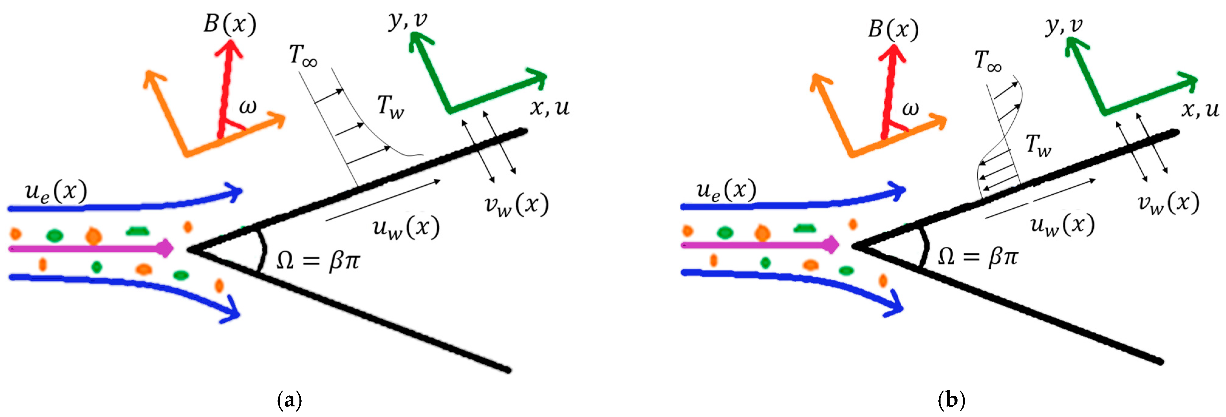
Article

Cubic Chemical Autocatalysis and Oblique Magneto Dipole Effectiveness on Cross Nanofluid Flow via a Symmetric Stretchable Wedge

by
Nor Ain Azeany Mohd Nasir
1,
Tanveer Sajid
2,
Wasim Jamshed
2,*,
Gilder Cieza Altamirano
3,
Mohamed R. Eid
4,5 and
Fayza Abdel Aziz ElSeabee
6,7
1
Department of Mathematics, Centre for Defence Foundation Studies, Universiti Pertahanan Nasional Malaysia, Kem Sungai Besi, Kuala Lumpur 57000, Malaysia
2
Department of Mathematics, Capital University of Science and Technology, Islamabad 44000, Pakistan
3
Universidad Nacional Autónoma de Chota, Cajamarca 06003, Perú-Fizmako Research Group, Bogotá 110110, Colombia
4
Department of Mathematics, Faculty of Science, New Valley University, Al-Kharga 72511, Al-Wadi Al-Gadid, Egypt
5
Department of Mathematics, Faculty of Science, Northern Border University, Arar 1321, Saudi Arabia
6
Mathematics Department, Faculty of Science, Helwan University, Cairo 12612, Egypt
7
Department of Mathematics, College of Science and Arts, Alasyah, Qassim University, P.O. Box 6644, Buraydah 51452, Saudi Arabia
*
Author to whom correspondence should be addressed.
Symmetry 2023, 15(6), 1145; https://doi.org/10.3390/sym15061145
Submission received: 14 March 2023 / Revised: 3 May 2023 / Accepted: 19 May 2023 / Published: 24 May 2023
(This article belongs to the Special Issue Advances in Heat and Mass Transfer with Symmetry)

Abstract

:
Exploration related to chemical processes in nanomaterial flows contains astonishing features. Nanoparticles have unique physical and chemical properties, so they are continuously used in almost every field of nanotechnology and nanoscience. The motive behind this article is to investigate the Cross nanofluid model along with its chemical processes via auto catalysts, inclined magnetic field phenomena, heat generation, Brownian movement, and thermophoresis phenomena over a symmetric shrinking (stretching) wedge. The transport of heat via nonuniform heat sources/sinks, the impact of thermophoretic diffusion, and Brownian motion are considered. The Buongiorno nanofluid model is used to investigate the impact of nanofluids on fluid flow. Modeled PDEs are transformed into ODEs by utilizing similarity variables and handling dimensionless ODEs numerically with the adoption of MATLAB’s developed bvp4c technique. This software performs a finite difference method that uses the collocation method with a three-stage LobattoIIIA strategy. Obtained outcomes are strictly for the case of a symmetric wedge. The velocity field lessens due to amplification in the magneto field variable. Fluid temperature is amplified through the enhancement of Brownian diffusion and the concentration field improves under magnification in a homogeneous reaction effect.

1. Introduction

Since typical fluids exhibit poor thermal conductivity, researchers have concentrated their efforts on studying this issue. Conventional fluids possess low thermal conductivity; this is a considerable obstacle faced by the world today. To solve this problem, nanofluids transport heat into the gap, thus causing it to close. Nanofluids are a distribution of micron-sized particles that, in comparison to typical liquids, measure more than 100 nanometers. The observation that a conventional fluid is submerged within nanoparticles was coined by Choi [1]. Lee et al. [2] participated in a laboratory investigation, and their results revealed that nanoparticle immersion increases heat transmission characteristics. As a result of this study, Buongiorno [3] was able to derive a hypothesis on the mechanism of heat conduction in nanomaterials by assuming thermophoretic dispersion in conjunction with Brownian mobility, allowing him to come to his conclusion. An investigation into the effects of mixed convection and MHD on the flow of nanofluids when they are exposed to an infinite sheet was provided by Reddy et al. [4]. Khan and Pop [5] investigated the effects of nanofluids on thermophoresis and Brownian diffusion effects through an expanding medium and concluded that a nanofluid travels when it is exposed to a flat surface. Their research was published in the journal Nano Letters. Sheikholeslami et al. [6] presented a forecast on the influence that MHD would have on a nanofluid through the inclusion of alumina nanoparticles. The heat transfer effect was effectively examined by Mutuku-Njane and Makinde [7] in the instance of a nanofluid moving through an expanding sheet embedded with Newtonian heating phenomena. Atashafrooz et al. [8] explored the impact of a magnetic field and bleeding on nanofluid flow in a trapezoidal recess. Atashafrooz et al. [9] carried out an entropy generation analysis of a three-dimensional fluid flow accompanied with effects such as a magnetic field and a nanoparticle. Khan et al. [10] scrutinized the behavior of nanoparticles in addition to thermal radiation on a fluid going past an extendable sheet and observed that the heat transfer rate amplifies by magnification of the radiation parameter. Ma et al. [11] investigated the effect of nanoparticles and convective boundary conditions on a fluid flowing through a channel and observed that the temperature profile is amplified by the quantity of nanoparticles. More recently, Saleem al. [12] utilized the magnetic field effect and the natural convection on fluid through an L-shaped enclosure with time-periodic boundary conditions. Saleem et al. [13] investigated the influence of a rotating magnetic field and the free convection effect on a nanofluid considering water as a base fluid flow through a corrugated enclosure. Mahanthesh et al. [14] investigated the impact of nonlinear convection and nonlinear-based thermal radiation on a three-dimensional Maxwell fluid flow subjected to an expandable sheet. Krupalakshmi et al. [15] investigated the influence of dust particles as well as thermal radiation on a magnetized upper-convected moving Maxwell nanofluid while subjected to a convectively heated surface. Khan et al. [16] investigated the influence of nonlinear-based thermal radiation phenomena and microorganisms on a Burgers nanofluid. Gireesha et al. [17] researched the influence of a heat source/sink and a nonlinear radiation phenomenon on a mixed convective Maxwell nanofluid. Irfan et al. [18] studied an Oldroyd-B liquid embedded with a radiation phenomenon and a chemical reaction. The stagnation point effect and nonlinear effect-based thermal radiation consequences on the Oldroyd-B nanofluid were studied in depth by Irfan et al. [19]. Irfan [20] adopted the Buongiorno nanofluid model to investigate the thermophoretic effect on a Maxwell nanofluid moving subjected to an extending sheet accompanied by Joule’s heating effect. Similar work reported by authors is mentioned in [21,22,23,24,25].
In the course of the past few decades, researchers from all over the world have conducted studies regarding the dynamics of fluid motion when it is exposed to a symmetrical wedge. This is due to the variety of uses it has within industry, such as the production of polymer products, oil mining, the delivery of chilled air inside AC panels, nuclear power reactors, the design of aircraft wings to provide maximum lift, the design of warships, the navigation of fighter jets, and the simulation of fluid flows. Falkner [26] researched the impact of boundary layer hypotheses on fluid flow when Falkner’s symmetric wedge modifies the flow. He found that the boundary layer assumptions had a significant impact on the movement of the liquid. They provided the Falkner–Skan equations for the analysis of the fluid flowing through a wedge. As a consequence, this type of wedge was renowned in the time period that followed the presentation of these equations. Haratee [27] developed a computational framework describing the scenario of a fluid reaching a Falkner wedge that corresponded to the boundary layer assumptions. This model was based on observations of the circumstances. Yih [28] provided a study on the effect of forced convection on a Magnus liquid moving under a non-isothermal wedge. His interest was in how the flow was affected. Ishak and colleagues [29] developed a mathematical framework to simulate a situation in which the rate of fluid movement is altered by a moving wedge. The heat source and sink events that might take place in this environment are accounted for by this model. Yacob et al. [30] employed the Falkner–Skan concept to study the effect of a nanofluid that traveled along the direction of a moving wedge. Hashim and Khan [31] conducted studies on the dynamics of a Carreau liquid flow approaching a stationary or movable wedge. They also conducted additional studies involving the heat dispersion phenomenon. In addition, they conducted studies regarding the process of heat diffusion. Xu and Chen [32] investigated how a magnetic field influenced the movement of a liquid across a perforated wedge and how the thickness of the liquid was altered as a result of the magnetic field’s influence. Permeable pores in a medium with a constant wedge allowed Sayyed et al. [33] to obtain an analytical solution of a magnetized fluid moving across a slippery wedge with pores. Awaludin and colleagues [34] were successful in achieving their dual objective of finding a solution for fluid flow while it was subjected to the geometry of expanding and contracting wedges and the impact of heat generation. Both objectives were reached simultaneously. Researchers Ibrahim and Tulu [35] completed an in-depth study on the function of dissipation in viscosity and magnetic influence on a nanofluid as it passed through a wedge and merged with the heat transport phenomenon.
Since many physiologically responsive systems, such as tower cooling, include a combination of heterogeneous and homogeneous (H–H) chemical interactions, these reactions were crucial. This happens because H–H reactions can be endothermic as well as exothermic. A strong connection occurs between most of the fluid’s homogeneous processes and the catalytic surface’s heterogeneous reactions. Surface and liquid temperatures, as well as fluid and reactant species concentrations, interact in triangular fashion. There has been very little research completed on these chemical processes which are relevant to the diffusion and the formation of fog, as can be seen from the references. Merkin [36] constructed a model to explore the influence of catalytic reactions on a boundary layer fluid flow when it was exposed to an expandable medium. The goal of this investigation was to better understand the flow of the boundary layer. The Buongiorno model was used by Xu et al. [37] to investigate the effect of catalysis along with the stagnation point in the case of a nano-liquid that was passed through an elastic medium. Hayat et al. [38] conducted extensive research on the impact of the cubic autocatalytic process with radiation influence on the motion of a nanofluid when it was exposed to a 3D extensible medium. Mtiaz et al. [39] researched the influence of chemical reactions on radiative second grade liquid motion subjected to a curved surface integrated with magnetic phenomena. This study addressed a chemical specie process using a 2nd grade liquid. Waqas [40] designed a mathematical model to study the impact of chemical reactions on ferromagnetic liquids.
The erratic and random migration of nanoparticles in a fluid is referred to as Brownian motion. This term explains the microscopic particles suspended in gas or liquid. Brownian motion was first introduced by Brown [41] when he noticed that pollen grains in the fertilization process represent the rapid, oscillatory migration of nanoparticles; hence, he named this motion Brownian motion. Russel [42] did work on the Brownian motion of small particles which are suspended in liquids. Many researchers used Brownian motion analysis to enhance thermal conductivity. Jan et al. [43] used Brownian motion analysis for improving the thermal conductivity of a nanofluid and proved that the larger migration of random particles helps boost thermal conductivity. Further Rauwerdink et al. [44] analyzed the measurement of molecules of magnetic nanoparticles using Brownian motion.
Thermophoresis or thermos migration is the mixture of nano mobile particles when the force temperature gradient is applied. In thermophoresis, particles move from lower temperature regions to higher temperature regions. Thermophoresis was utilized to analyze the concentration distribution; an existing study reveals that when particles become large, the concentration distribution becomes non-uniform. Many scholars have investigated mass transfer with the effect of thermophoresis. Natural convective heat and mass transport are carried out with thermophoresis and Brownian motion by Pakravan et al. [45]. Dmitriey [46] explored heat and mass transfer in a nanofluid with thermophoresis and Brownian motion. The effect of an interfacial nanolayer nanofluid with thermophoresis is investigated by Fu [47]. Saleem et al. [48] investigated the influence of internal heat generation on rarefied gaseous flow by natural convection heat transmission in a partly heated, square, two-sided, and wavy cavity. Double-diffusion natural convection for staggered cavities with a concave lower wall is investigated in detail by Khalaf et al. [49].

1.1. Purpose of the Current Study

1.1.1. Existing Literature

In the previous studies, each researcher explored the effect of the H–H interaction on fluid flow towards distinct geometric shapes, such as extending discs, channels, cones, and cylindrical objects, and assessed possible solutions to these problems. However, no effort has been made to analyze heat and mass transfer in terms of the fluid flow embedded within H–H reactions moving past a wedge.

1.1.2. Research Gap

Considering the research discussed earlier, it can be said that no effort has been made to investigate the influence of H–H upon a Cross nanofluid moving towards an extensible and additionally shrinkable wedge that is embedded with heat-generating phenomena.

1.1.3. Present Study

The purpose of the current investigation is to explore the heat and mass transport features of a viscous Cross fluid that is traveling through a symmetrically expanding wedge in conjunction with the Buongiorno nanofluid concept and heat-generating phenomena.

1.1.4. Novelty

The article is one of a kind because the effect of H–H reactions of a non-Newtonian liquid through a symmetric extensible wedge has not been examined previously in any other piece of published research in this area.

2. Geometry of the Statement

A two-dimensional Cross nanofluid moves towards a symmetric wedge accompanied by the utilization of an inclined magnetic field of strength B x = B 0 x m 1 / 2 , where B 0 depicts a steady magnetic field. U w x = a x m reflects velocity distribution; a > 0 and a < 0 point to the expansion and contraction of the wedge as shown in Figure 1. Moreover, U x = b x m reflects free stream velocity with constant b ; symbol m indicates the viscosity index. An important part of the Falkner–Skan wedge ranges m 0 ,   1 . In addition, m = β / 2 β , β = Ω / π indicate the wedge angle. Energy transport is carried out with the inclusion of the heat generation phenomenon. Coordinated axes are chosen in a manner that the x -path is adjusted in parallel with the wedge plane and the y -direction is orthogonal to it. The mass transfer phenomenon is studied using the isothermal chemical process and by assuming autocatalysis. Let E and F be auto-catalysts, so autocatalysis in case of the isothermal reaction is
E + 2 F 3 F , a n d   r a t e = k 1 G a G b 2 .
On a catalytic plane, the isotherm reactive fluxing is single order and presented as
E F , a n d   r a t e = k s G a .
It is noted that r a t e = k s G a G b 2 is zero away from the field and influences the edge of the wedge. The term k s , k 1 , is the rate factor of the heterogeneity (homogeneity) reaction; G a , G b is the concentration of the chemical species E , F , separately. The wall, as well as the ambient temperature/concentration of nano-molecules, are denoted by T w , C w , T , C . Buongiorno pioneered convective transport in nanofluids [19]. He claimed that nanofluids are created colloids comprising a base fluid and nanoparticles (ranging in size from 1 to 100 nm). He considered seven different slip processes, including the inertial phenomenon, Brownian dispersion, heat phoresis, the magnetic phenomenon, diffusion phoresis, drainage of the fluid, and buoyancy under the effect of gravity. He claimed that Brownian dispersion is one of the most important slip systems in nanofluids. This mathematical modelling will use the Buongiorno model to solve the free convection problem in nanofluids by only considering the effects of Brownian motion,   D B , which is associated with G b and thermophoresis D T , on flow, heat, and mass transfer from a flat plate with a prescribed surface heat flux. The equation of continuity (3) is based on the law of conservation of mass. Total mass is conserved. The momentum equation (4) is derived through the utilization of Newton’s second law of motion which gives a relationship between force and acceleration of the fluid flow as well as the condition for conserved momentum. The momentum of the system remains constant: momentum can be neither created nor destroyed. The energy equation (5) is based on the principle of conservation of energy which states that energy can be neither created nor destroyed by transfer from one form to another form. The energy equation is derived using the second law of thermodynamics which states that a change in internal energy is equal to heat plus the work completed. Equations (6) and (7) are derived using Fick’s second law of diffusion which examines the rate of change of different concentrations with time at a point in the system. The fluid is moving over an expandable sheet in the horizontal direction, having a velocity component u and a vertical component of velocity v acting along the y -axis, which is 0. Furthermore, it is noted that · v = 0 , and the governing equations are [27,28,29,30,31,32,33,34,35,36,37,38,39,40].
u x + v y = 0 ,
u u x + v u y + σ B 2 x s i n 2 ( ω ) ρ u U U d U d x = υ y u y 1 + Γ u y n ,
u T x + v T y = α 2 T y 2 + τ D B T y G b y + T D T 1 T y 2 + Q * T T ρ C p f ,
u G a x + v G a y = D A 2 G a y 2 + k 1 G a G b 2 ,
u G b x + v G b y = D B 2 G b y 2 + D T T 2 T y 2 + k 1 G a G b 2 .
It is assumed that the flow started at y 0 and that the u and v are the velocity along the x - and y -axes, concurrently. The wedge is stretched or shrunk in the direction of the x -axis with velocity U w x . The mass transfer velocity is v w x , where v w > 0 is the injection parameter while v w < 0 is the suction parameter; the ambient velocity is U . Wall temperature is denoted by T w , and the condition T = T w is with surface temperature. Initial conditions at the surface of the sheet in case of homogeneous/heterogeneous reactions are D A G a y = k s G a , D B G b y = k s G b , whereas free stream temperature is denoted by boundary T . The free stream concentration in terms of G a and G b at the boundary is given by G a G and G b G . Boundary layer approximation is used in the case of free stream velocity, temperature, and concentration.
The BCs are enumerated below [27,28,29,30,31,32,33,34,35,36,37,38,39,40].
u = U w x , v = v w x , T = T w , D A G a y = k s G a , D B G b y = k s G b   at   y = 0 , u U , G a G , T T , G b G ,   a s   y .
Equation (3) is automatically satisfied as equal to zero by utilizing the similarity transformation. Equation (4) comprises the inclined magnetic field which produces a Lorentz force that provides resistance to the fluid flow, i.e., the Falkner–Skan wedge term, a Cross fluid in which Γ indicates a material constant and n represents the viscosity index. The terms on the right-hand side of Equation (5) indicate thermal diffusivity, a Buongiorno nanofluid having the combination of Brownian diffusion D B and thermophoresis parameter D T ; species diffusivity of chemical species a is represented by G a ; and Q * depicts heat generation. In Equations (6) and (7), the first terms on the right-hand side indicate the diffusion equations of the chemical species. Velocity components = u , v ; ρ = density of based fluid; electric conductance = σ ; kinematic viscosity = υ ; the relaxing time is = Γ ; the consistency factor = n ; c p = heat capacitance; τ = ρ c n a n o p a t r i c l e s ρ c b a s e f l u i d = ratio of heating capacitance (effective) of nanomolecules and a conventional liquid; the Brownian coefficient = D B and D T = diffusion of thermophoresis/species F . Mass flux time-dependent velocity takes the form v w x = v 0 x 1 m 2 , and heat generating/absorption takes the form of Q * = Q 0 / x 1 m . Q 0 is a constant coefficient of energy generation/absorption; β 0 is volume thermal expansion.

Assumptions

  • Modeled Equations (3)–(7) are developed from the principle of preservation of mass, the 2nd law of motion, the 2nd law in the case of energy investigation, and Fick’s 2nd law of concentration in the case of mass diffusion analysis.
  • The density of the fluid does not vary (incompressible) and flows smoothly (laminar).
  • The influence of the inclined magnetism force is considered to investigate the magnetic Lorentz force on fluid flow subjected to a wedge.
  • The Buongiorno nanofluid type is deemed to investigate the effect of the nanofluid on the Cross fluid.

3. Transformation

The appropriate conversions are listed below [27,28,29,30,31,32]:
η = y U m + 1 2 ν f x m 1 / 2 ,   T w T θ η + T = T , G a = G ϕ η , G b = G φ η .
Expressions regarding velocity components u and v are given by u = U x m d f d η , v = ( 1 + m ) v f U 2 1 2 x m 1 2 f η + m 1 m + 1 η d f d η . After employing Equation (9), the governing PDEs are renovated into the ODEs enumerated below [27,28,29,30,31,32,33,34,35,36,37,38,39,40].
1 + W e n d 2 f d η 2 n 2 1 + 1 n W e n d 2 F d η 2 n f + f d 2 f d η 2 + 2 m m + 1 1 d f d η 2 M 2 s i n 2 ( ω ) 1 d f d η = 0 .  
d 2 θ d η 2 + P r f d θ d η + N b d θ d η d φ d η + N t d θ d η 2 + Q θ = 0 ,
d 2 ϕ d η 2 + S c f d ϕ d η + k 2 ϕ φ 2 = 0 .
1 δ S c d 2 φ d η 2 + N t N b θ + f d ϑ d η + k 2 ϕ φ 2 = 0 .
Taking D A = D B , we obtain δ = 1 . Employing ϕ + φ = 1 [50] above, (11)–(12) take the form
d 2 ϕ d η 2 N t N b d 2 θ d η 2 + S c f d ϕ d η S c k 2 ϕ ( 1 ϕ ) 2 = 0 .
The transformed BCs are
f 0 = f w , d f 0 d η = ε ,   θ 0 = 1 , d ϕ d η 0 = ε 1 ϕ 0 , d f 0 d η 1 , θ 0 , ϕ 1 .
After utilizing similarity transformations, Equation (4), referred to as the momentum equation, is transformed into Equation (10). The energy equation (5) is transformed into the ODE mentioned in Equation (11), and the homogeneous/heterogeneous modeled PDEs (6) and (7) are transformed into the ODEs mentioned in Equations (12) and (13) after utilizing similarity transformations. Here ( ε > 0 ) and ( ε < 0 ) reflect extensible as well as contractable wedge cases. Sundry parameters are the magnetic effect M 2 = 2 σ B 0 2 x m 1 ρ b m + 1 ; the Weissenberg number (local) is W e 2 = 1 2 υ x 3 m 1 Γ m + 1 b 3 ; the intake/outtake effect is f w = 2 σ ρ b m + 1 ; and ε 1 = 2 υ b m + 1 x 1 m k s D A is the diffusion coefficient. Further, the Brownian motion parameter is N b = τ D B G ν ; the thermophoresis parameter is N t = τ D T T w T ν T ; the heat generation parameter is Q = Q 0 b m + 1 ρ c p ; the Schmidt number S c = υ D B ; and k 2 = 2 k 1 G x m 1 m + 1 is the homogeneous reaction with a coefficient rate k 1 . The term δ = D A D B is the ratio of species diffusivity. The final form of the Weissenberg number obtained by taking m = 1 / 3 is W e 2 = 2 Γ b 3 3 υ x 2 .
Physical quantities of interest, such as the drag friction and the Nusselt number, are enumerated below [27,28,29,30,31,32,33,34,35,36,37,38,39,40].
C f x = [ τ w ρ U w 2 ] , N u x = [ x q w k ( T w T ) ] , S h x = [ x q m D B ( C w C ) ] , ( R e x ) 0.5 C f x = [ ( m + 1 ) 2 ] d 2 f ( 0 ) d η 2 { 1 [ 1 + ( w e d 2 F ( 0 ) d η 2 ) n ] } , ( R e x ) 0.5 N u x = [ ( m + 1 ) 2 ] { d d η [ θ ( 0 ) ] } , ( R e x ) 0.5 S h x = [ ( m + 1 ) 2 ] d d η [ ϕ ( 0 ) ] ,
where R e = b x m + 1 υ , C f x , and N u x are the Reynolds numbers that have a ratio of inertial forces to viscous forces, skin friction, and the Nusselt number, respectively.

4. Numerical Solution

4.1. Explanation of the bvp4c Scheme

We utilized MATLAB’s bvp4c technique. This software performs a finite difference method that uses the collocation method with three stages of the LobattoIIIA strategy.
The collocation schemes in the case of two-point BVP are given by
x = Ψ t , x ,   L t M ,
having BCs
B C x L ,   x M = 0 .
The estimated solution U(t) seems to be a constant value that constitutes a cubed polynomial upon every sampling period [ t n , t n + 1 ] of a grid L = t 0 < t 1 < t 2 < t 3 < t N = M . The boundary criteria are met by this solution.
B C U L ,   U M = 0 .
It fulfills (collocates) the DE across both endpoints of each subinterval, in addition to the midway for every subinterval:
U t n = Ψ t n , U t n = 0 , U t n + t n + 1 2 = Ψ t n + t n + 1 2 , U t n + t n + 1 2 = 0 , U t n + 1 = Ψ   t n + 1 , U t n + 1 = 0 .
Based on these restrictions, a whole set of algebraic equations is made to describe the coefficients that make up U t . These equations then need to be linearized so that they can be evaluated iteratively. In this case, U t is an estimate of a single response x t to a fourth degree. It can be written as x t U t Z Ω 1 4 , where Ω 1 = t n + 1 t n is the maximum number of measurements and Z is a constant value. Based on this estimate, the following is a definition of the remnant r x in all of ODE:
r t = U   t Ψ t , U t .
The level of tolerance for this particular instance of the issue is 10 6 , and the range of calculation is [0, 7] instead of [0, ].

4.2. Bvp4c Numerical Scheme for the Present Problem

For the numerical process, we used the shooting method, which handled the boundary condition problem and converted these into an initial value problem so that the bvp4c technique can process further on a system of ODEs. The analytical and MATLAB procedures [51] are below.
R 1 = f , R 2 = d f d η , R 3 = d 2 f d η 2 , R 4 = θ , R 5 = d θ d η , R 6 = ϕ , R 7 = d ϕ d η , R 8 = φ , R 9 = d φ d η ,
d R 3 d η = 1 T e r m 1 [ ( 1 + W e n ( R 3 ) n ) 2 + R 1 R 3 + 2 m ( m + 1 ) [ 1 ( R 2 ) 2 ] M 2 [ 1 ( R 2 ) ] ] , d R 5 d η = P r [ R 1 R 5 + N b R 5 R 7 + N t ( R 5 ) 2 + Q R 4 ] , d R 7 d η = S c [ R 1 R 6 + k 2 R 6 ( 1 R 6 ) ] N t N b d R 5 d η , d R 9 d η = S c [ R 1 R 8 + k 2 R 8 ( 1 R 8 ) ] N t N b d R 5 d η .
T e r m 1 = 1 + 1 n W e n R 3 n .  
R 1 0 = f w , R 2 0 = ε , R 4 0 = 1 , N b R 6 0 + N t R 5 0 = 0 , R 9 0 = ε 1 R 8 0 , R 2 1 , R 4 0 , R 6 1 , R 8 0 0 .
The back of bvp4c is the R-K45 numerical method which is the most convergent for solving the first-order linear/nonlinear ODEs. This method is also known as the collection procedure of order four. This numerical strategy must choose the finite and approximate value of η , in this case, η = 8 . The convergence criterion has been achieved in the case of η = 8 for the case of momentum, temperature, and concentration equations with the crude mesh of 120 points taken during the numerical simulation of the problem. The MATLAB programming procedure is also given here. Figure 2 is designed to represent the mechanism of the bvp4c scheme.

4.3. Pseudo Code of the Proposed Scheme

  • Clear the command window and all variables
  • Set the desired display format to “long”
  • Set the values of the variables:
    We = 0.1; M = 0.1; omega = 1.5; m = 0.5; n = 0.5; Pr = 0.7; Nb = 0.5; Nt = 0.5; Q = 0.1; Sc = 1; K2 = 1; fw = 1; epsilon = 0.2; epsilon1 = 0.2;
  • Set the value of “infinity” to 7
  • Initialize the solution structure “solinit” using bvpinit function with the following arguments:
    a.
    A vector of 170 equally spaced values ranging from 0 to “infinity”
    b.
    A column vector of zeros of size 7 × 1
  • Set the options for the bvp4c function using bvpset with the following properties:
    a.
    Stats: on
    b.
    RelTol: 1 × 10⁻⁶
  • Define the cell array “lines” with the following string values:
    a.
    ‘k’
    b.
    ‘r’
    c.
    ‘b-’
    d.
    ‘g’
  • Solve the boundary value problem four times using the bvp4c function with the following arguments:
    a.
    ex8ode—ODE function
    b.
    ex8bc—Boundary conditions function
    c.
    solinit—Initial guess for the solution
    d.
    options—Options structure created in step 6
    e.
    We, M, omega, m, n, pr, Nb, Nt, Q, Sc, K2, fw, epsilon, and epsilon1—values defined in step 3
    f.
    Store the solutions in the variables sol1, sol2, sol3, and sol4, respectively.
  • Compute the following expression:
    (m + ½)(sol1.y(3,1))(1 + We^2*(sol1.y(3,1))^2)^(n − ½), −1*(m + ½)sol1.y(5,1),
    1(m + ½)*sol1.y(7,1)
  • Create three figures and plot the solutions using the plot function with following arguments:
    a.
    sol1.x, sol1.y(2,:), lines{1}
    b.
    sol2.x, sol2.y(2,:), lines{2}
    c.
    sol3.x, sol3.y(2,:), lines{3}
    d.
    sol4.x, sol4.y(2,:), lines{4}
    e.
    Set the following: i. LineWidth: 2 ii. MarkerSize: 8
    f.
    Label the y-axis and x-axis accordingly
    g.
    Use the “hold on” command to allow multiple plots in the same figure
  • Repeat step 10 for the other two figures, plotting the appropriate solutions and labeling the y-axis and x-axis accordingly
  • Open the command window and show the plots using the “shg” command
  • Define the ODE function “ex8ode” with the following arguments:
    a.
    x: independent variable
    b.
    y: column vector of dependent variables
    c.
    We, M, omega, m, n, Pr, Nb, Nt, Q, Sc, K2, fw, epsilon.

5. Value of f 0 with Variation of ε

The value of f 0 is checked by both routines: the bvp4c/shooting method for computing with fixing parameters and giving variation to ε (wedge stretching/shrinking parameter) and tabulated in Table 1. Both techniques bring the same findings which show the accuracy of this result.

6. Entropy Generation

The mathematical form of entropy is changed by
E g = k f T 2 T x 2 + T y 2 + μ f T u y 2 + σ B 2 s i n 2 ω u 2 T + R D A C G a y 2 + D A T T y G a y .
The first expression relates to heat irreversibility. Fluid friction can be represented mathematically in the second term; the third expression indicates the magnetic effect; mass transport is illustrated in the fourth term; and the combined effect of heat and mass expressions are represented in the last term. Entropy generation can be expressed as
N g = E g k f / x 2 Ω T 2 .
Dimensionless entropy generation is enumerated below.
N g = N g h + N g f + N g M + N g m + N g h m   .  
The expressions N g h ,   N g f ,   N g M ,   N g m ,   N g h m in a previous formula symbolize the generated entropy by heat transfer, liquid frictions, the Magnus effect, and mass transfer; the term comprises both mass and heat transportation and is enumerated below.
N g h = m + 1 2 R e x θ 2 ,   N g f = m + 1 2 B r Ω T R e x f 2 , N g M = M B r Ω T R e x f 2 ,   N g m = m + 1 2 M m Ω C Ω T 2 R e x ϑ 2 , N g h m = m + 1 2 M m Ω C Ω T R e x θ ϑ ,
whereas
B r = μ f u e 2 k f T w T , R e x = u e x v f ,   Ω T = T w T T ,   Ω c = C w C C ,   M m = R D B C k f .

7. Results and Discussion

This segment develops the resulting impact of various parameters on the movement, temperature, and concentration distribution of the Cross nanofluid. All related figures show the impact of the magnetic parameter M , suction/injection f w , and the Weissenberg number W e on the movement of a Cross nanofluid for both cases of a shrinking ( ε < 0 ) /stretching ( ε > 0 ) wedge. The analysis of temperature visibility is visible in the Brownian factor N b , the thermophoresis variable N t , the heat generative variable Q , the Schmidt number S c , and the strength coefficient of homogeneous reaction k 2 . Another important aspect of this examination is the scrutiny of the concentration profile which is taken with catalyst species and a higher rate of chemical homogeneous/heterogeneous reaction. The effect of various dimensional parameters on drag friction and the Nusselt number are shown in Table 2. From Table 2, it is observed that the heat transfer Nusselt number is amplified as a result of an incremental change in the sundry dimensionless parameters, such as the Prandtl number P r , the diffusion coefficient ε 1 , the inclined angle ω , and heat generation Q and ε . However, the heat transfer rate diminishes by improving the magnetic parameter M , the strength of the homogenous reaction k 2 , the Brownian diffusion N b , the thermophoresis diffusion N t , the Schmidt number S c , and f w . The Sherwood number magnifies by augmenting P r , N t , ε 1 , ω , and Q , but it diminishes by escalating M , k 2 ,   N b , and S c , ε , and f w . The dimensionless parameters used in this study range between 0 W e 2 , 0 M 1.5 , 0 k 2 2 , 0 P r 3 , 0 N b 2 , 0 N t 1.5 , 0 S c 1.5 , 0 ε 1 1 , 0 ω π 3 , 0 Q 2.5 , 0 ε 1 , 0 f w 1 . Table 3 is designed to study the impact of Prandtl numbers P r and Q on the Nusselt number in the presence/absence of the nanofluid. It is observed that the relative error is small in the case of P r = 0.7 and higher in the case of Q = 0.5 .
Figure 3 and Figure 4 describe the impact of W e and M on the velocity of the nanofluid. This graph shows that for a greater W e , the velocity diminishes due to the relaxation time constant in the status of the stretchable wedge. The velocity increases in the status of the shrinkable cylinder due to the shrinking of the wedge, while a greater Cross index n causes a growth of velocity in the shrinking wedge and a decrement in the case of a stretching wedge. For rising values of M and m , velocity falls in the case of a stretching wedge due to the Lorentz force produced as a result of an electrically conducting fluid moving through a magnetic field, which creates an obstacle in the layers of fluid. Growth is detected in the case of a shrinking wedge because shrinkage of the wedge provides a smooth path for the flow. This impact of the viscosity index parameter n and the suction/injection parameter f w on the velocity field is sketched in Figure 5 and Figure 6. It is quite evident that the viscosity in the case of a fluid is amplified by a rising n. The fluid passes relatively across the extensible surface in contrast to the shrinking surface. The viscosity of the fluid diminishes when moving over an expandable surface, which amplifies the velocity field; the situation is quite the opposite in the case of the shrinking wedge which amplifies fluid velocity as shown in Figure 5. It is observed that the velocity decreases sufficiently by improving the suction parameter, and this decrement is more dominant when the fluid is moving over a stretching wedge with ϵ = 0.2 ; this is in contrast to a shrinking wedge case with ϵ = 0.2 . Figure 7 and Figure 8 show a brief description of the temperature profile owing to magnification in Brownian diffusion and the thermophoresis parameter in the case of a stretching/shrinking wedge. It is observed that molecules of the fluid share more kinetic with each other by improving N b and N t , which amplifies the temperature field and heat transfer rate both for the case of the stretching wedge with ϵ = 0.2 and the shrinking wedge with ϵ = 0.2 . It is observed that molecules of the fluid migrate from a colder surface to a hotter surface as a result of the magnification in the thermophoresis parameter which amplifies the temperature of the fluid in light of Newton’s law of cooling and brings about amplification in the temperature field both for the case of ϵ = 0.2 and ϵ = 0.2 . A greater Prandtl number causes lower boundary layer thickness due to the temperature of the nanofluid going down. The Prandtl number is the ratio of momentum diffusivity to thermal diffusivity. Heat disperses quickly by improving Pr, which slows down the temperature inside and the heat transfer for both cases of a stretching/shrinking wedge, as shown in Figure 9. It is observed that the heat generation effect works on the principle of endothermic reaction, where heat is absorbed by the system. More heat is absorbed under magnification in Q . Heat generation is amplified by utilizing a nanofluid which increases liquid temperature whether it is moving over a stretching/shrinking wedge, as shown in Figure 10. When a substantial chemical process is improved by a heterogeneous reaction (reactions that take place across the surface of a separate phase catalyst), the chemical distribution in the flow system is reduced, and the concentration field is amplified, as shown in Figure 11. Figure 12 emphasizes the impact of the Brownian diffusion parameter N b on the concentration field. As shown in Figure 12, the concentration of the fluid drops as N b increases because Brownian motion causes the boundary layer to warm, which in turn causes the particles to leave the fluid regime and weaken the concentration field. The concentration of the fluid decreases due to the rising heterogeneous reaction effect. As in Figure 11, the chemical reaction slows down by a rising K 2 , which diminishes the concentration field. This behavior is for both cases of the stretching/shrinking wedge, as shown in Figure 13. Figure 14 demonstrates the effect of the thermophoresis parameter N t on ϕ η . Molecules of the fluid migrate from a hotter surface to a colder one by increasing the thermophoresis parameter, which improves the chemical reaction process, and, in addition, elevates the concentration field ϕ η .

8. Statistical Measures of Dimensionless Parameters on Drag Friction and Nusselt Number

Figure 15 and Figure 16 revealed the performance of n and M on the wall frictional factor. The viscid increases in terms of n ; moreover, it decreases the liquid’s velocity. The drag friction of the surface over which the fluid is moving strengthens because of a decrement in n , which amplifies the skin friction sensation. Physically, surface friction provides resistance to the fluid flow. A definite discrepancy in n amplifies viscosity and, subsequently, lessens fluid rapidity in addition to augmenting the surface’s drag phenomenon. Figure 16 illustrates the oblique magneto force M on the drag friction coefficient. Fluid rapidity declines due to an enlargement in M which diminishes skin friction. Physically, Lorentz’s force reduces fluid velocity and drags the friction phenomenon. The impact of the Weissenberg against the wall frictional force is probed in Figure 17. The Weissenberg number is associated with the relaxing time required for the liquid to retain its standard form. The rapidity of the liquid decreases with an enlargement in W e . It is well established that velocity diminishes owing to a magnification in W e , which amplifies drag friction as shown in Figure 17. The Prandtl number P r is similar with a change in temperature, and this change diminishes the temperature inside the fluid. Heat quickly disperses further by a magnification in P r , which has a lower temperature within the liquid and eventually diminishes the heat transfer Nusselt number, as shown in Figure 18. Brownian diffusion N b is one of the important aspects responsible for an enlargement in heat transport. Molecules strike more abruptly with a rising N b , which amplifies fluid temperature. The submersion of nanoparticles in the liquid elevates N b , which then elevates the Nusselt number mentioned in Figure 19. The consequence of N t on the Nusselt number is displayed in Figure 20. Fluid diffuses away from the warmer wall and moves to the cooler surface, which lessens the heat transfer rate phenomenon and diminishes the Nusselt number.

9. Entropy Generation Analysis

Figure 21 and Figure 22 display the effect of the wedge parameter m and magnetic field on N g , i.e., a definite variant in wedge parameter m. The fluid is decelerated under magnification in m, and there is less disturbance in the system which eventually diminishes N g . It is quite evident that the electrical current in the existence of a magnetic force creates a power characterized by Lorentz power, which provides resistance to the liquid flow and ultimately diminishes N g . The entropy generation mechanism N g , which is a result of a favorable change in R e as well as B r , is the subject of the emphasis of Figure 23 and Figure 24. It is clear that there is a shift in the balance of power away from the viscous forces and toward the inertial forces if there is the slightest movement in R e . This occurs because the viscous forces are more sensitive to small changes in R e . The dominance of the inertial forces over the thickness forces of the liquid results in a temperature rise which is a direct consequence of this dominance. This improves N g ’s status in the community. The relationship that exists between B r and N g is brought to the reader’s notice in Figure 24. The quantity of heat that is lost due to conductance is represented by the Brinkman number, which is denoted by the letters B r . It has been discovered that a considerable quantity of heat is lost because such a rise in B r adds to an increase in the system’s entropy. This increase in entropy causes a significant amount of heat to be lost.

10. Grid Independence Analysis

The grid independence test is shown in Figure 25, Figure 26 and Figure 27. From these numbers, it is clear that for the number of points which are more than what is considered “suitable,” i.e., mesh number of points, the accuracy does not change, but the set time goes up.
Table 4 is designed to analyze grid independence for the case of skin friction coefficient and the Nusselt number resulting from a magnification in the stretching wedge case ε > 0 by keeping the parameters W e = 2 , M = 0.1 , k 2 = 1 , P r = 1.7 , N b = 0.5 , N t = 0.3 , S c = 1 , ε 1 = 0.1 , ω = π 3 , Q = 1.5 , and 0 f w = 0.5 fixed. From the table, it is observed that no change occurred as a result of the magnification in the grid point, but the set time is amplified.
The grid independence test is shown in Table 5. A minor change is observed in the heat transfer Nusselt number owing to magnification in several mesh points. More time is required to achieve a convergence rate under magnification in grid points by keeping parameters W e = 2 , M = 0.1 , k 2 = 1 , P r = 1.7 , N b = 0.5 , N t = 0.3 , Sc = 1 , ε 1 = 0.1 , ω = π 3 , Q = 1.5 , 0 f w = 0.5 ,   ε = 0.1 fixed. A time analysis in the case of the numerical scheme was performed on Intel(R) Core(TM) i7-4610M CPU@ 3.00 GHz, 16 GB RAM and a 64-bit operating system.

11. Stability Analysis of the Proposed bvp4c Scheme

Residual Error Approximation in the Case of a Variation in Various Sundry Parameters

Table 6 is designed to represent the variation in values of the dimensionless parameters to analyze stability in terms of the residual error and mesh analysis. Dimensionless parameters, such as N t , N b , Q , and P r , are mentioned in scenarios (1) to (4). A variation in these dimensionless quantities is mentioned in cases 1 through 4, respectively. The numerical residual error was found during the numerical simulation of the problem for the case of the values mentioned in Table 7 to evaluate heat transfer by varying the tolerance level from 10 6 to 10 12 . The maximum residual is the difference between the true error and the scaled error, which is automatically adjusted during the bvp4c scheme. Table 8 indicates the total number of meshes considered during the numerical simulation of a problem by deploying the MATLAB bvp4c procedure with the collocation method running behind it. The maximum number of meshes taken by the numerical scheme is 1354 in the case of N t = 1.2 , and the minimum number of meshes taken is 1002 for Q = 2.5 . Table 9 displays the total calculations taken by boundary conditions BC during numerical computations. The maximum number of evaluations taken for computation of BC is 132 for N b = 1.1 and the minimum number of evaluations is Q = 0.4 . The quantity of ODEs assessed for all scenarios is represented in Table 10. Ode’s function required large computations, i.e., 58,215, in the case of N t = 1.2 and less computation, i.e., 36,014, in the case of thermal radiation N b = 0.9 .

12. Validity

The authenticity of the outcomes obtained, and the reliability of the proposed methodology were checked through a comparison of the obtained outcomes with existing literature [28,30,31] for the drag coefficient, employing W e = 0 , n = 1 , M = 0 and altering m. From comparison analysis with the existing literature (Table 11), it is fairly obvious that the projected numerical structure, as well as the achieved findings, are extremely promising and trustworthy.

13. Conclusions

This manuscript explored heat transfer via heat generation and mass transfer via a chemical process with species and velocity of a nano fluid depicted using an inclined magnetic field. The bvp4c numerical technique is used to obtain the numerical solution of the proposed model. Some important outcomes are mentioned below:
i.
Heat transport becomes high via Q , k 2 .
ii.
A greater inclination angle gives low velocity.
iii.
The concentration of chemical species is greater for Q , k 2 for both cases ( ε < 0 and ε > 0 ).
iv.
The relative percentage error is smaller, i.e., 15.03%, in the case of P r = 0.7 and higher, i.e., 25.73%, in the case of Q = 0.5 .
v.
By increasing the stretching wedge parameter values from 0.1 to 0.5, the velocity and temperature field amplifies for the case of a common mesh 50, a medium mesh 110, and a suitable mesh 200.
vi.
By increasing the amount of mesh from 100 to 300, a slight change occurs in the Nusselt number, but time amplifies from 5.031 s to 8.376 s.
vii.
The residual error 3.821 × 10⁻⁹ is the maximum in the case of N b = 0.9 , and a minimum of 1.275 × 10⁻⁹ in the case of Q = 1.7 .
vii.
The maximum mesh points, i.e., 1365, are consumed in the case of N t = 1.2 and a minimum of 1002 in the case of Q = 2.5 .
ix.
Boundary condition computation requires minimum meshes of 104 for Q = 0.4 and maximum meshes of 135 for P r = 0.6 .
x.
ODE function computation is a maximum of 56,413 for P r = 0.3 and a minimum of 46,100 for Q = 1.1 .
In the future, the existing method could be used to solve many physical and technical obstacles [52,53,54,55,56].

Author Contributions

Conceptualization, N.A.A.M.N. and T.S.; methodology, W.J.; software, M.R.E.; validation, N.A.A.M.N. and T.S.; formal analysis, W.J.; investigation, M.R.E.; resources, G.C.A.; data curation, F.A.A.E.; writing—original draft preparation, G.C.A. and F.A.A.E.; writing—review and editing, T.S., W.J. and M.R.E.; visualization, N.A.A.M.N.; supervision, W.J.; project administration, M.R.E.; funding acquisition, N.A.A.M.N. All authors have read and agreed to the published version of the manuscript.

Funding

This research was funded by the Ministry of Higher Education Malaysia, Fundamental Research Grant Scheme, grant number FRGS/1/2021/STG06/UPNM/02/1.

Data Availability Statement

Any additional information or data can be requested from the authors.

Acknowledgments

The authors would like to thank Ministry of Higher Education Malaysia and National Defence University of Malaysia for supporting this research. This research was funded by the Ministry of Higher Education Malaysia, Fundamental Research Grant Scheme, grant number FRGS/1/2021/STG06/UPNM/02/1.

Conflicts of Interest

The authors declare no conflict of interest.

Nomenclature

M Magnus phenomenon n Power index
P r Prandtl parameter m Wedge parameter
λ Porous effect N b Brownian diffusion
F w Intake/outtake parameter S c Schmidt number
ε 1 Contraction/relaxation parameter D T Thermophoresis diffusion
k 2 Homogeneous reaction strength C p Capacity of the heat
k 1 Homogeneous reaction rate N t Thermophoresis diffusion
τ Ratio of specific heat k T Thermal conductivity
W e Weissenberg number G a Concentration of chemical species
R d Thermal radiation ω Inclination in angle
N u x Nusselt number C f x Skin friction
τ w Shear stress on the wall q w Wall heat flux
q m Mass flux at the wall B r Brinkman number
R e Reynolds parameter G b Concentration of chemical species

References

  1. Choi, S.U.S. Enhancing thermal conductivity of fluids with nanoparticles. ASME-Publ.-Fed. 1995, 231, 99–106. [Google Scholar]
  2. Lee, S.; Choi, S.U.S.; Li, S.; Eastman, J.A. Measuring thermal conductivity of fluids containing oxide nanoparticles. J. Heat Transf. 1999, 121, 280–289. [Google Scholar] [CrossRef]
  3. Buongiorno, J. Convective transport in nanofluids. J. Heat Transf. 2006, 128, 240–250. [Google Scholar] [CrossRef]
  4. Boyd, I.D.; Martin, M.J. Falkner-Skan flow over a wedge with slip boundary conditions. J. Thermophys. Heat Transf. 2010, 24, 263–270. [Google Scholar]
  5. Khan, W.A.; Pop, I. Boundary-layer flow of a nanofluid past a stretching sheet. Int. J. Heat Mass Transf. 2010, 53, 2477–2483. [Google Scholar] [CrossRef]
  6. Sheikholeslami, M.; Bandpy, M.G.; Ganji, D.D. Numerical investigation of MHD effect on Al2O3-nanofluid flow and heat transfer in a semi-annulus enclosure using LBM. Energy 2013, 1, 501–510. [Google Scholar] [CrossRef]
  7. Mutuku-Njane, W.N.; Makinde, O.D. On hydromagnetic boundary layer flow of nanofluids over a permeable moving surface with Newtonian heating. Latin. Am. Appl. Res. 2014, 44, 57–62. [Google Scholar] [CrossRef]
  8. Atashafrooz, M.; Sajjadi, H.; Delouei, A.A. Interacting influences of Lorentz force and bleeding on the hydrothermal behaviors of nanofluid flow in a trapezoidal recess with the second law of thermodynamics analysis. Int. Commun. Heat Mass Transf. 2020, 110, 104411. [Google Scholar] [CrossRef]
  9. Atashafrooz, M.; Sajjadi, H.; Delouei, A.A.; Yang, T.-F. Three-dimensional analysis of entropy generation for forced convection over an inclined step with presence of solid nanoparticles and magnetic force. Numer. Heat Transf. Part A Appl. 2021, 80, 318–335. [Google Scholar] [CrossRef]
  10. Khan, M.; Hafeez, A.A. A review on slip-flow and heat transfer performance of nanofluids from a permeable shrinking surface with thermal radiation: Dual solutions. Chem. Eng. Sci. 2017, 173, 1–11. [Google Scholar] [CrossRef]
  11. Ma, Y.; Mohebbi, R.; Rashidi, M.M.; Yang, Z. MHD convective heat transfer of Ag–Mg/water hybrid nanofluid in a channel with active heaters and coolers. Int. J. Heat. Mass Transf. 2019, 137, 714–726. [Google Scholar] [CrossRef]
  12. Saleem, K.B.; Marafie, A.H.; Al-Farhany, K.; Hussam, W.K.; Sheard, G.J. Natural convection heat transfer in a nanofluid filled l-shaped enclosure with time-periodic temperature boundary and magnetic field. Alex. Eng. J. 2023, 69, 177–191. [Google Scholar] [CrossRef]
  13. Saleem, K.B.; Omri, M.; Aich, W.; Alshammari, B.M.; Rmili, H.; Kolsi, L. Numerical Investigation of a Rotating Magnetic Field Influence on Free Convective CNT/Water Nanofluid Flow within a Corrugated Enclosure. Mathematics 2023, 11, 18. [Google Scholar] [CrossRef]
  14. Mahanthesh, B.; Gireesha, B.J.; Thammanna, G.T.; Shehzad, S.A.; Abbasi, F.M.; Gorla, R.S.R. Nonlinear convection in nano Maxwell fluid with nonlinear thermal radiation: A three-dimensional study. Alex. Eng. J. 2018, 57, 1927–1935. [Google Scholar] [CrossRef]
  15. Krupalakshmi, K.L.; Gireesha, B.J.; Mahanthesh, B.; Gorla, R.S.R. Influence of nonlinear thermal radiation and Magnetic field on upper-convected Maxwell fluid flow due to a convectively heated stretching sheet in the presence of dust particles. Commun. Numer. Anal. 2016, 2016, 57–73. [Google Scholar] [CrossRef]
  16. Khan, M.; Irfan, M.; Khan, W.A. Impact of nonlinear thermal radiation and gyrotactic microorganisms on the Magneto-Burgers nanofluid. Int. J. Mech. Sci. 2017, 130, 375–382. [Google Scholar] [CrossRef]
  17. Gireesha, B.J.; Mahanthesh, B.; Gorla, R.S.R.; Krupalakshmi, K.L. Mixed convection two-phase flow of Maxwell fluid under the influence of non-linear thermal radiation, non-uniform heat source/sink and fluid-particle suspension. Ain Shams Eng. J. 2018, 9, 735–746. [Google Scholar] [CrossRef] [Green Version]
  18. Irfan, M.; Khan, M.; Khan, W.A. Impact of homogeneous–heterogeneous reactions and non-Fourier heat flux theory in Oldroyd-B fluid with variable conductivity. J. Braz. Soc. Mech. Sci. Eng. 2019, 41, 135. [Google Scholar] [CrossRef]
  19. Irfan, M.; Khan, M.; Khan, W.A.; Sajid, M. Thermal and solutal stratifications in flow of Oldroyd-B nanofluid with variable conductivity. Appl. Phys. A 2018, 124, 674. [Google Scholar] [CrossRef]
  20. Irfan, M.; Khan, M.; Khan, W.A.; Alghamdi, M.; Ullah, M.Z. Influence of thermal-solutal stratifications and thermal aspects of non-linear radiation in stagnation point Oldroyd-B nanofluid flow. Int. Commun. Heat Mass Transf. 2020, 116, 104636. [Google Scholar] [CrossRef]
  21. Irfan, M. Study of Brownian motion and thermophoretic diffusion on non-linear mixed convection flow of Carreau nanofluid subject to variable properties. Surfaces Interfac. 2021, 23, 100926. [Google Scholar] [CrossRef]
  22. Irfan, M.; Rafiq, K.; Khan, M.; Waqas, M.; Anwar, M.S. Theoretical analysis of new mass flux theory and Arrhenius activation energy in Carreau nanofluid with magnetic influence. Int. Commun. Heat Mass Transf. 2021, 120, 105051. [Google Scholar] [CrossRef]
  23. Irfan, M. Influence of thermophoretic diffusion of nanoparticles with Joule heating in flow of Maxwell nanofluid. Numer. Methods Partial Differ. Equ. 2023, 39, 1030–1041. [Google Scholar] [CrossRef]
  24. Khan, M.; Irfan, M.; Khan, W.A. Heat transfer enhancement for Maxwell nanofluid flow subject to convective heat transport. Pramana-J. Phys. 2019, 92, 17. [Google Scholar] [CrossRef]
  25. Irfan, M.; Aftab, R.; Khan, M. Thermal performance of Joule heating in Oldroyd-B nanomaterials considering thermal-solutal convective conditions. Chin. J. Phys. 2021, 71, 444–457. [Google Scholar] [CrossRef]
  26. Falkner, V.M.; Skan, S.W. Some approximate solutions of the boundary-layer for flow past a stretching boundary. SIAM J. Appl. Math. 1931, 46, 1350–1358. [Google Scholar]
  27. Hartree, D.R. On equation occurring in Falkner and Skan’s approximate treatment of the equations of the boundary layer. Proc. Camb. Philos Soc. 1937, 33, 323–329. [Google Scholar] [CrossRef]
  28. Yih, K.A. MHD forced convection flow adjacent to a non-isothermal wedge. Int. Commun. Heat Mass Transf. 1999, 26, 819–827. [Google Scholar] [CrossRef]
  29. Ishak, A.; Nazar, R.; Pop, I. Falkner-Skan equation for flow past a moving wedge with suction or injection. J. Appl. Math. Comput. 2007, 25, 67–83. [Google Scholar] [CrossRef]
  30. Yacob, N.A.; Ishak, A.; Pop, I. Falkner–Skan problem for a static or moving wedge in nanofluids. Int. J. Therm. Sci. 2011, 50, 133–139. [Google Scholar] [CrossRef]
  31. Hashim, K.M. Impact of heat transfer analysis on Carreau fluid-flow past a static/moving wedge. Therm. Sci. 2018, 22, 809–820. [Google Scholar]
  32. Xu, X.; Chen, S. Dual solutions of a boundary layer problem for MHD nanofluids through a permeable wedge with variable viscosity. Bound Value Probl. 2017, 2017, 147. [Google Scholar] [CrossRef] [Green Version]
  33. Sayyed, S.R.; Singh, B.B.; Bano, N. Analytical solution of MHD slip flow past a constant wedge within porous medium using DTM-Pade. Appl. Math. Comput. 2018, 321, 472–482. [Google Scholar] [CrossRef]
  34. Awaludin, I.S.; Ishak, A.; Pop, I. On the stability of MHD boundary layer flow over a stretching/shrinking wedge. Sci. Rep. 2018, 8, 13622. [Google Scholar] [CrossRef] [Green Version]
  35. Ibrahim, W.; Tulu, A. Magnetohydrodynamic (MHD) boundary layer flow past a wedge with heat transfer and viscous effects of nanofluid embedded in porous media. Math. Prob. Eng. 2019, 450, 7852. [Google Scholar] [CrossRef]
  36. Merkin, J.H. A model for isothermal homogenous-heterogeneous reactions in boundary layer flow. Math. Comput. Model 1996, 24, 125–136. [Google Scholar] [CrossRef]
  37. Xu, N.L.; Xu, H.; Raees, A. Homogeneous–heterogeneous reactions in flow of nanofluids near the stagnation region of a plane surface: The Buongiorno’s model. Int. J. Heat Mass Transf. 2018, 125, 604–609. [Google Scholar] [CrossRef]
  38. Hayat, T.; Rashid, M.; Alsaedi, A. Three dimensional radiative flow of magnetite-nanofluid with homogeneous–heterogeneous reactions. Results Phys. 2018, 8, 268–275. [Google Scholar] [CrossRef]
  39. Imtiaz, M.; Mabood, F.; Hayat, T.; Alsaedi, A. Homogeneous–heterogeneous reactions in MHD radiative flow of second grade fluid due to a curved stretching surface. Int. J. Heat Mass Transf. 2019, 145, 118781. [Google Scholar] [CrossRef]
  40. Waqas, M. A mathematical and computational framework for heat transfer analysis of ferromagnetic non-Newtonian liquid subjected to heterogeneous and homogeneous reactions. J. Mag. Mag. Mater. 2019, 493, 165646. [Google Scholar] [CrossRef]
  41. Brown, R. A brief account of microscopical observations made in the months of June, July and August 1827, on the particles contained in the pollen of plants; and on the general existence of active molecules in organic and inorganic bodies. Philosoph. Magaz. 1828, 4, 161–173. [Google Scholar] [CrossRef] [Green Version]
  42. Russel, W.B. Brownian motion of small particles suspended in liquids. Annu. Rev. Fluid Mech. 1981, 13, 425–455. [Google Scholar] [CrossRef]
  43. Jang, S.P.; Choi, S.U. Role of Brownian motion in the enhanced thermal conductivity of nanofluids. Appl. Phys. Lett. 2004, 84, 4316–4318. [Google Scholar] [CrossRef]
  44. Rauwerdink, A.M.; Weaver, J.B. Measurement of molecular binding using the Brownian motion of magnetic nanoparticle probes. Appl. Phys. Lett. 2010, 96, 033702. [Google Scholar] [CrossRef]
  45. Pakravan, H.A.; Yaghoubi, M. Combined thermophoresis, Brownian motion and Dufour effects on natural convection of nanofluids. Int. J. Therm. Sci. 2011, 50, 394–402. [Google Scholar] [CrossRef]
  46. Dmitriev, A.S. Fluctuation hydrodynamics, thermophoresis of nanoparticles and heat transfer in nanofluids. In International Conference on Micro/Nanoscale Heat, Transfer American Society of Mechanical Engineers; The American Society of Mechanical Engineering (ASME): Atlanta, GA, USA, 2012; Volume 54778, pp. 871–874. [Google Scholar]
  47. Fu, H.L.; Gao, L. Effect of interfacial nanolayer on thermophoresis in nanofluids. Int. J. Thermal Sci. 2012, 61, 61–66. [Google Scholar] [CrossRef]
  48. Saleem, K.B.; Al-Kouz, W.; Chamkha, A. Numerical analysis of rarefied gaseous flows in a square partially heated two-sided wavy cavity with internal heat generation. J. Therm. Anal. Calorim. 2021, 146, 311–323. [Google Scholar] [CrossRef]
  49. Khalaf, H.I.; Saleem, K.B.; Al-Farhany, K.; Al-Kouz, W. Double-diffusive Air-CO2 mixture flow in a staggered cavity with numerous concave lower wall aspect ratios. Eur. Phys. J. Plus 2021, 136, 499. [Google Scholar] [CrossRef]
  50. Ali, M.; Irfan, M.; Khan, W.A.; Sultan, F.; Shahzad, M. Physical significance of chemical processes and Lorentz’s forces aspects on Sisko fluid flow in curved configuration. Soft Comput. 2020, 24, 16213–16223. [Google Scholar] [CrossRef]
  51. Sabir, Z.; Ayub, A.; Guirao, J.L.; Bhatti, S.; Shah, S.Z.H. The effects of activation energy and thermophoretic diffusion of nanoparticles on steady micropolar fluid along with Brownian motion. Adv. Mater. Sci. Eng. 2020, 2020, 2010568. [Google Scholar] [CrossRef]
  52. Islam, N.; Pasha, A.A.; Jamshed, W.; Ibrahim, R.W.; Alsulami, R. On Powell-Eyring hybridity nanofluidic flow based Carboxy-Methyl-Cellulose (CMC) with solar thermal radiation: A quadratic regression estimation. Int. Commun. Heat Mass Transf. 2022, 138, 106413. [Google Scholar] [CrossRef]
  53. Pasha, A.A.; Islam, N.; Jamshed, W.; Alam, M.I.; Jameel, A.G.A.; Juhany, K.A.; Alsulami, R. Statistical analysis of viscous hybridized nanofluid flowing via Galerkin finite element technique. Int. Commun. Heat Mass Transf. 2022, 137, 106244. [Google Scholar] [CrossRef]
  54. Rasool, G.; Shafiq, A.; Hussain, S.; Zaydan, M.; Wakif, A.; Chamkha, A.J.; Bhutta, M.S. Significance of Rosseland’s Radiative Process on Reactive Maxwell Nanofluid Flows over an Isothermally Heated Stretching Sheet in the Presence of Darcy–Forchheimer and Lorentz Forces: Towards a New Perspective on Buongiorno’s Model. Micromachines 2022, 13, 368. [Google Scholar] [CrossRef] [PubMed]
  55. Rasool, G.; Saeed, A.M.; Lare, A.I.; Abderrahmane, A.; Guedri, K.; Vaidya, H.; Marzouki, R. Darcy-Forchheimer Flow of Water Conveying Multi-Walled Carbon Nanoparticles through a Vertical Cleveland Z-Staggered Cavity Subject to Entropy Generation. Micromachines 2022, 13, 744. [Google Scholar] [CrossRef]
  56. Rasool, G.; Shah, N.A.; El-Zahar, E.R. Numerical investigation of EMHD nanofluid flows over a convectively heated riga pattern positioned horizontally in a Darcy-Forchheimer porous medium: Application of passive control strategy and generalized transfer laws. Waves Random Complex Media, 2022; in press. [Google Scholar] [CrossRef]
Figure 1. Geometrical representation of flow model for (a) stretching wedge ( u w x > 0 ) and (b) shrinking wedge u w x < 0 with suction/injection ( v w x ), temperature of the flow ( T ), magnetic field B x , angle of inclined for magnetic field ω , and angle between two surfaces Ω .
Symmetry 15 01145 g001
Figure 2. Flow chart procedure of BVP4C scheme.
Symmetry 15 01145 g002
Figure 3. Velocity profile f η increasing for shrinking wedge case ϵ = 0.2 and increasing in the case of stretching wedge ϵ = 0.2 by rising W e = 1 ,   1.5 ,   2 ,   2.5 . The arrow direction points to the increase and decrease in f η by rising W e .
Symmetry 15 01145 g003
Figure 4. Velocity profile f η increasing for shrinking wedge case ϵ = 0.2 and increasing in the case of stretching wedge ϵ = 0.2 by rising M = 0.1 ,   0.4 ,   0.7 ,   1 . The arrow direction points to the increase and decrease in f η by rising M .
Symmetry 15 01145 g004
Figure 5. Velocity profile f η increasing for shrinking wedge case ϵ = 0.2 and increasing in the case of stretching wedge ϵ = 0.2 by improving viscosity indicator n = 0.5 ,   1 ,   1.5 ,   2 . The arrow points to increments as well as decrements in f η by rising n .
Symmetry 15 01145 g005
Figure 6. Velocity profile f η increasing for shrinking wedge case ϵ = 0.2 and increasing in the case of stretching wedge ϵ = 0.2 by rising suction/injection effect f w = 0.1 ,   0.4 ,   0.7 ,   1 . The arrow direction points to the increase and decrease in f η by rising f w .
Symmetry 15 01145 g006
Figure 7. Temperature profile θ η increase for both shrinking wedge case ϵ = 0.2 and stretching wedge case ϵ = 0.2 by rising Brownian diffusion parameter N b = 1 ,   1.5 ,   2 ,   2.5 . The arrow direction points upward which reflects an increment in θ η .
Symmetry 15 01145 g007
Figure 8. Temperature profile θ η increase for both shrinking wedge case ϵ = 0.2 and stretching wedge case ϵ = 0.2 by rising Brownian diffusion parameter N t = 0.5 ,   1 ,   1.5 ,   2 . The arrow direction points upward which reflects an increment in θ η .
Symmetry 15 01145 g008
Figure 9. Temperature profile θ η decrease for both shrinking wedge case ϵ = 0.2 and stretching wedge case ϵ = 0.2 by rising Prandtl number P r = 1.5 ,   2.5 ,   3.5 ,   5 . The arrow direction points downward which reflects a decrement in θ η .
Symmetry 15 01145 g009
Figure 10. Temperature profile θ η increase for both shrinking wedge case ϵ = 0.2 and stretching wedge case ϵ = 0.2 by rising heat generation Q = 0.5 ,   0.8 ,   1 ,   1.5 . The arrow direction points upward which reflects an increment in θ η .
Symmetry 15 01145 g010
Figure 11. Concentration profile ϕ η increase for both shrinking wedge case ϵ = 0.2 and stretching wedge case ϵ = 0.2 by rising ϵ 1 = 0.5 ,   1 ,   1.5 ,   2 . The arrow direction points upward which reflects an increment in ϕ η .
Symmetry 15 01145 g011
Figure 12. Concentration profile ϕ η decrease for both shrinking wedge case ϵ = 0.2 and stretching wedge case ϵ = 0.2 by rising N b = 0.5 ,   1 ,   1.5 ,   2 . The arrow direction points downward which reflects a decrement in ϕ η .
Symmetry 15 01145 g012
Figure 13. Concentration profile ϕ η decrease for both shrinking wedge case ϵ = 0.2 and stretching wedge case ϵ = 0.2 by rising K 2 = 0.1 ,   0.5 ,   1 ,   1.5 . The arrow direction points downward which reflects a decrement in ϕ η .
Symmetry 15 01145 g013
Figure 14. Concentration profile ϕ η increase for both shrinking wedge case ϵ = 0.2 and stretching wedge case ϵ = 0.2 by rising N t = 0.5 ,   1 ,   1.5 ,   2 . The arrow direction points upward which reflects an increment in ϕ η .
Symmetry 15 01145 g014
Figure 15. Influence of n on skin friction.
Symmetry 15 01145 g015
Figure 16. Influence of M on skin friction.
Symmetry 15 01145 g016
Figure 17. Impact of We on the drag friction coefficient.
Symmetry 15 01145 g017
Figure 18. Impact of P r on the Nusselt number.
Symmetry 15 01145 g018
Figure 19. Investigation of N b on the Nusselt number.
Symmetry 15 01145 g019
Figure 20. Impact of N t on the Sherwood number.
Symmetry 15 01145 g020
Figure 21. Entropy profile N g decreases for both shrinking wedge case ϵ = 0.2 and stretching wedge case ϵ = 0.2 by rising wedge parameter m = 0.5 ,   1 ,   1.5 . The arrow direction is downward which reflects a decrement in N g .
Symmetry 15 01145 g021
Figure 22. Entropy profile N g decreases for both shrinking wedge case ϵ = 0.2 and stretching wedge case ϵ = 0.2 by rising magnetic parameter M = 1 ,   1.5 ,   2 . The arrow direction is downward which reflects a decrement in N g .
Symmetry 15 01145 g022
Figure 23. Entropy profile N g increases for both shrinking wedge case ϵ = 0.2 and stretching wedge case ϵ = 0.2 by rising Reynold’s number R e = 0.5 ,   1 ,   1.5 ,   2 . The arrow direction is upward which reflects a magnification in N g .
Symmetry 15 01145 g023
Figure 24. Entropy profile N g amplifies for both shrinking wedge case ϵ = 0.2 and stretching wedge case ϵ = 0.2 by rising Brinkman number B r = 0.5 ,   1 ,   1.5 . The arrow direction is upward which reflects an amplification in N g .
Symmetry 15 01145 g024
Figure 25. Display of grid independence test for the case of the velocity field.
Symmetry 15 01145 g025
Figure 26. Display of grid independence test for the case of temperature field.
Symmetry 15 01145 g026
Figure 27. Sketch of grid independence test for the case of concentration field.
Symmetry 15 01145 g027
Table 1. Comparison value of f 0 with shooting and the bvp4c technique.
ε f 0
bvp4cShooting
−0.251.40223121.402239
0.51.49567541.4956751
0.751.48931011.4893100
Table 2. Explanation of Nusselt and Sherwood numbers with diverse factors.
M k 2 P r N b N t S c ε 1 ω Q ε f w NusseltSherwood
0.10.11.00.10.10.10.10.11.0 0.10.10.3443206120.1834829632
0.5 0.3242430150.1775615516
1.0 0.3154234310.1556769698
0.3 0.3295434080.1447945862
0.5 0.2833457380.1119622309
0.7 0.2624341680.0994615741
1.5 0.4145759040.2535225451
2 0.4335674400.3056406214
2.5 0.4588457320.3327873918
0.03 0.3143345160.8748902999
0.05 0.3036837670.4820998666
0.07 0.2930355890.3150687602
0.3 0.3386815240.7631274542
0.5 0.3252408191.3244840332
0.7 0.3117368571.8773234221
0.2 0.3415323340.1784728556
0.3 0.3207106340.1530214045
0.4 0.3196828560.1151556567
0.3 0.3445096780.3078724134
0.5 0.3685876450.5047518223
0.7 0.3872167340.9160354134
0.4 0.3847036340.2078327256
0.7 0.4191213120.2286164678
0.9 0.4326789340.2395599654
1.5 0.3758079560.2210585056
2.0 0.4021317780.2423321763
2.5 0.4297096890.2528432846
0.3 0.4523794580.2177648752
0.5 0.4603451200.1843719876
0.7 0.4684905640.1708341522
0.30.4288509340.2054387919
0.50.4138578200.1814483108
0.70.4074295310.1628356190
Table 3. Effect of P r and Q on heat transfer number in the presence and absence of nanofluid parameters having value N b = 0.5 and N t = 0.9 .
ParametersPresence of NanofluidAbsence of Nanofluid % error   N u x p r e N u x a b s N u x p r e × 100 %  
P r = 0.7 0.653610.5553215.03%
P r = 1.0 0.764060.6171519.22%
P r = 1.5 0.930860.7011824.67%
Q = 0.2 0.682420.5848514.30%
Q = 0.5 0.760810.5650225.73%
Q = 1.0 0.872400.6787922.19%
Table 4. Grid independence test for the case of skin friction coefficient and Nusselt number.
ε Common Mesh 50Medium Mesh 110Suitable Mesh 200
  f η θ η   f η θ η   f η θ η
0.10.487381.331780.487381.331780.487381.33178
0.20.492131.356940.492131.356940.492131.35694
0.30.506631.368050.506631.368050.506631.36805
0.40.516541.383640.516541.383640.516541.38364
0.50.526141.398720.526141.398720.526141.39872
Table 5. Time analysis in the case of an increment in the number of meshes in terms of heat transfer analysis.
No of MeshesTime Consumed θ η
1005.031 s0.78019
1506.276 s0.78276
2008.054 s0.79513
3008.376 s0.79967
Table 6. Residual error and mesh analysis computation for the case of heat transfer analysis due to variation in sundry parameters.
ScenariosCase 1Case 2Case 3Case 4
1 N t = 0.3 N t = 0.6 N t = 0.9 N t = 1.2
2 N b = 0.5 N b = 0.7 N b = 0.9 N b = 1.1
3 Q = 0.4 Q = 1.1 Q = 1.7 Q = 2.5
4 P r = 0.3 P r = 0.6 P r = 0.9 P r = 1.2
Table 7. Residual error computation for different dimensionless quantities in terms of heat transfer analysis Nusselt number.
ScenariosCase 1Case 2Case 3Case 4
11.446 × 10−94.135 × 10−93.872 × 10−92.401 × 10−9
23.712 × 10−91.801 × 10−93.821 × 10−92.001 × 10−9
32.213 × 10−91.432 × 10−91.275 × 10−92.182 × 10−9
43.170 × 10−92.115 × 10−92.120 × 10−91.913 × 10−9
Table 8. Mesh point computation for different cases.
ScenariosCase 1Case 2Case 3Case 4
11240124812701365
21120134011151025
31170114010921002
41170122513001217
Table 9. BC function computation for different cases.
ScenariosCase 1Case 2Case 3Case 4
1126128129130
2124121110132
3104105118108
4126135129125
Table 10. ODE function computation for different cases.
ScenariosCase 1Case 2Case 3Case 4
156,41356,69057,30058,215
247,70047,62046,36548,900
347,20046,10047,15346,500
447,82447,27649,28448,915
Table 11. Comparison analysis with existing literature.
m Ref. [28]Ref. [30]Ref. [31]Present
00.469600.46960.4696010.46965
0.10.654970.65500.5870360.58711
0.20.802120.80210.7747540.77469
0.30.927650.92770.927680.92761
11.232581.23261.2325871.23250
Disclaimer/Publisher’s Note: The statements, opinions and data contained in all publications are solely those of the individual author(s) and contributor(s) and not of MDPI and/or the editor(s). MDPI and/or the editor(s) disclaim responsibility for any injury to people or property resulting from any ideas, methods, instructions or products referred to in the content.

