Symmetry-Adapted Domination Indices: The Enhanced Domination Sigma Index and Its Applications in QSPR Studies of Octane and Its Isomers

Abstract

Molecular descriptors are essential in mathematical chemistry for studying quantitative structure–property relationships (QSPRs), and topological indices are a valuable source of information about molecular properties, such as size, cyclicity, branching degree, and symmetry. Graph theory has played a crucial role in the development of topological indices and dominating parameters for molecular descriptors. A molecule graph, under graph isomorphism conditions, represents an invariant number, and the graph theory approach considers dominating sets, which are subsets of the vertex set where every vertex outside the set is adjacent to at least one vertex inside the set. The dominating sigma index, a topological index that incorporates the mathematical principles of domination topological indices and the sigma index, is applicable to some families of graphs, such as book graphs and windmill graphs, and some graph operations, which have exact values for this new index. To evaluate the effectiveness of the domination sigma index in QSPR studies, a comparative analysis was conducted to establish an appropriate domination index that correlates with the physicochemical properties of octane and its isomers. Linear and non-linear models were developed using the QSPR approach to predict the properties of interest, and the results show that both the domination forgotten and domination first Zagreb indices exhibited satisfactory performance in comparison testing. Further research into QSAR/QSPR domination indices is required to build more robust models for predicting the physicochemical properties of organic compounds while maintaining the importance of symmetry.

1. Introduction

Symmetry plays a vital role in diverse scientific, engineering, and artistic domains. It is a crucial subject of investigation in mathematics and various scientific disciplines. This exploration arises from several interconnected factors, as it leads to a deeper understanding of an object’s physical and mathematical properties. Researchers are motivated by two primary objectives: firstly, identifying criteria that act as impediments for a graph to possess a specific symmetry and, secondly, comprehending the reliability of graph invariants in accurately reflecting graph properties. For instance, the study discussed in [1] focuses on examining the symmetries present in graphs and digraphs, extending to potential applications in knots, links, and the spatial arrangement of graphs in three-dimensional Euclidean space. The authors specifically investigate the interaction between algebraic invariants of graphs and their symmetries. They employ the analysis of the Tutte polynomial as a means to extract valuable information regarding the symmetries of a graph. In [2], the authors utilize vertex-to-vertex distances in molecular graphs to uncover symmetry-related properties. These distances provide a method for canonical atom numbering based on atomic properties and equivalence class distances, bypassing the traditional Morgan algorithm. Furthermore, the distances aid in identifying rings within the molecule and detecting significant substructures by examining distances between the central atoms of functional groups. While primarily applied in organic chemistry, these distance-based analyses offer potential applications in physical chemistry for molecules with high symmetry. Recent research articles (see References [3,4,5] and related works) have highlighted the significance of symmetry in graph theory, particularly in terms of graph invariants.

In recent years, mathematical modeling using graphs with parameterized theories or invariants has become increasingly popular across various disciplines in the physical sciences. Disciplines such as computer science, physics, and chemistry have utilized these models to solve complex problems. A critical component of these models is the topological index, which provides valuable information about a graph under graph isomorphism conditions. Topological indices are invariant numbers that convey information about the size, symmetry, branching degree, and cyclicity of a graph. In particular, chemical graph theory has emerged as a leading field that combines graph theory with chemistry to study molecular structures. Among molecular descriptors, topological indices have emerged as the most important ones, providing crucial information about graphs that represent chemical compounds. By utilizing these topological indices, researchers can gain valuable insights into the properties and characteristics of various chemical compounds, allowing them to develop more accurate models and predictions. The integration of graph theory and chemistry has opened up new avenues for research in the physical sciences, and it is an exciting area that promises to yield even more insights and breakthroughs in the years to come (for more details, see [6,7,8,9,10,11]). The study of graph theory and its application to chemistry has become a rapidly growing field of research in recent years. In particular, the use of topological graph indices has proven to be a valuable tool for understanding the structure–property relationships of chemical compounds. The Chemical Data Bases, which contains over 3000 topological graph indices, demonstrates the vast amount of information that can be extracted from graphs representing chemical structures. Furthermore, the extensive study of dominating problems within graph theory has led to a wealth of knowledge and research in the field. As evidenced by the 1222 papers listed in the 1998 book, dominating problems have been extensively studied and analyzed, providing a solid foundation for the development of new and innovative approaches to solving problems related to chemical structures. With the continued growth and development of graph theory and its applications in chemistry, we can expect to see even more exciting discoveries and advancements in the future [12,13,14,15].

Domination indices are mathematical parameters used in graph theory to study the structural properties of graphs. The concept of domination indices was first introduced in the 1960s, and since then, several types of domination indices have been proposed and investigated. One of the most commonly used domination indices is the total domination number ($\gamma \left(t\right)$) [16] which is defined as the minimum number of vertices in a dominating set of a graph. The total domination number has been extensively studied in the literature, with several properties and bounds known. For example, the total domination number of a tree is at most $\lceil n/2\rceil$, where n is the number of vertices in the tree. Another domination index that has received considerable attention is the connected domination number ($\gamma \left(c\right)$) [17], which is defined as the minimum number of vertices in a dominating set that induces a connected subgraph. The connected domination number has been studied in various contexts, including its relationship with other graph parameters, such as the vertex cover number and the independent domination number. The domination polynomial [18] is another important parameter that has been extensively studied in the literature. The domination polynomial of a graph is a polynomial that encodes the number of dominating sets of each size in the graph. Several properties of the domination polynomial have been established, including its relationship with other graph polynomials, such as the chromatic polynomial and the independence polynomial. Other domination indices that have been investigated in the literature include the independent domination number, the bondage number, the game domination number, and the strong domination number [19]. These parameters have been studied in various contexts, including their relationship with other graph parameters, their computational complexity, and their applicability in real-world problems.

The sigma index is a topological index introduced by Ivan Gutman in 1978 in [20] and [21]. It is defined as the square of the difference between the degrees for all pairs of adjacent vertices in a graph. More specifically, let $\zeta =(V,E)$ be a graph with vertex set V and edge set E, and let $d_u$ be the degree of the vertex u in $\zeta$. Then, the sigma index is defined as

$$\sigma \left(\zeta \right)=\sum _{uv\in E\left(\zeta \right)}{(d_u-d_v)}^2$$

(1)

The sigma index has been extensively studied in the literature due to its applicability in various areas of chemistry, including in the prediction of the physicochemical properties of molecules [22]. Several properties and bounds of the sigma index have been established, including its relationship with other topological indices, such as the Wiener index [23]. Various modifications and generalizations of the sigma index have also been proposed, such as the modified sigma index, which takes into account the number of vertices at a given distance from a central vertex [24]. The degree-based sigma index has also been introduced, which weights the contributions of each pair of vertices by their respective degrees [25]. Overall, the sigma index and its variations have been shown to be valuable tools in the study of molecular structure and properties, as well as in the analysis of various types of networks. Detailed discussions of sigma index applications can be found in [26,27,28,29,30].

Hanan Ahmed introduced the concept of domination topological indices in 2021 [31]. The domination topological index (DTI) is defined as the sum of the distances between each vertex and its nearest dominating vertex in a graph. The domination number of a graph is the minimum number of vertices required to dominate the graph, and it is a special case of the DTI. The DTI has been shown to be a useful tool for predicting various physicochemical properties of organic compounds. Several variations and extensions have been proposed in the literature. For example, Hosamani et al. proposed a modified version of the DTI called the modified domination topological index (MDTI) in their paper [32]. The MDTI is defined as the sum of the distances between each vertex and its nearest dominating vertex, where the dominating set is restricted to a subset of vertices with a fixed size. Another variation of the DTI is the connected domination topological index (CDTI), which was introduced by Merrick et al. [33]. The CDTI is defined as the sum of the distances between each vertex and its nearest dominating vertex in a connected subgraph of the graph. The DTI and its variations have been applied in various fields, including chemistry, biology, and computer science. For example, Yousefi et al. [34] used the DTI to develop quantitative structure–property relationship (QSPR) models for predicting the boiling points of organic compounds. In another study, Yang et al. used the CDTI to predict the toxicity of polycyclic aromatic hydrocarbons (PAHs) [35]. Overall, the DTI and its variations have proven to be useful tools for studying the structural properties of graphs and for predicting various physicochemical properties of organic compounds. Extensive explanations regarding the applications of topological domination indices can be found in [36,37,38,39,40,41,42].

The combination of the Gutman topological sigma index and Hanan et al.’s domination topological index into a single concept, the domination sigma index holds great promise in enhancing our understanding of the structural properties of graphs. This new index combines the mathematical principles of domination topological indices with the concept of the sigma index, creating a distinct index that offers valuable information about molecular properties. The topological sigma index provides important information about molecular size, symmetry, branching degree, and cyclicity, while the domination topological index provides insights into dominating sets, which are subsets of the vertex set such that every vertex outside the set is adjacent to at least one vertex inside the set. The combination of these two indices allows for a more comprehensive analysis of the properties of graphs and has the potential to improve our ability to predict the physicochemical properties of organic compounds. This article presents a novel approach to combining these two indices, providing a framework for further research in the field of mathematical chemistry. Our study presents a novel approach that combines the core principles of the sigma index with the domination degrees of vertices in a graph to formulate a new composite index. This index is termed the domination sigma index and is defined as follows:

$$D\sigma \left(\zeta \right)=\sum _{uv\in E\left(\zeta \right)}{(d_{p_u}-d_{p_v})}^2$$

(2)

In [31], Hanan Ahmed et al. introduced new degree-based topological indices called domination topological indices, which are based on the domination degree set defined as follows: For each vertex $v\in V\left(\zeta \right)$, the domination degree of the vertex v is denoted by $d_{p_v}$ and defined as the number of minimal dominating sets of $\zeta$, which contains v. The first and second domination Zagreb indices and modified first Zagreb domination indices are defined respectively as

$$\begin{array}{cc}\hfill D{M}_1\left(\zeta \right)& =\sum _{v\in V\left(\zeta \right)}{d}_{p_v}^2,\hfill \end{array}$$

(3)

$$\begin{array}{cc}\hfill D{M}_2\left(\zeta \right)& =\sum _{uv\in E\left(\zeta \right)}\left[d_{p_u}·d_{p_v}\right],\hfill \end{array}$$

(4)

$$\begin{array}{cc}\hfill D{M}_1^{\ast }\left(\zeta \right)& =\sum _{uv\in E\left(\zeta \right)}[d_{p_u}+d_{p_v}].\hfill \end{array}$$

(5)

The forgotten domination, hyperdomination, and modified forgotten domination indices of graphs are defined respectively as

$$\begin{array}{cc}\hfill DF\left(\zeta \right)& =\sum _{v\in V\left(\zeta \right)}{d}_{p_v}^3,\hfill \end{array}$$

(6)

$$\begin{array}{cc}\hfill DH\left(\zeta \right)& =\sum _{uv\in E\left(\zeta \right)}{[d_{p_u}+d_{p_v}]}^2,\hfill \end{array}$$

(7)

$$\begin{array}{cc}\hfill D{F}^{\ast }\left(\zeta \right)& =\sum _{uv\in E\left(\zeta \right)}\left[d_{p_u}^2+d_{p_v}^2\right].\hfill \end{array}$$

(8)

In this study, we aim to investigate the potential of the domination sigma index and other domination topological indices in predicting the properties of octanes and their isomers through a quantitative structure–property relationship (QSPR) analysis. To achieve this goal, we calculate the domination sigma index for various families of graphs (including book graphs), the compositions of graphs, and special graph classes and find some sharp bounds. By analyzing the domination indices and the new topological index, we hope to gain insights into the properties and structures of these molecules and to apply this knowledge in the design of new chemical compounds with desired properties. However, it is important to acknowledge that the domination sigma index may not always produce satisfactory results in QSPR analysis. As newly proposed topological indices may not always capture the key features of the chemical structure under investigation, it is not uncommon for a new index to fail to meet expectations. The lack of satisfactory results obtained from the newly introduced topological index may be attributed to its limitations and the nature of the specific property being studied. Nonetheless, it is worth noting that the failure of a new topological index to provide satisfactory results in QSPR analysis does not necessarily imply that the index is of no value. In fact, each new index provides valuable insights into the complex relationship between molecular structure and physical properties. However, the other domination topological indices used in this study have demonstrated good correlation coefficients with the properties of octanes and their isomers, indicating their effectiveness in predicting such properties. Thus, further research and analysis may be needed to explore the potential of the domination sigma index in predicting other properties or to modify it to better suit the studied property. Overall, this study contributes to the ongoing process of developing new topological indices and enhancing our understanding of the relationship between molecular structure and physical properties.

2. Preliminaries

In this section, we introduce the key concepts, definitions, and assumptions that underpin our research, as well as outline our research questions, methodology, and the structure of our paper.

Let $\zeta$ be a connected simple graph with $V\left(\zeta \right)$, a set of vertices, and $E\left(\zeta \right)$, a set of edges. Set $D\subseteq V$ is said to be a dominating set of a graph $\zeta$; if for any vertex $v\in V-D$, there is vertex $u\in D$ such that u and v are adjacent. A dominating set $D=\{v_1,v_2,\dots ,v_r\}$ is minimal if $D-v_i$ is not a dominating set. A dominating set of $\zeta$ of minimum cardinality is said to be a minimum dominating set. Define $▵\left(\zeta \right)=$$min\left|\{D:D\mathrm{is}\mathrm{the}\mathrm{minimal}\mathrm{dominating}\mathrm{set}\}\right|$, and $\mathsf{\Gamma }\left(\zeta \right)=max\left|\left\{D:D\mathrm{is}\mathrm{the}\mathrm{minimal}\mathrm{dominating}\mathrm{set}\right\}\right|.$ Notation $T_m\left(\zeta \right)$ indicates the total number of minimal dominating sets of $\zeta$ and $\rho$$\left(\zeta \right)={\sum }_{v\in V\left(\zeta \right)}{d}_p\left(v\right).$ A graph is said to be a full-degree graph if the vertices are all of full degree. The m- book graph is defined as the graph Cartesian product $B_m=S_{(m+1)}\times P_2,$ where $S_m$ is a star graph, and $P_2$ is a path graph on two vertices. The windmill graph $W{d}_r^s$ is an undirected graph constructed for $r\ge 2$ and $s\ge 2$ by s copies of the complete graph $K_r$ at a shared universal vertex. Examples of these two graphs are displayed in Figure 1 and Figure 2. A join of the two graphs ${\zeta }_1$ and ${\zeta }_2$ is denoted by ${\zeta }_1+{\zeta }_2$, while the disjoint vertex sets $V_1$ and $V_2$ represent the graph on the vertex set $V_1\cup V_2$ and the edge set $E_1\cup E_2\cup \{v_1{v}_2:v_1\in V_1,v_2\in V_2\}.$ The corona product of the two graphs ${\zeta }_1$ and ${\zeta }_2$ is defined as the graph obtained by taking one copy of ${\zeta }_1$ and $\left|V\right({\zeta }_1\left)\right|$ copies of ${\zeta }_2$ and joining the $i^{-th}$ vertex of ${\zeta }_1$ to every vertex in the $i^{-th}$ copy of ${\zeta }_2$; an example is shown in Figure 3.

Figure 1. Book graphs:$B_{S_3,P_2},B_{S_4,P_2},B_{S_5,P_2},\cdots$.

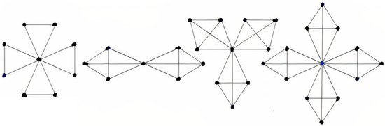
Figure 2. Windmill graphs: $W{d}_4^3,W{d}_2^4,W{d}_3^4,W{d}_4^4,\dots$.

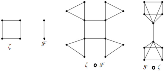
Figure 3. Corona products of $\zeta$ and $\mathcal{F}$.

Definition 1. 

A k-domination regular graph is a type of graph in which every vertex has exactly k neighbors that are also adjacent to each other. In other words, every vertex is adjacent to exactly k vertices that are themselves mutually adjacent.

In this work, the concept of k-domination regular graphs plays a crucial role, and, therefore, it is important to provide a literature review on this terminology. In the following, we provide an overview of the relevant literature on k-domination regular graphs, highlighting their key properties and applications. By understanding the background and context of this concept, readers will be better equipped to comprehend the significance of our research and its contribution to the field. K-domination regular graphs have been studied in several papers in graph theory. For example, in [43], the authors investigate the structure of k-domination regular graphs and show that these graphs have many interesting properties. They also provide several examples of k-domination regular graphs and use them to study the domination number of these graphs. In [44], the authors study the k-domination number of graphs and provide a characterization of k-domination regular graphs. The authors show that a connected graph is k-domination regular if and only if it is regular and satisfies a certain condition related to the k-domination number. They also investigate the relationship between the k-domination number and the total domination number of a graph. In [45], Hansberg et al. investigate some properties of k-domination regular graphs and provide some examples of these graphs. They also study the relationship between the k-domination number and the independence number of a graph, and they show that, for certain families of graphs, the k-domination number and the independence number are equal. Finally, in [46], the authors provide several methods for constructing k-domination regular graphs. They show that k-domination regular graphs can be constructed from other k-domination regular graphs via several operations, including the Cartesian product and composition. They also provide some open problems related to k-domination regular graphs, such as finding the smallest k for which a k-domination regular graph exists. In summary, k-domination regular graphs have been studied extensively in the literature, and they have many interesting properties and applications in graph theory. Further research on these graphs can lead to new insights and solutions in various fields, including computer science, chemistry, and physics.

Our paper aims to address several research questions related to the use of the dominating sigma index in predicting the physicochemical properties of organic compounds. Firstly, we provide an explanation of the dominating sigma index and its relationship with topological indices in mathematical chemistry. Next, we develop linear and non-linear models using the QSPR approach to predict the properties of interest, and we conduct a comparative analysis to evaluate the effectiveness of the domination sigma index and establish an appropriate domination index that correlates with the physicochemical properties of octane and its isomers. Finally, we explore the relationship between topological indices and molecular properties. This paper is structured as follows: Section 3 presents the main results of the domination sigma index, while Section 4 describes the comparative analysis conducted to evaluate its effectiveness and establish an appropriate domination index. Finally, in Section 5, we provide our conclusions and suggestions for further research into QSAR/QSPR domination indices.

3. Main Results

In this section, we give the results of the domination sigma index for the star graph, the complete bipartite and its complement, the book graphs, and the windmill graph.

Proposition 1. 

1. Let $\zeta \simeq S_{r+1}$ be the star graph of $r+1$ vertices; then, $D\sigma \left(S_{r+1}\right)=0.$

2. 

Let $\zeta \simeq K_r$ be the complete graph of r vertices; then, $D\sigma \left(K_r\right)=0.$

3. 

Let $\zeta \simeq S_{r+1,s+1}$ be the double-star graph; then, $D\sigma \left(S_{r+1.s+1}\right)=0.$

4. 

Let $\zeta \simeq K_{r,s}$ be the complete bipartite graph, where $r,s\ge 2$; then, $D\sigma \left(K_{r,s}\right)={\sum }_{uv\in E\left(\zeta \right)}{(s-r)}^2={(s-r)}^{2}rs.$

Proof. 

1. Supposing that $\zeta \simeq S_{r+1}$ is the star graph of r vertices, we have $T_m\left(S_{r+1}\right)=2$ and $d_{p_u}=1$ for all $u\in V\left(S_{r+1}\right).$ Then, $D\sigma \left(S_{r+1}\right)=0.$

2.

Supposing that $\zeta \simeq K_r$ is the complete graph of r vertices, we have $T_m\left(K_r\right)=r$ and $d_{p_u}=1$ for all $u\in V\left(K_r\right).$ Then, $D\sigma \left(K_r\right)=0.$

3.

Supposing that $\zeta \simeq S_{r+1,s+1}$ is the double-star graph, we have $T_m\left(S_{r+1.s+1}\right)=4$ and $d_{p_u}=2$ for all $u\in V\left(S_{r+1.s+1}\right).$ Then, $D\sigma \left(S_{r+1.s+1}\right)=0.$

4.

Supposing that $\zeta \simeq K_{r,s}$ is the complete bipartite graph, where $r,s\ge 2$, we have $T_m\left(K_{r,s}\right)=rs+2$ and

$$d_{p_u}=\left\{\begin{array}{c}r+1\mathrm{if}u\in \mathrm{the}\mathrm{set}\mathrm{of}\mathrm{vertices}\mathrm{that}\mathrm{contains}s\mathrm{vertices}\\ s+1\mathrm{if}u\in \mathrm{the}\mathrm{set}\mathrm{of}\mathrm{vertices}\mathrm{that}\mathrm{contains}r\mathrm{vertices}\end{array}\right.$$

Then,

$$D\sigma \left(K_{r,s}\right)=\sum _{uv\in E\left(\zeta \right)}{(\left(s+1\right)-\left(r+1\right))}^2=\sum _{uv\in E\left(\zeta \right)}{(s-r)}^2={(s-r)}^{2}rs.$$

This completes the proof.

   □

Corollary 1. 

Any graph ζ is a k-domination regular graph if and only if $D\sigma \left(\zeta \right)=0.$

Proof. 

In this case, the sufficient condition is clear. If we consider the necessity condition, $D\sigma \left(\zeta \right)=0,$

$$\begin{array}{cc}\hfill & ⟹\sum _{uv\in E\left(\zeta \right)}{(d_{p_u}-d_{p_v})}^2=0\hfill \\ \hfill & ⟹{(d_{p_u}-d_{p_v})}^2=0\hfill \\ \hfill & ⟹d_{p_u}-d_{p_v}=0\hfill \\ \hfill & ⟹d_{p_u}=d_{p_v}\hfill \end{array}$$

for all $u,v\in V\left(\zeta \right)$, so if $d_{p_u}=d_{p_v}=k$, then $\zeta$ is a k-domination regular graph.   □

Corollary 2. 

Let ζ be the complete bipartite graph $K_{r,s}.$ Then, $D\sigma \left(K_{r,s}\right)=\sigma \left(K_{r,s}\right).$

Proof. 

We have

$$\begin{array}{cc}\hfill D\sigma \left(K_{r,s}\right)& =\sum _{uv\in E\left(\zeta \right)}{(d_{p_u}-d_{p_v})}^2=\sum _{uv\in E\left(K_{r,s}\right)}{(\left(d_u+1\right)-\left(d_v+1\right))}^2\hfill \\ \hfill & =\sum _{uv\in E\left(K_{r,s}\right)}{(d_u-d_v)}^2=\sigma \left(K_{r,s}\right).\hfill \end{array}$$

  □

Proposition 2. 

If $\zeta \simeq K_{r,s},$ then $D\sigma \left(\overline{K_{r,s}}\right)=\overline{\sigma \left(K_{r,s}\right)}$

Proof. 

Since $d_{p_{\overline{K_{r,s}}}}=d_{K_{r,s}},$ we have

$$\begin{array}{cc}\hfill D\sigma \left(\overline{K_{r,s}}\right)& =\sum _{uv\in E\left(\overline{K_{r,s}}\right)}{(d_{p_u}-d_{p_v})}^2\hfill \\ \hfill & =\sum _{uv\notin E\left(K_{r,s}\right)}{(d_u-d_v)}^2=\overline{\sigma \left(K_{r,s}\right)}.\hfill \end{array}$$

  □

Theorem 1. 

If $\zeta \simeq W{d}_r^s$, where $s,r\ge 2$, then $D\sigma \left(W{d}_r^s\right)=s(r-1){(1-{(r-1)}^{s-1})}^2.$

Proof. 

If $\zeta \simeq W{d}_r^s$, where $s,r\ge 2,$ we have $T_m\left(\zeta \right)={\left(r-1\right)}^s+1$ and

$$d_{p_u}=\left\{\begin{array}{c}1\mathrm{if}u\mathrm{is}\mathrm{the}\mathrm{center}\mathrm{vertex},\\ {\left(r-1\right)}^{s-1}\mathrm{otherwise}.\end{array}\right.$$

Suppose

$$\begin{array}{cc}\hfill E_1& =\left\{e:e\in E\left(W{d}_r^s\right),\mathrm{all}\mathrm{edges}\mathrm{that}\mathrm{are}\mathrm{incident}\mathrm{with}\mathrm{the}\mathrm{center}\mathrm{vertex}\right\}.\hfill \\ \hfill E_2& =\left\{e:e\in E\left(W{d}_r^s\right),\mathrm{all}\mathrm{edges}\mathrm{of}\mathrm{the}\mathrm{complete}\mathrm{graph}\right\}.\hfill \end{array}$$

Then, we obtain

$$\begin{array}{cc}\hfill D\sigma \left(W{d}_r^s\right)& =\sum _{uv\in E_1\left(\zeta \right)}{(1-{\left(r-1\right)}^{s-1})}^2+\sum _{uv\in E_2\left(\zeta \right)}{({\left(r-1\right)}^{s-1}-{\left(r-1\right)}^{s-1})}^2\hfill \\ \hfill & ={(1-{\left(r-1\right)}^{s-1})}^2\left|E_1\right|\hfill \\ \hfill & ={(1-{\left(r-1\right)}^{s-1})}^2\left(s\left(r-1\right)\right).\hfill \end{array}$$

This completes the proof.  □

Theorem 2. 

If $\zeta \simeq B_r$ is the book graph for $r\ge 3,$ then $D\sigma \left(B_r\right)=r\left(8-2^{r+2}+2^{2r-1}\right).$

Proof. 

If $\zeta \simeq B_r$ is the book graph for $r\ge 3,$ we have $T_m\left(B_r\right)=2^r+3$ and

$$d_{p_u}=\left\{\begin{array}{c}3\mathrm{if}u\mathrm{is}\mathrm{the}\mathrm{center}\mathrm{vertex},\\ 2^{r-1}+1\mathrm{otherwise}.\end{array}\right.$$

Suppose that $E_1$ denote the set of r edges $u_i{v}_i$ with the initial and terminal vertices of the same domination degree $\left(2^{r-1}+1\right).$ Let $E_2$ denote the set containing only one edge $uv$ with the initial and terminal vertices of the same domination degree 3. Let $E_3$ denote the set of $2r$ edges of the initial vertices of domination degree 3 and the terminal vertices of the domination degree $\left(2^{r-1}+1\right).$ Hence,

$$\begin{array}{cc}\hfill D\sigma \left(B_r\right)& =\sum _{uv\in E_1\left(\zeta \right)}{(\left(\left(2^{r-1}+1\right)\right)-\left(2^{r-1}+1\right))}^2+\hfill \\ \hfill & \sum _{uv\in E_2\left(\zeta \right)}{(3-3)}^2+\sum _{uv\in E_3\left(\zeta \right)}{(3-\left(2^{r-1}+1\right))}^2\hfill \\ \hfill & =2r{\left(2-2^{r-1}\right)}^2=r\left(8-2^{r+2}+2^{2r-1}\right).\hfill \end{array}$$

This completes the proof.   □

Theorem 3. 

If $\zeta \simeq K_{n_1,n_2,\dots ,n_k}$, where $n_1,n_2,\dots ,n_k\ge 2$, then $D\sigma \left(K_{n_1,n_2,\dots ,n_k}\right)=\sigma \left(K_{n_1,n_2,\dots ,n_k}\right).$

Proof. 

Suppose that $\zeta \simeq K_{n_1,n_2,\dots ,n_k}$, where $n_1,n_2,\dots ,n_k\ge 2$. Note that, for any vertex $v\in K_{n_1,n_2,\dots ,n_k}$, we have $d_{p_v}=d_v+1$ and $\left|E\left(K_{n_1,n_2,\dots ,n_k}\right)\right|=T_m\left(K_{n_1,n_2,\dots ,n_k}\right)-k,$ where $T_m\left(K_{n_1,n_2,\dots ,n_k}\right)=\sum _{i=2}^k{n}_2{n}_i+\cdots +n_{k-1}{n}_k+k.$ Hence,

$$\begin{array}{cc}\hfill D\sigma \left(K_{n_1,n_2,\dots ,n_k}\right)& =\sum _{uv\in E\left(\zeta \right)}{\left((d_u+1)-(d_v+1)\right)}^2\hfill \\ \hfill & =\sum _{uv\in E\left(\zeta \right)}{(d_u-d_v)}^2\hfill \\ \hfill & =\sigma \left(K_{n_1,n_2,\dots ,n_k}\right).\hfill \end{array}$$

  □

3.1. Domination Sigma Index of Some Graph Operations

This part provides the domination sigma index values for some graph operations, such as the corona product and the join of graphs. In the following Theorem, we calculate the domination sigma index for the corona graph of any graph $\zeta$ and the complete graph and its complement.

Theorem 4. 

1. For any connected graph ζ of $n_1$ vertices and $m_1$ edges, $D\sigma \left(\zeta \circ k_{n_2}\right)=0.$

2. 

For any connected graph ζ of $n_1$ vertices and $m_1$ edges, $D\sigma \left(\zeta \circ \overline{k_{n_2}}\right)=0.$

Proof. 

(1) Let $\xi \simeq \zeta \circ k_{n_2}.$ We note that there are ${\left(n_2+1\right)}^{n_1}$ minimal dominating sets in $\xi$ and $d_{p_v}={\left(n_2+1\right)}^{n_1-1}.$ Furthermore, there are three types of edges in $\xi .$ All edges of $\zeta ,$ all edges of $k_{n_2},$ and $E_1$ denote the set of all edges that connect a vertex from $\zeta$ and a vertex from $k_{n_2}.$ So, we have

$$\begin{array}{cc}\hfill D\sigma \left(\zeta \circ k_{n_2}\right)& =\sum _{uv\in E\left(\zeta \right)}{(d_{p_u}-d_{p_v})}^2+\sum _{uv\in E\left(k_{n_2}\right)}{(d_{p_u}-d_{p_v})}^2+\sum _{uv\in E_1}{(d_{p_u}-d_{p_v})}^2\hfill \\ \hfill & =\sum _{uv\in E\left(\zeta \right)}{({\left(n_2+1\right)}^{n_1-1}-{\left(n_2+1\right)}^{n_1-1})}^2\hfill \\ \hfill & +\sum _{uv\in E\left(k_{n_2}\right)}{({\left(n_2+1\right)}^{n_1-1}-{\left(n_2+1\right)}^{n_1-1})}^2\hfill \\ \hfill & +\sum _{uv\in E_1}{({\left(n_2+1\right)}^{n_1-1}-{\left(n_2+1\right)}^{n_1-1})}^2=0+0+0=0.\hfill \end{array}$$

(2)

Let $\xi \simeq \zeta \circ \overline{k_{n_2}};$ for any vertex $v\in V\left(\xi \right)$, we have $T_m\left(\xi \right)={\displaystyle \sum _{i=1}^{n_1}}\left(\begin{array}{c}{n}_1\\ i\end{array}\right)$ and $d_{p_v}=T_m\left(\xi \right)-2^{n_1-1}.$ Hence, $\xi$ is a k- domination regular graph, where $k=T_m\left(\xi \right)-2^{n_1-1}$, which implies that $D\sigma \left(\zeta \circ \overline{k_{n_2}}\right)=0.$

  □

In the following Theorems, we calculate the domination sigma index for different cases of the join of two graphs. However, first, we need the following Lemma:

Lemma 1 

([36]). Let ${\zeta }_1$ and ${\zeta }_2$ be any non-complete graphs of $n_1$ and $n_2$ vertices, respectively, and there is no vertex in ${\zeta }_1$ or ${\zeta }_2$ of full degree. Then, $T_m\left({\zeta }_1+{\zeta }_2\right)=T_m\left({\zeta }_1)+T_m({\zeta }_2\right)+n_1{n}_2$ and

$$d_{p_{{\zeta }_1+{\zeta }_2}}\left(v\right)=\left\{\begin{array}{c}{d}_{p_{{\zeta }_1}}\left(v\right)+n_2\mathrm{if}v\in V\left({\zeta }_1\right)\\ d_{p_{{\zeta }_2}}\left(v\right)+n_1\mathrm{if}v\in V\left({\zeta }_2\right).\end{array}\right.$$

Theorem 5. 

Let ${\zeta }_1$ and ${\zeta }_2$ be any non-complete graphs of $n_1$ and $n_2$ vertices, respectively, and there is no vertex in ${\zeta }_1$ or ${\zeta }_2$ of full degree. Then,

$$\begin{array}{cc}\hfill D\sigma \left({\zeta }_1+{\zeta }_2\right)& =D\sigma \left({\zeta }_1)+D\sigma ({\zeta }_2\right)+n_2{\displaystyle \sum _{u\in V\left({\zeta }_1\right)}}{(d_{p_{{\zeta }_1}}\left(u\right)+n_2)}^2\hfill \\ \hfill & +n_1\sum _{v\in V\left({\zeta }_2\right)}{(d_{p_{{\zeta }_2}}\left(v\right)+n_1)}^2-2\rho \left({\zeta }_1\right)\rho \left({\zeta }_2\right)\hfill \\ \hfill & -2n_1{n}_2\rho \left({\zeta }_1\right)-2n_1{n}_2\rho \left({\zeta }_2\right)-2n_1^2{n}_2^2.\hfill \end{array}$$

Proof. 

Let ${\zeta }_1$ and ${\zeta }_2$ be any non-complete graphs of $n_1$ and $n_2$ vertices, respectively, and there is no vertex in ${\zeta }_1$ or ${\zeta }_2$ of full degree. Then,

$$\begin{array}{cc}\hfill D\sigma \left({\zeta }_1+{\zeta }_2\right)& =\stackrel{\left(1\right)}{\overbrace{\sum _{uv\in E\left({\zeta }_1\right)}{(d_{p_{{\zeta }_1+{\zeta }_2}}\left(u\right)-d_{p_{{\zeta }_1+{\zeta }_2}}\left(v\right))}^2}}+\stackrel{\left(2\right)}{\overbrace{\sum _{uv\in E\left({\zeta }_2\right)}{(d_{p_{{\zeta }_1+{\zeta }_2}}\left(u\right)-d_{p_{{\zeta }_1+{\zeta }_2}}\left(v\right))}^2}}\hfill \\ \hfill & +\stackrel{\left(3\right)}{\overbrace{\sum _{\begin{array}{c}u\in V\left({\zeta }_1\right)\\ v\in V\left({\zeta }_2\right)\end{array}}{(d_{p_{{\zeta }_1+{\zeta }_2}}\left(u\right)-d_{p_{{\zeta }_1+{\zeta }_2}}\left(v\right))}^2}}\hfill \end{array}$$

For (1):

$$\begin{array}{cc}\hfill \sum _{uv\in E({\zeta }_1)}{(d_{p_{{\zeta }_1+{\zeta }_2}}\left(u\right)-d_{p_{{\zeta }_1+{\zeta }_2}}\left(v\right))}^2& =\sum _{uv\in E({\zeta }_1)}(d_{p_{{\zeta }_1}}\left(u\right)+n_2)-(d_{p_{{\zeta }_1}}\left(v\right)+n_2){)}^2\hfill \\ \hfill & =\sum _{uv\in E\left({\zeta }_1\right)}{(d_{p_{{\zeta }_1}}\left(u\right)-d_{p_{{\zeta }_1}}\left(v\right))}^2=D\sigma \left({\zeta }_1\right)\hfill \end{array}$$

For (2):

$$\begin{array}{cc}\hfill \sum _{uv\in E\left({\zeta }_2\right)}{(d_{p_{{\zeta }_1+{\zeta }_2}}\left(u\right)-d_{p_{{\zeta }_1+{\zeta }_2}}\left(v\right))}^2& =\sum _{uv\in E\left({\zeta }_2\right)}(d_{p_{{\zeta }_2}}\left(u\right)+n_1)-(d_{p_{{\zeta }_2}}\left(v\right)+n_1){)}^2\hfill \\ \hfill & =\sum _{uv\in E({\zeta }_2)}{(d_{p_{{\zeta }_2}}\left(u\right)-d_{p_{{\zeta }_2}}\left(v\right))}^2=D\sigma \left({\zeta }_2\right)\hfill \end{array}$$

For (3):

$$\begin{array}{cc}\hfill & \sum _{{}_{\begin{array}{c}u\in V\left({\zeta }_1\right)\\ v\in V\left({\zeta }_2\right)\end{array}}}{(d_{p_{{\zeta }_1+{\zeta }_2}}\left(u\right)-d_{p_{{\zeta }_1+{\zeta }_2}}\left(v\right))}^2\hfill \\ \hfill & ={\left[\left(d_{p_{{\zeta }_1}}\left(u_1\right)+n_2\right)-\left(d_{p_{{\zeta }_2}}\left(v_1\right)+n_1\right)\right]}^2+\hfill \\ \hfill & {\left[\left(d_{p_{{\zeta }_1}}\left(u_1\right)+n_2\right)-\left(d_{p_{{\zeta }_2}}\left(v_2\right)+n_1\right)\right]}^2+\cdots +\hfill \\ \hfill & {\left[\left(d_{p_{{\zeta }_1}}\left(u_1\right)+n_2\right)-\left(d_{p_{{\zeta }_2}}\left(v_{n_2}\right)+n_1\right)\right]}^2+\hfill \\ \hfill & {\left[\left(d_{p_{{\zeta }_1}}\left(u_2\right)+n_2\right)-\left(d_{p_{{\zeta }_2}}\left(v_1\right)+n_1\right)\right]}^2+\hfill \\ \hfill & {\left[\left(d_{p_{{\zeta }_1}}\left(u_2\right)+n_2\right)-\left(d_{p_{{\zeta }_2}}\left(v_2\right)+n_1\right)\right]}^2+\cdots +\hfill \\ \hfill & {\left[\left(d_{p_{{\zeta }_1}}\left(u_2\right)+n_2\right)-\left(d_{p_{{\zeta }_2}}\left(v_{n_2}\right)+n_1\right)\right]}^2+\cdots +\hfill \\ \hfill & {\left[\left(d_{p_{{\zeta }_1}}\left(u_{n_1}\right)+n_2\right)-\left(d_{p_{{\zeta }_2}}\left(v_1\right)+n_1\right)\right]}^2+\hfill \\ \hfill & {\left[\left(d_{p_{{\zeta }_1}}\left(u_{n_1}\right)+n_2\right)-\left(d_{p_{{\zeta }_2}}\left(v_2\right)+n_1\right)\right]}^2+\cdots +\hfill \\ \hfill & {\left[\left(d_{p_{{\zeta }_1}}\left(u_{n_1}\right)+n_2\right)-\left(d_{p_{{\zeta }_2}}\left(v_{n_2}\right)+n_1\right)\right]}^2\hfill \\ \hfill & =n_2{\left(d_{p_{{\zeta }_1}}\left(u_1\right)+n_2\right)}^2+\sum _{v\in V\left({\zeta }_2\right)}{\left(d_{p_{{\zeta }_2}}\left(v\right)+n_1\right)}^2-\hfill \\ \hfill & 2d_{p_{{\zeta }_1}}\left(u_1\right)\sum _{v\in V\left({\zeta }_2\right)}{d}_{p_{{\zeta }_2}}\left(v\right)-2n_1{n}_2{d}_{p_{{\zeta }_1}}\left(u_1\right)-\hfill \\ \hfill & 2n_2\sum _{v\in V\left({\zeta }_2\right)}{d}_{p_{{\zeta }_2}}\left(v\right)-2n_1{n}_2^2+n_2{\left(d_{p_{{\zeta }_1}}\left(u_2\right)+n_2\right)}^2+\hfill \\ \hfill & \sum _{v\in V\left({\zeta }_2\right)}{\left(d_{p_{{\zeta }_2}}\left(v\right)+n_1\right)}^2-\hfill \\ \hfill & 2d_{p_{{\zeta }_1}}\left(u_2\right)\sum _{v\in V\left({\zeta }_2\right)}{d}_{p_{{\zeta }_2}}\left(v\right)-2n_1{n}_2{d}_{p_{{\zeta }_1}}\left(u_2\right)-\hfill \\ \hfill & 2n_1{n}_2{d}_{p_{{\zeta }_1}}\left(u_2\right)-2n_2\sum _{v\in V\left({\zeta }_2\right)}{d}_{p_{{\zeta }_2}}\left(v\right)-2n_1{n}_2^2+\cdots +\hfill \\ \hfill & n_2{\left(d_{p_{{\zeta }_1}}\left(u_{n_1}\right)+n_2\right)}^2+\sum _{v\in V\left({\zeta }_2\right)}{\left(d_{p_{{\zeta }_2}}\left(v\right)+n_1\right)}^2\hfill \\ \hfill & -2d_{p_{{\zeta }_1}}\left(u_{n_1}\right)\sum _{v\in V\left({\zeta }_2\right)}{d}_{p_{{\zeta }_2}}\left(v\right)-2n_1{n}_2{d}_{p_{\zeta }}\left(u_{n_1}\right)-\hfill \\ \hfill & 2n_2\sum _{v\in V\left({\zeta }_2\right)}{d}_{p_{{\zeta }_2}}\left(v\right)-2n_1{n}_2^2\hfill \\ \hfill & =n_2\sum _{u\in V\left({\zeta }_1\right)}{\left(d_{p_{{\zeta }_1}}\left(u\right)+n_2\right)}^2+n_1\sum _{v\in V\left({\zeta }_2\right)}{\left(d_{p_{{\zeta }_2}}\left(v\right)+n_1\right)}^2\hfill \\ \hfill & -2\sum _{u\in V\left({\zeta }_1\right)}{d}_{p_{{\zeta }_1}}\left(u\right)\sum _{v\in V\left({\zeta }_2\right)}{d}_{p_{{\zeta }_2}}\left(v\right)-\hfill \\ \hfill & 2n_1{n}_2\sum _{u\in V\left({\zeta }_1\right)}{d}_{p_{{\zeta }_1}}\left(u\right)-2n_1{n}_2\sum _{v\in V\left({\zeta }_2\right)}{d}_{p_{{\zeta }_2}}\left(v\right)-2n_1^2{n}_2^2\hfill \\ \hfill & =n_2\sum _{u\in V\left({\zeta }_1\right)}{\left(d_{p_{{\zeta }_1}}\left(u\right)+n_2\right)}^2+n_1\sum _{v\in V\left({\zeta }_2\right)}{\left(d_{p_{{\zeta }_2}}\left(v\right)+n_1\right)}^2-2\rho \left({\zeta }_1\right)\rho \left({\zeta }_2\right)-2n_1{n}_2\rho \left({\zeta }_1\right)-\hfill \\ \hfill & 2n_1{n}_2\rho \left({\zeta }_2\right)-2n_1^2{n}_2^2.\hfill \end{array}$$

Now, by adding (1), (2), and (3), we conclude our result.   □

Using the fact [36] that, for any graph $\zeta ,$ we have $\rho$$\left(\zeta \right)\le T_m\left({\zeta }_1\right)\mathsf{\Gamma }\left(\zeta \right),$ we conclude the following:

Corollary 3. 

Let ${\zeta }_1$ and ${\zeta }_2$ be any non-complete graphs of $n_1$ and $n_2$ vertices, respectively, and there is no vertex in ${\zeta }_1$ or ${\zeta }_2$ of full degree. Then,

$$\begin{array}{cc}\hfill D\sigma \left({\zeta }_1+{\zeta }_2\right)& \le D\sigma \left({\zeta }_1)+D\sigma ({\zeta }_2\right)+n_2\sum _{u\in V\left({\zeta }_1\right)}{(d_{p_{{\zeta }_1}}\left(u\right)-n_2)}^2+n_1\sum _{v\in V\left({\zeta }_2\right)}{(d_{p_{{\zeta }_2}}\left(v\right)-n_1)}^2-\hfill \\ \hfill & 2T_m\left({\zeta }_1\right)\mathsf{\Gamma }\left({\zeta }_1\right)T_m\left({\zeta }_2\right)\mathsf{\Gamma }\left({\zeta }_2\right)-2n_1{n}_2{T}_m\left({\zeta }_1\right)\mathsf{\Gamma }\left({\zeta }_1\right)-2n_1{n}_2{T}_m\left({\zeta }_2\right)\mathsf{\Gamma }\left({\zeta }_2\right)-2n_1^2{n}_2^2.\hfill \end{array}$$

Proposition 3. 

Let ${\zeta }_1$ and ${\zeta }_2$ both be complete graphs of $n_1$ and $n_2$ vertices, respectively. Then, $D\sigma \left({\zeta }_1+{\zeta }_2\right)=0.$

Proof. 

Let ${\zeta }_1$ and ${\zeta }_2$ both be complete graphs of $n_1$ and $n_2$ vertices, respectively; then, $T_m\left({\zeta }_1+{\zeta }_2\right)=n_1+n_2$ and $d_{p_{{\zeta }_1+{\zeta }_2}}\left(v\right)=1$ for all $v\in V\left({\zeta }_1+{\zeta }_2\right)$, which implies that ${\zeta }_1+{\zeta }_2$ is a 1-domination regular graph. Hence, $D\sigma \left({\zeta }_1+{\zeta }_2\right)=0.$   □

Theorem 6. 

If ${\zeta }_1$ is a complete graph and ${\zeta }_2$ is not a complete graph of $n_1$ and $n_2$ vertices, respectively, then

$$D\sigma \left({\zeta }_1+{\zeta }_2\right)=D\sigma \left({\zeta }_2\right)+n_1{n}_2+n_{1}D{M}_1\left({\zeta }_2\right)-2n_1\rho \left({\zeta }_2\right).$$

Proof. 

Let ${\zeta }_1$ be a complete graph and ${\zeta }_2$ not be a complete graph of $n_1$ and $n_2$ vertices, respectively; then, $T_m\left({\zeta }_1+{\zeta }_2\right)=n_1+T_m\left({\zeta }_2\right)$ and

$$d_{p_{{\zeta }_1+{\zeta }_2}}\left(v\right)=\left\{\begin{array}{c}1\mathrm{if}v\in V\left({\zeta }_1\right)\\ d_{p_{{\zeta }_2}}\left(v\right)\mathrm{if}v\in V\left({\zeta }_2\right).\end{array}\right.$$

Hence,

$$\begin{array}{cc}\hfill D\sigma \left({\zeta }_1+{\zeta }_2\right)& =\stackrel{\left(1\right)}{\overbrace{\sum _{uv\in E\left({\zeta }_1\right)}{(d_{p_{{\zeta }_1+{\zeta }_2}}\left(u\right)-d_{p_{{\zeta }_1+{\zeta }_2}}\left(v\right))}^2}}+\hfill \\ \hfill & \stackrel{\left(2\right)}{\overbrace{\sum _{uv\in E\left({\zeta }_2\right)}{(d_{p_{{\zeta }_1+{\zeta }_2}}\left(u\right)-d_{p_{{\zeta }_1+{\zeta }_2}}\left(v\right))}^2}}+\hfill \\ \hfill & \stackrel{\left(3\right)}{\overbrace{\sum _{\begin{array}{c}u\in V\left({\zeta }_1\right)\\ v\in V\left({\zeta }_2\right)\end{array}}{(d_{p_{{\zeta }_1+{\zeta }_2}}\left(u\right)-d_{p_{{\zeta }_1+{\zeta }_2}}\left(v\right))}^2}}\hfill \end{array}$$

For (1):

$$\sum _{uv\in E\left({\zeta }_1\right)}{(d_{p_{{\zeta }_1+{\zeta }_2}}\left(u\right)-d_{p_{{\zeta }_1+{\zeta }_2}}\left(v\right))}^2=\sum _{uv\in E\left({\zeta }_1\right)}{(1-1)}^2=0.$$

For (2):

$$\sum _{uv\in E\left({\zeta }_2\right)}{(d_{p_{{\zeta }_1+{\zeta }_2}}\left(u\right)-d_{p_{{\zeta }_1+{\zeta }_2}}\left(v\right))}^2=\sum _{uv\in E\left({\zeta }_2\right)}{(d_{p_{{\zeta }_2}}\left(u\right)-d_{p_{{\zeta }_2}}\left(v\right))}^2=D\sigma \left({\zeta }_2\right).$$

For (3):

$$\begin{array}{cc}\hfill \sum _{\begin{array}{c}u\in V\left({\zeta }_1\right)\\ v\in V\left({\zeta }_2\right)\end{array}}{(d_{p_{{\zeta }_1+{\zeta }_2}}\left(u\right)-d_{p_{{\zeta }_1+{\zeta }_2}}\left(v\right))}^2& ={\left(1-d_{p_{{\zeta }_2}}\left(v_1\right)\right)}^2+{\left(1-d_{p_{{\zeta }_2}}\left(v_2\right)\right)}^2\hfill \\ \hfill & +\cdots +{\left(1-d_{p_{{\zeta }_2}}\left(v_{n_2}\right)\right)}^2+\hfill \\ \hfill & {\left(1-d_{p_{{\zeta }_2}}\left(v_1\right)\right)}^2+{\left(1-d_{p_{{\zeta }_2}}\left(v_2\right)\right)}^2\hfill \\ \hfill & +\cdots +{\left(1-d_{p_{{\zeta }_2}}\left(v_{n_2}\right)\right)}^2+\cdots +\hfill \\ \hfill & {\left(1-d_{p_{{\zeta }_2}}\left(v_1\right)\right)}^2+{\left(1-d_{p_{{\zeta }_2}}\left(v_2\right)\right)}^2\hfill \\ \hfill & +\cdots +{\left(1-d_{p_{{\zeta }_2}}\left(v_{n_2}\right)\right)}^2\hfill \\ \hfill & =(1+d_{p_{{\zeta }_2}}^2\left(v_1\right)-2d_{p_{{\zeta }_2}}\left(v_1\right))+\hfill \\ \hfill & (1+d_{p_{{\zeta }_2}}^2\left(v_2\right)-2d_{p_{{\zeta }_2}}\left(v_2\right))+\cdots +\hfill \\ \hfill & (1+d_{p_{{\zeta }_2}}^2\left(v_{n_2}\right)-2d_{p_{{\zeta }_2}}\left(v_{n_2}\right))+\hfill \\ \hfill & (1+d_{p_{{\zeta }_2}}^2\left(v_1\right)-2d_{p_{{\zeta }_2}}\left(v_1\right))+\hfill \\ \hfill & (1+d_{p_{{\zeta }_2}}^2\left(v_2\right)-2d_{p_{{\zeta }_2}}\left(v_2\right))+\cdots +\hfill \\ \hfill & (1+d_{p_{{\zeta }_2}}^2\left(v_{n_2}\right)-2d_{p_{{\zeta }_2}}\left(v_{n_2}\right))+\cdots +\hfill \\ \hfill & (1+d_{p_{{\zeta }_2}}^2\left(v_1\right)-2d_{p_{{\zeta }_2}}\left(v_1\right))+\hfill \\ \hfill & (1+d_{p_{{\zeta }_2}}^2\left(v_2\right)-2d_{p_{{\zeta }_2}}\left(v_2\right))+\cdots +\hfill \\ \hfill & (1+d_{p_{{\zeta }_2}}^2\left(v_{n_2}\right)-2d_{p_{{\zeta }_2}}\left(v_{n_2}\right))\hfill \\ \hfill & =\left(n_2+\sum _{v\in V\left({\zeta }_2\right)}{d}_{p_{{\zeta }_2}}^2\left(v\right)-2\sum _{v\in V\left({\zeta }_2\right)}{d}_{p_{{\zeta }_2}}\left(v\right)\right)+\hfill \\ \hfill & \left(n_2+\sum _{v\in V\left({\zeta }_2\right)}{d}_{p_{{\zeta }_2}}^2\left(v\right)-2\sum _{v\in V\left({\zeta }_2\right)}{d}_{p_{{\zeta }_2}}\left(v\right)\right)+\cdots +\hfill \\ \hfill & \left(n_2+\sum _{v\in V\left({\zeta }_2\right)}{d}_{p_{{\zeta }_2}}^2\left(v\right)-2\sum _{v\in V\left({\zeta }_2\right)}{d}_{p_{{\zeta }_2}}\left(v\right)\right)\hfill \\ \hfill & =n_1{n}_2+n_1\sum _{v\in V\left({\zeta }_2\right)}{d}_{p_{{\zeta }_2}}^2\left(v\right)-2n_1\sum _{v\in V\left({\zeta }_2\right)}{d}_{p_{{\zeta }_2}}\left(v\right)\hfill \\ \hfill & =n_1{n}_2+n_{1}DM\left({\zeta }_2\right)-2n_1\rho \left({\zeta }_2\right).\hfill \end{array}$$

By adding $\left(1\right),\left(2\right)$, and $\left(3\right)$, we complete the proof.   □

Theorem 7. 

If ${\zeta }_1$ is not a complete graph and ${\zeta }_2$ is a complete graph of $n_1$ and $n_2$ vertices, respectively, then

$$D\sigma \left({\zeta }_1+{\zeta }_2\right)=D\sigma \left({\zeta }_1\right)+n_1{n}_2+n_{2}D{M}_1\left({\zeta }_1\right)-2n_1\rho \left({\zeta }_1\right).$$

Proof. 

Let ${\zeta }_1$ not be a complete graph and ${\zeta }_2$ be a complete graph of $n_1$ and $n_2$ vertices, respectively; then, $T_m\left({\zeta }_1+{\zeta }_2\right)=n_2+T_m\left({\zeta }_1\right)$ and

$$d_{p_{{\zeta }_1+{\zeta }_2}}\left(v\right)=\left\{\begin{array}{c}1\mathrm{if}v\in V\left({\zeta }_2\right)\\ d_{p_{{\zeta }_1}}\left(v\right)\mathrm{if}v\in V\left({\zeta }_1\right).\end{array}\right.$$

Hence,

$$\begin{array}{cc}\hfill D\sigma \left({\zeta }_1+{\zeta }_2\right)& =\stackrel{\left(1\right)}{\overbrace{\sum _{uv\in E\left({\zeta }_1\right)}{(d_{p_{{\zeta }_1+{\zeta }_2}}\left(u\right)-d_{p_{{\zeta }_1+{\zeta }_2}}\left(v\right))}^2}}+\stackrel{\left(2\right)}{\overbrace{\sum _{uv\in E\left({\zeta }_2\right)}{(d_{p_{{\zeta }_1+{\zeta }_2}}\left(u\right)-d_{p_{{\zeta }_1+{\zeta }_2}}\left(v\right))}^2}}+\hfill \\ \hfill & \stackrel{\left(3\right)}{\overbrace{\sum _{\begin{array}{c}u\in V\left({\zeta }_1\right)\\ v\in V\left({\zeta }_2\right)\end{array}}{(d_{p_{{\zeta }_1+{\zeta }_2}}\left(u\right)-d_{p_{{\zeta }_1+{\zeta }_2}}\left(v\right))}^2}}\hfill \end{array}$$

For (1):

$$\sum _{uv\in E\left({\zeta }_1\right)}{(d_{p_{{\zeta }_1+{\zeta }_2}}\left(u\right)-d_{p_{{\zeta }_1+{\zeta }_2}}\left(v\right))}^2=\sum _{uv\in E\left({\zeta }_2\right)}{(d_{p_{{\zeta }_1}}\left(u\right)-d_{p_{{\zeta }_1}}\left(v\right))}^2=D\sigma \left({\zeta }_1\right).$$

For (2):

$$\sum _{uv\in E\left({\zeta }_2\right)}{(d_{p_{{\zeta }_1+{\zeta }_2}}\left(u\right)-d_{p_{{\zeta }_1+{\zeta }_2}}\left(v\right))}^2=\sum _{uv\in E\left({\zeta }_2\right)}{(1-1)}^2=0.$$

For (3):

$$\begin{array}{cc}\hfill \sum _{\begin{array}{c}u\in V\left({\zeta }_1\right)\\ v\in V\left({\zeta }_2\right)\end{array}}{(d_{p_{{\zeta }_1+{\zeta }_2}}\left(u\right)-d_{p_{{\zeta }_1+{\zeta }_2}}\left(v\right))}^2& ={\left(d_{p_{{\zeta }_1}}\left(u_1\right)-1\right)}^2+{\left(d_{p_{{\zeta }_1}}\left(u_1\right)-1\right)}^2\hfill \\ \hfill & +\cdots +{\left(d_{p_{{\zeta }_1}}\left(v_1\right)-1\right)}^2+\hfill \\ \hfill & {\left(d_{p_{{\zeta }_1}}\left(u_2\right)-1\right)}^2+{\left(d_{p_{{\zeta }_1}}\left(u_2\right)-1\right)}^2+\dots \hfill \\ \hfill & +{\left(d_{p_{{\zeta }_1}}\left(v_{n_2}\right)-1\right)}^2+\cdots +\hfill \\ \hfill & {\left(d_{p_{{\zeta }_1}}\left(u_{n_1}\right)-1\right)}^2+{\left(d_{p_{{\zeta }_1}}\left(u_{n_1}\right)-1\right)}^2\hfill \\ \hfill & +\cdots +{\left(d_{p_{{\zeta }_1}}\left(u_{n_1}\right)-1\right)}^2\hfill \\ \hfill & =n_2{\left(d_{p_{{\zeta }_1}}\left(u_1\right)-1\right)}^2+n_2{\left(d_{p_{{\zeta }_1}}\left(u_2\right)-1\right)}^2\hfill \\ \hfill & +\cdots +n_2{\left(d_{p_{{\zeta }_1}}\left(u_{n_1}\right)-1\right)}^2\hfill \\ \hfill & =n_2\sum _{u\in V\left({\zeta }_1\right)}{\left(d_{p_{{\zeta }_1}}\left(u\right)-1\right)}^2\hfill \\ \hfill & =n_2\sum _{u\in V\left({\zeta }_1\right)}\left(d_{p_{{\zeta }_1}}^2\left(u\right)-2d_{p_{{\zeta }_1}}\left(u\right)+1\right)\hfill \\ \hfill & =n_2\sum _{u\in V\left({\zeta }_1\right)}{d}_{p_{{\zeta }_1}}^2\left(u\right)-2n_2\sum _{u\in V\left({\zeta }_1\right)}{d}_{p_{{\zeta }_1}}\left(u\right)+\sum _{u\in V\left({\zeta }_1\right)}1\hfill \\ \hfill & =n_2{n}_1+n_{2}DM\left({\zeta }_1\right)-2n_1\rho \left({\zeta }_1\right).\hfill \end{array}$$

By adding $\left(1\right),\left(2\right)$, and $\left(3\right)$, we complete the proof.   □

Lemma 2. 

If ${\zeta }_1$ and ${\zeta }_2$ are any non-complete graphs of $\left(n_1,m_1\right)$ and $\left(n_2,m_2\right)$ vertices and edges, respectively, such that $A\subseteq {\zeta }_1$ contains all vertices of full degrees and $B\subseteq {\zeta }_2$ contains all vertices of full degrees, then $T_m\left({\zeta }_1+{\zeta }_2\right)=T_m\left({\zeta }_1\right)+T_m\left({\zeta }_2\right)+\left(n_1-A\right)\left(n_2-B\right)$ and

$$d_{p_{{\zeta }_1+{\zeta }_2}}\left(v\right)=\left\{\begin{array}{c}{d}_{p_{{\zeta }_1}}\left(v\right)+\left(n_2-\left|B\right|\right)\mathrm{if}v\in V\left({\zeta }_1\right)\mathrm{and}v\notin A,\\ d_{p_{{\zeta }_2}}\left(v\right)\left(n_1-\left|A\right|\right)\mathrm{if}v\in V\left({\zeta }_2\right)\mathrm{and}v\notin B,\\ d_{p_{{\zeta }_1}}\left(v\right)\mathrm{if}v\in V\left({\zeta }_1\right)\mathrm{and}v\in A,\\ d_{p_{{\zeta }_2}}\left(v\right)\mathrm{if}v\in V\left({\zeta }_2\right)\mathrm{and}v\in B.\end{array}\right.$$

Theorem 8. 

If ${\zeta }_1$ and ${\zeta }_2$ are any non-complete graphs of $\left(n_1,m_1\right)$ and $\left(n_2,m_2\right)$ vertices and edges, respectively, such that $A\subseteq V\left({\zeta }_1\right)$ contains all vertices of full degrees and $B\subseteq V\left({\zeta }_2\right)$ contains all vertices of full degrees, then

$$\begin{array}{ccc}\hfill D\sigma \left({\zeta }_1+{\zeta }_2\right)& =& D\sigma \left({\zeta }_1\right)+D\sigma \left({\zeta }_2\right)+{\left(n_2-\left|B\right|\right)}^2\left|E_5\right|+{\left(n_1-\left|A\right|\right)}^2\left|E_6\right|-\hfill \\ & & 2\left[\begin{array}{c}\left(n_2-\left|B\right|\right)\sum _{\begin{array}{c}uv\in E_5\\ u\notin A\\ v\in A\end{array}}\left(d_{p_{{\zeta }_1}}\left(u\right)-d_{p_{{\zeta }_1}}\left(v\right)\right)+\\ \left(n_1-\left|A\right|\right)\sum _{\begin{array}{c}uv\in E_6\\ u\notin B\\ v\in B\end{array}}\left(d_{p_{{\zeta }_2}}\left(u\right)-d_{p_{{\zeta }_2}}\left(v\right)\right)\end{array}\right]+\hfill \\ & & \sum _{\begin{array}{c}uv\in E_8\\ u\in V\left({\zeta }_1\right),u\in A\\ v\in V\left({\zeta }_2\right),v\notin B\end{array}}{\left(d_{p_{{\zeta }_1}}\left(u\right)-d_{p_{{\zeta }_2}}\left(v\right)\right)}^2+{\left(n_1-\left|A\right|\right)}^2\left|E_8\right|-\hfill \\ & & 2\left(n_1-\left|A\right|\right)\sum _{\begin{array}{c}uv\in E_8\\ u\in V\left({\zeta }_1\right),u\in A\\ v\in V\left({\zeta }_2\right),v\notin B\end{array}}\left(d_{p_{{\zeta }_1}}\left(u\right)-d_{p_{{\zeta }_2}}\left(v\right)\right)+\hfill \\ & & \sum _{\begin{array}{c}uv\in E_9\\ u\in V\left({\zeta }_1\right),u\notin A\\ v\in V\left({\zeta }_2\right),v\in B\end{array}}{\left(d_{p_{{\zeta }_1}}\left(u\right)-d_{p_{{\zeta }_2}}\left(v\right)\right)}^2+{\left(n_2-\left|B\right|\right)}^2\left|E_9\right|+\hfill \\ & & 2\left(n_2-\left|B\right|\right)\sum _{\begin{array}{c}uv\in E_9\\ u\in V\left({\zeta }_1\right),u\notin A\\ v\in V\left({\zeta }_2\right),v\in B\end{array}}\left(d_{p_{{\zeta }_1}}\left(u\right)-d_{p_{{\zeta }_2}}\left(v\right)\right)+\hfill \\ & & \sum _{\begin{array}{c}uv\in E_{10}\\ u\in V\left({\zeta }_1\right),u\notin A\\ v\in V\left({\zeta }_2\right),v\notin B\end{array}}{\left(d_{p_{{\zeta }_1}}\left(u\right)-d_{p_{{\zeta }_2}}\left(v\right)\right)}^2+{\left(n_2-n_1+\left|A\right|-\left|B\right|\right)}^2\left|E_{10}\right|+\hfill \\ & & 2\left(n_2-n_1+\left|A\right|-\left|B\right|\right)\sum _{\begin{array}{c}uv\in E_{10}\\ u\in V\left({\zeta }_1\right),u\notin A\\ v\in V\left({\zeta }_2\right),v\notin B\end{array}}\left(d_{p_{{\zeta }_1}}\left(u\right)-d_{p_{{\zeta }_2}}\left(v\right)\right).\hfill \end{array}$$

Proof. 

Suppose that ${\zeta }_1$ and ${\zeta }_2$ are any non-complete graphs of $\left(n_1,m_1\right)$ and $\left(n_2,m_2\right)$ vertices and edges, respectively, such that $A\subseteq V\left({\zeta }_1\right)$ contains all vertices of full degrees and $B\subseteq V\left({\zeta }_2\right)$ contains all vertices of full degrees. Then, $T_m\left({\zeta }_1+{\zeta }_2\right)=T_m\left({\zeta }_1\right)+T_m\left({\zeta }_2\right)+\left(n_1-A\right)\left(n_2-B\right)$ and

$$d_{p_{{\zeta }_1+{\zeta }_2}}\left(v\right)=\left\{\begin{array}{c}{d}_{p_{{\zeta }_1}}\left(v\right)+\left(n_2-\left|B\right|\right)\mathrm{if}v\in V\left({\zeta }_1\right)\mathrm{and}v\notin A,\\ d_{p_{{\zeta }_1}}\left(v\right)\mathrm{if}v\in V\left({\zeta }_1\right)\mathrm{and}v\in A,\\ d_{p_{{\zeta }_2}}\left(v\right)+\left(n_1-\left|A\right|\right)\mathrm{if}v\in V\left({\zeta }_2\right)\mathrm{and}v\notin B,\\ d_{p_{{\zeta }_2}}\left(v\right)\mathrm{if}v\in V\left({\zeta }_2\right)\mathrm{and}v\in B.\end{array}\right.$$

We divide the edge set of $\left({\zeta }_1+{\zeta }_2\right)$ according to the degree domination of the vertices as follows:

$$\begin{array}{cc}\hfill E_1& =\{e=uv:u,v\in A\},E_2=\{e=uv:u,v\in B\},\hfill \\ \hfill E_3& =\{e=uv:u,v\notin A\},E_4=\{e=uv:u,v\notin B\},\hfill \\ \hfill E_5& =\{e=uv:u\in A,v\in \left({\zeta }_1-A\right)\},E_6=\{e=uv:u\in B,v\in \left({\zeta }_2-B\right)\},\hfill \\ \hfill E_7& =\{e=uv:u\in A,v\in B\},E_8=\{e=uv:u\in A,v\in \left({\zeta }_2-B\right)\},\hfill \\ \hfill E_9& =\{e=uv:u\in \left({\zeta }_1-A\right),v\in B\},E_{10}=\{e=uv:u\in \left({\zeta }_1-A\right),v\in \left({\zeta }_2-B\right)\}.\hfill \end{array}$$

Hence,

$$\begin{array}{cc}\hfill D\sigma \left({\zeta }_1+{\zeta }_2\right)& =\stackrel{\left(1\right)}{\overbrace{{\sum }_{uv\in E\left({\zeta }_1\right)}{(d_{p_{{\zeta }_1+{\zeta }_2}}\left(u\right)-d_{p_{{\zeta }_1+{\zeta }_2}}\left(v\right))}^2}}+\hfill \\ \hfill & \stackrel{\left(2\right)}{\overbrace{{\sum }_{uv\in E\left({\zeta }_2\right)}{(d_{p_{{\zeta }_1+{\zeta }_2}}\left(u\right)-d_{p_{{\zeta }_1+{\zeta }_2}}\left(v\right))}^2}}+\hfill \\ \hfill & \stackrel{\left(3\right)}{\overbrace{{\sum }_{\begin{array}{c}u\in V\left({\zeta }_1\right)\\ v\in V\left({\zeta }_2\right)\end{array}}{(d_{p_{{\zeta }_1+{\zeta }_2}}\left(u\right)-d_{p_{{\zeta }_1+{\zeta }_2}}\left(v\right))}^2}}\hfill \\ \hfill & =\sum _{uv\in E_1}{(d_{p_{{\zeta }_1+{\zeta }_2}}\left(u\right)-d_{p_{{\zeta }_1+{\zeta }_2}}\left(v\right))}^2+\cdots +\sum _{uv\in E_{10}}{(d_{p_{{\zeta }_1+{\zeta }_2}}\left(u\right)-d_{p_{{\zeta }_1+{\zeta }_2}}\left(v\right))}^2.\hfill \end{array}$$

Now, we calculate the summation for each term as follows:

$$\begin{array}{cc}\hfill \sum _{uv\in E_1}{(d_{p_{{\zeta }_1+{\zeta }_2}}\left(u\right)-d_{p_{{\zeta }_1+{\zeta }_2}}\left(v\right))}^2& =\sum _{uv\in E_1}{\left(1-1\right)}^2=0\hfill \\ \hfill \sum _{uv\in E_2}{(d_{p_{{\zeta }_1+{\zeta }_2}}\left(u\right)-d_{p_{{\zeta }_1+{\zeta }_2}}\left(v\right))}^2& =\sum _{uv\in E_2}{\left(1-1\right)}^2=0\hfill \\ \hfill \sum _{uv\in E_3}{(d_{p_{{\zeta }_1+{\zeta }_2}}\left(u\right)-d_{p_{{\zeta }_1+{\zeta }_2}}\left(v\right))}^2& =\sum _{uv\in E_3}{\left[\left(d_{p_{{\zeta }_1}}\left(u\right)+\left(n_2-\left|B\right|\right)\right)-\left(d_{p_{{\zeta }_1}}\left(v\right)+\left(n_2-\left|B\right|\right)\right)\right]}^2\hfill \\ \hfill & =\sum _{uv\in E_3}{(d_{p_{{\zeta }_1}}\left(u\right)-d_{p_{{\zeta }_1}}\left(v\right))}^2\hfill \\ \hfill \sum _{uv\in E_4}{(d_{p_{{\zeta }_1+{\zeta }_2}}\left(u\right)-d_{p_{{\zeta }_1+{\zeta }_2}}\left(v\right))}^2& =\sum _{uv\in E_4}{\left[\left(d_{p_{{\zeta }_2}}\left(u\right)+\left(n_1-\left|A\right|\right)\right)-\left(d_{p_{{\zeta }_2}}\left(v\right)+\left(n_1-\left|A\right|\right)\right)\right]}^2\hfill \\ \hfill & =\sum _{uv\in E_4}{(d_{p_{{\zeta }_2}}\left(u\right)-d_{p_{{\zeta }_2}}\left(v\right))}^2\hfill \\ \hfill \sum _{\begin{array}{c}uv\in E_5\\ u\notin A\\ v\in A\end{array}}{(d_{p_{{\zeta }_1+{\zeta }_2}}\left(u\right)-d_{p_{{\zeta }_1+{\zeta }_2}}\left(v\right))}^2& =\sum _{\begin{array}{c}uv\in E_5\\ u\notin A\\ v\in A\end{array}}{\left[\left(d_{p_{{\zeta }_1}}\left(u\right)+\left(n_2-\left|B\right|\right)\right)-d_{p_{{\zeta }_1}}\left(v\right)\right]}^2\hfill \\ \hfill & =\sum _{\begin{array}{c}uv\in E_5\\ u\notin A\\ v\in A\end{array}}\left[\begin{array}{c}{d}_{p_{{\zeta }_1}}^2\left(u\right)+\left(n_2-\left|B\right|\right)d_{p_{{\zeta }_1}}\left(u\right)-d_{p_{{\zeta }_1}}\left(u\right)d_{p_{{\zeta }_1}}\left(v\right)\\ +\left(n_2-\left|B\right|\right)d_{p_{{\zeta }_1}}\left(u\right)+{\left(n_2-\left|B\right|\right)}^2-(n_2-\left|B\right|)d_{p_{{\zeta }_1}}\left(v\right)\\ -d_{p_{{\zeta }_1}}\left(u\right)d_{p_{{\zeta }_1}}\left(v\right)-(n_2-\left|B\right|)d_{p_{{\zeta }_1}}\left(v\right)+d_{p_{{\zeta }_1}}^2\left(v\right)\end{array}\right]\hfill \\ \hfill & =\sum _{\begin{array}{c}uv\in E_5\\ u\notin A\\ v\in A\end{array}}{(d_{p_{{\zeta }_1}}\left(u\right)-d_{p_{{\zeta }_1}}\left(v\right))}^2+{(n_2-\left|B\right|)}^2\left|E_5\right|-\hfill \\ \hfill & 2(n_2-\left|B\right|)\sum _{\begin{array}{c}uv\in E_5\\ u\notin A\\ v\in A\end{array}}\left(d_{p_{{\zeta }_1}}\left(u\right)-d_{p_{{\zeta }_1}}\left(v\right)\right).\hfill \end{array}$$

We notice that the edges of ${\zeta }_1$ are $E_1,E_3,$ and $E_5$. Hence,

$$\begin{array}{cc}\hfill \stackrel{\left(1\right)}{\overbrace{\sum _{uv\in E\left({\zeta }_1\right)}{(d_{p_{{\zeta }_1+{\zeta }_2}}\left(u\right)-d_{p_{{\zeta }_1+{\zeta }_2}}\left(v\right))}^2}}& =D\sigma \left({\zeta }_1\right)+{\left(n_2-\left|B\right|\right)}^2\left|E_5\right|-\hfill \\ \hfill & 2\left(n_2-\left|B\right|\right)\sum _{\begin{array}{c}uv\in E_5\\ u\notin A\\ v\in A\end{array}}\left(d_{p_{{\zeta }_1}}\left(u\right)-d_{p_{{\zeta }_1}}\left(v\right)\right).\hfill \end{array}$$

Now,

$$\begin{array}{cc}\hfill \sum _{\begin{array}{c}uv\in E_6\\ u\notin B\\ v\in B\end{array}}{(d_{p_{{\zeta }_1+{\zeta }_2}}\left(u\right)-d_{p_{{\zeta }_1+{\zeta }_2}}\left(v\right))}^2& =\sum _{\begin{array}{c}uv\in E_6\\ u\notin B\\ v\in B\end{array}}{\left[\left(d_{p_{{\zeta }_2}}\left(u\right)+\left(n_1-\left|A\right|\right)\right)-d_{p_{{\zeta }_2}}\left(v\right)\right]}^2\hfill \\ \hfill & =\sum _{\begin{array}{c}uv\in E_6\\ u\notin B\\ v\in B\end{array}}[{\left(d_{p_{{\zeta }_2}}\left(u\right)-d_{p_{{\zeta }_2}}\left(v\right)\right)}^2+{\left(n_1-\left|A\right|\right)}^2-\hfill \\ \hfill & 2\left(n_1-\left|A\right|\right)\sum _{\begin{array}{c}uv\in E_6\\ u\notin B\\ v\in B\end{array}}\left(d_{p_{{\zeta }_2}}\left(u\right)-d_{p_{{\zeta }_2}}\left(v\right)\right)]\hfill \\ \hfill & =\sum _{\begin{array}{c}uv\in E_6\\ u\notin B\\ v\in B\end{array}}[{\left(d_{p_{{\zeta }_2}}\left(u\right)-d_{p_{{\zeta }_2}}\left(v\right)\right)}^2+{\left(n_1-\left|A\right|\right)}^2\left|E_6\right|-\hfill \\ \hfill & 2\left(n_1-\left|A\right|\right)\sum _{\begin{array}{c}uv\in E_6\\ u\notin B\\ v\in B\end{array}}\left(d_{p_{{\zeta }_2}}\left(u\right)-d_{p_{{\zeta }_2}}\left(v\right)\right)].\hfill \end{array}$$

We notice that the edges of the graph ${\zeta }_2$ are the edges of $E_2,E_4,$ and $E_6.$ Hence,

$$\begin{array}{cc}\hfill \stackrel{\left(2\right)}{\overbrace{\sum _{uv\in E\left({\zeta }_2\right)}{(d_{p_{{\zeta }_1+{\zeta }_2}}\left(u\right)-d_{p_{{\zeta }_1+{\zeta }_2}}\left(v\right))}^2}}& =D\sigma \left({\zeta }_2\right)+{\left(n_1-\left|A\right|\right)}^2\left|E_6\right|-\hfill \\ \hfill & 2\left(n_1-\left|A\right|\right)\sum _{\begin{array}{c}uv\in E_6\\ u\notin B\\ v\in B\end{array}}\left(d_{p_{{\zeta }_2}}\left(u\right)-d_{p_{{\zeta }_2}}\left(v\right)\right).\hfill \end{array}$$

Now, we move to calculate the results on the edges between the vertices of ${\zeta }_1$ and the vertices of ${\zeta }_2$:

$$\begin{array}{cc}\hfill \sum _{\begin{array}{c}uv\in E_7\\ u\in V\left({\zeta }_1\right),u\in A\\ v\in V\left({\zeta }_2\right),v\in B\end{array}}{(d_{p_{{\zeta }_1+{\zeta }_2}}\left(u\right)-d_{p_{{\zeta }_1+{\zeta }_2}}\left(v\right))}^2& =\sum _{\begin{array}{c}uv\in E_7\\ u\in V\left({\zeta }_1\right),u\in A\\ v\in V\left({\zeta }_2\right),v\in B\end{array}}{\left(1-1\right)}^2=0.\hfill \\ \hfill \sum _{\begin{array}{c}uv\in E_8\\ u\in V\left({\zeta }_1\right),u\in A\\ v\in V\left({\zeta }_2\right),v\notin B\end{array}}{(d_{p_{{\zeta }_1+{\zeta }_2}}\left(u\right)-d_{p_{{\zeta }_1+{\zeta }_2}}\left(v\right))}^2& =\sum _{\begin{array}{c}uv\in E_8\\ u\in V\left({\zeta }_1\right),u\in A\\ v\in V\left({\zeta }_2\right),v\notin B\end{array}}{(d_{p_{{\zeta }_1}}\left(u\right)-d_{p_{{\zeta }_2}}\left(v\right))}^2+{\left(n_1-\left|A\right|\right)}^2\left|E_8\right|-\hfill \\ \hfill & 2\left(n_1-\left|A\right|\right)\sum _{\begin{array}{c}uv\in E_8\\ u\in V\left({\zeta }_1\right),u\in A\\ v\in V\left({\zeta }_2\right),v\notin B\end{array}}(d_{p_{{\zeta }_1}}\left(u\right)-d_{p_{{\zeta }_2}}\left(v\right)).\hfill \\ \hfill \sum _{\begin{array}{c}uv\in E_9\\ u\in V\left({\zeta }_1\right),u\notin A\\ v\in V\left({\zeta }_2\right),v\in B\end{array}}{(d_{p_{{\zeta }_1+{\zeta }_2}}\left(u\right)-d_{p_{{\zeta }_1+{\zeta }_2}}\left(v\right))}^2& =\sum _{\begin{array}{c}uv\in E_9\\ u\in V\left({\zeta }_1\right),u\notin A\\ v\in V\left({\zeta }_2\right),v\in B\end{array}}{(d_{p_{{\zeta }_1}}\left(u\right)-d_{p_{{\zeta }_2}}\left(v\right))}^2+{\left(n_2-\left|B\right|\right)}^2\left|E_9\right|+\hfill \\ \hfill & 2\left(n_2-\left|B\right|\right)\sum _{\begin{array}{c}uv\in E_9\\ u\in V\left({\zeta }_1\right),u\notin A\\ v\in V\left({\zeta }_2\right),v\in B\end{array}}(d_{p_{{\zeta }_1}}\left(u\right)-d_{p_{{\zeta }_2}}\left(v\right)).\hfill \\ \hfill \sum _{\begin{array}{c}uv\in E_{10}\\ u\in V\left({\zeta }_1\right),u\notin A\\ v\in V\left({\zeta }_2\right),v\notin B\end{array}}{(d_{p_{{\zeta }_1+{\zeta }_2}}\left(u\right)-d_{p_{{\zeta }_1+{\zeta }_2}}\left(v\right))}^2& =\sum _{\begin{array}{c}uv\in E_{10}\\ u\in V\left({\zeta }_1\right),u\notin A\\ v\in V\left({\zeta }_2\right),v\notin B\end{array}}{[(d_{p_{{\zeta }_1}}\left(u\right)+\left(n_2-\left|B\right|\right))-(d_{p_{{\zeta }_2}}\left(v\right)+\left(n_1-\left|A\right|\right))]}^2\hfill \\ \hfill & =\sum _{\begin{array}{c}uv\in E_{10}\\ u\in V\left({\zeta }_1\right),u\notin A\\ v\in V\left({\zeta }_2\right),v\notin B\end{array}}\left[\begin{array}{c}{\left(d_{p_{{\zeta }_1}}\left(u\right)-d_{p_{{\zeta }_2}}\left(v\right)\right)}^2+\\ {\left(n_2-n_1+\left|A\right|-\left|B\right|\right)}^2+\\ 2\left(n_2-n_1+\left|A\right|-\left|B\right|\right)\left(d_{p_{{\zeta }_1}}\left(u\right)-d_{p_{{\zeta }_2}}\left(v\right)\right)\end{array}\right]\hfill \\ \hfill & =\sum _{\begin{array}{c}uv\in E_{10}\\ u\in V\left({\zeta }_1\right),u\notin A\\ v\in V\left({\zeta }_2\right),v\notin B\end{array}}{\left(d_{p_{{\zeta }_1}}\left(u\right)-d_{p_{{\zeta }_2}}\left(v\right)\right)}^2+{\left(n_2-n_1+\left|A\right|-\left|B\right|\right)}^2\left|E_{10}\right|+\hfill \\ \hfill & 2\left(n_2-n_1+\left|A\right|-\left|B\right|\right)\sum _{\begin{array}{c}uv\in E_{10}\\ u\in V\left({\zeta }_1\right),u\notin A\\ v\in V\left({\zeta }_2\right),v\notin B\end{array}}\left(d_{p_{{\zeta }_1}}\left(u\right)-d_{p_{{\zeta }_2}}\left(v\right)\right).\hfill \end{array}$$

Hence, we have

$$\begin{array}{cc}\hfill \stackrel{\left(3\right)}{\overbrace{{\sum }_{\begin{array}{c}u\in V\left({\zeta }_1\right)\\ v\in V\left({\zeta }_2\right)\end{array}}{(d_{p_{{\zeta }_1+{\zeta }_2}}\left(u\right)-d_{p_{{\zeta }_1+{\zeta }_2}}\left(v\right))}^2}}& =\sum _{\begin{array}{c}uv\in E_8\\ u\in V\left({\zeta }_1\right),u\in A\\ v\in V\left({\zeta }_2\right),v\notin B\end{array}}{(d_{p_{{\zeta }_1}}\left(u\right)-d_{p_{{\zeta }_2}}\left(v\right))}^2+{\left(n_1-\left|A\right|\right)}^2\left|E_8\right|-\hfill \\ \hfill & 2\left(n_1-\left|A\right|\right)\sum _{\begin{array}{c}uv\in E_8\\ u\in V\left({\zeta }_1\right),u\in A\\ v\in V\left({\zeta }_2\right),v\notin B\end{array}}(d_{p_{{\zeta }_1}}\left(u\right)-d_{p_{{\zeta }_2}}\left(v\right))+\hfill \\ \hfill & \sum _{\begin{array}{c}uv\in E_9\\ u\in V\left({\zeta }_1\right),u\notin A\\ v\in V\left({\zeta }_2\right),v\in B\end{array}}{(d_{p_{{\zeta }_1}}\left(u\right)-d_{p_{{\zeta }_2}}\left(v\right))}^2+{\left(n_2-\left|B\right|\right)}^2\left|E_9\right|+\hfill \\ \hfill & 2\left(n_2-\left|B\right|\right)\sum _{\begin{array}{c}uv\in E_9\\ u\in V\left({\zeta }_1\right),u\notin A\\ v\in V\left({\zeta }_2\right),v\in B\end{array}}(d_{p_{{\zeta }_1}}\left(u\right)-d_{p_{{\zeta }_2}}\left(v\right))+\hfill \\ \hfill & \sum _{\begin{array}{c}uv\in E_{10}\\ u\in V\left({\zeta }_1\right),u\notin A\\ v\in V\left({\zeta }_2\right),v\notin B\end{array}}{\left(d_{p_{{\zeta }_1}}\left(u\right)-d_{p_{{\zeta }_2}}\left(v\right)\right)}^2+{\left(n_2-n_1+\left|A\right|-\left|B\right|\right)}^2\left|E_{10}\right|+\hfill \\ \hfill & 2\left(n_2-n_1+\left|A\right|-\left|B\right|\right)\sum _{\begin{array}{c}uv\in E_{10}\\ u\in V\left({\zeta }_1\right),u\notin A\\ v\in V\left({\zeta }_2\right),v\notin B\end{array}}\left(d_{p_{{\zeta }_1}}\left(u\right)-d_{p_{{\zeta }_2}}\left(v\right)\right).\hfill \end{array}$$

Now, by adding (1), (2), and (3), we obtain our result.  □

3.2. Bounds for Domination Sigma Index

To make accurate predictions using topological indices, it is crucial to comprehend the potential range of values that these indices can assume. Determining the bounds of topological indices is a significant task when it comes to predicting the properties of chemical compounds. The bounds refer to the minimum and maximum values that an index can attain. Being aware of the bounds of a topological index can assist researchers in identifying the range of values that are physically relevant and in gaining an understanding of the connection between the topological characteristics of a molecular graph and the properties of a chemical compound. In this section, we present some lower and upper bounds for the domination sigma index.

Theorem 9. 

If $\zeta =\left(V\left(\zeta \right),E\left(\zeta \right)\right)$ with order n and size m is not a K-domination regular graph, then

$$n-2\sum _{u\in V\left(\zeta \right)}{d}_{p\left(u\right)}+D{M}_1\left(\zeta \right)\le D\sigma \left(\zeta \right).$$

Proof. 

We have $1\le d_{p\left(v\right)};$ then,

$$\begin{array}{cc}\hfill {\left(1-d_{p\left(u_1\right)}\right)}^2& \le {\left(d_{p\left(v_1\right)}-d_{p\left(u_1\right)}\right)}^2\hfill \\ \hfill {\left(1-d_{p\left(u_2\right)}\right)}^2& \le {\left(d_{p\left(v_2\right)}-d_{p\left(u_2\right)}\right)}^2\hfill \\ \hfill & ⋮\hfill \\ \hfill {\left(1-d_{p\left(u_n\right)}\right)}^2& \le {\left(d_{p\left(v_n\right)}-d_{p\left(u_n\right)}\right)}^2\hfill \end{array}$$

On the left side, we take the summation over all vertices of $\zeta ,$ and on the right side, we take the summation over all edges of $\zeta .$ Hence,

$$\begin{array}{cc}\hfill 1-2d_{p\left(u_n\right)}+d_{p\left(u_n\right)}^2& \le {\left(d_{p\left(v_n\right)}-d_{p\left(u_n\right)}\right)}^2\hfill \\ \hfill n-2\sum _{u\in V\left(\zeta \right)}{d}_{p\left(u\right)}+D{M}_1\left(\zeta \right)& \le D\sigma \left(\zeta \right).\hfill \end{array}$$

This completes the proof. □

Theorem 10. 

If $\zeta =\left(V\left(\zeta \right),E\left(\zeta \right)\right)$ with order n and size m is not a K-domination regular graph, then

$$D\sigma \left(\zeta \right)<n{T}_m^2\left(\zeta \right)-2T_m\left(\zeta \right)\sum _{u\in V\left(\zeta \right)}{d}_{p\left(u\right)}+D{M}_1\left(\zeta \right).$$

Proof. 

We have $d_{p\left(u\right)}<T_m\left(\zeta \right);$ hence,

$$\begin{array}{cc}\hfill {\left(d_{p\left(v_1\right)}-d_{p\left(u_1\right)}\right)}^2& <{\left(T_m\left(\zeta \right)-d_{p\left(u_1\right)}\right)}^2\hfill \\ \hfill {\left(d_{p\left(v_2\right)}-d_{p\left(u_2\right)}\right)}^2& <{\left(T_m\left(\zeta \right)-d_{p\left(u_2\right)}\right)}^2\hfill \\ \hfill {\left(d_{p\left(v_3\right)}-d_{p\left(u_3\right)}\right)}^2& <{\left(T_m\left(\zeta \right)-d_{p\left(u_3\right)}\right)}^2\hfill \\ \hfill & ⋮\hfill \\ \hfill {\left(d_{p\left(v_n\right)}-d_{p\left(u_n\right)}\right)}^2& <{\left(T_m\left(\zeta \right)-d_{p\left(u_n\right)}\right)}^2\hfill \end{array}$$

Similarly to Theorem 9, we obtain

$$\sum _{uv\in E\left(\zeta \right)}{\left(d_{p\left(v\right)}-d_{p\left(u\right)}\right)}^2<T_m^2\left(\zeta \right)-T_m\left(\zeta \right)d_{p\left(u\right)}+d_{p\left(u\right)}^2$$

Hence, $D\sigma \left(\zeta \right)\le n{T}_m^2\left(\zeta \right)-2T_m\left(\zeta \right){\sum }_{u\in V\left(\zeta \right)}{d}_{p\left(u\right)}+D{M}_1\left(\zeta \right).$  □

Proposition 4. 

If $\zeta =\left(V\left(\zeta \right),E\left(\zeta \right)\right)$ with order n and size m is not a K-domination regular graph, then

1.

$n-2T_m\left(\zeta \right)\gamma \left(\zeta \right)+D{M}_1\left(\zeta \right)\le D\sigma \left(\zeta \right),$

2.

$D\sigma \left(\zeta \right)<n{T}_m^2\left(\zeta \right)-T_m^2\left(\zeta \right)\mathsf{\Gamma }\left(\zeta \right)+D{M}_1\left(\zeta \right).$

Proof. 

We have $T_m\left(\zeta \right)\gamma \left(\zeta \right)\le {\sum }_{u\in V\left(\zeta \right)}{d}_{p\left(u\right)}\le T_m\left(\zeta \right)\mathsf{\Gamma }\left(\zeta \right).$ Hence, by using Theorems 9 and 10, we obtain our results.  □

4. Statistical Validity of Domination Indices

The physicochemical and biological properties of molecules are predicted and modeled through QSPR analysis. To extract the maximum information from a data set, chemometrics is a powerful tool that incorporates statistical and mathematical methods. Chemical descriptors of a molecule’s chemical structure are used in QSPR to describe how physicochemical properties vary as a consequence of chemometric methods. Hence, calculated descriptors can replace expensive biological tests or experiments concerning a particular physicochemical property. In turn, these descriptors can be used to predict the properties of interest for upcoming compounds. QSPR works by finding a quantitative relationship that can be utilized for the prediction of compounds’ properties, even those that cannot be measured. As a matter of fact, QSPR models are primarily affected by the molecular structure parameters employed. Alternative molecular descriptors have been developed that are derived solely from chemical structure information. Researchers have focused much attention on connecting and composing molecules in order to determine “topological indices” that can be used in QSPR analyses. In addition to having the advantage of simplicity, the topological index is also fast to calculate, so scientists are interested in using it. A compound’s physicochemical and biological properties are influenced by its molecular structure, according to several chemical and medical experiments. Quantitative structure–property/activity relationship $(QSAR/QSPR)$ models are generated by employing mathematical/statistical tools to determine this dependence. Regression models are used for relating physicochemical/biological properties to molecular descriptors. The graph-theoretic topological indices generate $QSAR/QSPR$ models by converting compounds into chemical graphs. To be accepted by Milan Randic [8], topological indices must meet certain criteria, the most significant of which is to be positively correlated with at least one physicochemical property. The purpose of this section is to investigate the significance of these newly developed domination topological indices. Octane and some of its isomers are described in Table 1 according to their experimental data [47], as well as https://pubchem.ncbi.nlm.nih.gov (accessed on 26 March 2022). The computed domination indices’ values are shown in Table 2. Our analysis shows that these indices play a role in evaluating entropy (E), the acentric factor (AF), the enthalpy of vaporization (HVAP), and the standard enthalpy of vaporization (DHVAP). A correlation coefficient $\left(R\right)$ between these indices and some physicochemical properties can be seen, as shown in Table 3.

Table 1. Experimental values of some physicochemical properties of octane and its isomers.

Octane and Its Isomers	Entropy $\left(\mathit{E}\right)$	AcenFac $\left(\mathit{AF}\right)$	HVAP	DHVAP
n-octane	$111.67$	$0.397898$	$73.19$	$9.915$
2-Methyl-heptane	$109.84$	$0.377916$	$70.30$	$9.484$
3-Methyl-heptane	$111.26$	$0.371002$	$71.3$	$9.521$
4-Methyl-heptane	$109.32$	$0.371504$	$70.91$	$9.483$
3-Ethyl-hexane	$109.43$	$0.362472$	$71.7$	$9.476$
2,2-Dimethyl-hexane	$103.42$	$0.339426$	$67.7$	$8.915$
2,3-Dimethyl-hexane	$108.02$	$0.348247$	$70.2$	$9.272$
2,4-Dimethyl-hexane	$106.98$	$0.344223$	$68.5$	$9.029$
2,5-Dimethyl-hexane	$105.72$	$0.356830$	$68.6$	$9.051$
3,3-Dimethyl-hexane	$104.74$	$0.322596$	$68.5$	$8.973$
3,4-Dimethyl-hexane	$106.59$	$0.340345$	$70.2$	$9.316$
3-Ethyl-2-methyl-pentane	$106.06$	$0.332433$	$69.7$	$9.209$
3-Ethyl-3-methyl-pentane	$101.48$	$0.306899$	$69.3$	$9.081$
2,2,3-Trimethyl-pentane	$101.31$	$0.300816$	$67.3$	$8.826$
2,2,4-Trimethyl-pentane	$104.09$	$0.305370$	$64.87$	$8.402$
2,3,3-Trimethyl-pentane	$102.06$	$0.293177$	$68.1$	$8.897$
2,3,4-Trimethyl-pentane	$102.39$	$0.317422$	$68.37$	$9.014$
2,2,3,3-Tetramethylbutane	$93.06$	$0.255294$	$66.2$	$8.410$

Table 2. Domination indices of octane and its isomers.

Octane and Its Isomers	${\mathit{DM}}_1$	${\mathit{DM}}_2$	${\mathit{DM}}_1^{\ast }$	$\mathit{DF}$	$\mathit{DH}$	${\mathit{DF}}^{\ast }$	$\mathit{D}\mathit{\sigma }$
n-octane	292	241	82	1800	968	486	4
2-Methyl-heptane	109	88	50	419	362	274	10
3-Methyl-heptane	272	210	77	1648	855	435	15
4-Methyl-heptane	104	80	48	400	336	176	16
3-Ethyl-hexane	93	79	47	327	319	161	3
2,2-Dimethyl-hexane	95	69	46	345	304	144	6
2,3-Dimethyl-hexane	116	96	52	456	392	200	8
2,4-Dimethyl-hexane	157	132	61	719	537	273	9
2,5-Dimethyl-hexane	100	75	46	364	304	154	4
3,3-Dimethyl-hexane	116	96	52	456	392	200	8
3,4-Dimethyl-hexane	512	448	112	4096	1792	896	0
3-Ethyl-2-methyl-pentane	87	48	37	319	211	115	19
3-Ethyl-3-methyl-pentane	512	448	112	4096	1792	896	0
2,2,3-Trimethyl-pentane	128	112	56	512	448	256	0
2,2,4-Trimethyl-pentane	29	24	26	57	98	50	2
2,3,3-Trimethyl-pentane	128	112	56	512	448	256	0
2,3,4-Trimethyl-pentane	128	112	56	512	448	256	0
2,2,3,3-Tetramethylbutane	32	28	28	64	112	56	0

Table 3. Correlation coefficients (R) between domination indices and some physicochemical properties of octane and its isomers.

Domination Indices	Entropy	AcenFac	HVAP	DHVAP
$D{M}_1\left(\zeta \right)$	$0.736$	$0.741$	$0.831$	$0.870$
$D{M}_2\left(\zeta \right)$	$0.679$	$0.682$	$0.784$	$0.812$
$D{M}_1^{\ast }\left(\zeta \right)$	$0.682$	$0.690$	$0.784$	$0.819$
$DF\left(\zeta \right)$	$0.749$	$0.754$	$0.839$	$0.879$
$DH\left(\zeta \right)$	$0.694$	$0.699$	$0.797$	$0.831$
$D{F}^{\ast }\left(\zeta \right)$	$0.690$	$0.697$	$0.786$	$0.825$
$D\sigma \left(\zeta \right)$	$0.517$	$0.566$	$0.462$	$0.486$

4.1. Regression Model

The QSPR analysis of the domination topological indices is discussed in this subsection. Furthermore, we demonstrate a positive correlation between the characteristics and the physicochemical characteristics of octane and its isomers. Here, we discuss how topological indices can be used to predict physicochemical properties. We calculate six domination topological indices and one physicochemical property using R-software. Based on the below non-linear regression model, we can derive different non-linear models for the topological indices of domination:

$$ln\left(CP\right)=A+Bln\left(DI\right)$$

(9)

For the domination sigma index, we use the linear regression model because we have some zero values:

$$\left(CP\right)=A+B\left(DI\right)$$

(10)

where $\left(CP\right)$ represents the physical and chemical properties of octanes and its isomers, and $\left(DI\right)$ represents the domination topological indices. By using Equations (9) and (10), we can obtain different linear and non-linear models for the domination topological indices as follows:

1.

The domination first Zagreb index $D{M}_1\left(\zeta \right):$

$$\begin{array}{cc}\hfill ln\left(AF\right)& =-1.6+0.12ln\left(D{M}_1\left(\zeta \right)\right)\hfill \end{array}$$

(11)

$$\begin{array}{cc}\hfill ln\left(S\right)& =4.4+0.04ln\left(D{M}_1\left(\zeta \right)\right)\hfill \end{array}$$

(12)

$$\begin{array}{cc}\hfill ln\left(HVAP\right)& =4.05+0.03ln\left(D{M}_1\left(\zeta \right)\right)\hfill \end{array}$$

(13)

$$\begin{array}{cc}\hfill ln\left(DHVAP\right)& =1.9+0.05ln\left(D{M}_1\left(\zeta \right)\right)\hfill \end{array}$$

(14)

2.

The domination second Zagreb index $D{M}_2\left(\zeta \right):$

$$\begin{array}{cc}\hfill ln\left(AF\right)& =-1.5+0.1ln\left(D{M}_2\left(\zeta \right)\right)\hfill \end{array}$$

(15)

$$\begin{array}{cc}\hfill ln\left(S\right)& =4.5+0.04ln\left(D{M}_2\left(\zeta \right)\right)\hfill \end{array}$$

(16)

$$\begin{array}{cc}\hfill ln\left(HVAP\right)& =4.07+0.03ln\left(D{M}_2\left(\zeta \right)\right)\hfill \end{array}$$

(17)

$$\begin{array}{cc}\hfill ln\left(DHVAP\right)& =1.9+0.05ln\left(D{M}_2\left(\zeta \right)\right)\hfill \end{array}$$

(18)

3.

The domination modified first Zagreb index $D{M}_1^{\ast }\left(\zeta \right):$

$$\begin{array}{cc}\hfill ln\left(AF\right)& =-1.9+0.2ln\left(D{M}_1^{\ast }\left(\zeta \right)\right)\hfill \end{array}$$

(19)

$$\begin{array}{cc}\hfill ln\left(S\right)& =4.3+0.08ln\left(D{M}_1^{\ast }\left(\zeta \right)\right)\hfill \end{array}$$

(20)

$$\begin{array}{cc}\hfill ln\left(HVAP\right)& =3.9+0.07ln\left(D{M}_1^{\ast }\left(\zeta \right)\right)\hfill \end{array}$$

(21)

$$\begin{array}{cc}\hfill ln\left(DHVAP\right)& =1.7+0.1ln\left(D{M}_1^{\ast }\left(\zeta \right)\right)\hfill \end{array}$$

(22)

4.

The domination forgotten index $DF\left(\zeta \right):$

$$\begin{array}{cc}\hfill ln\left(AF\right)& =-1.5+0.08ln\left(DF\left(\zeta \right)\right)\hfill \end{array}$$

(23)

$$\begin{array}{cc}\hfill ln\left(S\right)& =4.43+0.4ln\left(DF\left(\zeta \right)\right)\hfill \end{array}$$

(24)

$$\begin{array}{cc}\hfill ln\left(HVAP\right)& =4.08+0.02ln\left(DF\left(\zeta \right)\right)\hfill \end{array}$$

(25)

$$\begin{array}{cc}\hfill ln\left(DHVAP\right)& =1.9+0.03ln\left(DF\left(\zeta \right)\right)\hfill \end{array}$$

(26)

5.

The domination hyperindex $DH\left(\zeta \right):$

$$\begin{array}{cc}\hfill ln\left(AF\right)& =-1.7+0.11ln\left(DH\left(\zeta \right)\right)\hfill \end{array}$$

(27)

$$\begin{array}{cc}\hfill ln\left(S\right)& =4.39+0.04ln\left(DH\left(\zeta \right)\right)\hfill \end{array}$$

(28)

$$\begin{array}{cc}\hfill ln\left(HVAP\right)& =4.02+0.03ln\left(DH\left(\zeta \right)\right)\hfill \end{array}$$

(29)

$$\begin{array}{cc}\hfill ln\left(DHVAP\right)& =1.8+0.05ln\left(DH\left(\zeta \right)\right)\hfill \end{array}$$

(30)

6.

The domination modified forgotten index $D{F}^{\ast }\left(\zeta \right):$

$$\begin{array}{cc}\hfill ln\left(AF\right)& =-1.6+0.1ln\left(D{F}^{\ast }\left(\zeta \right)\right)\hfill \end{array}$$

(31)

$$\begin{array}{cc}\hfill ln\left(S\right)& =4.439+0.04ln\left(D{F}^{\ast }\left(\zeta \right)\right)\hfill \end{array}$$

(32)

$$\begin{array}{cc}\hfill ln\left(HVAP\right)& =4.05+0.03ln\left(D{F}^{\ast }\left(\zeta \right)\right)\hfill \end{array}$$

(33)

$$\begin{array}{cc}\hfill ln\left(DHVAP\right)& =1.9+0.05ln\left(D{F}^{\ast }\left(\zeta \right)\right)\hfill \end{array}$$

(34)

7.

The domination sigma index $D\sigma \left(\zeta \right):$

$$\begin{array}{cc}\hfill \left(AF\right)& =0.3+0.003\left(D\sigma \left(\zeta \right)\right)\hfill \end{array}$$

(35)

$$\begin{array}{cc}\hfill \left(S\right)& =102.75+0.4\left(D\sigma \left(\zeta \right)\right)\hfill \end{array}$$

(36)

$$\begin{array}{cc}\hfill \left(HVAP\right)& =68.03+0.16\left(D\sigma \left(\zeta \right)\right)\hfill \end{array}$$

(37)

$$\begin{array}{cc}\hfill \left(DHVAP\right)& =8.9+0.03\left(D\sigma \left(\zeta \right)\right)\hfill \end{array}$$

(38)

Now, the predicted values of the physicochemical properties are given in Table 4, Table 5, Table 6 and Table 7. The experimental values vs. the predicted values of all properties are shown in Figure 4, Figure 5, Figure 6 and Figure 7. The statistical parameters for the linear and non-linear QSPR model for the different domination topological indices are shown in Table 8, Table 9, Table 10, Table 11, Table 12, Table 13 and Table 14.

Table 4. The (AF) values predicted by domination topological indices.

Octane and Its Isomers	${\mathit{DM}}_1$	${\mathit{DM}}_2$	${\mathit{DM}}_1^{\ast }$	$\mathit{DF}$	$\mathit{DH}$	${\mathit{DF}}^{\ast }$
n-octane	$0.3990$	$0.3862$	$0.3611$	$0.4064$	$0.38918$	$0.37479$
2-Methyl-heptane	$0.3545$	$0.3491$	$0.3270$	$0.3617$	$0.34927$	$0.35391$
3-Methyl-heptane	$0.3956$	$0.3809$	$0.3566$	$0.4036$	$0.38389$	$0.37066$
4-Methyl-heptane	$0.3525$	$0.3458$	$0.3244$	$0.3603$	$0.34642$	$0.33859$
3-Ethyl-hexane	$0.3478$	$0.3454$	$0.3230$	$0.3546$	$0.34444$	$0.33559$
2,2-Dimethyl-hexane	$0.3487$	$0.3408$	$0.3217$	$0.3561$	$0.34262$	$0.33186$
2,3-Dimethyl-hexane	$0.3572$	$0.3522$	$0.3296$	$0.3641$	$0.35233$	$0.34295$
2,4-Dimethyl-hexane	$0.3704$	$0.3636$	$0.3403$	$0.3777$	$0.36475$	$0.35378$
2,5-Dimethyl-hexane	$0.3509$	$0.3436$	$0.3217$	$0.3576$	$0.34262$	$0.33410$
3,3-Dimethyl-hexane	$0.3572$	$0.3522$	$0.3296$	$0.3641$	$0.35233$	$0.34295$
3-Ethyl-2-methyl-pentane	$0.3450$	$0.3286$	$0.3795$	$0.3588$	$0.32913$	$0.32449$
2,2,3-Trimethyl-pentane	$0.3614$	$0.3577$	$0.3346$	$0.3675$	$0.35776$	$0.35152$
2,2,4-Trimethyl-pentane	$0.3024$	$0.3066$	$0.2869$	$0.3083$	$0.30251$	$0.29856$
2,3,3-Trimethyl-pentane	$0.3614$	$0.35767$	$0.3346$	$0.3675$	$0.35755$	$0.35152$
2,3,4-Trimethyl-pentane	$0.3614$	$0.3577$	$0.3346$	$0.3675$	$0.35755$	$0.35152$
2,2,3,3-Tetramethylbutane	$0.3060$	$0.3114$	$0.2913$	$0.3112$	$0.30698$	$0.30196$

Table 5. The (E) values predicted by domination topological indices.

Octane and Its Isomers	${\mathit{DM}}_1$	${\mathit{DM}}_2$	${\mathit{DM}}_1^{\ast }$	$\mathit{DF}$	$\mathit{DH}$	${\mathit{DF}}^{\ast }$
n-octane	$102.214$	$112.1$	$104.85$	$108.29$	$106.16$	$996.73$
2-Methyl-heptane	$98.26$	$107.67$	$100.78$	$103.66$	$102.07$	$792.54$
3-Methyl-heptane	$101.92$	$111.48$	$104.32$	$108.009$	$105.64$	$953.49$
4-Methyl-heptane	$98.079$	$107.26$	$100.45$	$103.51$	$101.76$	$663.94$
3-Ethyl-hexane	$97.64$	$107.20$	$100.28$	$102.89$	$101.55$	$640.7$
2,2-Dimethyl-hexane	$97.72$	$106.62$	$100.11$	$103.05$	$101.36$	$612.73$
2,3-Dimethyl-hexane	$98.508$	$108.04$	$101.09$	$103.92$	$102.39$	$698.77$
2,4-Dimethyl-hexane	$99.708$	$109.43$	$102.39$	$105.35$	$103.69$	$791.38$
2,5-Dimethyl-hexane	$97.925$	$106.98$	$100.11$	$103.22$	$101.36$	$629.40$
3,3-Dimethyl-hexane	$98.508$	$108.04$	$101.09$	$103.92$	$102.39$	$698.77$
3-Ethyl-2-methyl-pentane	$97.381$	$105.09$	$98.38$	$102.81$	$99.89$	$560.02$
2,2,3-Trimethyl-pentane	$98.89$	$108.71$	$101.7$	$104.28$	$102.94$	$771.2$
2,2,4-Trimethyl-pentane	$93.19$	$102.21$	$95.64$	$97.64$	$96.87$	$401.34$
2,3,3-Trimethyl-pentane	$98.89$	$108.71$	$101.7$	$104.28$	$102.94$	$771.29$
2,3,4-Trimethyl-pentane	$98.89$	$108.71$	$101.7$	$104.28$	$102.94$	$771.29$
2,2,3,3-Tetramethylbutane	$93.56$	$102.85$	$96.2$	$97.98$	$97.39$	$419.95$

Table 6. The (HVAP) values predicted by domination topological indices.

Octane and Its Isomers	${\mathit{DM}}_1$	${\mathit{DM}}_2$	${\mathit{DM}}_1^{\ast }$	$\mathit{DF}$	$\mathit{DH}$	${\mathit{DF}}^{\ast }$
n-octane	$68.05$	$69.03$	$67.25$	$68.7$	$68.46$	$69.1$
2-Methyl-heptane	$66.07$	$66.97$	$64.96$	$66.73$	$66.46$	$67.92$
3-Methyl-heptane	$67.90$	$68.74$	$66.95$	$68.58$	$68.20$	$68.87$
4-Methyl-heptane	$65.97$	$66.78$	$64.77$	$66.67$	$66.32$	$67.02$
3-Ethyl-hexane	$65.75$	$66.75$	$64.68$	$66.40$	$66.21$	$66.84$
2,2-Dimethyl-hexane	$65.79$	$66.48$	$64.58$	$66.47$	$66.12$	$66.6$
2,3-Dimethyl-hexane	$66.19$	$67.15$	$65.14$	$66.84$	$66.62$	$67.28$
2,4-Dimethyl-hexane	$66.79$	$67.79$	$65.87$	$67.46$	$67.2$	$67.9$
2,5-Dimethyl-hexane	$65.9$	$66.65$	$64.58$	$66.54$	$66.12$	$66.76$
3,3-Dimethyl-hexane	$66.19$	$67.15$	$65.1$	$66.84$	$66.62$	$67.28$
3-Ethyl-2-methyl-pentane	$65.62$	$65.76$	$63.6$	$66.37$	$65.4$	$66.17$
2,2,3-Trimethyl-pentane	$66.39$	$67.46$	$65.48$	$67.004$	$66.89$	$67.78$
2,2,4-Trimethyl-pentane	$63.49$	$64.41$	$62.05$	$64.12$	$63.9$	$64.54$
2,3,3-Trimethyl-pentane	$66.39$	$67.46$	$65.48$	$67.004$	$66.89$	$67.78$
2,3,4-Trimethyl-pentane	$66.39$	$67.46$	$65.48$	$67.004$	$66.89$	$67.78$
2,2,3,3-Tetramethylbutane	$63.68$	$64.71$	$62.38$	$64.27$	$64.17$	$64.76$

Table 7. The (DHVAP) values predicted by domination topological indices.

Octane and Its Isomers	${\mathit{DM}}_1$	${\mathit{DM}}_2$	${\mathit{DM}}_1^{\ast }$	$\mathit{DF}$	$\mathit{DH}$	${\mathit{DF}}^{\ast }$
n-octane	$8.88$	$8.79$	$8.5$	$8.37$	$8.53$	$9.10$
2-Methyl-heptane	$8.45$	$8.36$	$8.09$	$8.01$	$8.12$	$8.85$
3-Methyl-heptane	$8.84$	$8.73$	$8.45$	$8.34$	$8.47$	$9.05$
4-Methyl-heptane	$8.43$	$8.32$	$8.06$	$8.002$	$8.09$	$8.65$
3-Ethyl-hexane	$8.38$	$8.31$	$8.04$	$7.95$	$8.07$	$8.61$
2,2-Dimethyl-hexane	$8.39$	$8.26$	$8.02$	$7.96$	$8.05$	$8.57$
2,3-Dimethyl-hexane	$8.47$	$8.39$	$8.12$	$8.03$	$8.15$	$8.71$
2,4-Dimethyl-hexane	$8.6$	$8.53$	$8.25$	$8.14$	$8.28$	$8.85$
2,5-Dimethyl-hexane	$8.41$	$8.29$	$8.02$	$7.97$	$8.05$	$8.60$
3,3-Dimethyl-hexane	$8.47$	$8.39$	$8.12$	$8.03$	$8.15$	$8.71$
3-Ethyl-2-methyl-pentane	$8.35$	$8.11$	$7.85$	$7.94$	$7.01$	$8.47$
2,2,3-Trimethyl-pentane	$8.52$	$8.46$	$8.18$	$8.06$	$8.23$	$8.82$
2,2,4-Trimethyl-pentane	$7.91$	$7.83$	$7.58$	$7.54$	$7.61$	$8.13$
2,3,3-Trimethyl-pentane	$8.5$	$8.46$	$8.18$	$8.06$	$8.23$	$8.82$
2,3,4-Trimethyl-pentane	$8.5$	$8.46$	$8.18$	$8.06$	$8.23$	$8.82$
2,2,3,3-Tetramethylbutane	$7.95$	$7.89$	$7.63$	$7.54$	$7.65$	$8.17$

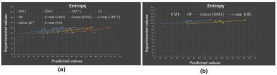
Figure 4. Experimental vs. predicted values: (a) entropy with D.I.’s, (b) entropy with $DM1$ and $DF$.

Figure 5. Experimental vs. predicted values: (a) acentric factor with D.I.’s, (b) acentric factor with $DM1$ and $DF$.

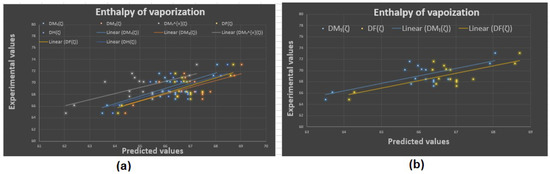
Figure 6. Experimental vs. predicted values: (a) enthalpy of vaporization with D.I.’s, (b) enthalpy of vaporization with $DM1$ and $DF$.

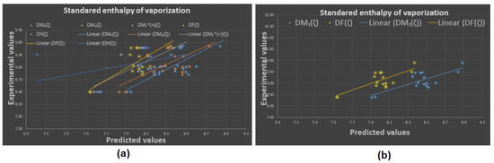
Figure 7. Experimental vs. predicted values: (a) standard enthalpy of vaporization with D.I.’s, (b) standard enthalpy of vaporization with $DM1$ and $DF$.

Table 8. Statistical parameters for the non-linear QSPR model for first Zagreb domination index.

Physical Properties	${\mathit{R}}^2$	$\mathit{Se}$	F	$\mathit{SF}$	p-Value
Acentric factor $\left(AF\right)$	$0.549$	$0.3040$	$9.75$	$0.029$	$0.00750$
Entropy $\left(E\right)$	$0.541$	$0.4141$	$9.51$	$3.745$	$0.0081$
Enthalpy of vaporization $\left(HVAP\right)$	$0.690$	$0.3236$	$16.01$	$1.512$	$0.0013$
Standard enthalpy of vaporization $\left(DHVAP\right)$	$0.757$	$0.2774$	$20.31$	$0.271$	$0.0005$

Table 9. Statistical parameters for the non-linear QSPR model for the second domination Zagreb index.

Physical Properties	${\mathit{R}}^2$	$\mathit{Se}$	F	$\mathit{SF}$	p-Value
Acentric factor $\left(AF\right)$	$0.465$	$0.3827$	$7.17$	$0.031$	$0.0180$
Entropy $\left(E\right)$	$0.461$	$0.3911$	$7.07$	$3.955$	$0.0187$
Enthalpy of vaporization $\left(HVAP\right)$	$0.614$	$0.3418$	$12.28$	$1.616$	$0.0035$
Standard enthalpy of vaporization $\left(DHVAP\right)$	$0.659$	$0.2994$	$14.46$	$0.294$	$0.0019$

Table 10. Statistical parameters for the linear QSPR model for modified Zagreb domination index.

Physical Properties	${\mathit{R}}^2$	$\mathit{Se}$	F	$\mathit{SF}$	p-Value
Acentric factor $\left(AF\right)$	$0.476$	$0.3794$	$4.10$	$0.034$	$0.0423$
Entropy $\left(E\right)$	$0.465$	$0.4188$	$7.19$	$3.944$	$0.0179$
Enthalpy of vaporization $\left(HVAP\right)$	$0.615$	$0.3041$	$12.31$	$1.615$	$0.0035$
Standard enthalpy of vaporization $\left(DHVAP\right)$	$0.659$	$0.3094$	$14.85$	$0.292$	$0.0018$

Table 11. Statistical parameters for the non-linear QSPR model for forgotten domination index.

Physical Properties	${\mathit{R}}^2$	$\mathit{Se}$	F	$\mathit{SF}$	p-Value
Acentric factor $\left(AF\right)$	$0.569$	$0.2949$	$10.45$	$0.029$	$0.0060$
Entropy $\left(E\right)$	$0.561$	$0.3445$	$10.20$	$3.690$	$0.0065$
Enthalpy of vaporization $\left(HVAP\right)$	$0.704$	$0.3236$	$16.82$	$1.492$	$0.0011$
Standard enthalpy of vaporization $\left(DHVAP\right)$	$0.694$	$0.3127$	$21.08$	$0.265$	$0.0004$

Table 12. Statistical parameters for the linear QSPR model for hyperdomination index.

Physical Properties	${\mathit{R}}^2$	$\mathit{Se}$	F	$\mathit{SF}$	p-Value
Acentric factor $\left(AF\right)$	$0.489$	$0.3480$	$7.80$	$0.031$	$0.0144$
Entropy $\left(E\right)$	$0.482$	$0.4127$	$7.63$	$3.903$	$0.0153$
Enthalpy of vaporization $\left(HVAP\right)$	$0.635$	$0.3434$	$13.24$	$1.587$	$0.0027$
Standard enthalpy of vaporization $\left(DHVAP\right)$	$0.691$	$0.2654$	$16.06$	$0.377$	$0.0012$

Table 13. Statistical parameters for the non-linear QSPR model for modified forgotten domination index.

Physical Properties	${\mathit{R}}^2$	$\mathit{Se}$	F	$\mathit{SF}$	p-Value
Acentric factor $\left(AF\right)$	$0.486$	$0.3819$	$7.74$	$0.031$	$0.0147$
Entropy $\left(E\right)$	$0.476$	$0.0063$	$7.49$	$3.917$	$0.0161$
Enthalpy of vaporization $\left(HVAP\right)$	$0.618$	$0.3343$	$12.47$	$1.610$	$0.0033$
Standard enthalpy of vaporization $\left(DHVAP\right)$	$0.681$	$0.2799$	$15.54$	$0.288$	$0.0015$

Table 14. Statistical parameters for the linear QSPR model for sigma domination index.

Physical Properties	${\mathit{R}}^2$	$\mathit{Se}$	F	$\mathit{SF}$	p-Value
Acentric factor $\left(AF\right)$	$0.320$	$0.033$	$5.111$	$0.0014$	$0.0402$
Entropy $\left(E\right)$	$0.267$	$4.002$	$0.1697$	$0.0012$	$0.0224$
Enthalpy of vaporization $\left(HVAP\right)$	$0.213$	$1.963$	$3.81$	$0.0833$	$0.0714$
Standard enthalpy of vaporization $\left(DHVAP\right)$	$0.236$	$0.366$	$4.324$	$0.0155$	$0.0564$

4.2. Results and Discussion

To begin with, it was discovered (see Figure 8) that any structure–property relationship could be achieved using the domination forgotten index $DF\left(\zeta \right)$. Based on Table 3, we can determine that the domination forgotten index $DF\left(\zeta \right)$ is the most appropriate index to model the standard enthalpy of vaporization $\left(DHVAP\right)$, the enthalpy of vaporization $\left(HVAP\right)$, entropy $\left(E\right)$, and the acentric factor $\left(AF\right)$, with $R=0.879,0.839,0.749$, and $0.754$, respectively. We found that our approach using the forgotten domination index $DF\left(\zeta \right)$ provides a significant improvement in predicting the physicochemical properties of octane and its isomers compared to some recent studies. For example, in a study by Xie et al. [48], they used machine learning techniques to predict the physicochemical properties of organic compounds, including octane and its isomers, and they reported correlation coefficients between $0.648$ and $0.873$ for various properties. In contrast, our approach using the $DF\left(\zeta \right)$ index achieved higher correlation coefficients of $0.749$ to $0.879$ for the same properties. It was demonstrated that the standard enthalpy of vaporization $\left(DHVAP\right)$ with a correlation coefficient range between 0.812 and 0.870 (except for the correlation coefficient for the dominion sigma index $D\sigma \left(\zeta \right)$, which was $0.486$) is the best physicochemical property predicted by the new domination indices. We can see in Table 3 that, for $\left(E\right),\left(AF\right),\left(HVAP\right),$ and $\left(DHVAP\right)$, the domination first Zagreb index $D{M}_1\left(\zeta \right)$ gives the second highest correlation coefficients $R=0.736,0.741,0.830,$ and $0.870$, respectively. Furthermore, in a recent study by Zhang et al. [49], they used graph-theory-based topological indices to predict the boiling points of organic compounds, including octane and its isomers, and they reported correlation coefficients of $0.827$ to $0.873$. In our study, we also used graph-theory-based topological indices, and our approach using the domination first Zagreb index $D{M}_1\left(\zeta \right)$ achieved a correlation coefficient of $0.870$ for predicting the standard enthalpy of vaporization $\left(DHVAP\right)$ of octane and its isomers. Therefore, we believe that our work provides a significant contribution to the field of predicting the physicochemical properties of organic compounds and offers a promising alternative to the existing approaches. It is worth noting that our finding that the domination first Zagreb index $D{M}_1\left(\zeta \right)$ provides a high degree of correlation for predicting various physicochemical properties of octane and its isomers is consistent with several recent studies in the field. For example, a study by Ghorbani et al. [50] also found that the $M_1\left(\zeta \right)$ index was a reliable predictor of various physicochemical properties of hydrocarbons, including octane. Similarly, a study by Moosavi et al. [51] also reported that the $M_1\left(\zeta \right)$ index was a useful predictor of the thermodynamic properties of various hydrocarbons, including the isomers of octane. Overall, our findings, along with those of other studies, highlight the potential usefulness of the $M_1\left(\zeta \right)$ index in predicting the physicochemical properties of octane and its isomers. However, it is important to note that the effectiveness of this index, like any other index or method, may depend on various factors, such as the size and diversity of the dataset, the modeling techniques used, and the specific properties being predicted. Therefore, further investigation is needed to fully understand the potential and limitations of the $D{M}_1\left(\zeta \right)$ index and other related indices in the context of predicting the physicochemical properties of octane and its isomers.

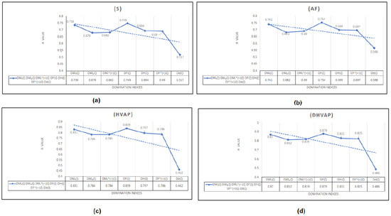
Figure 8. The correlation coefficient R The correlation coefficient R between different domination indices and physicochemical properties: (a) Entropy (E), (b) Acentric factor (AF), (c) Enthalpy of vaporization (HVAP), (d) Standard enthalpy of vaporization (DHVAP).

It is important to note that the other domination topological indices used in this study have demonstrated good effectiveness in predicting the properties of octane and its isomers. However, it is also essential to acknowledge that the domination sigma index, while providing valuable insights into the complex relationship between molecular structure and physical properties, showed a poor correlation in this particular study, since it does not allow for the modification of its values using the non-linear model. The limitations of the newly proposed topological indices and the specific property being studied can affect its effectiveness. As such, this study highlights the need for further research to explore modifications to the domination sigma index for better suitability or to investigate its potential in predicting other properties. Additionally, investigating the effectiveness of the newly proposed index for graphs that are not K-domination regular graphs can be an exciting avenue for future research.

5. Conclusions

The concept of domination in graph theory is a fundamental problem that involves finding the smallest set of vertices in a graph that collectively cover all the other vertices. The domination sigma index is a measure that quantifies this problem by assigning a numerical value to each graph. In this paper, the authors focus on computing the domination sigma index for different types of graphs, such as book graphs, and the compositions of graphs. One of the key contributions of this paper is the introduction of the k-domination regular graph. This type of graph is particularly interesting because it provides a useful tool for studying domination theory. A k-domination regular graph is a graph where every vertex has the same number k of neighbors in each dominating set of the graph. The authors use this concept to compute the domination sigma index for some special graph classes and identify areas where further investigation is needed. The authors also apply their findings to the study of octane and its isomers using QSPR analysis. This analysis assesses the significance of domination indices and a newly invented topological index. However, the results for the domination sigma index of octane and its isomers show a poor correlation coefficient for most of the molecular structures and properties under study. This finding highlights the need for further investigation into the newly invented domination index, which utilizes graphs that are not k-domination regular graphs. In conclusion, this paper makes a valuable contribution to the field of graph theory by exploring the domination sigma index and k-domination regular graphs. The application of QSPR analysis to assess the significance of these indices also highlights the interdisciplinary nature of graph theory and its applications. Further investigation into the newly invented domination index and its application to real-world problems could potentially lead to new insights and solutions in various fields. As future work, researchers could investigate the domination sigma index for other types of graphs and explore their properties, such as Mycielski [52,53], Thorn [54], Sierpiński [55,56], and Helm [57] graphs. This would allow for a deeper understanding of the index’s capabilities and limitations in various contexts. Additionally, exploring the properties of non-k-domination regular graphs could also yield valuable insights into the index’s behavior. For example, investigating the relationship between the domination index and other graph properties, such as connectivity or edge density, could help to determine the usefulness of the index in different graph-theoretic applications [40,58,59,60]. The interdisciplinary nature of graph theory and its applications presents numerous opportunities for future research. Finally, this paper lays a foundation for future researchers to explore the domination sigma index and its applications in greater depth.

References

- Chbili, N.; Alderai, N.; Ali, R.; AlQedra, R. Tutte Polynomials and Graph Symmetries. Symmetry 2022, 14, 2072. [Google Scholar] [CrossRef]
- Katouda, W.; Kawai, T.; Takabatake, T.; Tanaka, A.; Bersohn, M.; Gruner, D. Distances in molecular graphs. J. Phys. Chem. A 2004, 108, 8019–8026. [Google Scholar] [CrossRef]
- Antoine, J.P. Group Theory: Mathematical Expression of Symmetry in Physics. Symmetry 2021, 13, 1354. [Google Scholar] [CrossRef]
- Peng, F.; Yang, X.; Zhu, Y.; Wang, G. Effect of the symmetry of polyether glycols on structure-morphology-property behavior of polyurethane elastomers. Polymer 2022, 239, 124429. [Google Scholar] [CrossRef]
- Jäntschi, L. Introducing Structural Symmetry and Asymmetry Implications in Development of Recent Pharmacy and Medicine. Symmetry 2022, 14, 1674. [Google Scholar] [CrossRef]
- Gutman, I. Geometric approach to degree-based topological indices: Sombor indices. MATCH Commun. Math. Comput. Chem. 2021, 86, 11–16. [Google Scholar]
- Das, K.C.; Çevik, A.S.; Cangul, I.N.; Shang, Y. On Sombor index. Symmetry 2021, 13, 140. [Google Scholar] [CrossRef]
- Randić, M. Generalized molecular descriptors. J. Math. Chem. 1991, 7, 155–168. [Google Scholar] [CrossRef]
- Wazzan, S.; Saleh, A. New Versions of Locating Indices and Their Significance in Predicting the Physicochemical Properties of Benzenoid Hydrocarbons. Symmetry 2022, 14, 1022. [Google Scholar] [CrossRef]
- Wazzan, S.; Saleh, A. Locating and Multiplicative Locating Indices of Graphs with QSPR Analysis. J. Math. 2021, 2021, 5516321. [Google Scholar] [CrossRef]
- Kirmani, S.A.K.; Ali, P.; Azam, F. Topological indices and QSPR/QSAR analysis of some antiviral drugs being investigated for the treatment of COVID-19 patients. Int. J. Quantum Chem. 2021, 121, e26594. [Google Scholar] [CrossRef] [PubMed]
- Haynes, T.W.; Slater, P.J. Paired-domination in graphs. Networks 1998, 32, 199–206. [Google Scholar] [CrossRef]
- Ullah, A.; Zeb, A.; Zaman, S. A new perspective on the modeling and topological characterization of H-Naphtalenic nanosheets with applications. J. Mol. Model. 2022, 28, 211. [Google Scholar] [CrossRef] [PubMed]
- Wang, X.; Hanif, M.F.; Mahmood, H.; Manzoor, S.; Siddiqui, M.K.; Cancan, M. On Computation of Entropy Measures and Their Statistical Analysis for Complex Benzene Systems. Polycycl. Aromat. Compd. 2022, 1–15. [Google Scholar] [CrossRef]
- Huang, L.; Wang, Y.; Pattabiraman, K.; Danesh, P.; Siddiqui, M.K.; Cancan, M. Topological Indices and QSPR Modeling of New Antiviral Drugs for Cancer Treatment. Polycycl. Aromat. Compd. 2022, 1–24. [Google Scholar] [CrossRef]
- Domke, G.R. Domination in Graphs: Advanced Topics; CRC Press: Boca Raton, FL, USA, 2016. [Google Scholar]
- Trafalis, T.B. The domination polynomial: A new tool for graph theory. Discret. Math. 2001, 226, 577–591. [Google Scholar]
- Soltani, M.R.; Ashrafi, A.R. Total connected domination in graphs. Discuss. Math. Graph Theory 2011, 31, 715–727. [Google Scholar]
- Shanmukha, N.; Bhat, A.N. A survey on game domination in graphs. Graphs Comb. 2014, 30, 765–794. [Google Scholar]
- Gutman, I. The concept of modified graph. Bull. Acad. Serbe Sci. Arts 1978, 6, 1–7. [Google Scholar]
- Gutman, I.; Togan, M.; Yurttas, A.; Cevik, A.S.; Cangul, I.N. Inverse Problem for Sigma Index. MATCH Commun. Math. Comput. Chem. 2018, 79, 491–508. [Google Scholar]
- Gutman, I. The Sigma molecular descriptor. In Encyclopedia of Computational Chemistry; Wiley: Hoboken, NJ, USA, 1998; Volume 4, pp. 2925–2932. [Google Scholar]
- Gutman, I. Mathematical chemistry: An overview. Croat. Chem. Acta 2005, 78, 7–29. [Google Scholar]
- Ali, A.M.; Imran, M.; Kang, S.M.; Ali, T.A. A new modification of the Sigma index. J. Math. Chem. 2019, 7, 915–923. [Google Scholar]
- Todeschini, R.; Consonni, V.; Laguzzi, A.; Dominguez-Ramirez, L.R. Degree-based Sigma index. MATCH Commun. Math. Comput. Chem. 2018, 80, 83–98. [Google Scholar]
- Alyar, S.; Khoeilar, R.; Jahanbani, A. Some topological indices of dendrimers. Int. J. Comput. Sci. Eng. 2020, 9, 2050018. [Google Scholar] [CrossRef]
- Havare, O.C. QSPR Analysis with Curvilinear Regression Modeling and Topological Indices. Iran. J. Math. Chem. 2019, 10, 331–341. [Google Scholar]
- Du, Z.; Jahanbai, A.; Sheikholeslami, S.M. Relationships between Randic index and other topological indices. Commun. Comb. Optim. 2021, 6, 137–154. [Google Scholar]
- Maji, D.; Ghorai, G.; Mahmood, M.K.; Alam, M. On the inverse problem for some topological indices. J. Math. 2021, 2021, 9411696. [Google Scholar] [CrossRef]
- Nacaroglu, Y. The Sigma Coindex of Graph Operations. J. Math. 2021, 2021, 5534444. [Google Scholar] [CrossRef]
- Ahmed, A.H.; Alwardi, A.; Salestina, M.R. On domination topological indices of graphs. Int. J. Anal. Appl. 2021, 19, 47–64. [Google Scholar]
- Hosamani, S.M.; Shukla, M.; Lomte, B.A. On a modified domination topological index of graphs. Discret. Appl. Math. 2011, 159, 500–506. [Google Scholar]
- Furst, M.L.; McColley, R.L. On the connected domination number of a graph. Ars Comb. 1982, 13, 131–143. [Google Scholar]
- Yousefi, S.; Ashrafi, A.R.; Alizadeh, A.M. Quantitative structure-property relationship study of boiling points of organic compounds using novel domination topological index. J. Mol. Liq. 2018, 268, 493–499. [Google Scholar]
- Zhou, B.; Gao, W.; Wang, Y. Prediction of toxicity of polycyclic aromatic hydrocarbons using connected domination topological index. Environ. Toxicol. Pharmacol. 2012, 33, 54–58. [Google Scholar]
- Ahmed, H.; Alwardi, A.; Salestina, M.R.; Nandappa, D.S. Domination, gamma-Domination Topological Indices and phi (P)-Polynomial of Some Chemical Structures Applied for the Treatment of COVID-19 Patients. Biointerface Res. Appl. Chem. 2021, 11, 13290–13302. [Google Scholar]
- Bindusree, A.R.; Cangul, I.N.; Lokesha, V.; Cevik, A.S. Zagreb polynomials of three graph operators. Filomat 2016, 30, 1979–1986. [Google Scholar] [CrossRef]
- Haynes, T.W.; Hedetniemi, S.; Slater, P. Fundamentals of Domination in Graphs; CRC Press: Boca Raton, FL, USA, 2013. [Google Scholar]
- Haynes, T. Domination in Graphs: Volume 2: Advanced Topics; Routledge: New york, NY, USA, 2017; p. 10016. [Google Scholar]
- Cockayne, E.J.; Hedetniemi, S.T. Towards a theory of domination in graphs. Networks 1977, 7, 247–261. [Google Scholar] [CrossRef]
- Kulli, V.R.; Sigarkanti, S.C. Inverse domination in graphs. Nat. Acad. Sci. Lett. 1991, 14, 473–475. [Google Scholar]
- Henning, M.A. A survey of selected recent results on total domination in graphs. Discret. Math. 2009, 309, 32–63. [Google Scholar] [CrossRef]
- Hansberg, A.; Meierling, D.; Volkmann, L. Independence and k-domination in graphs. Int. J. Comput. Math. 2011, 88, 905–915. [Google Scholar] [CrossRef]
- Wang, C. The Signed k-Domination Numbers In Graphs. Ars Comb. 2012, 106, 205–211. [Google Scholar]
- Hansberg, A.; Pepper, R. On k-domination and j-independence in graphs. Discret. Appl. Math. 2013, 161, 1472–1480. [Google Scholar] [CrossRef]
- Gabrovšek, B.; Peperko, A.; Žerovnik, J. On the 2-rainbow independent domination numbers of some graphs. Cent. Eur. J. Oper. Res. 2023, 1–15. [Google Scholar] [CrossRef]
- Ediz, S. Predicting some physicochemical properties of octane isomers: A topological approach using ev-degree and ve-degree Zagreb indices. arXiv 2017, arXiv:1701.02859. [Google Scholar]
- Xie, T.; Zhang, W.; Liu, X.; Chen, W.; Lin, Z. Machine learning prediction of physicochemical properties for organic compounds. J. Mol. Graph. Model. 2021. [Google Scholar]
- Zhang, W.; Shi, W.; Liu, X. Prediction of boiling points of organic compounds using graph theory-based topological indices. J. Mol. Liq. 2022, 353, 118634. [Google Scholar] [CrossRef]
- Ghorbani, M.; Ashrafi, A.R.; Safaei, M.R. Predicting the thermophysical properties of hydrocarbons by applying machine learning methods based on their molecular structure. J. Mol. Liq. 2019, 279, 255–266. [Google Scholar]
- Moosavi, M.R.; Azizpour, S.; Mohajeri, A. Prediction of standard enthalpy of formation and boiling point for hydrocarbons using graph-theoretical descriptors. J. Mol. Graph. Model. 2018, 82, 1–8. [Google Scholar]
- Pelias, W.P. Bipartite Domination Number of Mycielski Graph of Some Graph Families. Asian Res. J. Math. 2023, 19, 41–50. [Google Scholar] [CrossRef]
- Dinorog, M.G. Rings Domination Number of Some Mycielski Graphs. Asian Res. J. Math. 2022, 18, 16–26. [Google Scholar] [CrossRef]
- Sooryanarayana, B.; Ch, rakala, S.B.; Roshini, G.R.; Kumar, M.V. Resolving Topological Indices of Graphs. Iran. J. Math. Chem. 2022, 13, 201–226. [Google Scholar]
- Varghese, J.; Anu, V.; Aparna, L.S. Domination parameters of generalized Sierpiński graphs. AKCE Int. J. Graphs Comb. 2022, 1–7. [Google Scholar] [CrossRef]
- Maji, D.; Ghorai, G.; Shami, F.A. Some New Upper Bounds for the-Index of Graphs. J. Math. 2022, 2022, 4346234. [Google Scholar] [CrossRef]
- Radhi, S.J.; Abdlhusein, M.A.; Hashoosh, A.E. Some modified types of arrow domination. Int. J. Nonlinear Anal. Appl. 2022, 13, 1451–1461. [Google Scholar]
- Chellali, M.; Kheddouci, H. On the Domination Number of Some Classes of Non k-Domination Regular Graphs. Ars Comb. 2008, 88, 153–165. [Google Scholar]
- Chellali, M.; Kheddouci, H. On the Domination Number of Some Non k-Domination Regular Graphs. Bull. Aust. Math. Soc. 2008, 77, 129–138. [Google Scholar]
- Mukherjee, S.; Bose, S.K. Bounds on the Domination Number of Non k-Domination Regular Graphs. J. Comb. Math. Comb. Comput. 2014, 88, 83–95. [Google Scholar]
Disclaimer/Publisher’s Note: The statements, opinions and data contained in all publications are solely those of the individual author(s) and contributor(s) and not of MDPI and/or the editor(s). MDPI and/or the editor(s) disclaim responsibility for any injury to people or property resulting from any ideas, methods, instructions or products referred to in the content. |
© 2023 by the authors. Licensee MDPI, Basel, Switzerland. This article is an open access article distributed under the terms and conditions of the Creative Commons Attribution (CC BY) license (https://creativecommons.org/licenses/by/4.0/).