On the Splitting Tensor of the Weak f-Contact Structure

Abstract

A weak f-contact structure, introduced in our recent works, generalizes the classical f-contact structure on a smooth manifold, and its characteristic distribution defines a totally geodesic foliation with flat leaves. We find the splitting tensor of this foliation and use it to show positive definiteness of the Jacobi operators in the characteristic directions and to obtain a topological obstruction (including the Adams number) to the existence of weak f-K-contact manifolds, and prove integral formulas for a compact weak f-contact manifold. Based on applications of the weak f-contact structure in Riemannian contact geometry considered in the article, we expect that this structure will also be fruitful in theoretical physics, e.g., in QFT.

1. Introduction

After many results in classical mechanics related to contact transformations, the famous Boothby-Wang fibration of 1958 marked the beginning of the theory of contact manifolds [1]. Important examples of contact manifolds are the principal circle bundles and the tangent sphere bundles, e.g., [2]. The growing interest in Riemannian contact geometry is associated with its important role in differential equations, differential geometry and topology, as well as in physics, e.g., geometrical optics, classical and quantum mechanics, thermodynamics, integrable systems and control theory.

A framed f-structure on a $(2n+s)$-dimensional Riemannian manifold is defined by a (1,1)-tensor f of constant rank $2n$, which satisfies $f^3+f=0$, and linearly independent vector fields ${\left\{{\xi }_i\right\}}_{1\le i\le s}$ spanning $kerf$—the characteristic distribution, see [3,4,5,6,7,8,9,10]. This higher dimensional analog of almost contact ($s=1$) and almost complex ($s=0$) structures appears naturally when studying hypersurfaces of almost contact manifolds, see [11], and submanifolds of almost complex manifolds [12]. Moreover, many space-time manifolds can be endowed with framed f-structures, see [13]. The importance of the tensor field f stems from the fact that its existence is equivalent to the reduction of the structure group of the manifold to $U\left(n\right)\times O\left(s\right)$, see [3].

An interesting case occurs when $kerf$ is parallelizable or is defined by a homomorphism of an s-dimensional Lie algebra $\mathfrak{g}$ to the Lie algebra of all vector fields on M, i.e., M admits a $\mathfrak{g}$-foliation, see [14]. In the presence of a compatible metric, such $\mathfrak{g}$-foliations are totally geodesic foliations spanned by Killing vector fields, e.g., [15]. For a 1-dimensional Lie algebra, a $\mathfrak{g}$-foliation is generated by a nonvanishing vector field, and we get contact metric manifolds as well as K-contact and Sasakian ones, see [2].

The f-K-contact structure (i.e., an f-contact structure, whose characteristic vector fields generate 1-parameter groups of isometries), see [16], generalizes the $\mathcal{K}$-contact structure of [3] (i.e., $s=1$), both structures can be regarded as intermediate between a framed f-structure and S-structure (Sasaki structure when $s=1$). In [17], conditions are found under which a given compact f-K-contact manifold is a mapping torus of such a manifold of lower dimension. Various symmetries of contact and framed f-manifolds are studied, e.g., in [18], and sufficient conditions are considered when an f-contact manifold carries a canonical metric, such as Einstein-type or constant curvature, or admits a local decomposition (splitting), in [4,19,20].

The characteristic distribution $kerf$ of an f-contact structure defines a totally geodesic foliation. Such foliations have simple extrinsic geometry, i.e., vanishing second fundamental form of the leaves, and appear on (sub)manifolds with degenerate differential forms and curvature-like tensors, e.g., [21]. The splitting tensor (or, co-nullity tensor) of a foliation is a useful tool to study totally geodesic foliations, and to obtain integral formulas, e.g., [21]. Integral formulas are a powerful tool for proving global results in analysis and geometry. There are series of integral formulas for two orthogonal complementary distributions (beginning with Reeb’s formula for foliations of codimension one), which involve the Newton transformations of splitting tensor and certain components of the curvature tensor, and are used to solve many problems (see, surveys in [21,22,23]): (i) the existence and characterizing of foliations, whose leaves have a given geometric property, such as being totally geodesic, totally umbilical or minimal; (ii) prescribing the higher mean curvatures of the leaves of a foliation; (iii) minimizing functionals such as volume and energy defined for tensor fields on a foliated manifold.

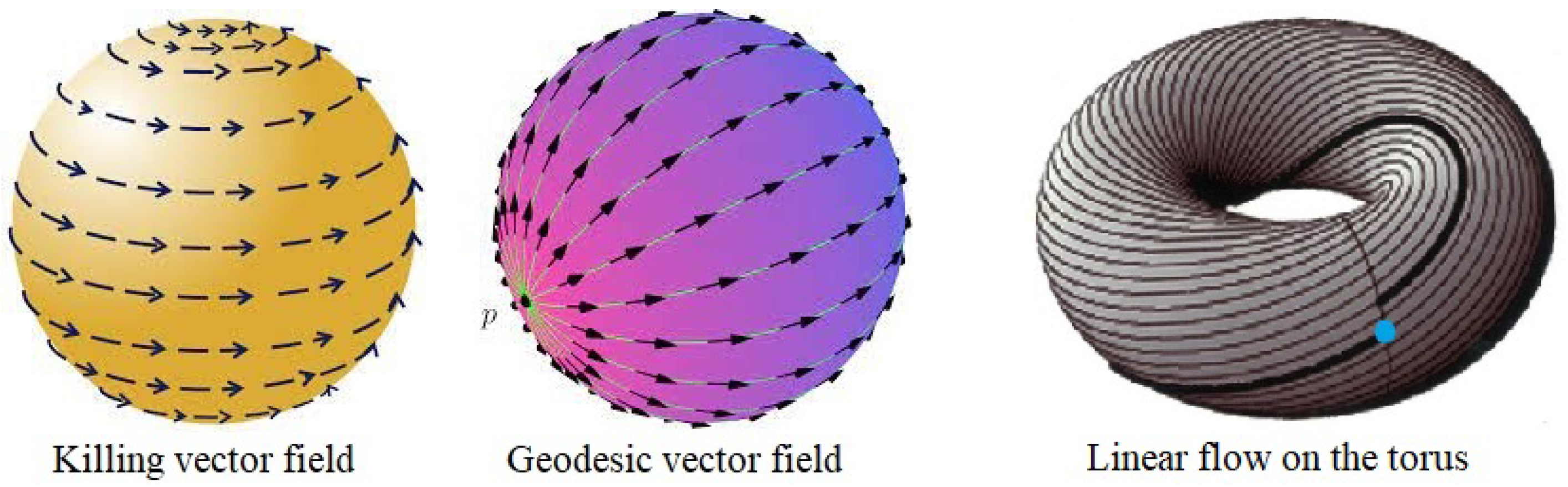
In [24,25] the study of “weak” contact structures on a smooth $(2n+s)$-dimensional manifold (i.e., the complex structure on the characteristic distribution is replaced with a nonsingular skew-symmetric tensor) was initiated. These structures generalize an f-contact structure and its satellites, and allow a new look at the Riemannian classical theory and find its new applications, for example, to build manifolds with Killing vector fields and totally geodesic foliations, (well known examples are flows on the sphere, linear flow on the torus, see Figure 1), to produce Riemannian manifolds with positive $\xi$-sectional curvature, and to investigate Einstein-type metrics.

In [25], we retracted weak structures with positive partial Ricci curvature onto the subspace of classical structures of the same type. In [24], we proved that the $\mathcal{S}$-structure is rigid, i.e., our weak $\mathcal{S}$-structure is the $\mathcal{S}$-structure, and a metric weak f-structure with parallel tensor f is the weak $\mathcal{C}$-structure. The characteristic distribution of the weak f-contact structure (and its particular case—the weak f-K-contact structure) is integrable and defines a totally geodesic foliation. The splitting tensor of a totally geodesic foliation is important in studying c-nullity foliations of Riemannian manifolds M (given by $\{X\in TM:R_{X,Y}=c(X\wedge Y)\}$) and relative nullity foliations of Riemannian submanifolds (given by $\{X\in TM:\beta (X,·)=0\}$, where $\beta$ is the second fundamental form), e.g., [26], and in integral formulas for foliations and Riemannian almost product manifolds, see [21].

The article continues our study [24,25] of the geometry of weak f-contact manifolds. Our achievement is the generalization of some results on f-contact manifolds to the case of weak f-contact manifolds and demonstration of the usefulness of this weak structure for the study of totally geodesic foliations, Killing vector fields and the corresponding splitting tensors on Riemannian manifolds. The proofs use the properties of new tensors, as well as the constructions required in the classical case.

The article is organized as follows. In Section 2, following the introductory Section 1, we recall some results regarding framed weak f-manifolds. Section 3 contains the main results and consists of three parts. In Section 3.1, we study the geometry of weak f-contact manifolds and show that they are endowed with totally geodesic foliations with flat fibers (Proposition 2). In Section 3.2, we find the splitting tensor for the characteristic foliation of weak f-contact manifolds (Theorem 1), and use it to show positive definiteness of the Jacobi operators in the characteristic directions, or, equivalently, that the $\xi$-sectional curvature is positive (Theorem 2) and to obtain a topological obstruction, including the Adams number, to the existence of weak f-K-contact manifolds (Theorem 3), and prove integral formulas for compact weak f-contact manifolds (Proposition 4).

2. Preliminaries

Here, we recall the basics of the weak f-contact structure (see [24,25]) as a higher dimensional analog of the weak almost contact structure.

Aframed weak structure on a smooth manifold $M^{2n+s}$ is the set $(f,Q,{\xi }_i,{\eta }^i)$, where f is a $(1,1)$-tensor, Q is a nonsingular $(1,1)$-tensor, ${\xi }_i(1\le i\le s)$ are characteristic vector fields, which form the characteristic distribution, and ${\eta }^i$ are dual 1-forms, satisfying

$$f^2=-Q+{\sum }_i{\eta }^i\otimes {\xi }_i,{\eta }^i\left({\xi }_j\right)={\delta }_j^i,Q{\xi }_i={\xi }_i.$$

(1)

Thus, $f^3+fQ=0$. The forms ${\eta }^i$ are linearly independent and determine a smooth $2n$-dimensional contact distribution $\mathcal{D}:={\bigcap }_{i}ker{\eta }^i$ (the collection of subspaces ${\mathcal{D}}_m=\{X\in T_{m}M:{\eta }^i\left(X\right)=0,1\le i\le s\}$ for $m\in M$). We assume that $\mathcal{D}$ is f-invariant,

$$fX\in \mathcal{D}(X\in \mathcal{D}),$$

(2)

as in the theory of framed f-structure [3,9], where $Q=\mathrm{id}$—the identity map of $TM$. For a framed weak f-structure on a smooth manifold M, the tensor f has rank $2n$ and

$$f{\xi }_i=0,{\eta }^i\circ f=0,{\eta }^i\circ Q={\eta }^i,[Q,f]=0;$$

thus, $\mathcal{D}=f\left(TM\right)$. By (1) and (2), the distribution $\mathcal{D}$ is invariant for Q: $Q\left(\mathcal{D}\right)=\mathcal{D}$.

Let g be a compatible (or, associated) Riemannian metric on $M^{2n+s}(f,Q,{\xi }_i,{\eta }^i)$, i.e.,

$$\begin{array}{c}\hfill g(fX,fY)=g(X,QY)-{\sum }_i{\eta }^i\left(X\right){\eta }^i\left(Y\right),X,Y\in {\mathfrak{X}}_M.\end{array}$$

(3)

Then $(f,Q,{\xi }_i,{\eta }^i,g)$ is called a weak metric structure on M, and $M(f,Q,{\xi }_i,{\eta }^i,g)$ is called a weak metricmanifold. Putting $Y={\xi }_i$ in (3) and using $Q{\xi }_i={\xi }_i$, we get

$$\begin{array}{c}\hfill {\eta }^i\left(X\right)=g(X,{\xi }_i)(i=1,\dots ,s).\end{array}$$

In particular, $kerf$ and $\mathcal{D}$ are additionally orthogonal distributions.

For a weak metric f-structure, the contact distribution $\mathcal{D}$ is nowhere integrable, since for a nonzero $X\perp kerf$ we get

$$g([X,fX],{\xi }_i)=2d{\eta }^i(fX,X)=g(fX,fX)>0.$$

For a weak metric f-structure, the tensor f is skew-symmetric (the same for a metric f-structure) and Q is self-adjoint, see [25].

Remark 1.

There exists a compatible metric on any framed f-manifold, e.g., [3]. A framed weak f-manifold admits a compatible metric if f in (1)–(2) has a skew-symmetric representation, i.e., for any $x\in M$ there exist a neighborhood $U_x\subset M$ and a frame $\left\{e_i\right\}$ on $U_x$, for which f has a skew-symmetric matrix, see [25]. By (3), we get $g(X,QX)=g(fX,fX)>0$ for any nonzero vector $X\perp kerf$; thus, the tensor Q is positive definite.

A framed (weak) f-structure is called normal if the following tensor is zero:

$$\begin{array}{c}\hfill N^{\left(1\right)}(X,Y)=[f,f](X,Y)+2{\sum }_{i}d{\eta }^i(X,Y){\xi }_i,X,Y\in {\mathfrak{X}}_M,\end{array}$$

where the Nijenhuis torsion $[f,f]$ of f is given by

$$\begin{array}{c}\hfill [f,f](X,Y)=f^2[X,Y]+[fX,fY]-f[fX,Y]-f[X,fY],X,Y\in {\mathfrak{X}}_M,\end{array}$$

(4)

and the exterior derivative of a differential form ${\eta }^i$ is given by

$$d{\eta }^i(X,Y)=\frac{1}{2}\{X\left({\eta }^i\left(Y\right)\right)-Y\left({\eta }^i\left(X\right)\right)-{\eta }^i\left([X,Y]\right)\},X,Y\in {\mathfrak{X}}_M.$$

(5)

Recall the following formulas with the Lie derivative ${\pounds }_Z$ in the Z-direction:

$$\begin{array}{cc}\hfill \left({\pounds }_{Z}f\right)X& =[Z,fX]-f[Z,X](X,Y\in {\mathfrak{X}}_M),\hfill \end{array}$$

(6)

$$\begin{array}{cc}\hfill \left({\pounds }_{{\xi }_i}g\right)(X,Y)& ={\xi }_i\left(g(X,Y)\right)-g([{\xi }_i,X],Y)-g(X,[{\xi }_i,Y]).\hfill \end{array}$$

(7)

The following tensors $N_i^{\left(2\right)},N_i^{\left(3\right)}$ and $N_{ij}^{\left(4\right)}$ are well known, see [3,9] and (5):

$$\begin{array}{cc}\hfill N_i^{\left(2\right)}(X,Y)& =\left({\pounds }_{fX}{\eta }^i\right)\left(Y\right)-\left({\pounds }_{fY}{\eta }^i\right)\left(X\right)=2d{\eta }^i(fX,Y)-2d{\eta }^i(fY,X),\hfill \\ \hfill N_i^{\left(3\right)}\left(X\right)& =\left({\pounds }_{{\xi }_i}f\right)X=[{\xi }_i,fX]-f[{\xi }_i,X],\hfill \\ \hfill N_{ij}^{\left(4\right)}\left(X\right)& =\left({\pounds }_{{\xi }_i}{\eta }^j\right)\left(X\right)={\xi }_i\left({\eta }^j\left(X\right)\right)-{\eta }^j\left([{\xi }_i,X]\right)=2d{\eta }^j({\xi }_i,X).\hfill \end{array}$$

For $s=1$, these tensors reduce to certain tensors on (weak) almost contact manifolds:

$$\begin{array}{c}\hfill N^{\left(2\right)}(X,Y)=\left({\pounds }_{fX}\eta \right)Y-\left({\pounds }_{fY}\eta \right)X,N^{\left(3\right)}={\pounds }_{\xi }f,N^{\left(4\right)}={\pounds }_{\xi }\eta .\end{array}$$

Remark 2.

Let $M^{2n+s}(f,Q,{\xi }_i,{\eta }^i)$ be a framed weak f-manifold. Consider the product manifold $\overline{M}=M^{2n+s}\times {\mathbb{R}}^s$, where ${\mathbb{R}}^s$ is a Euclidean space with a basis ${\partial }_1,\dots ,{\partial }_s$, and define tensors $\overline{f}$ and $\overline{Q}$ on $\overline{M}$ putting

$$\begin{array}{cc}\hfill \overline{f}(X,{\sum }_i{a}^i{\partial }_i)& =(fX-{\sum }_i{a}^i{\xi }_i,{\sum }_j{\eta }^j\left(X\right){\partial }_j),\hfill \\ \hfill \overline{Q}(X,{\sum }_i{a}^i{\partial }_i)& =(QX,{\sum }_i{a}^i{\partial }_i).\hfill \end{array}$$

Hence, $\overline{f}(X,0)=(fX,0)$, $\overline{Q}(X,0)=(QX,0)$ for $X\perp kerf$, $\overline{f}({\xi }_i,0)=(0,{\partial }_i)$, $\overline{Q}({\xi }_i,0)=({\xi }_i,0)$ and $\overline{f}(0,{\partial }_i)=(-{\xi }_i,0)$, $\overline{Q}(0,{\partial }_i)=(0,{\partial }_i)$. Then, it is easy to verify that ${\overline{f}}^2=-\overline{Q}$. The tensors $N^{\left(1\right)},N_i^{\left(2\right)},N_i^{\left(3\right)}$ and $N_{ij}^{\left(4\right)}$ appear when we derive the integrability condition $[\overline{f},\overline{f}]=0$ (vanishing of the Nijenhuis torsion of $\overline{f}$ ) and express the normality condition $N^{\left(1\right)}=0$ of a framed weak f-structure on M.

3. Results

In Section 3.1, we introduce the weak f-contact structure and its important case—the weak f-K-contact structure, which generalize the f-contact and f-K-contact structures, and show that the distribution $kerf$ is integrable and defines a totally geodesic foliation with flat leaves. In Section 3.2, we derive the splitting tensor of such structures and give its applications. In Section 3.3, we study integral formulas involving the splitting tensor on weak f-contact manifolds.

3.1. Geometry of Weak f-Contact Manifolds

The following definition is a copy of the classical definition, for example, [16].

Definition 1.

A weak f-contact structure is a weak metric f-structure satisfying

$$\begin{array}{c}\hfill \Phi =d{\eta }^1=\dots =d{\eta }^s,\end{array}$$

(8)

(thus, $d\Phi =0$), where $\Phi (X,Y)=g(X,fY)(X,Y\in {\mathfrak{X}}_M)$ is called the fundamental 2-form. A weak f-contact structure is called a weak f-K-contact structure if each characteristic vector field ${\xi }_i$ is Killing, i.e., ${\pounds }_{{\xi }_i}g=0$, see (7). A normal weak f-contact manifold is called a weak $\mathcal{S}$-manifold.

The relationships between the different classes of weak manifolds (considered in this article) can be summarized in the well-known diagram for classical structures:

$$\left|\begin{array}{c}\mathrm{framed}\mathrm{weak}\\ f-\mathrm{manifold}\end{array}\right|\stackrel{metric}{⟶}\left|\begin{array}{c}\mathrm{metric}\mathrm{weak}\\ f-\mathrm{manifold}\end{array}\right|\stackrel{\Phi =d{\eta }^i}{⟶}\left|\begin{array}{c}\mathrm{weak}\\ f-\mathrm{contact}\end{array}\right|\stackrel{{\xi }_i-Killing}{⟶}\left|\begin{array}{c}\mathrm{weak}\\ f-\mathrm{K}-\mathrm{contact}\end{array}\right|.$$

For $s=1$, we get the following diagram:

$$\left|\begin{array}{c}\mathrm{weak}\mathrm{almost}\\ \mathrm{contact}\end{array}\right|\stackrel{metric}{⟶}\left|\begin{array}{c}\mathrm{weak}\mathrm{almost}\\ \mathrm{contact}\mathrm{metric}\end{array}\right|\stackrel{\Phi =d\eta }{⟶}\left|\begin{array}{c}\mathrm{weak}\mathrm{contact}\\ \mathrm{metric}\end{array}\right|\stackrel{\xi -Killing}{⟶}\left|\begin{array}{c}\mathrm{weak}\\ \mathrm{K}-\mathrm{contact}\end{array}\right|.$$

Remark 3.

(a) 

In [5], an f-contact manifold was called an almost $\mathcal{S}$-manifold. Analogously, in [24], a weak f-contact manifold was called a weak almost $\mathcal{S}$-manifold. For $s=1$, a weak (almost) $\mathcal{S}$-manifold is a weak (almost) Sasakian manifold, see [3].

(b) 

For a weak f-contact manifold, the tensors $N_i^{\left(2\right)}$ and $N_{ij}^{\left(4\right)}$ vanish; moreover, $N_i^{\left(3\right)}$ vanishes if and only if ${\xi }_i$ is a Killing vector field, see ([24], Theorem 2.2).

The (1,1)-tensor $\tilde{Q}=Q-\mathrm{id}$ is useful for weak f-contact manifolds. Note that $\tilde{Q}=0$ is true for f-contact manifolds. We get $[\tilde{Q},f]=0$ and $\tilde{Q}{\xi }_i=0$.

Remark 4.

The Levi-Civita connection ∇ of a Riemannian metric g is given by

$$\begin{array}{cc}\hfill 2g({\nabla }_{X}Y,Z)& =Xg(Y,Z)+Yg(X,Z)-Zg(X,Y)\hfill \\ \hfill & +g\left(\right[X,Y],Z)+g\left(\right[Z,X],Y)-g\left(\right[Y,Z],X),\hfill \end{array}$$

and has the properties, for example, [21,27],

$$\begin{array}{cc}& Xg(Y,Z)=g({\nabla }_{X}Y,Z)+g(Y,{\nabla }_{X}Z)\left(\mathrm{metric}\mathrm{compatible}\right),\\ & [X,Y]={\nabla }_{X}Y-{\nabla }_{Y}X\left(\mathrm{without}\mathrm{torsion}\right).\end{array}$$

Proposition 1.

(see Corollary 2.1 in [24]). For a weak f-contact structure, we get

$$\begin{array}{ccc}\hfill g(\left({\nabla }_{X}f\right)Y,Z)& =& \frac{1}{2}g(N^{\left(1\right)}(Y,Z),fX)+g(fX,fY)\overline{\eta }\left(Z\right)-g(fX,fZ)\overline{\eta }\left(Y\right)\hfill \\ \hfill & +& \frac{1}{2}{N}^{\left(5\right)}(X,Y,Z),\hfill \end{array}$$

(9)

where $\overline{\eta }={\sum }_i{\eta }^i$, and a skew-symmetric with respect to Y and Z tensor $N^{\left(5\right)}(X,Y,Z)$ is given by

$$\begin{array}{cc}\hfill & N^{\left(5\right)}(X,Y,Z)=\left(fZ\right)\left(g(X,\tilde{Q}Y)\right)-\left(fY\right)\left(g(X,\tilde{Q}Z)\right)\hfill \\ \hfill & +g([X,fZ],\tilde{Q}Y)-g([X,fY],\tilde{Q}Z)+g([Y,fZ]-[Z,fY]-f[Y,Z],\tilde{Q}X).\hfill \end{array}$$

Only one new tensor $N^{\left(5\right)}$ (vanishing at $\tilde{Q}=0$), which supplements the sequence of well-known tensors $N^{\left(i\right)},i=1,2,3,4$, is needed to study the weak f-contact structure. For a weak metric f-structure, the tensor $N^{\left(5\right)}$ is more complicated, see ([24], Proposition 2.3). For a weak f-contact structure, we find particular values of the tensor $N^{\left(5\right)}$:

$$\begin{array}{c}{N}^{\left(5\right)}(X,{\xi }_i,Z)=-N^{\left(5\right)}(X,Z,{\xi }_i)=g(N_i^{\left(3\right)}\left(Z\right),\tilde{Q}X),\hfill \\ N^{\left(5\right)}({\xi }_i,Y,Z)=g\left(\right[{\xi }_i,fZ],\tilde{Q}Y)-g\left(\right[{\xi }_i,fY],\tilde{Q}Z),\hfill \\ N^{\left(5\right)}({\xi }_i,{\xi }_j,Y)=N^{\left(5\right)}({\xi }_i,Y,{\xi }_j)=0.\hfill \end{array}$$

(10)

A distribution $\tilde{\mathcal{D}}\subset TM$ is called totally geodesic if ${\nabla }_{X}Y+{\nabla }_{Y}X\in \tilde{\mathcal{D}}$ for any vector fields $X,Y\in \tilde{\mathcal{D}}$ – this is the case when any geodesic of M that is tangent to $\tilde{\mathcal{D}}$ at one point is tangent to $\tilde{\mathcal{D}}$ at all its points, e.g., ([21], Section 1.3.1). An integrable (i.e., tangent to a foliation) and totally geodesic distribution determines a totally geodesic foliation.

The Riemannian curvature tensor is given by the expression, see [27],

$$R_{X,Y}Z={\nabla }_X{\nabla }_{Y}Z-{\nabla }_Y{\nabla }_{X}Z-{\nabla }_{[X,Y]}Z.$$

Proposition 2.

For the weak f-contact structure, the characteristic distribution $kerf$ is tangent to a totally geodesic foliation with flat leaves (that is $R_{{\xi }_i,{\xi }_j}{\xi }_k=0)$.

Proof. 

We need to prove the following equality (from which $R_{{\xi }_i,{\xi }_j}{\xi }_k=0$ follows):

$$\begin{array}{c}\hfill {\nabla }_{{\xi }_i}{\xi }_j=0,1\le i,j\le s.\end{array}$$

(11)

Taking $X={\xi }_i$ in (9) and using (10)${}_2$, we get

$$\begin{array}{c}\hfill 2g(\left({\nabla }_{{\xi }_i}f\right)Y,Z)=g([{\xi }_i,fZ],\tilde{Q}Y)-g([{\xi }_i,fY],\tilde{Q}Z),1\le i\le s.\end{array}$$

(12)

Then, taking $Y={\xi }_j$ in (12), we get $f{\nabla }_{{\xi }_i}{\xi }_j=0$, that is ${\nabla }_{{\xi }_i}{\xi }_j$ is orthogonal to $\mathcal{D}$. Also,

$${\eta }^k\left([{\xi }_i,{\xi }_j]\right)=-2d{\eta }^k({\xi }_i,{\xi }_j)=-2g({\xi }_i,f{\xi }_j)=0;$$

hence, $[{\xi }_i,{\xi }_j]=0$, i.e., ${\nabla }_{{\xi }_i}{\xi }_j={\nabla }_{{\xi }_j}{\xi }_i$. From $g({\xi }_j,{\xi }_k)={\delta }_{jk}$, using the covariant derivative with respect to ${\xi }_i$ and the above equality, we get ${\nabla }_{{\xi }_i}{\xi }_j\underline{\in \mathcal{D}}$. Thus, (11) is true. By (11), the distribution $kerf$ is integrable (i.e., $[X,Y]={\nabla }_{X}Y-{\nabla }_{Y}X$ belongs to $\mathcal{D}$ for any vector fields $X,Y$ from $\mathcal{D}$) and totally geodesic (i.e., ${\nabla }_{X}Y+{\nabla }_{Y}X$ belongs to $\mathcal{D}$ for any vector fields $X,Y$ from $\mathcal{D}$) with flat leaves.  □

Remark 5.

(i) Proposition 2 was proved in ([24], Section 2) for some special cases of weak f-contact manifolds. The proof that ${\nabla }_{{\xi }_i}{\xi }_j$ is orthogonal to $\mathcal{D}$ requires some calculations with the tensor $N^{\left(5\right)}$. (ii) By (8) we get $g([X,{\xi }_i],{\xi }_k)=2d{\eta }^k({\xi }_i,X)=2\Phi ({\xi }_i,X)=0$. Using this and (11) gives the following equality for the weak f-contact structure:

$$\begin{array}{c}\hfill g({\nabla }_X{\xi }_i,{\xi }_k)=g({\nabla }_{{\xi }_i}X,{\xi }_k)=-g({\nabla }_{{\xi }_i}{\xi }_k,X)=0,X\in TM,1\le i,k\le s.\end{array}$$

(13)

3.2. The Splitting Tensor of a Weak f-Contact Manifold

For a weak f-contact manifold, the splitting tensor (or, co-nullity tensor) $C:kerf\times \mathcal{D}\to \mathcal{D}$ is defined by

$$C_{\xi }\left(X\right)=-P\left({\nabla }_X\xi \right),X\in \mathcal{D},\xi \in kerf,\parallel \xi \parallel =1,$$

where $P:TM\to \mathcal{D}$ is the orthoprojector. Since $kerf$ defines a totally geodesic foliation, see Proposition 2, then the distribution $\mathcal{D}$ is totally geodesic if and only if $C_{\xi }$ is skew-symmetric, and $\mathcal{D}$ is integrable if and only if $C_{\xi }$ is symmetric.

Thus, $C_{\xi }\equiv 0$ if and only if $\mathcal{D}$ is integrable and defines a totally geodesic foliation; in this case, by de Rham Decomposition Theorem, the manifold splits (is locally the product of Riemannian manifolds defined by distributions $\mathcal{D}$ and $kerf$), e.g., [21]. The self-adjoint shape operator $A_{\xi }$ and the skew-symmetric operator $T_{\xi }$, on $\mathcal{D}$ are given by

$$A_{\xi }=(1/2)(C_{\xi }+C_{\xi }^{*}),T_{\xi }=(1/2)(C_{\xi }-C_{\xi }^{*}),$$

(14)

where ${}^{*}$ is the conjugation of a (1,1)-tensor. Thus, the splitting tensor is decomposed as

$$C_{\xi }=A_{\xi }+T_{\xi }$$

(15)

into the sum of skew-symmetric and self-adjoint tensors dual to (1,2)-tensors: the second fundamental form and the integrability tensor, respectively [21]. If $\mathcal{D}$ is integrable (tangent to a foliation), then $C_{\xi }=A_{\xi }$, and if $\mathcal{D}$ is totally geodesic, then $C_{\xi }=T_{\xi }$.

The tensors $N_i^{\left(3\right)}$ are important for f-contact manifolds. Therefore, we define for a weak f-contact manifold the tensor field $h=(h_1,\dots ,h_s)$, where

$$\begin{array}{c}\hfill h_i=(1/2)N_i^{\left(3\right)}=(1/2){\pounds }_{{\xi }_i}f.\end{array}$$

By Remark 3b, $h_i=0$ if and only if ${\xi }_i$ is a Killing vector field. Next, we calculate

$$\begin{array}{cc}\hfill \left({\pounds }_{{\xi }_i}f\right)X& ={\nabla }_{{\xi }_i}\left(fX\right)-{\nabla }_{fX}{\xi }_i-f({\nabla }_{{\xi }_i}X-{\nabla }_X{\xi }_i)\hfill \\ \hfill & =\left({\nabla }_{{\xi }_i}f\right)X-{\nabla }_{fX}{\xi }_i+f{\nabla }_X{\xi }_i.\hfill \end{array}$$

(16)

Taking $X={\xi }_i$ in (16) and using ${\nabla }_{{\xi }_i}{\xi }_j=0$ and $\left({\nabla }_{{\xi }_i}f\right){\xi }_j$ =0, see (12) with $Y={\xi }_j$, we get

$$h_i{\xi }_j=0(i,j=1,\dots ,s).$$

(17)

Proposition 3.

For a weak f-contact manifold $M^{2n+s}(f,Q,{\xi }_i,{\eta }^i,g)$, the tensor $h_i$ and its conjugate $h_i^{*}$ satisfy

$$\begin{array}{ccc}\hfill (h_i-h_i^{*})X& =& (1/2)N^{\left(5\right)}({\xi }_i,X,·),X\in {\mathfrak{X}}_M,\hfill \end{array}$$

(18)

$$\begin{array}{ccc}\hfill h_{i}f+f{h}_i& =& -(1/2){\pounds }_{{\xi }_i}\tilde{Q},\hfill \end{array}$$

(19)

$$\begin{array}{ccc}\hfill h_{i}Q-Q{h}_i& =& (1/2)[f,{\pounds }_{{\xi }_i}\tilde{Q}].\hfill \end{array}$$

(20)

Proof. 

The equalities (18) and (19) were proved in [24]. Using (1), (17) and (19),

$$\begin{array}{cc}& h_{i}Q-Q{h}_i=h_i{f}^2-f^2{h}_i=h_i{f}^2-f(-h_{i}f-(1/2){\pounds }_{{\xi }_i}Q)\\ & =h_i{f}^2+(-h_{i}f-(1/2){\pounds }_{{\xi }_i}Q)f+(1/2)f\left({\pounds }_{{\xi }_i}Q\right)=(1/2)[f\left({\pounds }_{{\xi }_i}Q\right)-\left({\pounds }_{{\xi }_i}Q\right)f],\end{array}$$

and taking into account that ${\pounds }_{{\xi }_i}Q={\pounds }_{{\xi }_i}\tilde{Q}$, we get (20).  □

Proposition 3 generalizes the following well-known properties of f-contact manifolds: the linear operator $h_i$ is self-adjoint and anti-commutes with f. Also, for f-contact manifolds, the equality $\nabla {\xi }_i=-f-f{h}_i$ holds, see [5]; thus, their splitting tensor is

$$C_{{\xi }_i}=f+f{h}_i(i=1,\dots ,s).$$

Since $h_i=0$ for f-K-contact manifolds, their splitting tensor has the view $C_{{\xi }_i}=f$ and is skew-symmetric. Some of these properties are generalized in the following proposition, the proof of which requires some calculations with the tensor $N^{\left(5\right)}$.

Theorem 1.

The splitting tensor of a weak f-contact manifold $M^{2n+s}(f,Q,{\xi }_i,{\eta }^i,g)$ has the following view:

$$C_{{\xi }_i}=f+Q^{-1}f{h}_i^{*}(i=1,\dots ,s).$$

(21)

For a weak f-K-contact manifold we get the following skew-symmetric splitting tensor:

$$C_{{\xi }_i}=f(i=1,\dots ,s).$$

(22)

Proof. 

From Proposition 1 with $Y={\xi }_i$, we find

$$\begin{array}{cc}\hfill g(\left({\nabla }_{X}f\right){\xi }_i,Z)& =\frac{1}{2}g(N^{\left(1\right)}({\xi }_i,Z),fX)-g(fZ,fX)+\frac{1}{2}{N}^{\left(5\right)}(X,{\xi }_i,Z).\hfill \end{array}$$

(23)

Note that $\frac{1}{2}{N}^{\left(5\right)}(X,{\xi }_i,Z)=g(h_{i}Z,\tilde{Q}X)$, see (10). From (4) with $Y={\xi }_i$ and (6), we get

$$\begin{array}{c}\hfill [f,f](X,{\xi }_i)=f^2[X,{\xi }_i]-f[fX,{\xi }_i]=f\left({\pounds }_{{\xi }_i}f\right)X.\end{array}$$

(24)

Using (3) and (24), we calculate

$$\begin{array}{cc}\hfill g(N^{\left(1\right)}({\xi }_i,Z),fX)& =g([f,f]({\xi }_i,Z),fX)=g(\left({\pounds }_{{\xi }_i}f\right)Z,f^{2}X)\hfill \\ \hfill & =-g(\left({\pounds }_{{\xi }_i}f\right)Z,QX)+{\sum }_j{\eta }^j\left(X\right){\eta }^j\left(\left({\pounds }_{{\xi }_i}f\right)Z\right).\hfill \end{array}$$

(25)

Using (16), we get

$$\begin{array}{c}\hfill 2g(\left({\nabla }_{{\xi }_i}f\right)Z,{\xi }_j)=N^{\left(5\right)}({\xi }_i,Z,{\xi }_j)=0.\end{array}$$

(26)

From (16) and (26), using (13), we get

$$\begin{array}{c}\hfill g(\left({\pounds }_{{\xi }_i}f\right)X,{\xi }_j)=-g({\nabla }_{fX}{\xi }_i,{\xi }_j)\stackrel{\left(13\right)}{=}0.\end{array}$$

(27)

Using $f{\xi }_i=0$, gives $\left({\nabla }_{X}f\right){\xi }_i=-f{\nabla }_X{\xi }_i$. Thus, combining (23), (25) and (27), we find

$$\begin{array}{c}\hfill g(f{\nabla }_X{\xi }_i,Z)=g(X,QZ)+g(h_{i}Z,X)-{\sum }_j{\eta }^j\left(X\right){\eta }^j\left(Z\right).\end{array}$$

(28)

Replacing Z by $fZ$ in (28) and using (1) and $f{\xi }_i=0$, we achieve

$$\begin{array}{c}\hfill g(Q{\nabla }_X{\xi }_i,Z)=g((fQ+h_{i}f)Z,X)=-g((fQ+f{h}_i^{*})X,Z),\end{array}$$

that is $Q{C}_{{\xi }_i}=fQ+f{h}_i^{*}$, see (21). This, under assumption $h_i=0$, implies (22).  □

For a weak f-K-contact manifold, using the property $h_i=h_i^{*}=0$ in Proposition 3, we obtain the following equalities for $i=1,\dots ,s$:

$${\pounds }_{{\xi }_i}\tilde{Q}=0,N^{\left(5\right)}({\xi }_i,·,·)=0.$$

(29)

The following corollary generalizes the known properties of f-contact manifolds.

Corollary 1.

Let a weak f-contact manifold $M^{2n+s}(f,Q,{\xi }_i,{\eta }^i,g)$ satisfy (29a), then

$$trace{h}_i=0(i=1,\dots ,s);$$

if, in addition, (29b) holds, then the components of $C_{{\xi }_i}$ in (15) are as follows: $T_{{\xi }_i}=f$ and $A_{{\xi }_i}=Q^{-1}f{h}_i$ for $i=1,\dots ,s$.

Proof. 

By the assumptions, from Proposition 3 we get:

$$h_i=h_i^{*},h_{i}f+f{h}_i=0,Q{h}_i=h_{i}Q(i=1,\dots ,s).$$

If $h_{i}X=\lambda X$, then using $h_{i}f=-f{h}_i$, we get $h_{i}fX=-\lambda fX$. Thus, if $\lambda$ is an eigenvalue of $h_i$, then $-\lambda$ is also an eigenvalue of $h_i$; hence, $trace{h}_i=0$. Since f is skew-symmetric and $Q^{-1}f{h}_i$ is self-adjoint, by (21) and the equality (29), we prove the claim.  □

If a plane contains unit vectors $\xi \in kerf$ and $X\in \mathcal{D}$, then its sectional curvature is called $\xi$-sectional curvature. The $\xi$-sectional curvature of an f-contact manifold is the mixed sectional curvature of an almost product manifold $(M,g;kerf,\mathcal{D})$, see [21]. Recall that a Riemannian manifold $(M,g)$ equipped with complementary orthogonal distributions $({\mathcal{D}}_1,{\mathcal{D}}_2)$ is called a Riemannian almost product manifold, e.g., [21].

The Jacobi operator $R_{\xi }(\xi \in kerf,\parallel \xi \parallel =1)$ is defined as $R_{\xi }:X\to R_{X,\xi }\xi$, e.g., [21]. We generalize the property of an f-K-contact manifold that the $\xi$-sectional curvature is constant and equal to 1, or, equivalently, $R_{{\xi }_i}\left(X\right)=X(X\in \mathcal{D})$, see [17]. Again, the proof requires some calculations with the tensor $N^{\left(5\right)}$.

Theorem 2.

For a weak f-K-contact manifold, the ξ-sectional curvature is positive, or, equivalently, the Jacobi operator $R_{\xi }(\xi \in kerf,\parallel \xi \parallel =1)$ is positive definite on $\mathcal{D}$.

Proof. 

By (10), using $N_i^{\left(3\right)}=0$, we get

$$N^{\left(5\right)}(·,{\xi }_i,·)=0(i=1,\dots ,s).$$

(30)

By (9) with $Y={\xi }_i$, using (30), we get

$$\begin{array}{ccc}\hfill g(\left({\nabla }_{X}f\right){\xi }_i,Z)& =& g(f^{2}X,Z)(i=1,\dots ,s).\hfill \end{array}$$

Hence, $\left({\nabla }_{X}f\right){\xi }_i=f^{2}X$. From this and

$$0={\nabla }_X\left(f{\xi }_i\right)=\left({\nabla }_{X}f\right){\xi }_i+f{\nabla }_X{\xi }_i(i=1,\dots ,s),$$

we obtain the equality $f{\nabla }_X{\xi }_i=-f^{2}X$. Since f is non-degenerate on $\mathcal{D}$, we get

$${\nabla }_X{\xi }_i=-fX(i=1,\dots ,s).$$

(31)

Using (31), we derive some components of the curvature tensor,

$$\begin{array}{ccc}\hfill R_{Z,X}{\xi }_i& =& {\nabla }_Z\left({\nabla }_X{\xi }_i\right)-{\nabla }_X\left({\nabla }_Z{\xi }_i\right)-{\nabla }_{[Z,X]}{\xi }_i)\hfill \\ \hfill & =& {\nabla }_X\left(fZ\right)-{\nabla }_Z\left(fX\right)+f\left([Z,X]\right)=\left({\nabla }_{X}f\right)Z-\left({\nabla }_{Z}f\right)X.\hfill \end{array}$$

(32)

Note that $({\nabla }_X\Phi )(Y,Z)=-g(\left({\nabla }_{X}f\right)Y,Z)$. Using condition $d\Phi =d^2{\eta }^i=0$, we get

$$({\nabla }_X\Phi )(Y,Z)+({\nabla }_Y\Phi )(Z,X)+({\nabla }_Z\Phi )(X,Y)=0.$$

(33)

From (32), using (33) and skew-symmetry of $\Phi$, we get

$$\begin{array}{ccc}\hfill g(R_{{\xi }_i,X}Y,Z)& =& g(R_{Y,Z}{\xi }_i,X)=({\nabla }_Z\Phi )(X,Y)+({\nabla }_Y\Phi )(Z,X)\hfill \\ \hfill & =& -({\nabla }_X\Phi )(Y,Z)=g(\left({\nabla }_{X}f\right)Y,Z).\hfill \end{array}$$

(34)

By (34) with $Y={\xi }_i$, using $f{\xi }_i=0$ and (31), we find

$$R_{{\xi }_i,X}{\xi }_i=\left({\nabla }_{X}f\right){\xi }_i=-f{\nabla }_X{\xi }_i=f^{2}X(i=1,\dots ,s).$$

(35)

By (35), $g(R_{{\xi }_i}\left(X\right),X)=g(-f^{2}X,X)=g(fX,fX)>0$ for any $X\ne 0$.  □

The maximal number of point-wise linearly independent vector fields on a sphere $S^{n-1}$ is denoted by $\rho \left(n\right)-1$. The topological invariant $\rho \left(n\right)$, called the Adams number, is

$$\rho \left(\left(\mathrm{odd}\right)2^{4b+c}\right)=8b+2^c\mathrm{for}\mathrm{any}\mathrm{integers}b\ge 0,0\le c\le 3,$$

see

Table 1. The number of vector fields on the $(n-1)$-sphere.

$n-1$	1	3	5	7	9	11	13	15	17	19	21	23	25	27	29
$\rho \left(n\right)-1$	1	3	1	7	1	3	1	8	1	3	1	7	1	3	1

, and the inequality $\rho \left(n\right)\le 2{log}_{2}n+2$ is valid, for example, ([21], Section 1.4.4). There are not many theorems in differential geometry that use $\rho \left(n\right)$. Applying the Adams number, we obtain a topological obstruction to the existence of weak f-K-contact manifolds.

Theorem 3.

For a weak f-K-contact manifold $M^{2n+s}(f,Q,{\xi }_i,{\eta }^i,g)$ we have $s<\rho \left(2n\right)$.

Proof. 

For the weak f-contact structure, the following Riccati equation is true, e.g., [21]:

$${\nabla }_{\xi }{C}_{\xi }+{\left(C_{\xi }\right)}^2+R_{\xi }=0(\xi \in kerf).$$

Since $C_{\xi }$ is skew-symmetric for a weak f-K-contact manifold, i.e., $C_{\xi }=T_{\xi }$ and $A_{\xi }=0$, see (14), and $R_{\xi }$ is self-adjoined, the Riccati equation splits into two equations on $\mathcal{D}$:

$${\nabla }_{\xi }{T}_{\xi }=0\left(\mathrm{the}\mathrm{skew-symmetric}\mathrm{part}\right),{\left(T_{\xi }\right)}^2=-R_{\xi }\left(\mathrm{the}\mathrm{self-adjoint}\mathrm{part}\right).$$

By this and Theorem 2, we get $C_{\xi }\left(Y\right)\ne 0$ for any $\xi \ne 0$ and $Y\ne 0$. Note that a skew-symmetric linear operator $T_{\xi }$ can only have zero real eigenvalues. Thus, for any point $x\in M$, the following continuous vector fields, $C_{{\xi }_i}\left(Y\right)$, where $\parallel Y\parallel =1$ and $1\le i\le s$, are tangent to the unit sphere $S^{2n-1}\subset {(kerf)}_x$. If $s\ge \rho \left(2n\right)$, then these vector fields are linearly dependent at some point $\tilde{Y}\in S^{2n-1}$ with weights ${\lambda }_i$, i.e., ${\sum }_i{\lambda }_i{C}_{{\xi }_i}\left(\tilde{Y}\right)=0$. Then the co-nullity tensor has a real eigenvector $C_{\xi }\left(\tilde{Y}\right)=\lambda \tilde{Y}$, where $\xi ={\sum }_i{\lambda }_i{\xi }_i\ne 0$ and $\lambda =\langle C_{\xi }\left(\tilde{Y}\right),\tilde{Y}\rangle =0$, which is a contradiction. Thus, the inequality $s<\rho \left(2n\right)$ holds.  □

3.3. Integral Formulas on Closed Weak f-Contact Manifolds

The integral formulas we are considering in this section are obtained by applying the Divergence Theorem to the appropriate vector fields.

The elementary symmetric functions of any $2n$-by-$2n$ matrix C are the coefficients of $t^i$ in the following equality, e.g., ([21], p. 57): ${\sum }_{i=0}^{2n}{\sigma }_i{t}^i=det(\mathrm{id}+tC)$. The Newton transformations ${\mathrm{T}}_r\left(C\right)$ of a $2n$-by-$2n$ matrix C are defined as, e.g., [21]:

$${\mathrm{T}}_r\left(C\right)={\sum }_{j=0}^r{(-1)}^j{\sigma }_{r-j}\left(\xi \right)C^j={\sigma }_r\mathrm{id}-{\sigma }_{r-1}C+\dots +{(-1)}^r{C}^r.$$

For example, ${\mathrm{T}}_0\left(C\right)=\mathrm{id}$ and ${\mathrm{T}}_{2n}\left(C\right)=0$ (by the Cayley–Hamilton Theorem).

For a weak f-K-contact manifold, by the skew symmetry $C_{\xi }^{*}=-C_{\xi }$ (the distribution $\mathcal{D}$ is totally geodesic), we get ${\sum }_{i=0}^{2n}{\sigma }_i\left(\xi \right)t^i={\sum }_{i=0}^{2n}{\sigma }_i\left(\xi \right){(-t)}^i$ for all $t\in \mathbb{R}$; thus, ${\sigma }_{2j-1}\left(\xi \right)=0(i>0)$ and ${\sigma }_{2j}\left(\xi \right)$ of $C_{\xi }$ are given by ${\sum }_{j=0}^n{\sigma }_{2j}\left(\xi \right)t^{2j}=det(\mathrm{id}+t{C}_{\xi })$.

Let $S^{\perp }=\{\xi \in kerf:\parallel \xi \parallel =1\}$ be the unit sphere bundle with the Sasaki metric and the volume form ${\omega }^{\perp }$. The natural projection $\pi :S^{\perp }\to M$ is a Riemannian submersion with totally geodesic fibers F—unit spheres ${\left\{S_q^{\perp }\right\}}_{q\in M}$. Thus, the volume form of $S^{\perp }$ is decomposed as, see [27],

$$d\mathrm{vol}\left(S^{\perp }\right)=d\mathrm{vol}\left(F\right)d\mathrm{vol}\left(M\right),$$

and the differentiating along M commutes with the integration on the fibers $S_q^{\perp }$.

Proposition 4.

For the weak f-contact structure $(f,Q,{\xi }_i,{\eta }^i,g)$ on a closed manifold $M^{2n+s}$, the following integral formulas are true:

$$\begin{array}{c}\hfill {\int }_{\xi \in S^{\perp }}\left\{(r+2){\sigma }_{r+2}\left(\xi \right)-trace\left({\mathrm{T}}_r\left(C_{\xi }\right)R_{\xi }\right)\right\}d{\omega }^{\perp }=0,r\ge 0.\end{array}$$

(36)

Proof. 

The characteristic distribution of a weak f-contact manifold defines a totally geodesic foliation. Thus, (36) follows from the result of ([28], Corollary 4.1).  □

Remark 6.

The integrals over $S_q^{\perp }$ when $s>1$ can be reduced to sums. To show this, let $\lambda =({\lambda }_1,\dots ,{\lambda }_s)$ and $y=(y_1,\dots ,y_s)$. Then, see, for example, [28],

$$I_{\lambda }:={\int }_{\parallel y\parallel =1}{y}^{\lambda }d{\omega }_{s-1}=\frac{2}{\Gamma \left(\frac{s}{2}+\frac{1}{2}{\sum }_{i\le s}{\lambda }_i\right)}{\prod }_{i\le s}\frac{1}{2}(1+{(-1)}^{{\lambda }_i})\Gamma \left(\frac{1+{\lambda }_i}{2}\right),$$

where $y^{\lambda }={\prod }_{i\le s}{y}_i^{{\lambda }_i}$, and Γ is the Gamma function. For example,

$$I_{0,\cdots 0}=\frac{2{\pi }^{s/2}}{\Gamma (s/2)}=\mathrm{Vol}\left(S_1^{s-1}\right),I_{2{\lambda }_1,0,\cdots 0}=2{\pi }^{\frac{s-1}{2}}\frac{\Gamma (1/2+{\lambda }_1)}{\Gamma (s/2+{\lambda }_1)}.$$

For $s=1$ we integrate in (36) not over $S^{\perp }$, but over M. The following formula is similar to the result in ([28], Example 5.7) for geodesic vector fields.

Corollary 2.

For the weak contact structure $(f,\xi ,\eta ,g)$ on a closed manifold $M^{2n+1}$, we get

$$\begin{array}{ccc}\hfill & & {\int }_M\left\{(r+2){\sigma }_{r+2}\left(\xi \right)-trace\left({\mathrm{T}}_r\left(C_{\xi }\right)R_{\xi }\right)\right\}d\mathrm{vol}=0,r\ge 0.\hfill \end{array}$$

(37)

Remark 7.

Using the equality $\mathrm{Ric}(\xi ,\xi )=trace{R}_{\xi }$, we reduce (37) for $r=0$ to the integral formula ${\int }_M\left(2{\sigma }_2\left(\xi \right)-\mathrm{Ric}(\xi ,\xi )\right)d\mathrm{vol}=0$. For a weak K-contact manifold, the integrand in the above formula vanishes. Indeed, by (35), we get $\mathrm{Ric}(\xi ,\xi )=trace{f}^2$. On the other hand, $trace{C}_{\xi }=0$ and $2{\sigma }_2\left(\xi \right)={(trace{C}_{\xi })}^2-trace{C}_{\xi }^2=-trace{f}^2$.

The mixed scalar curvature of a Riemannian almost product manifold is the function

$${\mathrm{S}}_{\mathrm{mix}}={\sum }_{a,i}g(R_{E_a,{\mathcal{E}}_i}{E}_a,{\mathcal{E}}_i),$$

where $\{{\mathcal{E}}_i,E_a\}$ is an adapted orthonormal frame, i.e., $\left\{E_a\right\}\subset {\mathcal{D}}_1$ and $\left\{{\mathcal{E}}_i\right\}\subset {\mathcal{D}}_2$. Let $b_i$ and $H_i$ be the second fundamental form and the mean curvature vector, and $T_i$ be the integrability tensor of the distribution ${\mathcal{D}}_i$. The following formula [29],

$${\mathrm{S}}_{\mathrm{mix}}=\mathrm{div}(H_1+H_2)-\parallel b_1{\parallel }^2-\parallel b_2{\parallel }^2+\parallel H_1{\parallel }^2+\parallel H_2{\parallel }^2+\parallel T_1{\parallel }^2+{\parallel T_2\parallel }^2$$

(38)

(see also (36) for $r=0$), has many applications in Riemannian geometry, see [21], and counterparts in Kähler and Sasakian geometries, see [30].

Proposition 5.

For the weak f-contact structure $(f,Q,{\xi }_i,{\eta }^i,g)$ on a closed manifold $M^{2n+s}$ with conditions (29), the following integral formula is true:

$$\begin{array}{c}\hfill {\int }_M\left\{{\sum }_i\left(\mathrm{Ric}({\xi }_i,{\xi }_i)+{\parallel Q^{-1}f{h}_i\parallel }^2-{(trace{Q}^{-1}f{h}_i)}^2\right)-s{\parallel f\parallel }^2\right\}d\mathrm{vol}=0.\end{array}$$

(39)

Proof. 

According to (38), set ${\mathcal{D}}_1=\mathcal{D}$ and ${\mathcal{D}}_2=kerf$. Then $b_2=H_2=T_2=0$ and

$$b_1(X,Y)={\sum }_{i}g(Q^{-1}f{h}_{i}X,Y){\xi }_i,H_1={\sum }_{i}trace\left(Q^{-1}f{h}_i\right){\xi }_i,T_1(X,Y)=g(fX,Y)\overline{\xi },$$

where $\overline{\xi }={\sum }_i{\xi }_i$. For a weak f-contact manifold we have ${\mathrm{S}}_{\mathrm{mix}}={\sum }_i\mathrm{Ric}({\xi }_i,{\xi }_i)$. Thus, (39) is the counterpart of (38) integrated on a closed Riemannian manifold using the Divergence Theorem and Corollary 1.  □

4. Conclusions

It was shown that the weak f-contact structure, in particular, its splitting tensor, is a useful tool for studying totally geodesic foliations, Killing vector fields, positiveness of $\xi$-sectional curvature and other topics of extrinsic geometry of foliations [21]. Some results for f-contact structure have been extended to certain weak structures and can be generalized for such structures with indefinite metrics (see [4] for $Q=\mathrm{id}$). Integral formulas for closed Riemannian manifolds equipped with distributions have counterparts in weak f-contact geometry; the concepts of contact holomorphic distribution and harmonic morphism, see [30], can be applied to weak f-contact manifolds to produce more integral formulas and Bochner-type results. Based on applications of the weak f-contact structure in contact geometry considered in the article, we expect that this structure will also be fruitful in physics, e.g., in QFT. In conclusion, we pose several questions. Is the condition “the $\xi$-sectional curvature is positive” sufficient for a weak f-contact manifold to be weak f-K-contact? Does a weak f-contact manifold of dimension greater than 3 have some positive $\xi$-sectional curvature? Is a compact weak f-K-contact Einstein manifold an $\mathcal{S}$-manifold? When is a given weak f-K-contact manifold a mapping torus (see [17]) of a manifold of lower dimension? When does a weak f-contact manifold equipped with a Ricci-type soliton structure carry a canonical (for example, with constant sectional curvature or Einstein-type) metric? One could answer these questions by generalizing some deep results on f-contact manifolds for weak f-contact manifolds.

References

- Boothby, W.M.; Wang, H.C. On contact manifolds. Ann. Math. 1958, 68, 721–734. [Google Scholar] [CrossRef]
- Blair, D.E. Riemannian Geometry of Contact and Symplectic Manifolds, 2nd ed.; Springer: New York, NY, USA, 2010. [Google Scholar]
- Blair, D.E. Geometry of manifolds with structural group U(n) × O(s). J. Differ. Geom. 1970, 4, 155–167. [Google Scholar] [CrossRef]
- Brunetti, L.; Pastore, A.M. Curvature of a class of indefinite globally framed f-manifolds. Bull. Math. Soc. Sci. Math. Rouman. 2008, 51, 183–204. [Google Scholar]
- Duggal, K.; Ianus, S.; Pastore, A. Maps interchanging f-structures and their harmonicity. Acta Appl. Math. 2001, 67, 91–115. [Google Scholar] [CrossRef]
- Falcitelli, M.; Ianus, S.; Pastore, A. Riemannian Submersions and Related Topics; World Scientific: Singapore, 2004. [Google Scholar]
- Goldberg, S.I.; Yano, K. On normal globally framed f-manifolds. Tohoku Math. J. 1970, 22, 362–370. [Google Scholar] [CrossRef]
- Di Terlizzi, L.; Pastore, A.M.; Wolak, R. Harmonic and holomorphic vector fields on an f-manifold with parallelizable kernel. Anal. Stii. Univ. Al Cuza Iausi Ser. Noua Mat. 2014, 60, 125–144. [Google Scholar] [CrossRef] [Green Version]
- Yano, K.; Kon, M. Structures on Manifolds; Series in Pure Math; World Scientific Publ. Co.: Singapore, 1985; Volume 3. [Google Scholar]
- Yano, K. On a Structure f Satisfying f3 + f = 0; Technical Report No. 12; University of Washington: Washington, DC, USA, 1961. [Google Scholar]
- Blair, D.E.; Ludden, G.D. Hypersurfaces in almost contact manifolds. Tohoku Math. J. 1969, 21, 354–362. [Google Scholar] [CrossRef]
- Nakagawa, H. f-Structures induced on submanifolds in spaces, almost Hermitian or Kählerian. Kodai Math. Sem. Rep. 1966, 18, 161–183. [Google Scholar] [CrossRef]
- Duggal, K. Lorentzian geometry of globally framed manifolds. Acta Appl. Math. 1990, 19, 131–148. [Google Scholar] [CrossRef]
- Alekseevsky, D.; Michor, P. Differential geometry of g-manifolds. Differ. Geom. Appl. 1995, 5, 371–403. [Google Scholar] [CrossRef] [Green Version]
- Cairns, G. A general description of totally geodesic foliations. Tohoku Math. J. 1986, 38, 37–55. [Google Scholar] [CrossRef]
- Goertsches, O.; Loiudice, E. On the topology of metric f-K-contact manifolds. Monatsh. Math. 2020, 192, 355–370. [Google Scholar] [CrossRef] [Green Version]
- Goertsches, O.; Loiudice, E. How to construct all metric f-K-contact manifolds. Adv. Geom. 2021, 21, 591–598. [Google Scholar] [CrossRef]
- Duggal, K.; Sharma, R. Symmetries of Spacetimes and Riemannian Manifolds; Kluwer Academic Publishers: Alphen aan den Rijn, The Netherlands, 1999. [Google Scholar]
- Brunetti, L.; Pastore, A.M. S-manifolds versus indefinite S-manifolds and local decomposition theorems. Int. Electron. J. Geom. 2016, 9, 1–8. [Google Scholar] [CrossRef] [Green Version]
- Ghosh, G.; De, U.C. Generalized Ricci soliton on K-contact manifolds. Math. Sci. Appl. E-Notes 2020, 8, 165–169. [Google Scholar] [CrossRef]
- Rovenski, V.; Walczak, P.G. Progress in Mathematics. In Extrinsic Geometry of Foliations; Birkhäuser: Cham, Switzerland, 2021; Volume 339. [Google Scholar]
- Rovenski, V. Integral formulas for almost product manifolds and foliations. Mathematics 2022, 10, 3645. [Google Scholar] [CrossRef]
- Andrzejewski, K.; Walczak, P. The Newton transformation and new integral formulae for foliated manifolds. Ann. Glob. Anal. Geom. 2010, 37, 103–111. [Google Scholar] [CrossRef]
- Rovenski, V. On the geometry of a weakened f-structure. arXiv 2022, arXiv:2205.02158. [Google Scholar]
- Rovenski, V.; Wolak, R. New metric structures on g-foliations. Indag. Math. 2022, 33, 518–532. [Google Scholar] [CrossRef]
- Dajczer, M.; Tojeiro, R. Submanifold Theory. Beyond an Introduction; Series: Universitext; Springer Nature: Berlin/Heidelberg, Germany, 2019. [Google Scholar]
- Berger, M. A Panoramic View of Riemannian Geometry; Springer: Berlin/Heidelberg, Germany, 2002. [Google Scholar]
- Rovenski, V. Integral formulae for a Riemannian manifold with two orthogonal distributions. Cent. Eur. J. Math. 2011, 9, 558–577. [Google Scholar] [CrossRef]
- Walczak, P. An integral formula for a Riemannian manifold with two orthogonal complementary distributions. Colloq. Math. 1990, 58, 243–252. [Google Scholar] [CrossRef]
- Brînzanescu, V.; Slobodeanu, R. Holomorphicity and the Walczak formula on Sasakian manifolds. J. Geom. Phys. 2006, 57, 193–207. [Google Scholar] [CrossRef] [Green Version]
Figure 1.
Examples of Killing and geodesic vector fields.