Numerical Investigation of Fractional-Order Fornberg–Whitham Equations in the Framework of Aboodh Transformation

Abstract

In this investigation, the fractional Fornberg–Whitham equation (FFWE) is solved and analyzed via the variational iteration method (VIM) and Adomian decomposition method (ADM) with the help of the Aboodh transformation (AT). The FFWE is an important model for describing several nonlinear wave propagations in various fields of science and plasma physics. The AT provides a powerful tool for transforming fractional-order differential equations (DEs) into integer-order ones, making them more amenable to analytical solutions. Accordingly, the main objective of this investigation is to demonstrate the effectiveness and accuracy of ADM and VIM in deriving some approximations for the FFWE. Furthermore, we highlight the advantages and potential applications of these methods in solving other fractional-order nonlinear problems in several scientific fields, especially in plasma physics and some engineering problems.

1. Introduction

The Fornberg–Whitham equation (FWE) holds significant physical meaning in the field of fluid dynamics and wave propagation. It is a partial differential equation (PDE) that combines dispersion and nonlinearity to describe the evolution of unidirectional wavepackets in dispersive media. Dispersion occurs when waves of different frequencies travel at different speeds, and this equation incorporates this effect, allowing for the examination of dispersive wavepacket evolution. Nonlinearity, which refers to the interaction between waves resulting in a wave that is not a simple superposition, is also included in the equation, enabling the study of wave interactions and complex wave phenomena [1,2]. This equation finds important applications in various physical systems. For example, in water waves, it can be used to analyze surface wave behavior, including wave stability, breaking, and the formation of rogue waves [3,4,5,6,7]. In optics, the FWE is applied to investigate the propagation of pulses and understand phenomena such as dispersion, self-focusing, and soliton formation. Overall, the Fornberg–Whitham equation provides valuable insights into the physical behavior of waves in dispersive media with nonlinear interactions, making it a crucial tool in the study of wave dynamics [8,9,10].

The fractional FWE (FFWE) is a nonlinear PDE (NLPDE) that describes the propagation of nonlinear structures in different mediums with fractional derivatives. This equation is a generalization of the classical FWE, which was widely used in the study of water waves, solitons, and many other nonlinear phenomena. The FFWE has attracted a lot of attention in recent years due to its wide range of applications in various fields such as physics, mathematics, engineering, and finance. The main reason for this is the fact that the FFWE can describe the behavior of a variety of complex systems more accurately than traditional models based on integer derivatives [11,12,13]. The relation between symmetry and the Fractional-Order Fornberg-Whitham equations lies in the preservation of certain symmetry properties in the fractional-order formulation. Symmetry is a fundamental concept in mathematics and physics, representing invariance under transformations. In the context of fractional calculus, the Fornberg-Whitham equations are extended to include fractional derivatives, which introduce additional degrees of freedom and complexity. The fractional-order Fornberg-Whitham equations can exhibit symmetry properties such as time-reversibility, translation invariance, or scaling invariance. These symmetries play a crucial role in understanding the behavior and properties of the equations, enabling the identification of specific solutions, conservation laws, and physical interpretations. By studying the symmetries of the fractional-order Fornberg-Whitham equations, researchers can gain insights into the underlying dynamics and develop efficient numerical methods or analytical techniques for their analysis.

The study of fractional differential equations (FFEs) has gained a lot of attention in recent years due to its numerous applications in various scientific fields, and physical and engineering problems [14,15,16,17,18,19]. In particular, the FFWE has been the subject of intense research in the last decade. A lot of progress has been made in the theoretical and numerical analysis of this equation, as well as in its applications. One of the earliest works on the FFWE was done by Deng and Li in 2010, where they studied the existence and uniqueness of solutions to the FFWE with initial and boundary conditions. Later, Liu and Anh investigated the well-posedness of the FFWE with different types of boundary conditions [20]. In 2013, Zhang and Deng introduced a finite difference scheme for solving the FFWE and proved its convergence and stability [21].

Several researchers have also studied the numerical simulation of the FFWE. For example, Liu et al. proposed a numerical scheme based on the finite volume method for solving the FFWE and demonstrated its accuracy and efficiency [22,23]. In 2018, Li et al. developed a spectral method for solving the FFWE and showed that it has higher accuracy and a higher convergence rate than other numerical methods [24]. The FFWE has also been applied in various fields, such as finance and image processing. For example, Hu et al. used the FFWE to model the dynamics of stock prices and showed that it can provide more accurate predictions than traditional models [25]. In 2015, Wang et al. used the FFWE to remove noise from digital images and demonstrated that it can achieve better results than other image denoising techniques [26]. In conclusion, the FFWE is a fascinating and important equation that has attracted a lot of attention from researchers in various fields. Theoretical and numerical studies of the FFWE have made significant progress in recent years, and its applications are growing rapidly [27,28,29,30,31].

The variational iteration transform method (VITM) is a powerful mathematical tool for solving nonlinear differential equations (NLDEs). The VITM was first introduced by Professor J.H. He in 2006, and since then it has been applied in many different fields of science and engineering. The VITM is based on the concept of a variational iteration, which involves constructing an auxiliary linear operator and using it to iteratively approach the solution of some NLDEs [32,33,34]. The VITM has several advantages over other methods for solving nonlinear differential equations. It is simple to use, computationally efficient, and can be applied to a wide range of NLDE. Additionally, the VITM can be used to obtain analytical solutions, which can provide valuable insights into the behavior of the system being studied. The VITM has been used to solve a variety of problems in science and engineering, including fluid dynamics, quantum mechanics, and finance [35,36,37]. It has also been used to model and analyze complex systems such as chaotic systems, fractional differential equations (FDEs), and systems with delay. Overall, the VITM is a powerful and versatile tool for solving NLDEs, and its wide range of applications makes it an important tool for researchers and engineers in many different fields [38,39,40].

The Adomian decomposition transform method (ADTM) and its family is a powerful mathematical tool used to solve NLDEs. This method was developed by George Adomian in the early 1980s and has since gained popularity due to its effectiveness in finding analytical solutions to complex problems. ADTM involves breaking down a NLDE into a series of linear equations, which are then solved sequentially. The solution is then obtained by summing the series of solutions obtained [41,42,43]. This method has been widely applied in various fields of science and engineering, including physics, chemistry, biology, and finance. It has proven to be an efficient alternative to traditional numerical methods as it provides closed-form solutions that are easy to interpret and can offer insights into the underlying dynamics of the problem being studied. In this article, we will discuss the principles and applications of the ADTM and explore some examples to illustrate its effectiveness in solving NLDEs [44,45,46,47]. Additionally, we will make a comparison between the approximations that will be obtained using the suggested methods and the exact solutions for the integer case in order to verify the accuracy of the used methods and their approximations. We will apply the suggested methods for analyzing two different types of Fornberg–Whitham equations (FWEs).

The rest of the paper is divided into the following sections: Section 2 briefly describes the Fundamental definitions. The general discussion of the proposed methods is presented in Section 3. Numerical implementations are presented in Section 4, and Section 5 gives the conclusion.

2. Fundamental Definitions

Definition 1. 

The Aboodh transformation (AT) of a function $\theta (ß)$ reads [48,49]

$$\mathcal{C}=\left\{\theta :\left|\theta (ß)\right|<B{e}^{p_j|ß|},\mathrm{if}ß\in {(-1)}^i\times [0,\infty ),j=1,2;\left(B,p_1,p_2>0\right)\right\},$$

can be defined as

$$\mathcal{A}\left[\theta \right(ß\left)\right]=\mathcal{M}\left(\psi \right),$$

which leads to

$$\mathcal{A}\left[\theta (ß)\right]=\frac{1}{\psi }{\int }_0^{\infty }\theta (ß)e^{-\psi ß}dß=\mathcal{M}\left(\psi \right),p_1\le \psi \le p_2,$$

Definition 2. 

The inverse of the AT of the function $\theta (ß)$ reads [48,49]

$$\theta (ß)={\mathcal{A}}^{-1}\left[\mathcal{M}\left(\psi \right)\right].$$

Definition 3. 

Let $\theta (ß)\in \mathcal{E}$; then, the Laplace transformation (LT) of the function $\theta (ß)$ reads [48,49]

$$\mathcal{L}\left[\theta (ß)\right]={\int }_0^{\infty }\theta (ß)e^{-sß}dß=\theta \left(s\right).$$

Theorem 1. 

If $\theta (ß)$$\in \mathcal{C}$ with the AT $\mathcal{A}\left[\theta \right(ß\left)\right]$ and LT $\mathcal{L}\left[\theta \right(ß\left)\right]$ is given as [48,49]

$$\mathcal{M}\left(\psi \right)=\frac{1}{\psi }\theta \left(\psi \right).$$

Definition 4. 

The Mittag–Leffler function frequently arises in the solution of fractional calculus and can be expressed as a special term [48,49]

$$E_{\wp }\left(Z\right)=\sum _{\rho =0}^{\infty }\frac{Z^{\rho }}{\mathsf{\Gamma }(\rho \wp +1)},\wp ,Z\in \mathbb{C},\mathbb{R}e(\wp )\ge 0.$$

In the general form, we have

$$E_{\wp ,\gamma }^{\xi }=\sum _{\rho =0}^{\infty }\frac{Z^{\rho }{\left(\xi \right)}_{\rho }}{\mathsf{\Gamma }(\gamma +\rho \wp )\rho !},\wp ,\gamma ,Z\in \mathbb{C},\mathbb{R}(\wp )\ge 0,Re\left(\gamma \right)\ge 0.$$

Definition 5. 

The fractional AB derivative is a concept that pertains to the function $\theta \in H^1(0,1)$, where $0<\wp <1$. The definition of the fractional AB derivative is as follows [48,49]:

$${}_0^{ABC}{D}_{ß}^{\wp }\theta (ß)=\frac{N(\wp )}{1-\wp }{\int }_0^{ß}{\theta }^{\prime }\left(x\right)E_{\wp }\left(\frac{-\wp {(ß-x)}^{\wp }}{1-\wp }\right)dx.$$

Definition 6. 

Let θ be an element in the Sobolev space $H^1(0,1)$, and let $0<\omega <1$; then, the fractional AB derivatives can be defined using the Riemann-Liouville approach [48,49]

$${}_0^{ABR}{D}_{ß}^{\wp }\theta (ß)=\frac{N(\wp )}{1-\wp }\frac{d}{dß}{\int }_0^{ß}\theta \left(x\right)E_{\wp }\left(\frac{-\wp {(ß-x)}^{\wp }}{1-\wp }\right)dx.$$

The normalization function $N(\wp )$ satisfies the requirement of being positive and has the values of $N\left(0\right)=1$ and $N\left(1\right)=1$.

Theorem 2. 

The fractional AB operator of the LT in the presence of Caputo is given by [48,49]

$$\mathcal{L}\left[{}_0^{ABC}{D}_{ß}^{\wp }\theta (ß)\right]=\frac{N(\wp )}{1-\wp }\times \frac{s^{\wp }F\left(s\right)-s^{\wp -1}f\left(0\right)}{s^{\wp }+\frac{\wp }{1-\wp }}.$$

Additionally, the LT of the fractional AB derivative when utilizing the Riemann-Liouville method reads

$$\mathcal{L}\left[{}_0^{ABR}{D}_{ß}^{\wp }\theta (ß)\right]=\frac{N(\wp )}{1-\wp }\times \frac{s^{\wp }F\left(s\right)}{s\wp +\frac{\wp }{1-\wp }}.$$

Theorem 3. 

If $\mathsf{\Omega },\wp \in \mathbb{C}$, with $Re(\wp )>0$, then the AT of $E_{\wp }\left(\mathsf{\Omega }{ß}^{\wp }\right)$ is given by [48,49]

$$\mathcal{M}\left(E_{\wp }\left(\mathsf{\Omega }{ß}^{\wp }\right)\right)=\frac{1}{{\psi }^2}{\left(1-\frac{\mathsf{\Omega }}{{\psi }^{\wp }}\right)}^{-1},$$

where $\left|\mathsf{\Omega }{\psi }^{-\wp }\right|<1$.

Theorem 4. 

The AT of ${ß}^{\gamma -1}{E}_{\wp ,\xi }^{\xi }\left(\mathsf{\Omega }{ß}^{\wp }\right)$ can be represented by the following: let ℘ and γ be complex numbers such that their real part is positive, namely, $\mathbb{R}e(\wp )>0$ and $\mathbb{R}e\left(\gamma \right)>0$ [48,49]

$${ß}^{\gamma -1}{E}_{\wp ,\xi }^{\xi }\left(\mathsf{\Omega }{ß}^{\wp }\right)=\frac{1}{{\psi }^{\gamma +1}}{\left(1-\mathsf{\Omega }{\psi }^{-\wp }\right)}^{-\xi },\left|\mathsf{\Omega }{\psi }^{-\wp }\right|<1.$$

Theorem 5. 

The AT of a fractional AB operator in the presence of Caputo can be defined as follows: if $\mathcal{M}\left(\psi \right)$ represents the AT of $\theta (ß)\in \mathcal{C}$ and the LT of $\theta (ß)\in \mathcal{C}$ is $\theta \left(s\right)$ [48,49]

$$\mathcal{M}\left({}_0^{ABC}{D}_{ß}^{\wp }\theta (ß)\right)=\frac{N(\wp )\left(\mathcal{M}\left(\psi \right)-{\psi }^{-2}\theta \left(0\right)\right)}{1-\wp +\wp {\psi }^{-\wp }}.$$

Theorem 6. 

The AT of a fractional AB operator in the context of Riemann-Liouville is defined as follows: let $\mathcal{M}\left(\psi \right)$ represent the AT of $\theta (ß)$, which is an element of $\mathcal{C}$. Additionally, let $\theta \left(s\right)$ be the LT of $\theta (ß)\in \mathcal{C}$ [48,49]

$$\mathcal{M}\left({}_0^{ABR}{D}_{ß}^{\wp }\theta (ß)\right)=\frac{N(\wp )\mathcal{M}\left(\psi \right)}{1-\wp +\wp {\psi }^{-\wp }}.$$

3. The General Application of ADTM

Here, we will explore how the ADTM can be utilized for analyzing the following FPDEs

$$\begin{array}{cc}\hfill & \hfill {}^{ABC}{D}_{ß}^{\wp }\theta (\xi ,ß)+\overline{\mathcal{G}}(\xi ,ß)+\mathcal{N}(\xi ,ß)-\mathcal{P}(\xi ,ß)=0,m-1<\wp \le m,\hfill \end{array}$$

(1)

the initial condition is

$$\theta (\xi ,0)=g\left(\xi \right).$$

(2)

Let ${}^{ABC}{D}_{ß}^{\wp }$ denote the Caputo fractional derivative of order ℘ with respect to ß, and let $\overline{\mathcal{G}}$ and $\mathcal{N}$ represent the linear and nonlinear terms, respectively. Additionally, $\mathcal{P}$ is the source term.

Using AT to Equation (1), we obtain

$$\mathcal{A}{[}^{ABC}{D}_{ß}^{\wp }\theta (\xi ,ß)]+\mathcal{A}[\overline{\mathcal{G}}(\xi ,ß)+\mathcal{N}(\xi ,ß)-\mathcal{P}(\xi ,ß)]=0.$$

(3)

Applying AT to the property of differentiation, we obtain

$$\begin{array}{cc}\hfill & \hfill \mathcal{A}\left[\theta (\xi ,ß)\right]=\frac{1}{{\varpi }^2}\theta (\xi ,0)+\left(\frac{1-\wp +\wp {\varpi }^{-\wp }}{N(\wp )}\right)\mathcal{A}\left[\mathcal{P}(\xi ,ß)\right]-\left(\frac{1-\wp +\wp {\varpi }^{-\wp }}{N(\wp )}\right)\mathcal{A}\{\overline{\mathcal{G}}(\xi ,ß)+\mathcal{N}(\xi ,ß)\}].\hfill \end{array}$$

(4)

The MDM result of infinite series $\theta (\xi ,ß)$,

$$\begin{array}{cc}\hfill & \hfill \theta (\xi ,ß)=\sum _{\varphi =0}^{\infty }{\theta }_{\varphi }(\xi ,ß),\hfill \end{array}$$

(5)

where $\mathcal{N}$ denotes the nonlinear function, which is defined by

$$\mathcal{N}(\xi ,ß)=\sum _{\varphi =0}^{\infty }{\mathcal{A}}_{\varphi }.$$

(6)

The nonlinear terms can be analyzed using Adomian polynomials. Thus, the expression for the Adomian polynomial formula is:

$$\begin{array}{c}\hfill {\mathcal{A}}_{\varphi }=\frac{1}{j!}{\left[\frac{{\partial }^{\varphi }}{\partial {\lambda }^{\varphi }}\left\{\mathcal{N}\left(\sum _{\varphi =0}^{\infty }{\lambda }^{\varphi }{\theta }_{\varphi }\right)\right\}\right]}_{\lambda =0}.\end{array}$$

(7)

Then, putting Equations (5) and (6) into (4) gives

$$\begin{array}{cc}\hfill \mathcal{A}\left[\sum _{\varphi =0}^{\infty }{\theta }_{\varphi }(\xi ,ß)\right]=& \hfill \frac{1}{{\varpi }^2}\theta (\xi ,0)+\left(\frac{1-\wp +\wp {\varpi }^{-\wp }}{N(\wp )}\right)\mathcal{A}\left\{\mathcal{P}(\xi ,ß)\right\}-\left(\frac{1-\wp +\wp {\varpi }^{-\wp }}{N(\wp )}\right)\mathcal{A}\left\{\overline{\mathcal{G}}\left(\sum _{\varphi =0}^{\infty }{\theta }_{\varphi }\right)+\sum _{\varphi =0}^{\infty }{\mathcal{A}}_{\varphi }\right\}.\hfill \end{array}$$

(8)

By performing the inverse of the AT on Equation (8), we have

$$\begin{array}{cc}\hfill & \hfill \sum _{\varphi =0}^{\infty }{\theta }_{\varphi }(\xi ,ß)={\mathcal{A}}^{-1}\left[\frac{1}{{\varpi }^2}\theta (\xi ,0)+\left(\frac{1-\wp +\wp {\varpi }^{-\wp }}{N(\wp )}\right)\mathcal{A}\left\{\mathcal{P}(\xi ,ß)\right\}-\left(\frac{1-\wp +\wp {\varpi }^{-\wp }}{N(\wp )}\right)\mathcal{A}\left\{\overline{\mathcal{G}}\left(\sum _{\varphi =0}^{\infty }{\theta }_{\varphi }\right)+\sum _{\varphi =0}^{\infty }{\mathcal{A}}_{\varphi }\right\}\right].\hfill \end{array}$$

(9)

Introducing the following terms:

$$\begin{array}{cc}\hfill {\theta }_0(\xi ,ß)=& \hfill {\mathcal{A}}^{-1}\left[\frac{1}{{\varpi }^2}\theta (\xi ,0)+\left(\frac{1-\wp +\wp {\varpi }^{-\wp }}{N(\wp )}\right)\mathcal{A}\left\{\mathcal{P}(\xi ,ß)\right\}\right],\hfill \end{array}$$

(10)

$$\begin{array}{cc}\hfill & \hfill {\theta }_1(\xi ,ß)=-{\mathcal{A}}^{-1}\left[\left(\frac{1-\wp +\wp {\varpi }^{-\wp }}{N(\wp )}\right)\mathcal{A}\{{\overline{\mathcal{G}}}_1\left({\theta }_0\right)+{\mathcal{A}}_0\}\right].\hfill \end{array}$$

In general, for $\varphi \ge 1$, we obtain

$$\begin{array}{cc}\hfill & \hfill {\theta }_{\varphi +1}(\xi ,ß)=-{\mathcal{A}}^{-1}\left[\left(\frac{1-\wp +\wp {\varpi }^{-\wp }}{N(\wp )}\right)\mathcal{A}\{\overline{\mathcal{G}}\left({\theta }_{\varphi }\right)+{\mathcal{A}}_{\varphi }\}\right].\hfill \end{array}$$

4. Numerical Results

Example 1. 

Consider the following nonlinear FFWE [50]:

$$\begin{array}{cc}\hfill D_{ß}^{\wp }\theta -D_{\xi \xi ß}\theta +D_{\xi }\theta =& \hfill \theta D_{\xi \xi \xi }\theta -\theta D_{\xi }\theta +3D_{\xi }\theta D_{\xi \xi }\theta ,0<\wp \le 1,\hfill \end{array}$$

(11)

with the initial condition

$$\theta (\xi ,0)=e^{\left(\frac{\xi }{2}\right)}.$$

(12)

Taking the AT to Equation (11), we obtain

$$\begin{array}{cc}\hfill \left(\frac{N(\wp )}{1-\wp +\wp {\varpi }^{-\wp }}\right)\left\{\mathcal{A}\left[\theta (\xi ,ß)\right]-\frac{1}{{\varpi }^2}\theta (\xi ,0)\right\}& \hfill =\mathcal{A}\left[D_{\xi \xi ß}\theta -D_{\xi }\theta +\theta D_{\xi \xi \xi }\theta -\theta D_{\xi }\theta +3D_{\xi }\theta D_{\xi \xi }\theta \right].\hfill \end{array}$$

Using the inverse of AT

$$\begin{array}{cc}\hfill \theta (\xi ,ß)=& \hfill {\mathcal{A}}^{-1}\left[\frac{\theta (\xi ,0)}{{\varpi }^2}-\left(\frac{1-\wp +\wp {\varpi }^{-\wp }}{N(\wp )}\right)\mathcal{A}\left[D_{\xi \xi ß}\theta -D_{\xi }\theta +\theta D_{\xi \xi \xi }\theta -\theta D_{\xi }\theta +3D_{\xi }\theta D_{\xi \xi }\theta \right]\right].\hfill \end{array}$$

Applying Adomain procedure, we obtain

$${\theta }_0(\xi ,ß)={\mathcal{A}}^{-1}\left[\frac{\theta (\xi ,0)}{{\varpi }^2}\right]={\mathcal{A}}^{-1}\left[\frac{e^{\left(\frac{\xi }{2}\right)}}{{\varpi }^2}\right],$$

$${\theta }_0(\xi ,ß)=e^{\left(\frac{\xi }{2}\right)},$$

(13)

$$\begin{array}{cc}& \hfill \sum _{\varphi =0}^{\infty }{\theta }_{\varphi +1}(\xi ,ß)={\mathcal{A}}^{-1}\left[\left(\frac{1-\wp +\wp {\varpi }^{-\wp }}{N(\wp )}\right)\mathcal{A}\left[\sum _{\varphi =0}^{\infty }{\left(D_{\xi \xi ß}\theta \right)}_{\varphi }-\sum _{\varphi =0}^{\infty }{\left(D_{\xi }\theta \right)}_{\varphi }+\sum _{\varphi =0}^{\infty }{A}_{\varphi }-\sum _{\varphi =0}^{\infty }{B}_{\varphi }+3\sum _{\varphi =0}^{\infty }{C}_{\varphi }\right]\right],\varphi =0,1,2,\cdots \hfill \end{array}$$

$$\begin{array}{cc}\hfill A_0\left(\theta D_{\xi \xi \xi }\theta \right)={\theta }_0{D}_{\xi \xi \xi }{\theta }_0,& B_0\left(\theta D_{\xi }\theta \right)={\theta }_0{D}_{\xi }{\theta }_0,\hfill \\ \hfill A_1\left(\theta D_{\xi \xi \xi }\theta \right)={\theta }_0{D}_{\xi \xi \xi }{\theta }_1+{\theta }_1{D}_{\xi \xi \xi }{\theta }_0,& B_1\left(\theta D_{\xi }\theta \right)={\theta }_0{D}_{\xi }{\theta }_1+{\theta }_1{D}_{\xi }{\theta }_0,\hfill \\ \hfill A_2\left(\theta D_{\xi \xi \xi }\theta \right)={\theta }_1{D}_{\xi \xi \xi }{\theta }_2+{\theta }_1{D}_{\xi \xi \xi }{\theta }_1+{\theta }_2{D}_{\xi \xi \xi }{\theta }_0,& B_2\left(\theta D_{\xi }\theta \right)={\theta }_1{D}_{\xi }{\theta }_2+{\theta }_1{D}_{\xi }{\theta }_1+{\theta }_2{D}_{\xi }{\theta }_0,\hfill \end{array}$$

$$\begin{array}{ll}{C}_0\left(D_{\xi }\theta D_{\xi \xi }\theta \right)& =D_{\xi }{\theta }_0{D}_{\xi \xi }{\theta }_0,C_1\left(D_{\xi }\theta D_{\xi \xi }\theta \right)=D_{\xi }{\theta }_0{D}_{\xi \xi }{\theta }_1+D_{\xi }{\theta }_1{D}_{\xi \xi }{\theta }_0,\\ C_2\left(D_{\xi }\theta D_{\xi \xi }\theta \right)& =D_{\xi }{\theta }_1{D}_{\xi \xi }{\theta }_2+D_{\xi }{\theta }_1{D}_{\xi \xi }{\theta }_1+D_{\xi }{\theta }_2{D}_{\xi \xi }{\theta }_0,\end{array}$$

for $\varphi =1$

$$\begin{array}{cc}\hfill & \hfill {\theta }_1(\xi ,ß)={\mathcal{A}}^{-1}\left[\left(\frac{1-\wp +\wp {\varpi }^{-\wp }}{N(\wp )}\right)\mathcal{A}\left[D_{\xi \xi ß}{\theta }_0-D_{\xi }{\theta }_0+A_0-B_0+3C_0\right]\right]=-\frac{1}{2}{e}^{\left(\frac{\xi }{2}\right)}\left((1-\wp )+\frac{\wp {ß}^{\wp }}{\mathsf{\Gamma }(\wp +1)}\right).\hfill \end{array}$$

(14)

for $\varphi =2$

$$\begin{array}{ll}& {\theta }_2(\xi ,ß)={\mathcal{A}}^{-1}\left[\left(\frac{1-\wp +\wp {\varpi }^{-\wp }}{N(\wp )}\right)\mathcal{A}\left[D_{\xi \xi ß}{\theta }_1-D_{\xi }{\theta }_1+A_1-B_1+3C_1\right]\right],\\ & {\theta }_2(\xi ,ß)=-\frac{1}{8}{e}^{\left(\frac{\xi }{2}\right)}\frac{{ß}^{2\wp -1}}{\mathsf{\Gamma }(2\wp )}+\frac{1}{4}{e}^{\left(\frac{\xi }{2}\right)}\left({(1-\wp )}^2+\frac{{\wp }^2{ß}^{2\wp }}{\mathsf{\Gamma }(2\wp +1)}+\frac{2(1-\wp )\wp {ß}^{\wp }}{\mathsf{\Gamma }(\wp +1)}\right),\end{array}$$

(15)

for $\varphi =3$

$$\begin{array}{ll}{\theta }_3(\xi ,ß)=& {\mathcal{A}}^{-1}\left[\left(\frac{1-\wp +\wp {\varpi }^{-\wp }}{N(\wp )}\right)\mathcal{A}\left[D_{\xi \xi ß}{\theta }_2-D_{\xi }{\theta }_2+A_2-B_2+3C_2\right]\right],\\ {\theta }_3(\xi ,ß)=& -\frac{1}{32}{e}^{\left(\frac{\xi }{2}\right)}\frac{{ß}^{3\wp -2}}{\mathsf{\Gamma }(3\wp -1)}+\frac{1}{8}{e}^{\left(\frac{\xi }{2}\right)}\frac{{ß}^{3\wp -1}}{\mathsf{\Gamma }(3\wp )}\\ & -\frac{1}{8}{e}^{\left(\frac{\xi }{2}\right)}\left\{{(1-\wp )}^3+\wp (1-\wp )(1+\wp +2{\wp }^2)\frac{{ß}^{\wp }}{\mathsf{\Gamma }(\wp +1)}+\frac{3{\wp }^2(1-\wp ){ß}^{2\wp }}{\mathsf{\Gamma }(2\wp +1)}+\frac{{\wp }^3\mathsf{\Gamma }(2\wp +1){ß}^{3\wp }}{\mathsf{\Gamma }(3\wp +1)}\right\}.\end{array}$$

(16)

The solution of example (1) using the MDM reads

$$\theta (\xi ,ß)={\theta }_0(\xi ,ß)+{\theta }_1(\xi ,ß)+{\theta }_2(\xi ,ß)+{\theta }_3(\xi ,ß)+{\theta }_4(\xi ,ß)+\cdots ,$$

$$\begin{array}{ll}\theta (\xi ,ß)& =e^{\left(\frac{\xi }{2}\right)}-\frac{1}{2}{e}^{\left(\frac{\xi }{2}\right)}\left((1-\wp )+\frac{\wp {ß}^{\wp }}{\mathsf{\Gamma }(\wp +1)}\right)-\frac{1}{8}{e}^{\left(\frac{\xi }{2}\right)}\frac{{ß}^{2\wp -1}}{\mathsf{\Gamma }(2\wp )}+\frac{1}{4}{e}^{\left(\frac{\xi }{2}\right)}\left({(1-\wp )}^2+\frac{{\wp }^2{ß}^{2\wp }}{\mathsf{\Gamma }(2\wp +1)}+\frac{2(1-\wp )\wp {ß}^{\wp }}{\mathsf{\Gamma }(\wp +1)}\right)\\ & -\frac{1}{32}{e}^{\left(\frac{\xi }{2}\right)}\frac{{ß}^{3\wp -2}}{\mathsf{\Gamma }(3\wp -1)}+\frac{1}{8}{e}^{\left(\frac{\xi }{2}\right)}\frac{{\wp }^{3\wp -1}}{\mathsf{\Gamma }(3\wp )}-\frac{1}{8}{e}^{\left(\frac{\xi }{2}\right)}\{{(1-\wp )}^3+\wp (1-\wp )(1+\wp +2{\wp }^2)\frac{{ß}^{\wp }}{\mathsf{\Gamma }(\wp +1)}\\ & +\frac{3{\wp }^2(1-\wp ){ß}^{2\wp }}{\mathsf{\Gamma }(2\wp +1)}+\frac{{\wp }^3\mathsf{\Gamma }(2\wp +1){ß}^{3\wp }}{\mathsf{\Gamma }(3\wp +1)}\}-\cdots .\end{array}$$

(17)

The simplification form to Equation (17) reads

$$\begin{array}{ll}\theta (\xi ,ß)=& e^{\left(\frac{\xi }{2}\right)}\left[1-\frac{1}{2}\left((1-\wp )+\frac{\wp {ß}^{\wp }}{\mathsf{\Gamma }(\wp +1)}\right)-\frac{1}{8}\frac{{ß}^{2\wp -1}}{\mathsf{\Gamma }(2\wp )}+\frac{1}{4}\left({(1-\wp )}^2+\frac{{\wp }^2{ß}^{2\wp }}{\mathsf{\Gamma }(2\wp +1)}+\frac{2(1-\wp )\wp {ß}^{\wp }}{\mathsf{\Gamma }(\wp +1)}\right)\right.\\ & -\frac{1}{32}\frac{{ß}^{3\wp -2}}{\mathsf{\Gamma }(3\wp -1)}+\frac{1}{8}\frac{{ß}^{3\wp -1}}{\mathsf{\Gamma }(3\wp )}-\frac{1}{8}\{{(1-\wp )}^3+\wp (1-\wp )(1+\wp +2{\wp }^2)\frac{{ß}^{\wp }}{\mathsf{\Gamma }(\wp +1)}+\frac{3{\wp }^2(1-\wp ){ß}^{2\wp }}{\mathsf{\Gamma }(2\wp +1)}\\ & \left.+\frac{{\wp }^3\mathsf{\Gamma }(2\wp +1){ß}^{3\wp }}{\mathsf{\Gamma }(3\wp +1)}\}+\cdots \right].\end{array}$$

(18)

To obtain a solution in series form, the variational method can be applied.

By deriving the iteration formulas for Equation (11), we obtain:

$$\begin{array}{cc}\hfill {\theta }_{\varphi +1}(\xi ,ß)={\theta }_j(\xi ,ß)-& \hfill {\mathcal{A}}^{-1}\left[\left(\frac{1-\wp +\wp {\varpi }^{-\wp }}{N(\wp )}\right)\mathcal{A}\left\{D_{\xi \xi ß}{\theta }_{\varphi }+D_{\xi }{\theta }_{\varphi }-{\theta }_{\varphi }{D}_{\xi \xi \xi }{\theta }_{\varphi }+{\theta }_{\varphi }{D}_{\xi }{\theta }_{\varphi }-3D_{\xi }{\theta }_{\varphi }{D}_{\xi \xi }{\theta }_{\varphi }\right\}\right],\hfill \end{array}$$

(19)

with

$$\begin{array}{c}\hfill {\theta }_0(\xi ,ß)=e^{\left(\frac{\xi }{2}\right)}.\end{array}$$

(20)

For $\varphi =0,1,2,\cdots$

$$\begin{array}{ll}{\theta }_1(\xi ,ß)& ={\theta }_0(\xi ,ß)-{\mathcal{A}}^{-1}\left[\left(\frac{1-\wp +\wp {\varpi }^{-\wp }}{N(\wp )}\right)\mathcal{A}\left\{D_{\xi \xi ß}{\theta }_0+D_{\xi }{\theta }_0-{\theta }_0{D}_{\xi \xi \xi }{\theta }_0+{\theta }_0{D}_{\xi }{\theta }_0-3D_{\xi }{\theta }_0{D}_{\xi \xi }{\theta }_0\right\}\right],\\ {\theta }_1(\xi ,ß)& =e^{\left(\frac{\xi }{2}\right)}-\frac{1}{2}{e}^{\left(\frac{\xi }{2}\right)}\left((1-\wp )+\frac{\wp {ß}^{\wp }}{\mathsf{\Gamma }(\wp +1)}\right),\end{array}$$

(21)

$$\begin{array}{ll}{\theta }_2(\xi ,ß)& ={\theta }_1(\xi ,ß)-{\mathcal{A}}^{-1}\left[\left(\frac{1-\wp +\wp {\varpi }^{-\wp }}{N(\wp )}\right)\mathcal{A}\left\{D_{\xi \xi ß}{\theta }_1+D_{\xi }{\theta }_1-{\theta }_1{D}_{\xi \xi \xi }{\theta }_1+{\theta }_1{D}_{\xi }{\theta }_1-3D_{\xi }{\theta }_1{D}_{\xi \xi }{\theta }_1\right\}\right],\\ {\theta }_2(\xi ,ß)& =e^{\left(\frac{\xi }{2}\right)}-\frac{1}{2}{e}^{\left(\frac{\xi }{2}\right)}\left((1-\wp )+\frac{\wp {ß}^{\wp }}{\mathsf{\Gamma }(\wp +1)}\right)-\frac{1}{8}{e}^{\left(\frac{\xi }{2}\right)}\frac{{ß}^{2\wp -1}}{\mathsf{\Gamma }(2\wp )}+\frac{1}{4}{e}^{\left(\frac{\xi }{2}\right)}\left({(1-\wp )}^2+\frac{{\wp }^2{ß}^{2\wp }}{\mathsf{\Gamma }(2\wp +1)}+\frac{2(1-\wp )\wp {ß}^{\wp }}{\mathsf{\Gamma }(\wp +1)}\right),\end{array}$$

(22)

$$\begin{array}{ll}{\theta }_3(\xi ,ß)& ={\theta }_2(\xi ,ß)-{\mathcal{A}}^{-1}\left[\left(\frac{1-\wp +\wp {\varpi }^{-\wp }}{N(\wp )}\right)\mathcal{A}\left\{D_{\xi \xi ß}{\theta }_2+D_{\xi }{\theta }_2-{\theta }_2{D}_{\xi \xi \xi }{\theta }_2+{\theta }_2{D}_{\xi }{\theta }_2-3D_{\xi }{\theta }_2{D}_{\xi \xi }{\theta }_2\right\}\right],\\ {\theta }_3(\xi ,ß)& =e^{\left(\frac{\xi }{2}\right)}-\frac{1}{2}{e}^{\left(\frac{\xi }{2}\right)}\left((1-\wp )+\frac{\wp {ß}^{\wp }}{\mathsf{\Gamma }(\wp +1)}\right)-\frac{1}{8}{e}^{\left(\frac{\xi }{2}\right)}\frac{{ß}^{2\wp -1}}{\mathsf{\Gamma }(2\wp )}+\frac{1}{4}{e}^{\left(\frac{\xi }{2}\right)}\left({(1-\wp )}^2+\frac{{\gamma }^2{ß}^{2\wp }}{\mathsf{\Gamma }(2\wp +1)}+\frac{2(1-\wp )\wp {ß}^{\wp }}{\mathsf{\Gamma }(\wp +1)}\right)\\ & -\frac{1}{32}{e}^{\left(\frac{\xi }{2}\right)}\frac{{ß}^{3\wp -2}}{\mathsf{\Gamma }(3\wp -1)}+\frac{1}{8}{e}^{\left(\frac{\xi }{2}\right)}\frac{{ß}^{3\wp -1}}{\mathsf{\Gamma }(3\wp )}-\frac{1}{8}{e}^{\left(\frac{\xi }{2}\right)}\{{(1-\wp )}^3+\wp (1-\wp )(1+\wp +2{\wp }^2)\frac{{ß}^{\wp }}{\mathsf{\Gamma }(\wp +1)}\\ & +\frac{3{\wp }^2(1-\wp ){ß}^{2\wp }}{\mathsf{\Gamma }(2\wp +1)}+\frac{{\wp }^3\mathsf{\Gamma }(2\wp +1){ß}^{3\wp }}{\mathsf{\Gamma }(3\wp +1)}\},\end{array}$$

(23)

$$\begin{array}{ll}\theta (\xi ,ß)& =e^{\left(\frac{\xi }{2}\right)}-\frac{1}{2}{e}^{\left(\frac{\xi }{2}\right)}\left((1-\wp )+\frac{\wp {ß}^{\wp }}{\mathsf{\Gamma }(\wp +1)}\right)-\frac{1}{8}{e}^{\left(\frac{\xi }{2}\right)}\frac{{ß}^{2\wp -1}}{\mathsf{\Gamma }(2\wp )}+\frac{1}{4}{e}^{\left(\frac{\xi }{2}\right)}\left({(1-\wp )}^2+\frac{{\wp }^2{ß}^{2\wp }}{\mathsf{\Gamma }(2\wp +1)}+\frac{2(1-\wp )\wp {ß}^{\wp }}{\mathsf{\Gamma }(\wp +1)}\right)\\ & -\frac{1}{32}{e}^{\left(\frac{\xi }{2}\right)}\frac{{ß}^{3\wp -2}}{\mathsf{\Gamma }(3\wp -1)}+\frac{1}{8}{e}^{\left(\frac{\xi }{2}\right)}\frac{{\wp }^{3\wp -1}}{\mathsf{\Gamma }(3\wp )}-\frac{1}{8}{e}^{\left(\frac{\xi }{2}\right)}\{{(1-\wp )}^3+\wp (1-\wp )(1+\wp +2{\wp }^2)\frac{{ß}^{\wp }}{\mathsf{\Gamma }(\wp +1)}+\frac{3{\wp }^2(1-\wp ){ß}^{2\wp }}{\mathsf{\Gamma }(2\wp +1)}\\ & +\frac{{\wp }^3\mathsf{\Gamma }(2\wp +1){ß}^{3\wp }}{\mathsf{\Gamma }(3\wp +1)}\}-\cdots .\end{array}$$

(24)

The exact solution of Equation (11) at $\wp =1$, reads

$$\begin{array}{c}\hfill \theta (\xi ,ß)=e^{\left(\frac{\xi }{2}-\frac{2ß}{3}\right)}.\end{array}$$

(25)

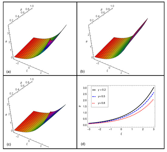
In Figure 1, we make a comparison between both the approximate solution (18) or (24) at $\wp =1$ using ADTM/VITM and the exact solution (25) to Equation (11). Moreover, the absolute error for this case is estimated at $t=0.1$, as demonstrated in Table 1. Almost perfect agreement between the two solutions is noted, which confirms the high accuracy and high efficiency of the used approximate methods (ADTM/VITM). On the other hand, the obtained approximations (18) or (24) are simulated numerically at different values of the fractional-order ℘, as shown in Figure 2. From the later figure, we can observe the effect of changing ℘ on the profile of the solutions. This graphical representation allows us to visually observe any changes in the shape, magnitude, or other properties of the solution as ℘ varies. These graphical discussions provide a visual representation of the solutions obtained using ADTM/VITM for Example 1 at different values of $\wp 1$. They help us to understand the impact of changing the fractional order on the behavior of the solution, allowing for a more comprehensive analysis of the problem.

Figure 1. In this figure, both the approximate solution (18) or (24) at $\gamma =\wp =1$ using ADTM/VITM and the exact solution (25) are considered for Example 1.

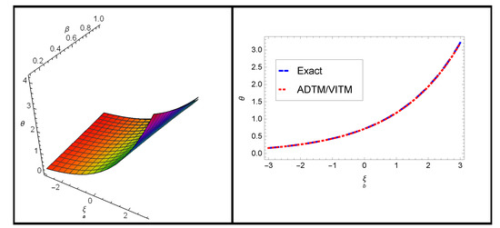
Table 1. Numerical values for both approximate and exact solutions for Example 1 and the absolute error.

x	ADTM/VITM	Exact Solution	Absolute Error
−1.0	0.567414	0.567839	0.000425389
−0.9	0.596506	0.596953	0.000447199
−0.8	0.627089	0.627559	0.000470128
−0.7	0.659241	0.659735	0.000494232
−0.6	0.693041	0.69356	0.000519572
−0.5	0.728574	0.72912	0.000546211
−0.4	0.765928	0.766503	0.000574215
−0.3	0.805198	0.805802	0.000603656
−0.2	0.846482	0.847116	0.000634606
−0.1	0.889882	0.890549	0.000667143
0.0	0.935507	0.936208	0.000701348
0.1	0.983471	0.984209	0.000737307
0.2	1.0339	1.03467	0.00077511
0.3	1.0869	1.08772	0.00081485
0.4	1.14263	1.14349	0.000856629
0.5	1.20121	1.20212	0.000900549

Figure 2. In this figure, both the approximate solution (18) or (24) using ADTM/VITM for Example 1 at different values of ℘ is considered: (a) $\wp =0.2$, (b) $\wp =0.5$ (c) $\wp =0.8$, and (d) two-dimensional plot for the cases (a–c) at $t=0.1$.

Example 2. 

Consider the following nonlinear FFWE [51]:

$$D_{ß}^{\wp }\theta -D_{\xi \xi ß}\theta +D_{\xi }\theta =\theta D_{\xi \xi \xi }\theta -\theta D_{\xi }\theta +3D_{\xi }\theta D_{\xi \xi }\theta ,ß>0,0<\wp \le 1,$$

(26)

with the initial condition

$$\theta (\xi ,0)={cosh}^2\left(\frac{\xi }{4}\right).$$

(27)

Applying the AT to (26), we obtain

$$\begin{array}{cc}\hfill \left(\frac{N(\wp )}{1-\wp +\wp {\varpi }^{-\wp }}\right)\left\{\mathcal{A}\left[\theta (\xi ,ß)\right]-\frac{1}{{\varpi }^2}\theta (\xi ,0)\right\}& \hfill =\mathcal{A}\left[D_{\xi \xi ß}\theta -D_{\xi }\theta +\theta D_{\xi \xi \xi }\theta -\theta D_{\xi }\theta +3D_{\xi }\theta D_{\xi \xi }\theta \right].\hfill \end{array}$$

Using the inverse of AT

$$\begin{array}{cc}\hfill \theta (\xi ,ß)=& \hfill {\mathcal{A}}^{-1}\left[\frac{\theta (\xi ,0)}{{\varpi }^2}-\left(\frac{1-\wp +\wp {\varpi }^{-\wp }}{N(\wp )}\right)\mathcal{A}\left\{D_{\xi \xi ß}\theta -D_{\xi }\theta +\theta D_{\xi \xi \xi }\theta -\theta D_{\xi }\theta +3D_{\xi }\theta D_{\xi \xi }\theta \right\}\right].\hfill \end{array}$$

Using the ADM procedure, we find

$${\theta }_0(\xi ,ß)={\mathcal{A}}^{-1}\left[\frac{\theta (\xi ,0)}{{\varpi }^2}\right]={\mathcal{A}}^{-1}\left[\frac{exp\left({cosh}^2\left(\frac{\xi }{4}\right)\right)}{{\varpi }^2}\right],$$

$${\theta }_0(\xi ,ß)={cosh}^2\left(\frac{\xi }{4}\right),$$

(28)

$$\begin{array}{cc}& \hfill \sum _{\varphi =0}^{\infty }{\theta }_{\varphi +1}(\xi ,ß)={\mathcal{A}}^{-1}\left[\left(\frac{1-\wp +\wp {\varpi }^{-\wp }}{N(\wp )}\right)\mathcal{A}\left[\sum _{\varphi =0}^{\infty }{\left(D_{\xi \xi ß}\theta \right)}_{\varphi }-\sum _{\varphi =0}^{\infty }{\left(D_{\xi }\theta \right)}_{\varphi }+\sum _{\varphi =0}^{\infty }{A}_{\varphi }-\sum _{\varphi =0}^{\infty }{B}_{\varphi }+3\sum _{\varphi =0}^{\infty }{C}_{\varphi }\right]\right],\varphi =0,1,2,\cdots \hfill \end{array}$$

for $\varphi =0$

$$\begin{array}{cc}\hfill {\theta }_1(\xi ,ß)& \hfill ={\mathcal{A}}^{-1}\left[\left(\frac{1-\wp +\wp {\varpi }^{-\wp }}{N(\wp )}\right)\mathcal{A}\left[D_{\xi \xi ß}{\theta }_0-D_{\xi }{\theta }_0+A_0-B_0+3C_0\right]\right]=-\frac{11}{32}sinh\left(\frac{\xi }{4}\right)\left((1-\wp )+\frac{\wp {ß}^{\wp }}{\mathsf{\Gamma }(\wp +1)}\right).\hfill \end{array}$$

(29)

for $\varphi =1$

$$\begin{array}{ll}{\theta }_2(\xi ,ß)=& {\mathcal{A}}^{-1}\left[\left(\frac{1-\wp +\wp {\varpi }^{-\wp }}{N(\wp )}\right)\mathcal{A}\left[D_{\xi \xi ß}{\theta }_1-D_{\xi }{\theta }_1+A_1-B_1+3C_1\right]\right],\\ {\theta }_2(\xi ,ß)=& -\frac{11}{28}sinh\left(\frac{\xi }{4}\right)\left((1-\wp )+\frac{\wp {ß}^{\wp }}{\mathsf{\Gamma }(\wp +1)}\right)+\frac{121}{1024}cosh\left(\frac{\xi }{4}\right)\left({(1-\wp )}^2+\frac{{\wp }^2{ß}^{2\wp }}{\mathsf{\Gamma }(2\wp +1)}+\frac{2(1-\wp )\wp {ß}^{\wp }}{\mathsf{\Gamma }(\wp +1)}\right),\end{array}$$

(30)

for $\varphi =2$

$$\begin{array}{ll}{\theta }_3(\xi ,ß)=& {\mathcal{A}}^{-1}\left[\left(\frac{1-\wp +\wp {\varpi }^{-\wp }}{N(\wp )}\right)\mathcal{A}\left[D_{\xi \xi ß}{\theta }_2-D_{\xi }{\theta }_2+A_2-B_2+3C_2\right]\right],\\ {\theta }_3(\xi ,ß)=& -\frac{11}{512}sinh\left(\frac{\xi }{4}\right)\left((1-\wp )+\frac{\wp {ß}^{\wp }}{\mathsf{\Gamma }(\wp +1)}\right)+\frac{121}{2048}cosh\left(\frac{\xi }{4}\right)\left({(1-\wp )}^2+\frac{{\wp }^2{ß}^{2\wp }}{\mathsf{\Gamma }(2\wp +1)}+\frac{2(1-\wp )\wp {ß}^{\wp }}{\mathsf{\Gamma }(\wp +1)}\right)\\ & -\frac{1331}{\mathrm{49,152}}sinh\left(\frac{\xi }{4}\right)\left\{{(1-\wp )}^3+\wp (1-\wp )(1+\wp +2{\wp }^2)\frac{{ß}^{\wp }}{\mathsf{\Gamma }(\wp +1)}+\frac{3{\wp }^2(1-\wp ){ß}^{2\wp }}{\mathsf{\Gamma }(2\wp +1)}+\frac{{\wp }^3\mathsf{\Gamma }(2\wp +1){ß}^{3\wp }}{\mathsf{\Gamma }(3\wp +1)}\right\},\end{array}$$

(31)

The MDM solution of example (2) reads

$$\theta (\xi ,ß)={\theta }_0(\xi ,ß)+{\theta }_1(\xi ,ß)+{\theta }_2(\xi ,ß)+{\theta }_3(\xi ,ß)+{\theta }_4(\xi ,ß)+\cdots ,$$

$$\begin{array}{ll}\theta (\xi ,ß)& ={cosh}^2\left(\frac{\xi }{4}\right)-\frac{11}{32}sinh\left(\frac{\xi }{4}\right)\left((1-\wp )+\frac{\wp {ß}^{\wp }}{\mathsf{\Gamma }(\wp +1)}\right)-\frac{11}{28}sinh\left(\frac{\xi }{4}\right)\left((1-\wp )+\frac{\wp {ß}^{\wp }}{\mathsf{\Gamma }(\wp +1)}\right)\\ & +\frac{121}{1024}cosh\left(\frac{\xi }{4}\right)\left({(1-\wp )}^2+\frac{{\wp }^2{ß}^{2\wp }}{\mathsf{\Gamma }(2\wp +1)}+\frac{2(1-\wp )\wp {ß}^{\wp }}{\mathsf{\Gamma }(\wp +1)}\right)-\frac{11}{512}sinh\left(\frac{\xi }{4}\right)\left((1-\wp )+\frac{\wp {ß}^{\wp }}{\mathsf{\Gamma }(\wp +1)}\right)\\ & +\frac{121}{2048}cosh\left(\frac{\xi }{4}\right)\left({(1-\wp )}^2+\frac{{\wp }^2{ß}^{2\wp }}{\mathsf{\Gamma }(2\wp +1)}+\frac{2(1-\wp )\wp {ß}^{\wp }}{\mathsf{\Gamma }(\wp +1)}\right)-\frac{1331}{\mathrm{49,152}}sinh\left(\frac{\xi }{4}\right)\{{(1-\wp )}^3\\ & +\wp (1-\wp )(1+\wp +2{\wp }^2)\frac{{ß}^{\wp }}{\mathsf{\Gamma }(\wp +1)}+\frac{3{\wp }^2(1-\wp ){ß}^{2\wp }}{\mathsf{\Gamma }(2\wp +1)}+\frac{{\wp }^3\mathsf{\Gamma }(2\wp +1){ß}^{3\wp }}{\mathsf{\Gamma }(3\wp +1)}\}\cdots .\end{array}$$

(32)

To obtain an analytical solution, the variational method can be employed.

We can obtain the iteration formulas for Equation (26), as follows:

$$\begin{array}{cc}\hfill & \hfill {\theta }_{\varphi +1}(\xi ,ß)={\theta }_j(\xi ,ß)-{\mathcal{A}}^{-1}\left[\left(\frac{1-\wp +\wp {\varpi }^{-\wp }}{N(\wp )}\right)\mathcal{A}\left\{D_{\xi \xi ß}{\theta }_{\varphi }+D_{\xi }{\theta }_{\varphi }-{\theta }_{\varphi }{D}_{\xi \xi \xi }{\theta }_{\varphi }+{\theta }_{\varphi }{D}_{\xi }{\theta }_{\varphi }-3D_{\xi }{\theta }_{\varphi }{D}_{\xi \xi }{\theta }_{\varphi }\right\}\right],\hfill \end{array}$$

(33)

with

$$\begin{array}{c}\hfill {\theta }_0(\xi ,ß)={cosh}^2\left(\frac{\xi }{4}\right).\end{array}$$

(34)

For $\varphi =0,1,2,\cdots$

$$\begin{array}{ll}{\theta }_1(\xi ,ß)& ={\theta }_0(\xi ,ß)-{\mathcal{A}}^{-1}\left[\left(\frac{1-\wp +\wp {\varpi }^{-\wp }}{N(\wp )}\right)\mathcal{A}\left\{D_{\xi \xi ß}{\theta }_0+D_{\xi }{\theta }_0-{\theta }_0{D}_{\xi \xi \xi }{\theta }_0+{\theta }_0{D}_{\xi }{\theta }_0-3D_{\xi }{\theta }_0{D}_{\xi \xi }{\theta }_0\right\}\right],\\ {\theta }_1(\xi ,ß)& ={cosh}^2\left(\frac{\xi }{4}\right)-\frac{11}{32}sinh\left(\frac{\xi }{4}\right)\left((1-\wp )+\frac{\wp {ß}^{\wp }}{\mathsf{\Gamma }(\wp +1)}\right),\end{array}$$

(35)

$$\begin{array}{ll}{\theta }_2(\xi ,ß)& ={\theta }_1(\xi ,ß)-{\mathcal{A}}^{-1}\left[\left(\frac{1-\wp +\wp {\varpi }^{-\wp }}{N(\wp )}\right)\mathcal{A}\left\{D_{\xi \xi ß}{\theta }_1+D_{\xi }{\theta }_1-{\theta }_1{D}_{\xi \xi \xi }{\theta }_1+{\theta }_1{D}_{\xi }{\theta }_1-3D_{\xi }{\theta }_1{D}_{\xi \xi }{\theta }_1\right\}\right],\\ {\theta }_2(\xi ,ß)& ={cosh}^2\left(\frac{\xi }{4}\right)-\frac{11}{32}sinh\left(\frac{\xi }{4}\right)\left((1-\wp )+\frac{\wp {ß}^{\wp }}{\mathsf{\Gamma }(\wp +1)}\right)-\frac{11}{28}sinh\left(\frac{\xi }{4}\right)\left((1-\wp )+\frac{\wp {ß}^{\wp }}{\mathsf{\Gamma }(\wp +1)}\right)\\ & +\frac{121}{1024}cosh\left(\frac{\xi }{4}\right)\left({(1-\wp )}^2+\frac{{\wp }^2{ß}^{2\wp }}{\mathsf{\Gamma }(2\wp +1)}+\frac{2(1-\wp )\wp {ß}^{\wp }}{\mathsf{\Gamma }(\wp +1)}\right),\end{array}$$

(36)

$$\begin{array}{ll}{\theta }_3(\xi ,ß)=& {\theta }_2(\xi ,ß)-{\mathcal{A}}^{-1}\left[\left(\frac{1-\wp +\wp {\varpi }^{-\wp }}{N(\wp )}\right)\mathcal{A}\left\{D_{\xi \xi ß}{\theta }_2+D_{\xi }{\theta }_2-{\theta }_2{D}_{\xi \xi \xi }{\theta }_2+{\theta }_2{D}_{\xi }{\theta }_2-3D_{\xi }{\theta }_2{D}_{\xi \xi }{\theta }_2\right\}\right],\\ {\theta }_3(\xi ,ß)=& {cosh}^2\left(\frac{\xi }{4}\right)-\frac{11}{32}sinh\left(\frac{\xi }{4}\right)\left((1-\wp )+\frac{\wp {ß}^{\wp }}{\mathsf{\Gamma }(\wp +1)}\right)-\frac{11}{28}sinh\left(\frac{\xi }{4}\right)\left((1-\wp )+\frac{\wp {ß}^{\wp }}{\mathsf{\Gamma }(\wp +1)}\right)\\ & +\frac{121}{1024}cosh\left(\frac{\xi }{4}\right)\left({(1-\wp )}^2+\frac{{\wp }^2{ß}^{2\wp }}{\mathsf{\Gamma }(2\wp +1)}+\frac{2(1-\wp )\wp {ß}^{\wp }}{\mathsf{\Gamma }(\wp +1)}\right)-\frac{11}{512}sinh\left(\frac{\xi }{4}\right)\left((1-\wp )+\frac{\wp {ß}^{\wp }}{\mathsf{\Gamma }(\wp +1)}\right)\\ & +\frac{121}{2048}cosh\left(\frac{\xi }{4}\right)\left({(1-\wp )}^2+\frac{{\wp }^2{ß}^{2\wp }}{\mathsf{\Gamma }(2\wp +1)}+\frac{2(1-\wp )\wp {ß}^{\wp }}{\mathsf{\Gamma }(\wp +1)}\right)-\frac{1331}{\mathrm{49,152}}sinh\left(\frac{\xi }{4}\right)\{{(1-\wp )}^3+\\ & \wp (1-\wp )(1+\wp +2{\wp }^2)\frac{{ß}^{\wp }}{\mathsf{\Gamma }(\wp +1)}+\frac{3{\wp }^2(1-\wp ){ß}^{2\wp }}{\mathsf{\Gamma }(2\wp +1)}+\frac{{\wp }^3\mathsf{\Gamma }(2\wp +1){ß}^{3\wp }}{\mathsf{\Gamma }(3\wp +1)}\},\end{array}$$

(37)

$$\begin{array}{ll}\theta (\xi ,ß)=& {cosh}^2\left(\frac{\xi }{4}\right)-\frac{11}{32}sinh\left(\frac{\xi }{4}\right)\left((1-\wp )+\frac{\wp {ß}^{\wp }}{\mathsf{\Gamma }(\wp +1)}\right)-\frac{11}{28}sinh\left(\frac{\xi }{4}\right)\left((1-\wp )+\frac{\wp {ß}^{\wp }}{\mathsf{\Gamma }(\wp +1)}\right)\\ & +\frac{121}{1024}cosh\left(\frac{\xi }{4}\right)\left({(1-\wp )}^2+\frac{{\wp }^2{ß}^{2\wp }}{\mathsf{\Gamma }(2\wp +1)}+\frac{2(1-\wp )\wp {ß}^{\wp }}{\mathsf{\Gamma }(\wp +1)}\right)-\frac{11}{512}sinh\left(\frac{\xi }{4}\right)\left((1-\wp )+\frac{\wp {ß}^{\wp }}{\mathsf{\Gamma }(\wp +1)}\right)\\ & +\frac{121}{2048}cosh\left(\frac{\xi }{4}\right)\left({(1-\wp )}^2+\frac{{\wp }^2{ß}^{2\wp }}{\mathsf{\Gamma }(2\wp +1)}+\frac{2(1-\wp )\wp {ß}^{\wp }}{\mathsf{\Gamma }(\wp +1)}\right)-\frac{1331}{\mathrm{49,152}}sinh\left(\frac{\xi }{4}\right)\{{(1-\wp )}^3+\\ & \wp (1-\wp )(1+\wp +2{\wp }^2)\frac{{ß}^{\wp }}{\mathsf{\Gamma }(\wp +1)}+\frac{3{\wp }^2(1-\wp ){ß}^{2\wp }}{\mathsf{\Gamma }(2\wp +1)}+\frac{{\wp }^3\mathsf{\Gamma }(2\wp +1){ß}^{3\wp }}{\mathsf{\Gamma }(3\wp +1)}\}+\cdots .\end{array}$$

(38)

We put $\wp =1$; then, the series solution is given as

$$\begin{array}{ll}\theta (\xi ,ß)=& {cosh}^2\left(\frac{\xi }{4}\right)-\frac{11}{32}sinh\left(\frac{\xi }{4}\right)ß-\frac{11}{28}sinh\left(\frac{\xi }{4}\right)ß\\ & +\frac{121}{1024}cosh\left(\frac{\xi }{4}\right)\frac{{\wp }^2}{2}-\frac{11}{512}sinh\left(\frac{\xi }{4}\right)\wp \\ & +\frac{121}{2048}cosh\left(\frac{\xi }{4}\right)\frac{{\wp }^2}{2}-\frac{1331}{\mathrm{49,152}}sinh\left(\frac{\xi }{4}\right)\frac{{\wp }^3}{3}+\cdots .\end{array}$$

(39)

The exact result of Equation (26) at $\wp =1$ reads

$$\begin{array}{c}\hfill \theta (\xi ,ß)={cosh}^2\left(\frac{\xi }{4}-\frac{11ß}{24}\right).\end{array}$$

(40)

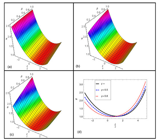
In Figure 3, a comparison between both the approximate solution (32) or (38) at $\wp =1$ using ADTM/VITM and the exact solution (40) to Equation (26) is presented. Further, the absolute error for this case is estimated at $t=0.1$, as illustrated in Table 2. It is noted from the comparison results that the two solutions are compatible to a large degree, which enhances the accuracy and efficiency of the used numerical techniques (ADTM/VITM). Additionally, the obtained approximations (32) or (38) are displayed in Figure 4 at different values of the fractional-order ℘. This graphical representation allows us to visually observe any changes in the shape, magnitude, or other properties of the solution as ℘ varies. These graphical discussions provide a visual representation of the solutions obtained using ADTM/VITM for Example 2 at different values of ℘. These figures demonstrate how the wavepacket evolves and interacts within the dispersive medium according to the Fornberg–Whitham equation. Comparing this figure with the previous one at $\wp =1$, noticeable changes in the wavepacket’s behavior can be observed. The alterations might include variations in amplitude, shape, and propagation speed. These changes indicate the influence of the fractional order on the dynamics of the wavepacket. By examining both Figure 3 and Figure 4, it becomes evident that altering the fractional order affects the characteristics of the solutions to Equation (26). The plots provide graphical insights into how changes in the fractional order parameter influence the wavepacket’s behavior, allowing for a better understanding of the physical significance of the equation.

Figure 3. In this figure, both the approximate solution (32) or (38) at $\wp =1$ using ADTM/VITM and the exact solution (40) are considered for Example 2.

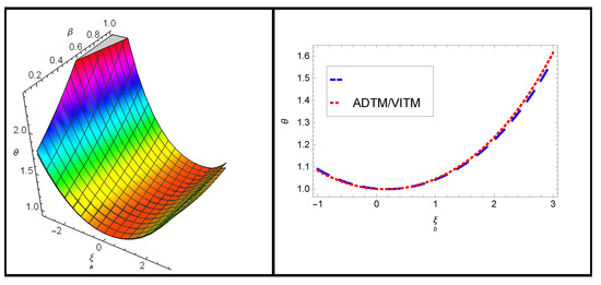
Table 2. Numerical values of both approximate and exact solutions for Example 2 and the absolute error.

x	ADTM/VITM	Exact Solution	Absolute Error
0.0	1.0021	1.00089	0.00121594
0.1	1.00043	0.999616	0.000818105
0.2	1.00002	0.999597	0.000420427
0.3	1.00085	1.00083	0.0000183526
0.4	1.00294	1.00333	0.000392684
0.5	1.00628	1.0071	0.000817276
0.6	1.01089	1.01215	0.00126006
0.7	1.01678	1.0185	0.00172572
0.8	1.02396	1.02618	0.00221902
0.9	1.03245	1.03519	0.0027448
1.0	1.04227	1.04557	0.003308

Figure 4. In this figure, both the approximate solution (32) or (38) using ADTM/VITM for Example 2 at different values of ℘ is considered: (a) $\wp =0.2$, (b) $\wp =0.5$ (c) $\wp =0.8$, and (d) two-dimensional plot for the cases (a–c) at $t=0.1$.

5. Conclusions

In summing up, this study has presented a comprehensive comparison between the Adomian decomposition method (ADM) and the variational iteration method (VIM) for solving the fractional Fornberg–Whitham equation (FFWE) in the sense of the Aboodh transformation. Both methods have demonstrated their effectiveness and accuracy in solving this complex nonlinear fractional partial differential equation (FPDE). The ADM and VIM were employed to obtain approximate solutions of the FFWE, taking into account their inherent advantages and limitations. The ADM, a semi-analytical method, was shown to provide a systematic approach to constructing the solution in the form of a convergent series, while the VIM, an iterative method, provided a more straightforward and simpler approach for obtaining approximate solutions. A thorough analysis of the numerical results revealed that both methods have the potential to deliver accurate and reliable solutions to the FFWE. However, the choice of the most appropriate method may depend on the specific problem at hand, the computational resources, and the desired level of accuracy. Future research could focus on extending the application of these methods to other types of FPDEs, as well as exploring the combination of these methods with other numerical or analytical techniques to enhance their efficiency and accuracy. Furthermore, the implementation of these methods in high-performance computing environments could be investigated to tackle more complex problems and improve computational efficiency.

References

- Johnson, R.S. Fornberg-Whitham equation. In Encyclopedia of Mathematics and Its Applications; Cambridge University Press: Cambridge, UK, 1997; Volume 60, pp. 35–37. [Google Scholar]
- Choi, W.; Camassa, R. Fully nonlinear internal waves in a two-fluid system. J. Fluid Mech. 2007, 581, 369–380. [Google Scholar] [CrossRef]
- He, H.M.; Peng, J.G.; Li, H.Y. Iterative approximation of fixed point problems and variational inequality problems on Hadamard manifolds. UPB Bull. Ser. A 2022, 84, 25–36. [Google Scholar]
- Xie, X.; Huang, L.; Marson, S.M.; Wei, G. Emergency response process for sudden rainstorm and flooding: Scenario deduction and Bayesian network analysis using evidence theory and knowledge meta-theory. Nat. Hazards 2023, 117, 3307–3329. [Google Scholar] [CrossRef]
- Jin, H.Y.; Wang, Z.A. Global stabilization of the full attraction-repulsion Keller-Segel system. Discret. Contin. Dyn. Syst. Ser. A 2020, 40, 3509–3527. [Google Scholar] [CrossRef]
- Guo, C.; Hu, J. Fixed-Time Stabilization of High-Order Uncertain Nonlinear Systems: Output Feedback Control Design and Settling Time Analysis. J. Syst. Sci. Complex. 2023. [Google Scholar] [CrossRef]
- Lyu, W.; Wang, Z. Global classical solutions for a class of reaction-diffusion system with density-suppressed motility. Electron. Res. Arch. 2022, 30, 995–1015. [Google Scholar] [CrossRef]
- Shah, N.A.; Hamed, Y.S.; Abualnaja, K.M.; Chung, J.D.; Khan, A. A comparative analysis of fractional-order kaup-kupershmidt equation within different operators. Symmetry 2022, 14, 986. [Google Scholar] [CrossRef]
- Ostrovsky, L.A.; Pelinovsky, E.N.; Shrira, V.I. Rogue waves in nonlinear dispersive media: Physical mechanisms, models, and applications. Phys. Rep. 2008, 443, 1–53. [Google Scholar]
- Stolen, R.H.; Gordon, J.P. Self-phase-modulation and small-scale filaments in nonlinear fibers. Opt. Lett. 1982, 7, 28–33. [Google Scholar]
- Fornberg, B.; Whitham, G.B. A numerical and theoretical study of certain nonlinear wave phenomena. Philos. Trans. R. Soc. A Math. Phys. Eng. Sci. 1978, 289, 373–404. [Google Scholar]
- Fornberg, B.; Whitham, G.B. A numerical and theoretical study of certain nonlinear wave phenomena. II. Nonlinear geometrical optics. Philos. Trans. R. Soc. A Math. Phys. Eng. Sci. 1979, 292, 385–409. [Google Scholar]
- Fornberg, B. Numerical solution of the Fornberg-Whitham equation. J. Comput. Phys. 1980, 36, 362–381. [Google Scholar]
- Zayed, E.M.; Rahman, H.M.A. On using the modified variational iteration method for solving the nonlinear coupled equations in the mathematical physics. Ric. Mat. 2010, 59, 137–159. [Google Scholar] [CrossRef]
- Zayed, E.M.E.; Nofal, T.A.; Gepreel, K.A. The travelling wave solutions for non-linear initial-value problems using the homotopy perturbation method. Int. J. Control. 2009, 88, 617–634. [Google Scholar] [CrossRef]
- Zhang, K.; Alshehry, A.S.; Aljahdaly, N.H.; Shah, N.A.; Ali, M.R. Efficient computational approaches for fractional-order Degasperis-Procesi and Camassa-Holm equations. Results Phys. 2023, 50, 106549. [Google Scholar] [CrossRef]
- Abu Hammad, M. Conformable Fractional Martingales and Some Convergence Theorems. Mathematics 2021, 10, 6. [Google Scholar] [CrossRef]
- Dahmani, Z.; Anber, A.; Gouari, Y.; Kaid, M.; Jebril, I. Extension of a Method for Solving Nonlinear Evolution Equations Via Conformable Fractional Approach. In Proceedings of the 2021 International Conference on Information Technology (ICIT 2021), Amman, Jordan, 14–15 July 2021; pp. 38–42. [Google Scholar]
- Batiha, I.M.; Oudetallah, J.; Ouannas, A.; Al-Nana, A.A.; Jebril, I.H. Tuning the fractional-order pid-controller for blood glucose level of diabetic patients. Int. J. Adv. Soft Comput. Its Appl. 2021, 13, 1–10. [Google Scholar]
- Deng, W.; Li, C. Existence and uniqueness of solutions for the fractional Fornberg-Whitham equation with initial and boundary conditions. Appl. Math. Lett. 2010, 23, 937–942. [Google Scholar] [CrossRef]
- Liu, F.; Anh, V. Well-posedness of the fractional Fornberg-Whitham equation with different types of boundary conditions. Comput. Math. Appl. 2011, 62, 1295–1303. [Google Scholar]
- Zhang, H.; Deng, W. A finite difference scheme for the fractional Fornberg-Whitham equation. J. Comput. Appl. Math. 2013, 239, 12–23. [Google Scholar]
- Liu, F.; Li, X.; Zhao, X. A finite volume method for the fractional Fornberg-Whitham equation. J. Comput. Phys. 2015, 295, 336–353. [Google Scholar]
- Li, C.; Deng, W.; Zhu, M. A spectral method for the fractional Fornberg-Whitham equation. Numer. Algorithms 2018, 79, 377–392. [Google Scholar]
- Hu, X.; Li, C.; Deng, W. Fractional Fornberg-Whitham equation for the dynamics of stock prices. J. Appl. Math. Comput. 2016, 50, 601–612. [Google Scholar]
- Wang, Y.; Zhang, C.; Song, W. Image denoising using the fractional Fornberg-Whitham equation. J. Comput. Appl. Math. 2015, 279, 152–161. [Google Scholar]
- Zhang, J.; Xie, J.; Shi, W.; Huo, Y.; Ren, Z.; He, D. Resonance and bifurcation of fractional quintic Mathieu-Duffing system. Chaos Interdiscip. J. Nonlinear Sci. 2023, 33, 23131. [Google Scholar] [CrossRef] [PubMed]
- Qi, M.; Cui, S.; Chang, X.; Xu, Y.; Meng, H.; Wang, Y.; Arif, M. Multi-region Nonuniform Brightness Correction Algorithm Based on L-Channel Gamma Transform. Secur. Commun. Netw. 2022, 2022, 2675950. [Google Scholar] [CrossRef]
- Zhu, H.; Xue, M.; Wang, Y.; Yuan, G.; Li, X. Fast Visual Tracking with Siamese Oriented Region Proposal Network. IEEE Signal Process. Lett. 2022, 29, 1437. [Google Scholar] [CrossRef]
- Guo, F.; Zhou, W.; Lu, Q.; Zhang, C. Path extension similarity link prediction method based on matrix algebra in directed networks. Comput. Commun. 2022, 187, 83–92. [Google Scholar] [CrossRef]
- Song, J.; Mingotti, A.; Zhang, J.; Peretto, L.; Wen, H. Accurate Damping Factor and Frequency Estimation for Damped Real-Valued Sinusoidal Signals. IEEE Trans. Instrum. Meas. 2022, 71, 6503504. [Google Scholar] [CrossRef]
- He, J.H. variational iteration method-a kind of nonlinear analytical technique: Some examples. Int. J. Non-Linear Mech. 2007, 34, 699–708. [Google Scholar] [CrossRef]
- He, J.H. variational iteration method for autonomous ordinary differential systems. Appl. Math. Comput. 2010, 217, 869–877. [Google Scholar] [CrossRef]
- Khader, M.M.; Hashim, I. Numerical methods for solving fractional differential equations: A comparative study. J. Comput. Appl. Math. 2016, 305, 195–210. [Google Scholar]
- Gao, G.H.; Li, X.Z.; He, J.H. Chaos in the fractional order Chen system and its control. Chaos Solitons Fractals 2004, 22, 549–554. [Google Scholar] [CrossRef]
- Hu, Y.; Sun, Z. Variational iteration transform method for solving the coupled Burgers’ equations with time-fractional derivatives. Appl. Math. Comput. 2017, 303, 132–141. [Google Scholar]
- Shah, N.A.; Alyousef, H.A.; El-Tantawy, S.A.; Chung, J.D. Analytical investigation of fractional-order Korteweg-De-Vries-type equations under Atangana-Baleanu-Caputo operator: Modeling nonlinear waves in a plasma and fluid. Symmetry 2022, 14, 739. [Google Scholar] [CrossRef]
- Xu, L.; Cao, X. The variational iteration transform method for solving the time-space fractional Fisher equation. Appl. Math. Comput. 2017, 305, 188–194. [Google Scholar]
- Wang, J.; Tian, J.; Zhang, X.; Yang, B.; Liu, S.; Yin, L.; Zheng, W. Control of Time Delay Force Feedback Teleoperation System with Finite Time Convergence. Front. Neurorobot. 2022, 16, 877069. [Google Scholar] [CrossRef]
- Jafari, H.; Seifi, S. Analytical solution of a nonlinear differential equation using the Variational Iteration Transform Method. J. Math. Anal. Appl. 2017, 446, 1261–1275. [Google Scholar]
- Adomian, G. A review of the decomposition method and some recent results for nonlinear equations. Math. Comput. Model. 1988, 13, 17–43. [Google Scholar] [CrossRef]
- Wazwaz, A.M. A First Course in Integral Equations; World Scientific: Singapore, 2002. [Google Scholar]
- Momani, S.; Odibat, Z. Analytical solution of a time-fractional Navier-Stokes equation by Adomian decomposition method. Appl. Math. Comput. 2007, 177, 488–494. [Google Scholar] [CrossRef]
- Abbasbandy, S.; Shirzadi, A. Application of the Adomian decomposition method for solving a system of nonlinear fractional differential equations. Commun. Nonlinear Sci. Numer. Simul. 2011, 16, 210–219. [Google Scholar]
- Eftekhari, G.; Alhuthali, M.S. Solving fractional partial differential equations using the Adomian decomposition method. J. Comput. Appl. Math. 2018, 339, 318–328. [Google Scholar]
- Cakir, M.; Arslan, D. The Adomian Decomposition Method and the Differential Transform Method for Numerical Solution of Multi-Pantograph Delay Differential Equations. Appl. Math. 2015, 6, 1332. [Google Scholar] [CrossRef]
- Bhrawy, A.H.; Alofi, A.S. Solving nonlinear differential equations by the modified Adomian decomposition method with application to wave equation. Results Phys. 2021, 26, 104708. [Google Scholar]
- Benattia, M.E.; Belghaba, K. Application of the Aboodh transform for solving fractional delay differential equations. Univers. J. Math. Appl. 2020, 3, 93–101. [Google Scholar] [CrossRef]
- Awuya, M.A.; Subasi, D. Aboodh transform iterative method for solving fractional partial differential equation with Mittag-Leffler Kernel. Symmetry 2021, 13, 2055. [Google Scholar] [CrossRef]
- Gupta, P.K.; Singh, M. Homotopy perturbation method for fractional Fornberg-Whitham equation. Comput. Math. Appl. 2011, 61, 250–254. [Google Scholar] [CrossRef]
- Abidi, F.; Omrani, K. Numerical solutions for the nonlinear Fornberg-Whitham equation by He’s methods. Int. J. Mod. Phys. B 2011, 25, 4721–4732. [Google Scholar] [CrossRef]
Disclaimer/Publisher’s Note: The statements, opinions and data contained in all publications are solely those of the individual author(s) and contributor(s) and not of MDPI and/or the editor(s). MDPI and/or the editor(s) disclaim responsibility for any injury to people or property resulting from any ideas, methods, instructions or products referred to in the content. |
© 2023 by the authors. Licensee MDPI, Basel, Switzerland. This article is an open access article distributed under the terms and conditions of the Creative Commons Attribution (CC BY) license (https://creativecommons.org/licenses/by/4.0/).