Embed-Solitons in the Context of Functions of Symmetric Hyperbolic Fibonacci

Abstract

In this article, we discuss the findings of new developments in a class of new triangular functions that blend the quantity functions of the traditional triangular. Considering the significant role played by the triangular functions in applied mathematics, physics, and engineering, it is conceivable to predict that the theory of new triangular functions will provide us with additional interpretations and discoveries in mathematics and physics. The solutions which consider variable separation based on arbitrary functions are constructed to the (3+1)-dimensional Burgers model by presenting the Fibonacci Riccati technique and the linearly independent variable separation approach. This technique’s fundamental concept is to describe the solution of the Burgers model as a polynomial in the Riccati Equation solution that satisfies the symmetrical hyperbolic and triangular Fibonacci functions. Depending on the choice of suitable functions for variable separation, an abundance of new localized solutions were obtained. Moreover, examples such as embedded solitons, rectangle-solitons, plateau-type ring solitons, taper-like solitons, and their interactions with each other, following the symmetrical hyperbolic and triangular Fibonacci functions, as well as the golden mean, could be explored.

1. Introduction

Scott Russell was the first to notice the solitary waves that De-Vries and Korteweg would later use in their KdV equation. Between now and then, the authors of [1,2] may use the nonlinear Schrodinger (NLS) equation [3] to explain the standing force or the solitary wave of the non-propagating type, termed a breather. The NLS equation was created by the authors of [4,5]. However, the literature on solitary waves of the non-propagating type in higher dimensions, particularly in systems with the (2+1)-dimensional non-linearity, is deficient despite several theoretical and practical works [6,7]. Recently, there has been a formula that works for everyone [7].

$$\mathit{u}\mathbf{=}\frac{\mathbf{2}\mathbf{(}{\mathit{a}}_{\mathbf{2}}{\mathit{a}}_{\mathbf{1}}\mathbf{-}{\mathit{a}}_{\mathbf{3}}{\mathit{a}}_{\mathbf{0}}\mathbf{)}{\mathit{q}}_{\mathit{y}}{\mathit{p}}_{\mathit{x}}}{\mathbf{(}{\mathit{a}}_{\mathbf{0}}\mathbf{+}{\mathit{a}}_{\mathbf{1}}\mathit{p}\mathbf{+}{\mathit{a}}_{\mathbf{2}}\mathit{q}\mathbf{+}{\mathit{a}}_{\mathbf{3}}\mathit{p}\mathit{q}{\mathbf{)}}^{\mathbf{2}}}$$

(1)

Equation (1) fits the appropriate potential or physical fields for an enormous kind of (2+1)-dimensional, naturally stimulating nonlinear equations and systems. Examples include the dispersive long wave (DLW) systems, Davey–Stewartson (DS), Broer–Kaup–Kupershimidt (BKK) system, asymmetric DS, Nizhnik–Novikov–Veselov (NVV), asymmetric NNV system, generalized NNV equation, Maccari system, long wave-short wave interaction model, general (N+M)-component AKNS system, (2+1)-dimensional Ablowitz–Kaup–Newell–Segur (AKNS) system, (2+1)-dimensional KdV equation, as well as (2+1)-dimensional sine-Gordon Equation [6,7,8], depending on the technique of multilinear variable separation. In (1), the function $\mathit{p}\equiv \mathit{p}(\mathit{x},\mathit{t})$ represents the $\{\mathit{x},\mathit{t}\}$ arbitrary function. The function $\mathit{q}\equiv \mathit{q}(\mathit{y},\mathit{t})$ is possibly the arbitrary solution of a Riccati Equation or the arbitrary function of $\{\mathit{y},\mathit{t}\}$, whereas ${\mathit{a}}_{\mathbf{0}},{\mathit{a}}_{\mathbf{1}},{\mathit{a}}_{\mathbf{2}}$, and ${\mathit{a}}_{\mathbf{3}}$ are given as constants. Using Equation (1), we can construct quite rich localized excitements, e.g., dromions, lumps, ring solitons, foldons, compactons, peakons, as well as chaotic and fractal patterns. In addition, the non-localized ones, including the doubly periodic waves and solitons, are attained. Newly discovered interactions between the same and distinct types of soliton excitations are also emphasized. Localized excitement, on the other hand, can be more thrilling. For example, embed-solitons and [9,10] taper-like solitons can be created in a higher dimensional [11]. This subject is intriguing to consider. The Burgers model, a well-known (3+1)-dimensional model, must be considered in order to resolve this problem [12].

$$\begin{gathered} {\mathit{u}}_{\mathit{t}}\mathbf{=}\mathbf{2}\mathit{u}{\mathit{u}}_{\mathit{y}}\mathbf{+}\mathbf{2}\mathit{v}{\mathit{u}}_{\mathit{x}}\mathbf{+}\mathbf{2}\mathit{w}{\mathit{u}}_{\mathit{z}}\mathbf{+}{\mathit{u}}_{\mathit{x}\mathit{x}}\mathbf{+}{\mathit{u}}_{\mathit{y}\mathit{y}}\mathbf{+}{\mathit{u}}_{\mathit{z}\mathit{z}}\mathbf{,} \\ {\mathit{u}}_{\mathit{x}}\mathbf{-}{\mathit{v}}_{\mathit{y}}\mathbf{=}\mathbf{0}\mathbf{,}{\mathit{u}}_{\mathit{z}}\mathbf{-}{\mathit{w}}_{\mathit{y}}\mathbf{=}\mathbf{0}\mathbf{,} \end{gathered}$$

(2)

which is a general form of the Burgers model in (3+1)-dimensions. When u becomes z-independent (putting z = x, w = u), system (2) declines to the Burgers model in the (2+1)-dimensional, a result of the generalized integrability of Painleve categorization. System (2) was demonstrated to be a resolvable multilinear variable separation technique. When u becomes independent of z and y, system (2) is an ordinary Burgers model of the (1+1)-dimensional applicable in several fields. Based on the invertible deformation of the Equation of thermal conductivity, another potential form of system (2) is derived. System (2) is explored through the multilinear variable separation technique. The rest of this manuscript discusses exact solutions with intriguing localized excitements via the Fibonacci Riccati approach. In this context, it should be noted that in the majority of previous research, equations with many variables are converted into equations with one variable, using travelling waves. This technique converts PDEs into a set of algebraic equations whose solutions can be found easily, however here in this manuscript, we attempt to find solutions. In general, to simplify the solution, the connection between the Fibonacci Riccati approach and the linear variable separation is used.

According to the Fibonacci Riccati system cited in the study results, solitons, embed-solitons, and their development features stimulate localized coherent excitations [12,13]. Nature’s two most important mathematical constants, π and e, significantly influence physics and mathematics [14]. Their significance is because they “create” the most essential “primary functions”: cosine, sin, hyperbolic, exponential, and logarithmic functions (the e-numbers) [15]. These functions [16] are critical to the study of physics and mathematics. For example, in cosmology and geometry, classical hyperbolic functions play a significant role [17]. The golden ratio, golden section, golden mean, and golden proportion are all mathematical constants that profoundly influence the formation of life systems [18,19]. However, the importance of this mathematical constant [20,21] in current mathematics and mathematical education may be degraded. Esoteric symbology strongly connects to the golden section (platonic solid, pentagonal star, pentagram, etc.). Unfortunately, modern science and education have denigrated the golden portion [22]. In stark contrast, a new viewpoint on the golden section’s Lucas and Fibonacci ratio’s is emerging. Scientific discoveries depending on the golden season have had a significant impact on the discoveries of contemporary science [23]. Human research is on the verge of discovering a very complex idea, such as the notion of harmony depending on the golden season [24,25]. In contrast to the chaos theory, the universe’s structure was intended by this concept [26]. One of the geometrical problems Euclid discusses in his writings is called “the difficulty of devising the line segment into its two extremes [27]; it is sometimes referred to as the difficulty of the golden section [28,29,30].

Solving this problem decreases the following Equation of algebraic type ${\mathit{x}}^{\mathbf{2}}\mathbf{=}\mathit{x}\mathbf{+}\mathbf{1}$. One of the roots of this Equation is $\mathit{\alpha }\mathbf{=}\mathbf{(}\mathbf{1}\mathbf{+}\sqrt{\mathbf{5}}\mathbf{)}\mathbf{/}\mathbf{2}$, representing the golden ratio, golden proportion, or golden mean. The works done by the authors of [30,31] promote the applications of the golden mean in applied mathematics and modern physics.

El Naschie [32] examined the vital role given by the golden mean in quantum physics and concluded that the concept of a space-time Cantorian, with its physical and complicated mathematics, should be adopted. Moreover, the implication of this synthesized the findings of topological quantum, geometrical quantum, as well as Rossler’s endophysics that deploy the concepts of the stochastic mechanism by Nelson [33,34]. According to Vladimirov, El-Naschie, Shechtman, Mauldin, Williams, and Butusov, the golden section is an integral part of modern physics and applied mathematics. Abdel-Salam [35] used the symmetrical Lucas functions to solve the Riccati Equation and obtain some structures of double periodic, periodic waves, and evolutional behaviors to the system of the DLW in (2+1)-dimension [36].

Recent research in applied mathematics and its related fields has led to significant advancements in our understanding of complex systems. For instance, Jin, Wang, and Wu [37] investigated the global dynamics of a three-species spatial food chain model, while Ping Liu, Junping Shi, and Zhi-An Wang [38] explored the pattern formation of the attraction-repulsion Keller-Segel system. Moreover, global stabilization of the full attraction-repulsion Keller-Segel system was studied by Jin and Wang [39]. Li et al. [40] developed an H∞ consensus for multiagent-based supply chain systems under switching topology and uncertain demands. In the field of finance, Li and Sun [41] proposed a stock intelligent investment strategy based on a support vector machine parameter optimization algorithm. Shao et al. [42] developed a linear AC unit commitment formulation using a data-driven linear power flow model in the context of electrical power and energy systems. These studies highlight the importance of mathematical modeling and its applications in addressing real-world challenges. Cai et al. [43] investigated the general formula of multiple non-degenerate soliton solutions for the Manakov system by the Kadomtsev–Petviashvili hierarchy reduction. Liu et al. in [44] discuss the localised nonlinear wave interaction in the generalised Kadomtsev-Petviashvili Equation using the Hirota bilinear scheme and τ-function formalism. Liu et al. in [45] proposed the nonlinear wave structures of the variable-coefficient (2+1)-dimensional Korteweg–de Vries system, using soliton solutions which were obtained via Hirota’s bilinear method. Refs. [46,47] discussed the optical solitons of the extended Gerdjikov-Ivanov equation in DWDM system, solitons and other solutions to Complex-Valued Klein-Gordon equation in ϕ-4 field theory. Zhu and Zheng [48] investigated the embed-Solitons of (3+1)-dimensional Burgers System. Abdel-Salam [49] studied the quasi-periodic structures on symmetrical lucas Function of (2+1)-dimensional modified dispersive water-wave system.

The following sections take this structure: Section 2 reviews the symmetrical Lucas functions and introduces the symmetrical triangular Fibonacci functions and their characteristics. The Fibonacci Riccati (FR) method for NLPDEs is represented in Section 3. In the last two sections, the FR system is applied to the (3+1)-dimensional Burgers system, and some novel localized excitations are discussed. Finally, we conclude the paper and provide concluding remarks.

2. The Tariffs and Characteristics of the Triangular Fibonacci Symmetrical Functions

The authors in [50,51] describe the development of a unique category of hyperbolic symmetrical functions that combines the features of classical hyperbolic functions with the recurrent Lucas and Fibonacci designation. The hyperbolic functions defined by Lucas and Fibonacci transform the Fibonacci theory into one that is “permanent”. Each item of the Lucas functions and hyperbolic Fibonacci comprises a unique analog in the paradigm of numbers given by Fibonacci and Lucas. Regarding the significant role of hyperbolic functions in physics, geometry, and applied mathematics (“Minkowski’s world of Four-dimensional”, “Lobatchevski’s hyperbolic geometry”, etc.), the novel hyperbolic functions framework brings together novel observations and findings in cosmology, physics, biology, and mathematics. These results and comments are critical for evaluating the link between transfinite geometry, namely fractal geometry, and El Naschie’s symmetrical hyperbolic feature of the brain vacuum dissociation. The proportional hyperbolic Fibonacci tangent function (tFs), hyperbolic Fibonacci symmetrical cosine function (cFs), and hyperbolic Fibonacci symmetrical sine function (sFs) have the form [52,53].

$$\mathrm{tFs}\left(\mathit{x}\right)=\frac{{\mathit{\alpha }}^{\mathit{x}}\mathbf{-}{\mathit{\alpha }}^{\mathbf{-}\mathit{x}}}{{\mathit{\alpha }}^{\mathit{x}}\mathbf{+}{\mathit{\alpha }}^{\mathbf{-}\mathit{x}}},\mathrm{cFs}\left(\mathit{x}\right)=\frac{{\mathit{\alpha }}^{\mathit{x}}\mathbf{+}{\mathit{\alpha }}^{\mathbf{-}\mathit{x}}}{\sqrt{\mathbf{5}}},\mathrm{sFs}(\mathit{x})=\frac{{\mathit{\alpha }}^{\mathit{x}}\mathbf{-}{\mathit{\alpha }}^{\mathbf{-}\mathit{x}}}{\sqrt{\mathbf{5}}}.$$

(3)

These functions contribute to the definition of the balanced representation of the Fibonacci hyperbolic functions. Additionally, they may pique interest in contemporary theoretical physics, given the central position of the golden section, mean, ratio, and proportion in modern physics, astronomy, and applied mathematics [52]. The hyperbolic Fibonacci symmetrical cotangent function ((cot Fs) is cot Fs(x) = 1/tFs(x),) the hyperbolic Fibonacci symmetrical secant function (secFs) is $\sec \mathrm{Fs}(\mathit{x})=\mathbf{1}/\mathrm{cFs}(\mathit{x}),$ and the hyperbolic Fibonacci symmetrical cosecant function (cscFs) is $\csc \mathrm{Fs}(\mathit{x})=\mathbf{1}/\mathrm{sFs}(\mathit{x})$. The functions fulfill these relations [12]

$$\mathrm{F}{\mathrm{s}}^{\mathbf{2}}(\mathit{x})-\mathrm{sF}{\mathrm{s}}^{\mathbf{2}}(\mathit{x})=\frac{\mathbf{4}}{\mathbf{5}}, 1-\mathrm{tF}{\mathrm{s}}^{\mathbf{2}}(\mathit{x})=\frac{\mathbf{4}}{\mathbf{5}}\sec \mathrm{F}{\mathrm{s}}^{\mathbf{2}}(\mathit{x}),\cot \mathrm{F}{\mathrm{s}}^{\mathbf{2}}(\mathit{x})-1=\frac{\mathbf{4}}{\mathbf{5}}\csc \mathrm{F}{\mathrm{s}}^{\mathbf{2}}(\mathit{x})$$

(4)

According to the previous definition, the derivative formulas of the hyperbolic Fibonacci symmetrical functions are given:

$$(\mathrm{cFs}(\mathit{x})){}^{\mathbf{\prime }}=\mathrm{cFs}(\mathit{x}) \ln \mathit{\alpha },(\mathrm{cFs}(\mathit{x})){}^{\mathbf{\prime }}=\mathrm{sFs}(\mathit{x}) \ln \mathit{\alpha },(\mathrm{tFs}(\mathit{x})){}^{\mathbf{\prime }}=\frac{\mathbf{4}}{\mathbf{5}}\sec \mathrm{F}{\mathrm{s}}^{\mathbf{2}}(\mathit{x}) \ln \mathit{\alpha }$$

(5)

These functions are linked to the classical hyperbolic functions using these simple correlations:

$$\mathrm{sFs}(\mathit{x})=\frac{\mathbf{2}}{\sqrt{\mathbf{5}}}\mathit{sinh}(\mathit{x}\mathit{ln}\mathit{\alpha }),\mathrm{cFs}(\mathit{x})=\frac{\mathbf{2}}{\sqrt{\mathbf{5}}}\mathit{cosh}(\mathit{x}\mathit{ln}\mathit{\alpha }),\mathrm{tFs}(\mathit{x})=\mathit{tanh}(\mathit{x}\mathit{ln}\mathit{\alpha }).$$

(6)

From the above tariffs and features of the hyperbolic Fibonacci symmetrical functions, we can define the triangular Fibonacci symmetrical sine function (sTFs), the triangular Fibonacci symmetrical cosine function (cTFs), and the triangular Fibonacci symmetrical tangent function (tTFs) as

$$\mathrm{tTFs}\left(\mathit{x}\right)=\frac{\mathrm{sTFs}\left(\mathit{x}\right)}{\mathrm{cTFs}\left(\mathit{x}\right)},\mathrm{sTFs}(\mathit{x})=\frac{{\mathit{\alpha }}^{\mathit{i}\mathit{x}}-{\mathit{\alpha }}^{\mathbf{-}\mathit{i}\mathit{x}}}{\mathit{i}\sqrt{\mathbf{5}}},\mathrm{cTFs}(\mathit{x})=\frac{{\mathit{\alpha }}^{\mathit{i}\mathit{x}}+{\mathit{\alpha }}^{\mathbf{-}\mathit{i}\mathit{x}}}{\sqrt{\mathbf{5}}}.$$

(7)

The triangular Fibonacci symmetrical cotangent function (cotTFs) is $\mathit{cot}\mathit{T}\mathrm{Fs}(\mathit{x})=\mathbf{1}/\mathit{t}\mathit{T}\mathrm{Fs}(\mathit{x}),$ the triangular Fibonacci symmetrical secant function (secTFs) is $\sec \mathrm{TFs}(\mathit{x})=\mathbf{1}/\mathrm{cTFs}(\mathit{x}),$ and the triangular Fibonacci symmetrical cosecant function (cscTFs) is $\csc \mathrm{TFs}(\mathit{x})=\mathbf{1}/\mathrm{sTFs}(\mathit{x})$. They fulfill the following relationships [40]

$$\mathrm{cTFs}{}^{\mathbf{2}}(\mathit{x})+\mathrm{sTFs}{}^{\mathbf{2}}(\mathit{x})=\frac{\mathbf{4}}{\mathbf{5}},1+\mathrm{tTFs}{}^{\mathbf{2}}(\mathit{x})=\frac{\mathbf{4}}{\mathbf{5}}\sec \mathrm{TFs}{}^{\mathbf{2}}(\mathit{x}),\cot \mathrm{TFs}{}^{\mathbf{2}}(\mathit{x})+1=\frac{\mathbf{4}}{\mathbf{5}}\csc \mathrm{TFs}{}^{\mathbf{2}}(\mathit{x}).$$

(8)

Thus, the derivative formulas of the triangular Fibonacci symmetrical functions take the following form:

$$(\mathrm{sTFs}(\mathit{x})){}^{\prime }=\mathrm{cTFs}(\mathit{x}) \ln \mathit{\alpha },(\mathrm{cTFs}(\mathit{x})){}^{\prime }=-\mathrm{sTFs}(\mathit{x}) \ln \mathit{\alpha },(\mathrm{tTFs}(\mathit{x})){}^{\prime }=\frac{\mathbf{4}}{\mathbf{5}}\sec \mathrm{TF}{\mathrm{s}}^{\mathbf{2}}(\mathit{x}) \ln \mathit{\alpha }$$

(9)

The above functions are linked to the classical triangular functions using these simple correlations:

$$\mathrm{sTFs}(\mathit{x})=\frac{\mathbf{2}}{\sqrt{\mathbf{5}}}\mathit{sin}(\mathit{x}\mathit{ln}\mathit{\alpha }), \mathrm{cTFs}(\mathit{x})=\frac{\mathbf{2}}{\sqrt{\mathbf{5}}}\mathit{cos}(\mathit{x}\mathit{ln}\mathit{\alpha }), \mathrm{tTFs}(\mathit{x})=\mathit{tan}(\mathit{x}\mathit{ln}\mathit{\alpha }).$$

(10)

3. Materials and Methods

The materials and methods should be described sufficiently to allow others to replicate and build on the published results. Please note that the publication of your manuscript implies that you must make all materials, data, computer code, and protocols associated with the publication available to readers. Please disclose at the submission stage any restrictions on the availability of materials or information. New methods and protocols should be described in detail, while well-established methods can be briefly described and appropriately cited.

Research manuscripts reporting large datasets deposited in a publicly available database should specify where the data have been deposited and provide the relevant accession numbers. If the accession numbers have not yet been obtained at the time of submission, please state that they will be provided during review. They must be provided prior to publication.

Interventional studies involving animals or humans, and other studies that require ethical approval, must list the authority that provided approval and the corresponding ethical approval code.

It is clear that the functions presented in this paper refer to the trigonometric and hyperbolic functions when alpha (α) is replaced by the natural logarithm ($e$). In addition, the golden ratio used in defining the previous functions can be replaced by any other known or optional natural constant say (a). These functions are a generalization of the trigonometric and hyperbolic functions.

4. The Fibonacci Riccati Method

It is critical to develop a mathematical technique for obtaining exact answers to NLPDEs. It has the potential to have a significant impact on future investigations. Its objective is to find the solution of the NLPDE as a polynomial Riccati Equation solution that is satisfied by the hyperbolic and triangular Fibonacci symmetrical functions. Certain NLPDEs having the independent variables $x=(x_0=t,\hspace{0.17em}{x}_1,\hspace{0.17em}{x}_2,\dots ,x_n)$ as well as dependent variable $u$,

$$P(u,u_t,u_{x_i},u_{x_i{x}_j},\dots .)=0,$$

(11)

in which $P$ represents a function polynomial of its argument. Additionally, the subscripts signify the partial results. To solve this problem, we utilized the following function

$$u=\sum _{i=0}^N{a}_i(x)F^i(\phi (x))$$

(12)

with

$$F{}^{\prime }=A+B{F}^2$$

(13)

to which $A$ and $B$ are specific constants; additionally, the prime represents differentiation concerning $\phi$. Identifying $u$ clearly requires doing these steps: first, like the usual mapping method, the number $N$ is defined through the balance of the partial highest-order concepts and the concepts of the highest non-linear term in the NLPDE. After that, Equation (12) with Equation (13) were substituted into the NLPDE and polynomials coefficients of F were assembled. Next, the coefficients were eradicated to get the system of PDEs of $a_i(i=\mathrm{0,1},2,\dots ..,n)$ and $\phi$. Third, the partial differential system was resolved to get $a_i$ and $\phi$. These findings were substituted into Equation (12). Consequently, universal formulas of the solution of Equation (11) can be achieved. We adequately selected the specific constants $A$ and $B$ in ODE (13) as the specific solution $F(\phi )$ represents one of the following hyperbolic and triangular Fibonacci symmetrical functions.

• When $A=B=\mathit{ln}\alpha$, (13) has its own solution $\mathrm{tTFs}(\phi )$,
• When $A=-B=\mathit{ln}\alpha$, (13) possesses the given solution $\cot \mathrm{TFs}(\phi )$,
• When $A=B=\frac{\mathit{ln}\alpha }{2}$, (13) has its own solutions

  $$\mathrm{tTFs}\left(\phi \right)\pm \sec \mathrm{TFs}\left(\phi \right),\frac{\mathrm{tTFs}\left(\phi \right)}{1\pm \sec \mathrm{TFs}\left(\phi \right)}, \csc \mathrm{TFs}(\phi )-\cot \mathrm{TFs}(\phi ),$$
• When $A=B=-\frac{\mathit{ln}\alpha }{2}$, (13) possesses its own solutions

  $$\cot \mathrm{TFs}(\phi )\pm \csc \mathrm{TFs}(\phi ),\frac{\cot \mathrm{TFs}(\phi )}{1\pm \csc \mathrm{TFs}(\phi )},\sec \mathrm{TFs}(\phi )-\mathrm{tTFs}(\phi ),$$
• When $A=\mathit{ln}\alpha$ and $B=4\mathit{ln}\alpha$, (13) has its own solution $\frac{\mathrm{tTFs}(\phi )}{1-\mathrm{tTF}{\mathrm{s}}^2(\phi )},$
• When $A=-\mathit{ln}\alpha$ and $B=-4\mathit{ln}\alpha$, (13) has the solution $\frac{\cot \mathrm{TFs}(\phi )}{1-\cot \mathrm{TF}{\mathrm{s}}^2(\phi )}$.
• When $A=\mathit{ln}\alpha$ and $B=-\mathit{ln}\alpha$, (13) has the solutions $\mathrm{tFs}(\phi ),\cot \mathrm{Fs}(\phi )$.
• When $=-B=\frac{\mathit{ln}\alpha }{2}$, (13) possesses its own solution $\frac{\mathrm{tFs}(\phi )}{1\pm \sec \mathrm{Fs}(\phi )}$.
• When $A=\mathit{ln}\alpha$ and $B=-4\mathit{ln}\alpha$, (13) possesses a solution $\frac{\mathrm{tFs}(\phi )}{1\pm \mathrm{tF}{\mathrm{s}}^2(\phi )}$
• When $A=0$ and $B\ne 0$, (13) has its own solution $-\frac{B}{F(\phi )}$.

5. Separation Variable Solutions of the Burgers Model in (3+1)-Dimension

Now, we apply the FR method to the Burgers model in (3+1)-dimension given by Equation (2). In Equation (2), making a balance between the nonlinear term and the derivative of the highest-order term provides that N = 1. We get the following ansätz

$$\begin{gathered} u\left(x,y,z,t\right)=a_0\left(x,y,z,t\right)+a_1\left(x,y,z,t\right)F\left(\phi \left(x,y,z,t\right)\right), \\ v\left(x,y,z,t\right)=b_0\left(x,y,z,t\right)+b_1\left(x,y,z,t\right)F\left(\phi \left(x,y,z,t\right)\right), \\ w(x,y,z,t)=c_0(x,y,z,t)+c_1(x,y,z,t)F(\phi (x,y,z,t)), \end{gathered}$$

(14)

where $a_0(x,y,t)\equiv a_0,a_1(x,y,t)\equiv a_1,b_0(x,y,t)\equiv b_0,b_1(x,y,t)\equiv b_1,c_0(x,y,t)\equiv c_0,c_1(x,y,t)\equiv c_1$ and $\varphi (x,y,t)\equiv \varphi$ are optional functions of $x,y,z,t$ to be calculated. When we substitute Equation (14) with Equation (13) into Equation (2) and equate each of the coefficients of $F(\varphi )$ to (0), the result is a PDE system. Resolving that system utilizing the Maple, this solution is obtained:

$$\begin{gathered} \phi =f\left(x,z,t\right)+ky,a_0=0,a_1=-kB, \\ {b}_0=\frac{f_t-f_{xx}}{2f_x},b_1=-B{f}_x,c_0=-\frac{f_{zz}}{2f_z},c_1=-B{f}_z, \end{gathered}$$

(15)

in which $f(x,z,t)\equiv f$ represents an optional function of $x,z$ and $t$.

In the light of solving Equation (13), we may get novel forms of localized excitements of the Burgers structure in (3+1)-dimension. The general formulae of solving the Burgers structure in the (3+1)-dimension are obtained

$$\begin{gathered} u=-kBF\left(f+ky\right), \\ v=\frac{f_t-f_{xx}}{2f_x}-B{f}_{x}F\left(f+ky\right), \\ w=-\frac{f_{zz}}{2f_z}-B{f}_{z}F(f+ky). \end{gathered}$$

(16)

When choosing specific values for the $A,B$ and the conforming function F, the authors achieve these of Burgers structure in (3+1)-dimension:

$$\begin{array}{l}{u}_1=-k\hspace{0.17em}\mathrm{tTFs}(f+ky)\ln \alpha ,\hspace{0.17em}\hspace{0.17em}\hspace{0.17em}\hspace{0.17em}\hspace{0.17em}{v}_1=\frac{f_t-f_{xx}}{2f_x}-f_x\hspace{0.17em}\mathrm{tTFs}(f+ky)\ln \alpha ,\\ {\mathrm{w}}_1=-\frac{f_{zz}}{2f_z}-f_z\hspace{0.17em}\mathrm{tTFs}(f+ky)\ln \alpha ,\end{array}$$

(17)

$$\begin{array}{l}{u}_2=k\hspace{0.17em}\mathrm{tFs}(f+ky)\ln \alpha ,\hspace{0.17em}\hspace{0.17em}\hspace{0.17em}\hspace{0.17em}\hspace{0.17em}{v}_2=\frac{f_t-f_{xx}}{2f_x}+f_x\hspace{0.17em}\mathrm{tFs}(f+ky)\ln \alpha ,\\ {\mathrm{w}}_2=-\frac{f_{zz}}{2f_z}+f_z\hspace{0.17em}\mathrm{tFs}(f+ky)\ln \alpha ,\end{array}$$

(18)

$$\begin{array}{l}{u}_3=k\hspace{0.17em}\mathrm{cotTFs}(f+ky)\ln \alpha ,\hspace{0.17em}\hspace{0.17em}\hspace{0.17em}\hspace{0.17em}\hspace{0.17em}{v}_3=\frac{f_t-f_{xx}}{2f_x}+f_x\hspace{0.17em}\mathrm{cotTFs}(f+ky)\ln \alpha ,\\ {\mathrm{w}}_3=-\frac{f_{zz}}{2f_z}+f_z\hspace{0.17em}\mathrm{cotTFs}(f+ky)\ln \alpha ,\end{array}$$

(19)

$$\begin{array}{l}{u}_4=k\hspace{0.17em}\mathrm{cotFs}(f+ky)\ln \alpha ,\hspace{0.17em}\hspace{0.17em}\hspace{0.17em}\hspace{0.17em}\hspace{0.17em}{v}_4=\frac{f_t-f_{xx}}{2f_x}+f_x\hspace{0.17em}\mathrm{cotFs}(f+ky)\ln \alpha ,\\ {\mathrm{w}}_4=-\frac{f_{zz}}{2f_z}+f_z\hspace{0.17em}\mathrm{cotTFs}(f+ky)\ln \alpha ,\end{array}$$

(20)

$$\begin{array}{l}{u}_5=-\frac{k\ln \alpha }{2}\hspace{0.17em}\hspace{0.17em}\left(\frac{\mathrm{tTFs}(f+ky)}{1\hspace{0.17em}\hspace{0.17em}\pm \hspace{0.17em}\hspace{0.17em}\sec \mathrm{TFs}(f+ky)}\right),\hspace{0.17em}\hspace{0.17em}{v}_5=\hspace{0.17em}\hspace{0.17em}\frac{f_t\hspace{0.17em}-\hspace{0.17em}{f}_{xx}}{2f_x}\hspace{0.17em}-\hspace{0.17em}\frac{f_x\ln \alpha }{2}\hspace{0.17em}\left(\frac{\mathrm{tTFs}(f+ky)}{1\hspace{0.17em}\hspace{0.17em}\pm \hspace{0.17em}\hspace{0.17em}\sec \mathrm{TFs}(f+ky)}\right),\\ w_5=-\frac{f_{zz}}{2f_z}\hspace{0.17em}-\hspace{0.17em}\frac{f_z\ln \alpha }{2}\hspace{0.17em}\left(\frac{\mathrm{tTFs}(f+ky)}{1\hspace{0.17em}\hspace{0.17em}\pm \hspace{0.17em}\hspace{0.17em}\sec \mathrm{TFs}(f+ky)}\right).\\ u_6=\frac{k\ln \alpha }{2}\hspace{0.17em}\hspace{0.17em}\left(\frac{\mathrm{tFs}(f+ky)}{1\hspace{0.17em}\hspace{0.17em}\pm \hspace{0.17em}\hspace{0.17em}\sec \mathrm{Fs}(f+ky)}\right),\hspace{0.17em}\hspace{0.17em}{v}_6=\hspace{0.17em}\hspace{0.17em}\frac{f_t\hspace{0.17em}-\hspace{0.17em}{f}_{xx}}{2f_x}\hspace{0.17em}+\hspace{0.17em}\frac{f_x\ln \alpha }{2}\hspace{0.17em}\left(\frac{\mathrm{tFs}(f+ky)}{1\hspace{0.17em}\hspace{0.17em}\pm \hspace{0.17em}\hspace{0.17em}\sec \mathrm{Fs}(f+ky)}\right),\\ w_6=-\frac{f_{zz}}{2f_z}\hspace{0.17em}+\hspace{0.17em}\frac{f_z\ln \alpha }{2}\hspace{0.17em}\left(\frac{\mathrm{tFs}(f+ky)}{1\hspace{0.17em}\hspace{0.17em}\pm \hspace{0.17em}\hspace{0.17em}\sec \mathrm{Fs}(f+ky)}\right).\end{array}$$

(21)

$$\begin{array}{l}{u}_7=-\frac{k\ln \alpha }{2}\hspace{0.17em}\hspace{0.17em}(\mathrm{tTFs}(f+ky)\hspace{0.17em}\pm \hspace{0.17em}\sec \mathrm{TFs}(f+ky)),\hspace{0.17em}\hspace{0.17em}\\ v_7=\hspace{0.17em}\hspace{0.17em}\frac{f_t\hspace{0.17em}-\hspace{0.17em}{f}_{xx}}{2f_x}\hspace{0.17em}-\hspace{0.17em}\frac{f_x\ln \alpha }{2}\hspace{0.17em}\hspace{0.17em}(\mathrm{tTFs}(f+ky)\hspace{0.17em}\pm \hspace{0.17em}\sec \mathrm{TFs}(f+ky)),\\ w_7=-\frac{f_{zz}}{2f_z}\hspace{0.17em}-\hspace{0.17em}\frac{f_z\ln \alpha }{2}\hspace{0.17em}(\mathrm{tTFs}(f+ky)\hspace{0.17em}\pm \hspace{0.17em}\sec \mathrm{TFs}(f+ky)).\end{array}$$

(22)

$$\begin{array}{l}{u}_8=\frac{k\ln \alpha }{2}\hspace{0.17em}\hspace{0.17em}(\mathrm{tFs}(f+ky)\hspace{0.17em}\pm \hspace{0.17em}\sec \mathrm{Fs}(f+ky)),\hspace{0.17em}\hspace{0.17em}\\ v_8=\hspace{0.17em}\hspace{0.17em}\frac{f_t\hspace{0.17em}-\hspace{0.17em}{f}_{xx}}{2f_x}\hspace{0.17em}+\hspace{0.17em}\frac{f_x\ln \alpha }{2}\hspace{0.17em}\hspace{0.17em}(\mathrm{tFs}(f+ky)\hspace{0.17em}\pm \hspace{0.17em}\sec \mathrm{Fs}(f+ky)),\\ w_8=-\frac{f_{zz}}{2f_z}\hspace{0.17em}+\hspace{0.17em}\frac{f_z\ln \alpha }{2}\hspace{0.17em}(\mathrm{tFs}(f+ky)\hspace{0.17em}\pm \hspace{0.17em}\sec \mathrm{Fs}(f+ky)).\end{array}$$

(23)

$$\begin{gathered} u_9=\frac{k\mathit{ln}\alpha }{2}\left(\frac{\cot \mathrm{TFs}\left(\phi \right)}{1\pm \csc \mathrm{TFs}\left(\phi \right)}\right), \\ {v}_9=\frac{f_t-f_{xx}}{2f_x}+\frac{f_x\mathit{ln}\alpha }{2}\left(\frac{\cot \mathrm{TFs}\left(\phi \right)}{1\pm \csc \mathrm{TFs}\left(\phi \right)}\right), \\ {w}_9=-\frac{f_{zz}}{2f_z}+\frac{f_z\mathit{ln}\alpha }{2}\left(\frac{\cot \mathrm{TFs}(\phi )}{1\pm \csc \mathrm{TFs}(\phi )}\right), \end{gathered}$$

(24)

$$\begin{gathered} u_{10}=\frac{k\mathit{ln}\alpha }{2}\left(\sec \mathrm{TFs}\left(\phi \right)-\mathrm{tTFs}\left(\phi \right)\right), \\ {v}_{10}=\frac{f_t-f_{xx}}{2f_x}+\frac{f_x\mathit{ln}\alpha }{2}\left(\sec \mathrm{TFs}\left(\phi \right)-\mathrm{tTFs}\left(\phi \right)\right), \\ {w}_{10}=-\frac{f_{zz}}{2f_z}+\frac{f_z\mathit{ln}\alpha }{2}\left(\sec \mathrm{TFs}(\phi )-\mathrm{tTFs}(\phi )\right), \end{gathered}$$

(25)

$$\begin{gathered} u_{11}=-4k\mathit{ln}\alpha \left(\frac{\mathrm{tTFs}\left(\phi \right)}{1-\mathrm{tTF}{\mathrm{s}}^2\left(\phi \right)}\right), \\ {v}_{11}=\frac{f_t-f_{xx}}{2f_x}-4f_x\mathit{ln}\alpha \left(\frac{\mathrm{tTFs}(\phi )}{1-\mathrm{tTF}{\mathrm{s}}^2(\phi )}\right), \\ {w}_{11}=-\frac{f_{zz}}{2f_z}-4f_z\mathit{ln}\alpha \left(\frac{\mathrm{tTFs}(\phi )}{1-\mathrm{tTF}{\mathrm{s}}^2(\phi )}\right), \end{gathered}$$

(26)

$$\begin{gathered} u_{12}=4k\mathit{ln}\alpha \left(\frac{\cot \mathrm{TFs}\left(\phi \right)}{1-\cot \mathrm{TF}{\mathrm{s}}^2\left(\phi \right)}\right), \\ {v}_{12}=\frac{f_t-f_{xx}}{2f_x}+4f_x\mathit{ln}\alpha \left(\frac{\cot \mathrm{TFs}\left(\phi \right)}{1-\cot \mathrm{TF}{\mathrm{s}}^2\left(\phi \right)}\right), \\ {w}_{12}=-\frac{f_{zz}}{2f_z}+4f_z\mathit{ln}\alpha \left(\frac{\cot \mathrm{TFs}(\phi )}{1-\cot \mathrm{TF}{\mathrm{s}}^2(\phi )}\right), \end{gathered}$$

(27)

$$\begin{gathered} u_{13}=\frac{k\mathit{ln}\alpha }{2}\left(\frac{\mathrm{tFs}\left(\phi \right)}{1\pm \sec \mathrm{Fs}\left(\phi \right)}\right), \\ {v}_{13}=\frac{f_t-f_{xx}}{2f_x}+\frac{f_x\mathit{ln}\alpha }{2}\left(\frac{\mathrm{tFs}\left(\phi \right)}{1\pm \sec \mathrm{Fs}\left(\phi \right)}\right), \\ {w}_{13}=-\frac{f_{zz}}{2f_z}+\frac{f_z\mathit{ln}\alpha }{2}\left(\frac{\mathrm{tFs}(\phi )}{1\pm \sec \mathrm{Fs}(\phi )}\right), \end{gathered}$$

(28)

$$\begin{gathered} u_{14}=k\mathit{ln}\alpha \left(\frac{\mathrm{tFs}\left(\phi \right)}{1\pm \mathrm{tF}{\mathrm{s}}^2\left(\phi \right)}\right), \\ {v}_{14}=\frac{f_t-f_{xx}}{2f_x}+f_x\mathit{ln}\alpha \left(\frac{\mathrm{tFs}\left(\phi \right)}{1\pm \mathrm{tF}{\mathrm{s}}^2\left(\phi \right)}\right), \\ {w}_{14}=-\frac{f_{zz}}{2f_z}+f_z\mathit{ln}\alpha \left(\frac{\mathrm{tFs}(\phi )}{1\pm \mathrm{tF}{\mathrm{s}}^2(\phi )}\right), \end{gathered}$$

(29)

where $\phi =f+ky$ and $f\equiv f(x,z,t)$ represent the optional function of $\{x,z,t\}.$ Also, we have the rational solution of the Burgers structure in (3+1)-dimension

$$u_{15}=\frac{k{B}^2}{f+ky},v_{15}=\frac{f_t-f_{xx}}{2f_x}-\frac{B^2{f}_x}{f+ky},w_{15}=-\frac{f_{zz}}{2f_z}-\frac{B^2{f}_z}{f+ky}.$$

(30)

This is accompanied by an optional additional function $f\equiv f(x,z,t)$.

It should be noted that the obtained exact solutions are the solutions of the Burgers Equation in cylindrical coordinates.

In fact, the method used here is one of the famous methods called the sub-Equation methods which has been used extensively and successfully in finding analytical solutions for nonlinear differential equations. The main idea of these methods is to substitute the derivative of the function F with one of the forms of differential equations known for its solutions, and we mention, for example, some of them $F{}^{\prime }=A+B{F}^2,$ $F{}^{\prime }=A+BF+C{F}^2,$ $F{}^{\prime }=\sqrt{A+B{F}^2+C{F}^4},$ $F{}^{\prime }=\sqrt{A{F}^2+B{F}^3+C{F}^4},$ $F{}^{\prime }=\sqrt{{\displaystyle \sum _{i=0}^4{a}_i{F}^i}},$ and so on. These methods are summarized by converting the detailed equations into a system of algebraic equations whose solutions can be found manually or by using a mathematical program, based on the use of traveling waves. Some of these methods have been used to find solutions in a general manner by using optional functions on a small area of research, due to the difficulty of dealing with the resulting system of differential equations, and this point is still an open point for research and study of these solutions.

6. Novel Localized Excitements of the Burgers System in (3+1)-Dimension

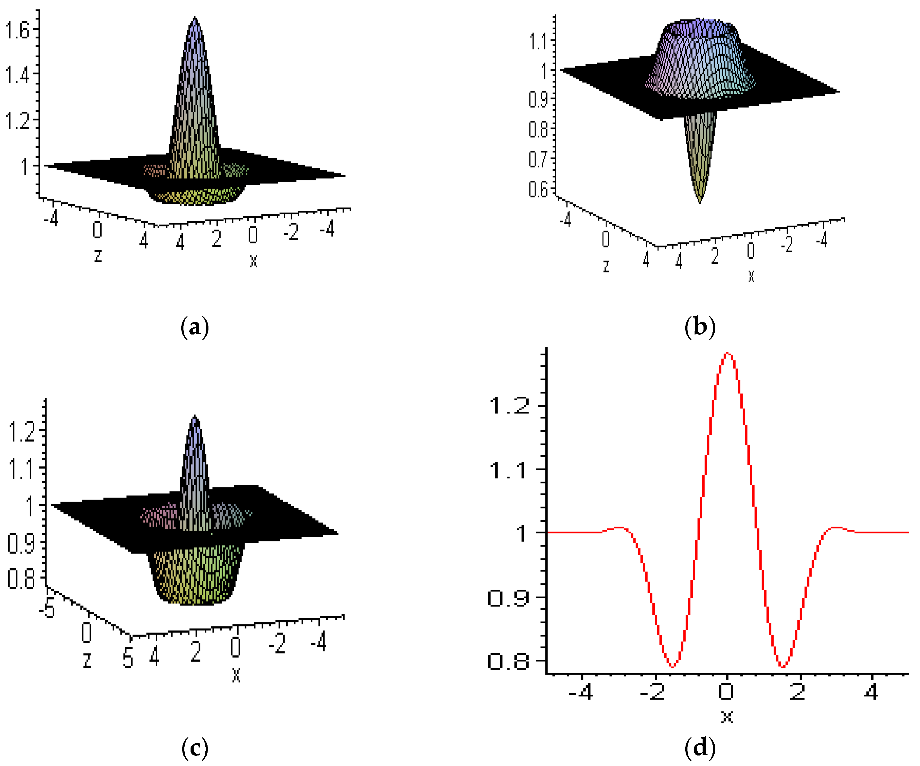
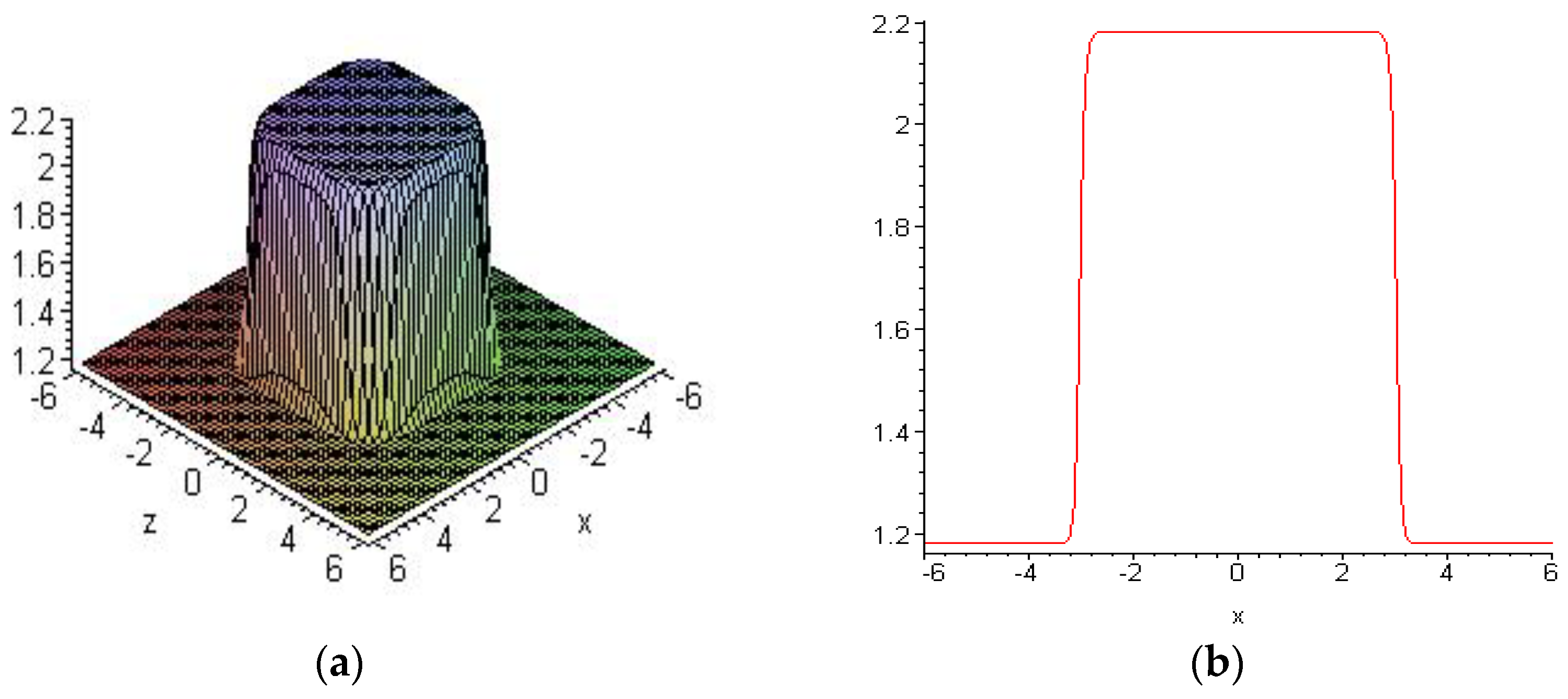
The arbitrary function $f(x,z,t)$ contained in the former resolutions indicates that the natural quantities $u,v,$ and $w$ have loaded constructions. For instance, rich localized excitements, e.g., lumps, instantons, dromions, ghostons, peakons, breathers, compactons, fractal and chaotic patterns, ring solitons, and their interactions [6,7,8,9], may be obtained by the potential U ≡ u_{15, x}, which is ignored in this paper because comparable situations were reported in the literature [6,7,8,9]. The present paper discusses some novel localized excitations, including the taper-like solitons, rectangle-soliton, plateau-type ring solitons, embed-solitons, as well as their interactions which has many applications in applied physics with the light of $U\equiv u_{15,x},$ namely

$$U\equiv u_{15}=\frac{k{B}^2}{f+ky},$$

(31)

in which $f\equiv f(x,z,t)$ represents an optional function of the highlighted variables, using the golden mean (golden ratio), symmetrical hyperbolic, and triangular Fibonacci functions.

6.1. Embed-Solitons

The authors of [10] discussed some embed-solitons. These excitations can be found in the (3+1)-dimensional Burgers structure. We choose f (x, z, t) as

$$f=\frac{1}{1+{\alpha }^{-x^2-z^2}\mathrm{sTFs}(x^2+z^2-t^2)},$$

(32)

After that, we get the embed-soliton for the natural field $U$ represented by the quantities Equation (31) having the fixed parameter $B=k=1,y=0$. Figure 1 illustrates the evolutional time profiles of the embed-soliton.

Identically, if we choose $f(x,z,t)$ to be

$$f=\frac{1}{1-{\left(\sec \mathrm{Fs}(x^2+z^2-t^2)\right)}_t},$$

(33)

and

$$f=\frac{1}{{\left({\alpha }^{-x^2-z^2}\mathrm{sTFs}(x^2+z^2-t^2)\right)}_{xxzz}},$$

(34)

we obtain two forms of embed-solitons for the natural field U in Equation (31) (see Figure 2 and Figure 3, respectively).

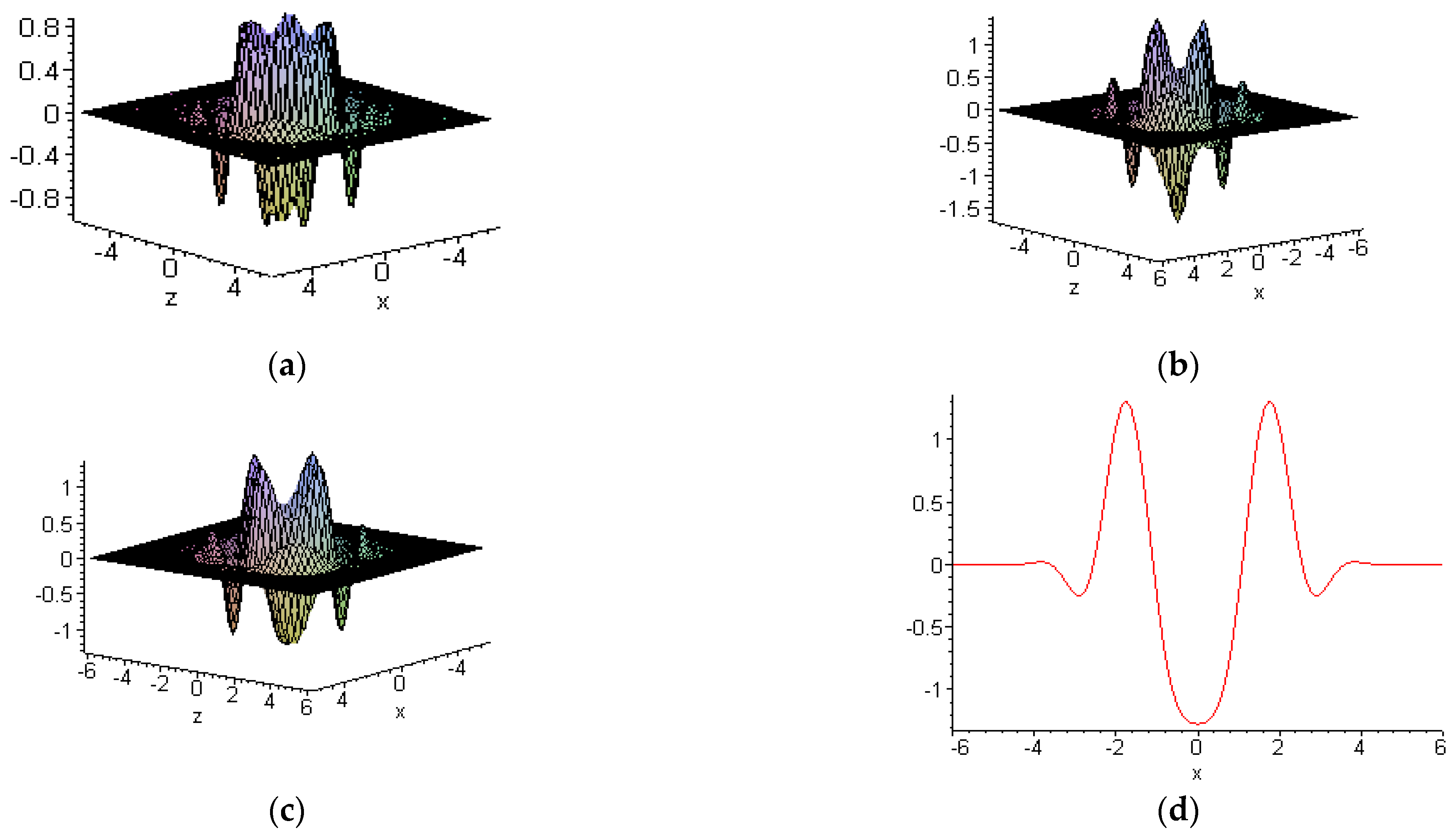
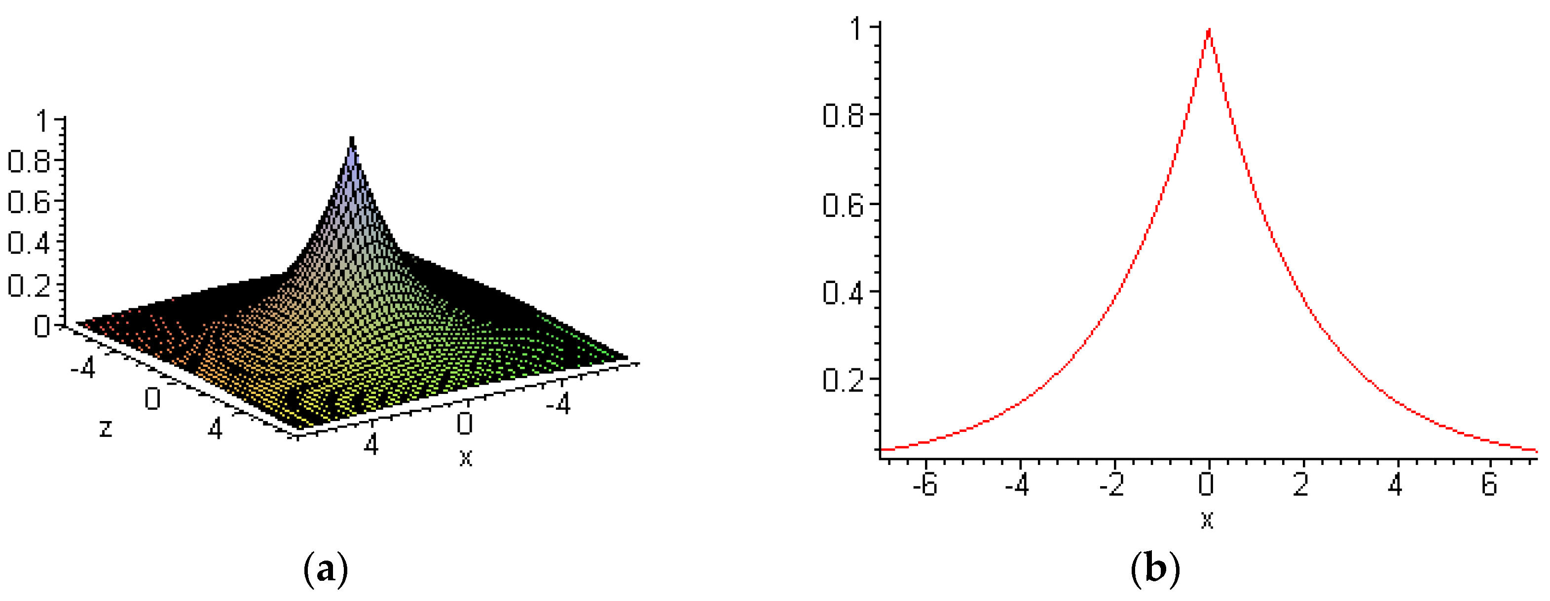
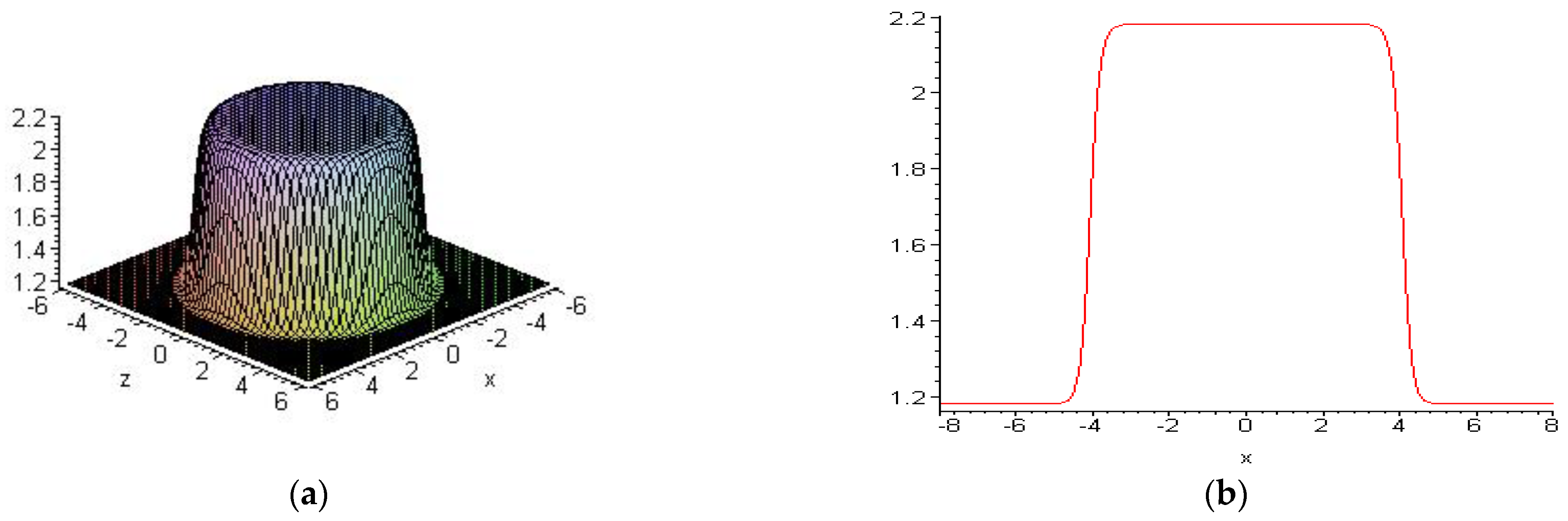
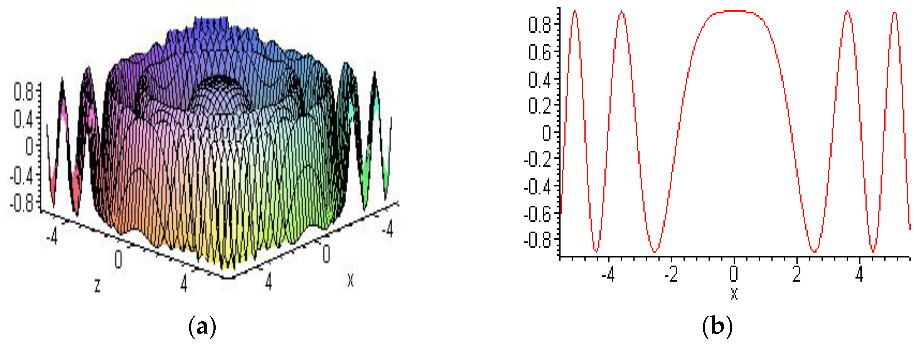
6.2. Other New Solitons

When considering $f(x,z,t)$ to be

$$\mathit{f}={\mathit{\alpha }}^{\sqrt{{\mathit{x}}^{\mathbf{2}}\mathbf{+}{\mathit{z}}^{\mathbf{2}}}}$$

(35)

we get a taper-like soliton for the natural field $U$ of Equation (31); see Figure 4.

Also, if we choose $f(x,z,t)$ to be

$$f=\frac{1}{2.8-{\alpha }^{\mathrm{tFs}(x^2+z^2-16)}}$$

(36)

we get a plateau-type ring soliton from natural field $U$ in Equation (31); see Figure 5.

Furthermore, by considering $f(x,z,t)$ to be

$$f=\frac{1}{2.8-{\alpha }^{\mathrm{tFs}(0.2x^4+0.2z^4-16)}}$$

(37)

we have a rectangle-soliton from the natural field $U$ of Equation (31) introduced in Figure 6.

By taking $f(x,z,t)$ to be

$$f=\frac{1}{\mathrm{cTFs}(x^2+z^2)}$$

(38)

we get periodic wave excitements for the natural field U in Equation (31) introduced in Figure 7.

Also, by considering $f(x,z,t)$ to be

$$f=\frac{1}{\mathrm{sTFs}(x^2+z^2)}$$

(39)

we have another periodic wave excitement for the natural field U in Equation (31) introduced in Figure 8.

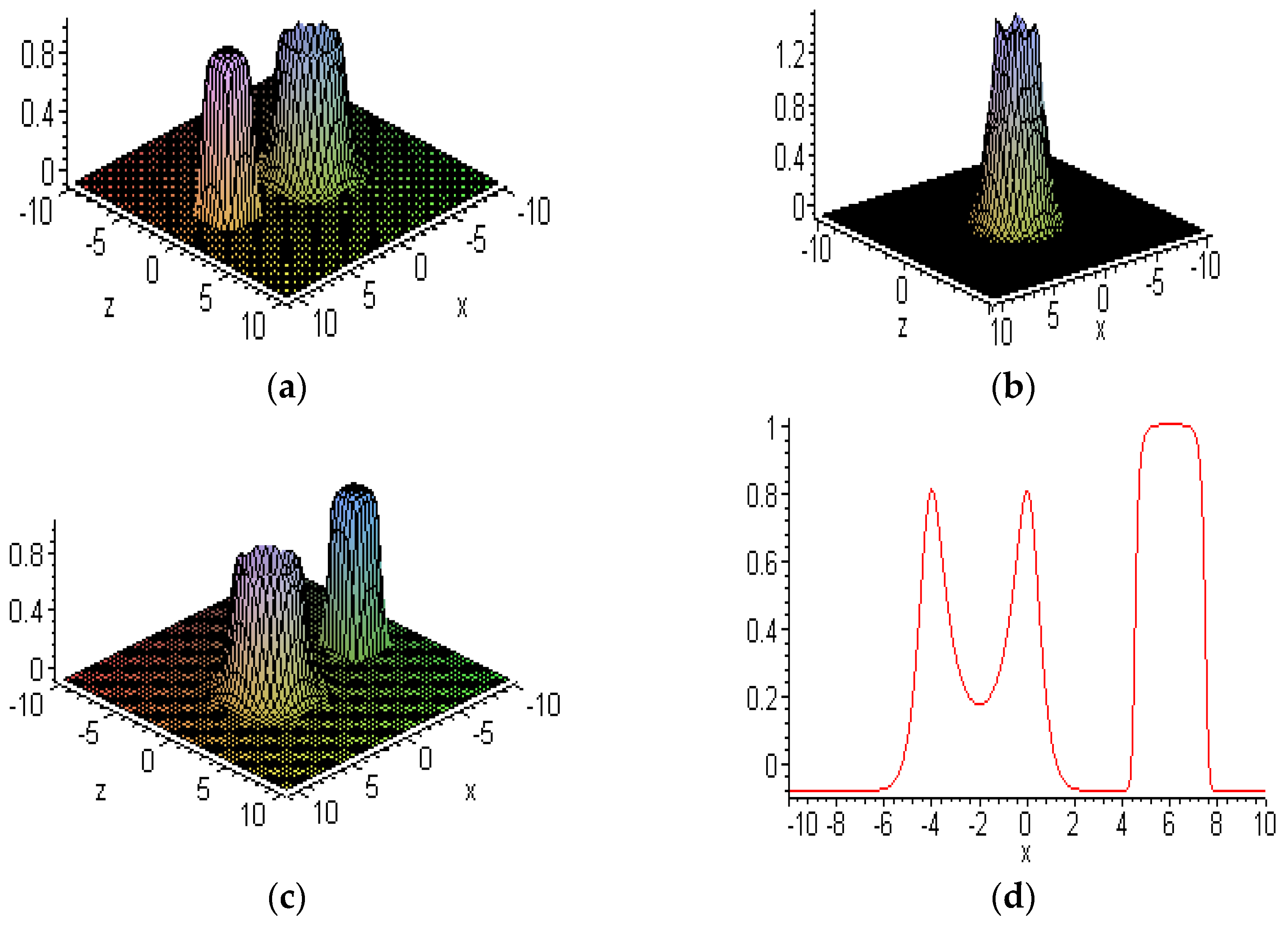
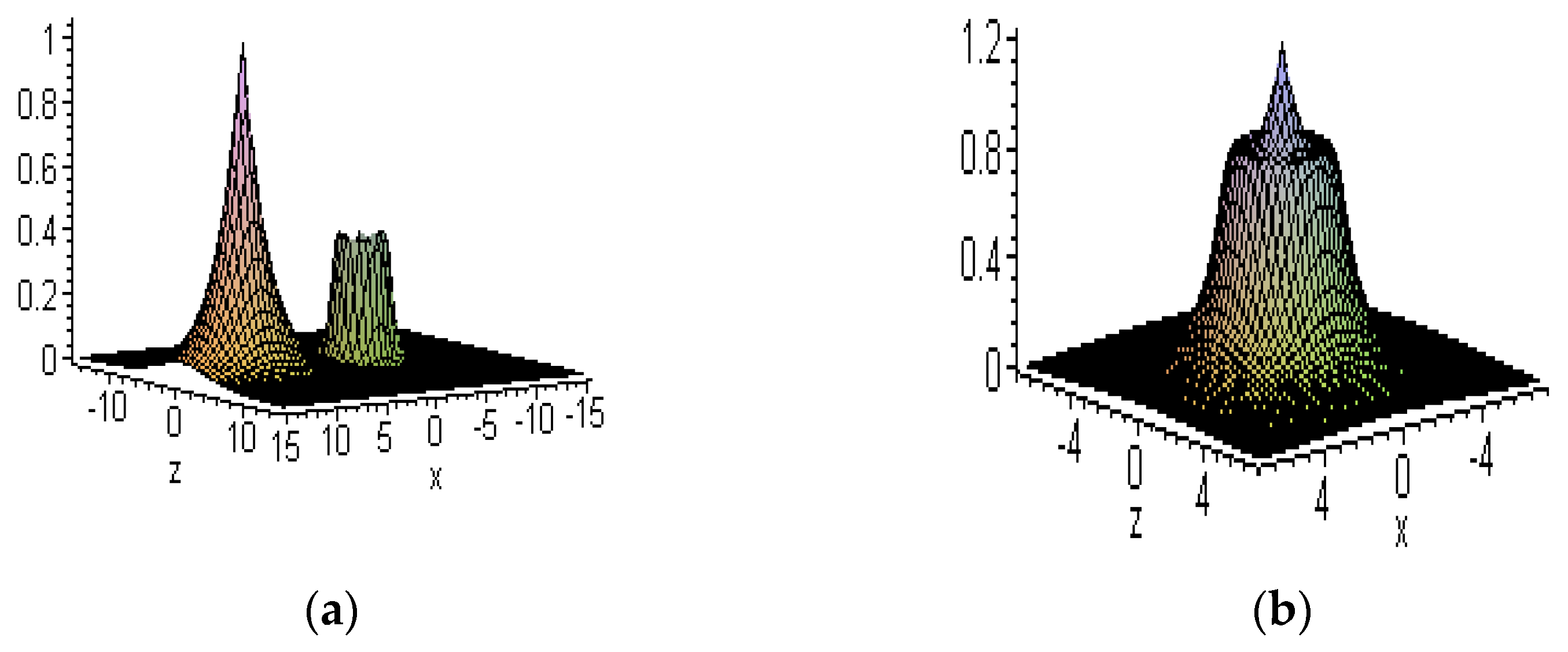
6.3. Interactions between Embedded and other Solitons

We considered the evolutional performance of the new embedded solitons. First, by taking into account the interaction between a rectangle and an embedded soliton. If $f(x,z,t)$ takes the form of

$$f=\frac{1}{1.7+\sec \mathrm{Fs}((x-t{)}^2+z^2-4)-1.1{\alpha }^{[\mathrm{tFS}((x+3t{)}^4+z^4-4)]}}$$

(40)

we get a rectangle and an embedded soliton concerning the natural field U in Equation (31), see Figure 9, and the detailed analysis illustrated that the interaction between the rectangle and embedded solitons is totally elastic as the wave shapes, velocities, and amplitudes are unchanged after the collision.

Therefore, we take into account the second case, the interaction of the embedded soliton and the plateau-type ring soliton. If $f(x,z,t)$ takes

$$f=\frac{1}{1.9+\sec \mathrm{Fs}((x-t{)}^2+z^2-4)-1.1{\alpha }^{[\mathrm{tFS}((x+3t{)}^2+z^2-4)]}}$$

(41)

Embedded and plateau-type ring solitons are obtained based on the natural field U in Equation (31). Figure 10 illustrates that the interaction among the embedded and plateau-type ring solitons is entirely elastic because their wave shapes, velocities, and amplitudes are unchanged after the collision.

We also take into account the third case of the interaction among taper-like and embedded soliton. When $f(x,z,t)$ takes the form of

$$f=\frac{1}{0.45\sec \mathrm{Fs}({(x-t)}^2+z^2-4)-1.1{\alpha }^{\sqrt{{(x+3t)}^2+z^2}}},$$

(42)

We obtain embedded and taper-like solitons of the natural field U in Equation (31), introduced by Figure 11. The embedded-taper-like soliton interaction becomes elastic because their wave shapes, velocities, and amplitudes remain stable after the collision.

7. Summary and Discussion

We developed and used the FR approach to arrive at innovative solutions to the Burgers model in (3+1)-dimensional. These answers aided in the explanation of several practical physical concerns. Unlike the FR approach, ours offered additional advantages. To begin, all NLPDEs are readily solved using the tanh-function and extended tanh-function approaches [17]. More crucially, we deduced innovative and more generic solutions to certain equations. Second, in a Riccati equation, A and B were selected to show the kinds and number of traveling wave solutions for NLPDEs. Thirdly, the system was computerized, enabling the computer to do lengthy and complicated algebraic computations. The Burgers structure in (3+1)-dimensional was effectively resolved using the FR and the linear separation variable structure. We got novel types of localized coherent excitements in the presence of the separation variable solution with arbitrary functions, including taper-like solitons and embed-solitons for the Burgers system in (3+1)-dimensional.

Meanwhile, we explored the evolutionary aspects of the embedded-soliton interaction with other kinds. The study demonstrated the elastic nature of interactions between rectangle solitons, taper-like solitons, plateau-type ring solitons, as well as embed-solitons. We anticipated that the embed-solitons would aid future research into the world’s complexity. To the authors’ knowledge, the taper-like solitons, embed-solitons, as well as their evolutionary properties have not been discussed in the literature for (3+1)-dimensional Burgers systems utilizing the golden proportion (golden mean or golden ratio), symmetrical hyperbolic, and triangular Fibonacci functions. However, future studies would examine the many possible uses of soliton theory in order to enrich the knowledge of innovative solitons and their associated evolutionary traits, notably their applications. We think that embedded solitons are a public entity in nonlinear wave systems and have potential applications in the future. In future work, we will try to use the method of the simplest equation, introduced by Kudryashov [54], or the modification of this method, proposed by Vitanov, Dimitrova and Kantz [55], to study the localized excitation. When $\alpha =e$, the results obtained in Ref [48] are recovered. To readers interested in studying localized excitation and symmetrical Lucas function, we recommended Ref. [49] and references there in.

References

1. Chang, Z.; Kong, L.; Cao, Y.; Liu, A.; Li, Z.; Wu, Q.; Huang, J.; Gao, L.; Zhu, T. Real-time dynamics of optical controlling for bound states of mode-locked fiber laser with short-range interaction. Opt. Laser Technol. 2022, 149, 107859. [Google Scholar] [CrossRef]
2. Wang, X.; Xing, Y.; Chen, G.; Lin, X.; Zhang, Z.; Zhu, Q.; Peng, J.; Li, H.; Dai, N.; Li, J. Temporal optical rogue waves in high power short-cavity Yb-doped random fiber laser. Opt. Laser Technol. 2022, 149, 107797. [Google Scholar] [CrossRef]
3. Pakzad, H.R.; Nobahar, D. Dust-ion acoustic solitons in superthermal dusty plasmas. New Astron. 2022, 93, 101752. [Google Scholar] [CrossRef]
4. Shen, M.; Li, X.; Zhang, Y.; Yang, X.; Chen, S. Effects of the interfacial Dzyaloshinskii-Moriya interaction on magnetic dynamics. J. Phys. D Appl. Phys. 2022, 55, 213002. [Google Scholar] [CrossRef]
5. Younas, U.; Bilal, M.; Ren, J. Diversity of exact solutions and solitary waves with the influence of damping effect in ferrites materials. J. Magn. Magn. Mater. 2022, 549, 168995. [Google Scholar] [CrossRef]
6. Islam, M.N.; Ilhan, O.A.; Akbar, M.A.; Benli, F.B.; Soybaş, D. Wave propagation behavior in nonlinear media and resonant nonlinear interactions. Commun. Nonlinear Sci. Numer. Simul. 2022, 108, 106242. [Google Scholar] [CrossRef]
7. Kengne, E.; Liu, W. Modulational instability and sister chirped femtosecond modulated waves in a nonlinear Schrodinger equation with self-steepening and self-frequency shift. Commun. Nonlinear Sci. Numer. Simul. 2022, 108, 106240. [Google Scholar] [CrossRef]
8. Dong, J.; Ling, L.; Zhang, X. Kadomtsev-Petviashvili equation: One-constraint method and lump pattern. Phys. D Nonlinear Phenom. 2022, 432, 133152. [Google Scholar] [CrossRef]
9. Weng, W.; Zhang, G.; Zhang, M.; Zhou, Z.; Yan, Z. Semi-rational vector rogon-soliton solutions and asymptotic analysis for any n-component nonlinear Schrodinger equation with mixed boundary conditions. Phys. D Nonlinear Phenom. 2022, 432, 133150. [Google Scholar] [CrossRef]
10. Sheng, H.H.; Yu, G.F. Solitons, breathers and rational solutions for a (2+1)-dimensional dispersive longwave system. Phys. D Nonlinear Phenom. 2022, 432, 133140. [Google Scholar] [CrossRef]
11. Didenkulova, E. Mixed turbulence of breathers and narrowband irregular waves: mKdV framework. Phys. D Nonlinear Phenom. 2022, 432, 133130. [Google Scholar] [CrossRef]
12. Wang, X.; Wang, L.; Liu, C.; Guo, B.; Wei, J. Rogue waves, semirational rogue waves and W-shaped solitons in the three-level coupled Maxwell-Bloch equations. Commun. Nonlinear Sci. Numer. Simul. 2022, 107, 106172. [Google Scholar] [CrossRef]
13. Sun, Y.L.; Chen, J.; Ma, W.X.; Yu, J.P.; Khalique, C.M. Further study of the localized solutions of the (2+1)-dimensional B-Kadomtsev-Petviashvili equation. Commun. Nonlinear Sci. Numer. Simul. 2022, 107, 106131. [Google Scholar] [CrossRef]
14. Tian, H.Y.; Tian, B.; Sun, Y.; Zhang, C.R. Three-component coupled nonlinear Schrodinger system in a multimode optical fiber: Darboux transformation induced via a rank-two projection matrix. Commun. Nonlinear Sci. Numer. Simul. 2022, 107, 106097. [Google Scholar] [CrossRef]
15. Dikande, A.M. On a Model for Nerve Impulse Generation Mediated by Electromechanical Processes. Braz. J. Phys. 2022, 52, 41. [Google Scholar] [CrossRef]
16. Lavanya, C. Propagation and Soliton Collision of Positron Acoustic Waves in Four-component 208 Space Plasmas. Braz. J. Phys. 2022, 52, 38. [Google Scholar] [CrossRef]
17. Kumar, S.; Dhiman, S.K. Lie symmetry analysis, optimal system, exact solutions and dynamics of solitons of a (3+1)-dimensional generalised BKP–Boussinesq equation. Pramana 2022, 96, 31. [Google Scholar] [CrossRef]
18. Nisar, K.S.; Inc, M.; Jhangeer, A.; Muddassar, M.; Infal, B. New soliton solutions of Heisenberg ferromagnetic spin chain model. Pramana 2022, 96, 28. [Google Scholar] [CrossRef]
19. Houwe, A.; Rezazadeh, H.; Bekir, A.; Doka, S.Y. Traveling-wave solutions of the Klein–Gordon equations with M-fractional derivative. Pramana 2022, 96, 26. [Google Scholar] [CrossRef]
20. Alam, M.S.; Talukder, M.R. Characteristic behaviour of N-order ion acoustic rogue waves solution in electron-positron-ion plasmas. Plasma Res. Express 2022, 4, 015001. [Google Scholar] [CrossRef]
21. Cisneros-Ake, L.A. Stability of multi-hump localized solutions in the Holstein model for linear acoustic and soft nonlinear optical interactions. Phys. D Nonlinear Phenom. 2022, 431, 133138. [Google Scholar] [CrossRef]
22. Kudryashov, N.A. Bright and dark solitons in a nonlinear saturable medium. Phys. Lett. A 2022, 427, 127913. [Google Scholar] [CrossRef]
23. Chandramouli, S.; Farhat, A.; H Musslimani, Z. Time-dependent Duhamel renormalization method with multiple conservation and dissipation laws. Nonlinearity 2022, 35, 1286–1310. [Google Scholar] [CrossRef]
24. Sudhakar, S.; Vignesh Raja, S.; Govindarajan, A.; Batri, K.; Lakshmanan, M. Low-power optical bistability in PT-symmetric chirped Bragg gratings with four-wave mixing. J. Opt. Soc. Am. B Opt. Phys. 2022, 39, 643. [Google Scholar] [CrossRef]
25. Perna, S.; Bruckner, F.; Serpico, C.; Suess, D.; d’Aquino, M. Computational micromagnetics based on normal modes: Bridging the gap between macrospin and full spatial discretization. J. Magn. Magn. Mater. 2022, 546, 168683. [Google Scholar] [CrossRef]
26. Seadawy, A.R.; Rizvi, S.T.R.; Mustafa, B.; Ali, K.; Althubiti, S. Chirped periodic waves for an cubic-quintic nonlinear Schrodinger equation with self steepening and higher order nonlinearities. Chaos Solitons Fractals 2022, 156, 111804. [Google Scholar] [CrossRef]
27. Velasco-Juan, M.; Fujioka, J. Lagrangian nonlocal nonlinear Schrodinger equations. Chaos Solitons Fractals 2022, 156, 111798. [Google Scholar] [CrossRef]
28. Sugati, T.G.; Seadawy, A.R.; Alharbey, R.A.; Albarakati, W. Nonlinear physical complex hirota dynamical system: Construction of chirp free optical dromions and numerical wave solutions. Chaos Solitons Fractals 2022, 156, 111788. [Google Scholar] [CrossRef]
29. Li, Q.; Shan, W.; Wang, P.; Cui, H. Breather, lump and N-soliton wave solutions of the (2+1)-dimensional coupled nonlinear partial differential equation with variable coefficients. Commun. Nonlinear Sci. Numer. Simul. 2022, 106, 106098. [Google Scholar] [CrossRef]
30. Evslin, J.; Halcrow, C.; Romanczukiewicz, T.; Wereszczynski, A. Spectral Walls at One Loop. arXiv 2022, arXiv:2202.08249. [Google Scholar] [CrossRef]
31. Sreedharan, A.; Kuriyattil, S.; Wuster, S. Hyper-entangling mesoscopic bound states. arXiv 2022, arXiv:2202.06120. [Google Scholar]
32. Evslin, J. Moving Kinks and Their Wave Packets. arXiv 2022, arXiv:2202.04905. [Google Scholar] [CrossRef]
33. He, Y.; Slunyaev, A.; Mori, N.; Chabchoub, A. Experimental evidence of nonlinear focusing in standing water waves. arXiv 2022, arXiv:2202.04775. [Google Scholar] [CrossRef] [PubMed]
34. Muller-Hoissen, F. Binary Darboux transformation of the first member of the nega- tive part of the AKNS hierarchy and solitons. arXiv 2022, arXiv:2202.04512. [Google Scholar]
35. Zabolotnykh, A.A. Plasma solitons in gated two-dimensional electron systems: Exactly solvable analytical model for the regime beyond weak non-linearity. arXiv 2022, arXiv:2202.04503. [Google Scholar] [CrossRef]
36. Lei, Z.; Ren, X.; Yang, Z. Radiation of the energy-critical wave equation with compact support. arXiv 2022, arXiv:2202.02045. [Google Scholar]
37. Jin, H.-Y.; Wang, Z.-A.; Wu, L. Global dynamics of a three-species spatial food chain model. J. Differ. Equ. 2022, 333, 144–183. [Google Scholar] [CrossRef]
38. Wang, Y.; Wu, H.; Ruan, S. Global dynamics and bifurcations in a four-dimensional replicator system. Discret. Contin. Dyn. Syst.-B 2013, 18, 259–271. [Google Scholar] [CrossRef]
39. Jin, H.-Y.; Wang, Z.-A. Global stabilization of the full attraction-repulsion Keller-Segel system. Discret. Contin. Dyn. Syst. 2020, 40, 3509–3527. [Google Scholar] [CrossRef] [Green Version]
40. Li, Q.-K.; Lin, H.; Tan, X.; Du, S. H Consensus for Multiagent-Based Supply Chain Systems under Switching Topology and Uncertain Demands. IEEE Trans. Syst. Man Cybern. Syst. 2020, 50, 4905–4918. [Google Scholar] [CrossRef]
41. Li, X.; Sun, Y. Stock intelligent investment strategy based on support vector machine parameter optimization algorithm. Neural Comput. Appl. 2020, 32, 1765–1775. [Google Scholar] [CrossRef]
42. Shao, Z.; Zhai, Q.; Han, Z.; Guan, X. A linear AC unit commitment formulation: An application of data-driven linear power flow model. Int. J. Electr. Power Energy Syst. 2023, 145, 108673. [Google Scholar] [CrossRef]
43. Cai, Y.-J.; Wu, J.-W.; Lin, J. Nondegenerate N-soliton solutions for Manakov system. Chaos Solitons Fractals 2022, 164, 112657. [Google Scholar] [CrossRef]
44. Liu, Y.; Ren, B.; Wang, D.-S. Localised Nonlinear Wave Interaction in the Generalised Kadomtsev-Petviashvili Equation. East Asian J. Appl. Math. 2021, 11, 301–325. [Google Scholar] [CrossRef]
45. Liu, Y.; Peng, L. Some novel physical structures of a (2+1)-dimensional variable-coefficient Korteweg–de Vries system. Chaos Solitons Fractals 2023, 171, 113430. [Google Scholar] [CrossRef]
46. Saleh, M.H.; Altwaty, A.A. Optical solitons of the extended Gerdjikov-Ivanov Equation in DWDM system by extended simplest equation method. Appl. Math. Inf. Sci. 2020, 14, 901–907. [Google Scholar] [CrossRef]
47. Mirzazadeh, M.; Eslami, M.; Bhrawy, A.H.; Ahmed, B. Biswas, Anjan, Solitons and other solutions to Complex-Valued Klein-Gordon equation in ϕ-4 field theory. Appl. Math. Inf. Sci. 2015, 9, 2793–2801. [Google Scholar]
48. Zhu, H.-P.; Zheng, C.-L. Embed-Solitons and their evolutional behaviors of (3+1)-dimensional Burgers System. Commun. Theor. Phys. 2007, 48, 57–62. [Google Scholar] [CrossRef]
49. Abdel-Salam, E.A.-B. Quasi-periodic structures based on symmetrical lucas Function of (2+1)-dimensional modified dispersive water-wave system. Commun. Theor. Phys. 2009, 52, 1004. [Google Scholar] [CrossRef]
50. Friedman, I.; Riano, O.; Roudenko, S.; Son, D.; Yang, K. Well-posedness and dynamics of solutions to the generalized KdV with low power nonlinearity. arXiv 2022, arXiv:2202.01130. [Google Scholar] [CrossRef]
51. Ali, U.; Ahmad, H.; Baili, J.; Botmart, T.; Aldahlan, M.A. Exact analytical wave solutions for space-time variable-order fractional modified equal width equation. Results Phys. 2022, 33, 105216. [Google Scholar] [CrossRef]
52. Bilal, M.; Ahmad, J. A variety of exact optical soliton solutions to the generalized (2+1)-dimensional dynamical conformable fractional Schrodinger model. Results Phys. 2022, 33, 105198. [Google Scholar] [CrossRef]
53. Nisar, K.S.; Ali, K.K.; Inc, M.; Mehanna, M.S.; Rezazadeh, H.; Akinyemi, L. New solutions for the generalized resonant nonlinear Schrodinger equation. Results Phys. 2022, 33, 105153. [Google Scholar] [CrossRef]
54. Kudryashov, N.A. Simplest equation method to look for exact solutions of nonlinear differential equations. Chaos Solitons Fractals 2005, 24, 1217–1231. [Google Scholar] [CrossRef] [Green Version]
55. Vitanov, N.K.; Dimitrova, Z.I.; Kantz, H. Modified method of simplest equation and its application to nonlinear PDEs. Appl. Math. Comput. 2010, 216, 2587–2595. [Google Scholar] [CrossRef]
Figure 1. Evolutional graphs of the embed-soliton for the field U , as shown in Equation (31) conditional upon Equation (32) and B = k = 1 , y = 0 at times: (a) t = 20 , (b) t = 1 , (c) t = 4.5 , (d) A sectional view associated with (c) at z = 0 .
Symmetry 15 01473 g001
Figure 2. Evolutional graphs of the embed-soliton for the field, as shown in Equation (31) conditional upon Equation (33) and B = k = 1 , y = 0 at times: (a) t = 2 , (b) t = 0.1 , (c) t = 2 , (d) A sectional view associated with (c) at z = 0 .
Symmetry 15 01473 g002
Figure 3. Evolutional graphs of the embed-soliton for the field U , as shown in Equation (31) conditional upon Equation (34) and B = k = 1 , y = 0 at times: (a) t = 2 , (b) t = 0 , (c) t = 1.2 , (d) A sectional view associated with (c) at z = 0 .
Symmetry 15 01473 g003
Figure 4. (a) A plot of taper-like soliton for the field U , as shown in Equation (31) conditional upon Equation (35) and B = k = 1 , y = 0 (b) A sectional view associated with (b) at z = 0 .
Symmetry 15 01473 g004
Figure 5. (a) A plot of plateau-type ring soliton for the field U , as shown in Equation (31) conditional upon Equation (36) and B = k = 1 , y = 0 (b) A sectional view associated with (a) at z = 0 .
Symmetry 15 01473 g005
Figure 6. (a) A plot of rectangle-soliton for the field U , as presented in Equation (31) conditional upon Equation (37) and B = k = 1 , y = 0 (b) A sectional view associated with (a) at z = 0 .
Symmetry 15 01473 g006
Figure 7. (a) A plot of the periodic wave excitements for the field U , as shown in Equation (31) conditional upon Equation (38) and B = k = 1 , y = 0 (b) A sectional view associated with (a) at z = 0 .
Symmetry 15 01473 g007
Figure 8. (a) A plot of the periodic wave excitements for the field U in Equation (31) conditional upon Equation (39) and B = k = 1 , y = 0 (b) A sectional view associated with (a) at z = 0 .
Symmetry 15 01473 g008
Figure 9. The time evolutional graphs of the interaction among embed and rectangle soliton for the field U in Equation (31) conditional upon Equation (40) and B = k = 1 , y = 0 at times: (a) t = 2 , (b) t = 0 , (c) t = 2 , (d) A sectional view associated with (a) at z = 0 .
Symmetry 15 01473 g009
Figure 10. Time evolutional profiles of the interaction among embedded and plateau-type ring soliton for the field U in Equation (31) conditional upon Equation (41) and B = k = 1 , y = 0 at times: (a) t = 2 , (b) t = 0 , (c) t = 2 , (d) A sectional view associated with (a) at z = 0 .
Symmetry 15 01473 g010
Figure 11. Time evolutional profiles of the interaction among embedded and taper-like ring soliton for the field U in Equation (31) conditional upon Equation (42) and B = k = 1 , y = 0 at times: (a) t = 3 , (b) t = 0 , (c) t = 3 , (d) A sectional view associated with (a) at z = 0 .
Symmetry 15 01473 g011aSymmetry 15 01473 g011b
Disclaimer/Publisher’s Note: The statements, opinions and data contained in all publications are solely those of the individual author(s) and contributor(s) and not of MDPI and/or the editor(s). MDPI and/or the editor(s) disclaim responsibility for any injury to people or property resulting from any ideas, methods, instructions or products referred to in the content.