Abstract
The model predictive control (MPC) technique is widely employed in process industries as a control scheme. The quality of the model used greatly influences the performance of the MPC. In time-varying systems, the plant model plays a critical role in determining the controller’s performance, as the controller’s control action relies on an adaptive model. Therefore, updating the system parameters rapidly and symmetrically in time-varying systems becomes necessary. To address this need, in the proposed work, a non-minimal state space model of a time-varying system is utilized for parameter estimation, and these parameters are updated at every sampling instant using a multi-innovation recursive least squares (MIRLS) scheme, which enables the timely updates of system parameters. We have explored various extensions of the recursive least square (RLS) scheme, such as the multi-innovation recursive least squares (MIRLS) method. This extension aims to achieve a higher convergence rate for parameter estimation. Furthermore, we have focused on the parameter estimation of a non-minimal state space time-varying system, where the system parameters change at each time interval. Additionally, we have incorporated a time-varying objective function into the MPC formulations, which enables adaptability to change the system dynamics. To demonstrate the applicability of our proposed approach, we have conducted simulation experiments using a benchmark time-varying model. These experiments showcase the effectiveness and benefits of our proposed methodology in dealing with time-varying systems.
1. Introduction
Adaptive model predictive control (AMPC) is an advance control strategy of MPC that incorporates adaptive techniques to enhance the system model’s performance by symmetrically adapting the changing system’s parameters. MPC is a widely applied control technique commonly used in the process industry [1,2]. MPC defines an approach for control engineers to define their strategy according to their needs. The standard transfer function representation cannot fully reveal the true behavior of the states inside the system, such as controllability and observability. Therefore, the transfer function model is not always suitable for stability analysis of time-varying systems. The state space model, which utilizes state feedback for control purposes, overcomes these limitations. MPC can handle constraints, including input and output constraints [3]. The proposed MPC design can effectively handle constraints for large-scale time-varying systems. In this work, the constraints are explicitly addressed by solving a quadratic problem in real-time to predict future outcomes. The quality of the prediction model depends on the accuracy of the model itself. A poorly defined model cannot generate a good estimate for the controller, and consequently, the control system’s performance is affected [4,5]. Typically, the finite impulse response (FIR) and impulse response models (IR) are used in time-varying systems, where the controller performance relies on the quality of the model. In time-varying systems, updated parameters are required at every sampling instant [6].
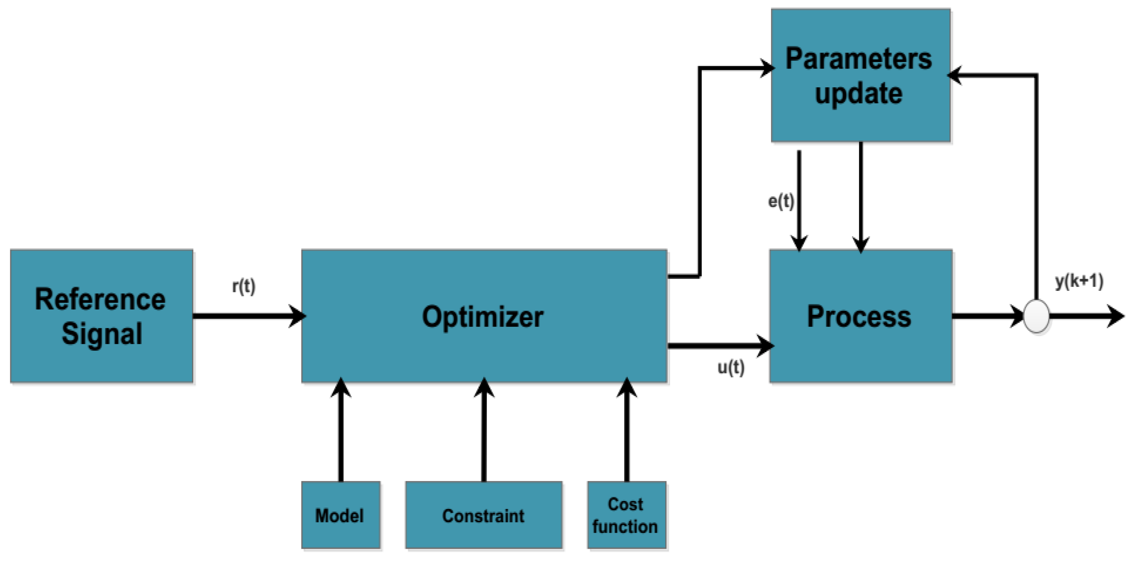
For an MPC controller, model identification is necessary, which can be achieved using commonly used techniques like system identification. System identification refers to the task of estimating parameters based on observations of the dynamic system. It involves designing, executing, and interpreting the results of experiments [7]. Generally, two types of techniques are adopted for constructing a model. The first method involves designing a mathematical model of the system by applying fundamental laws of physics, such as Newton’s law or Ohm’s law. The second method involves performing a series of experiments on the system to collect data for system identification [8]. After applying the system identification technique, a suitable model is designed for the system depending upon its behavior, like autoregressive (AR), autoregressive moving average (ARMA), autoregressive moving average exogenous (ARMAX), etc. In the proposed work, a non-minimal state space model (NMSS) of a time-varying system is used for the parameter estimation, and these parameters are updated at every sampling instant by using a MIRLS scheme. The commonly applied MPC control technique is based on the state space model, which uses a state-feedback controller and an observer. By applying the non-minimal state-space technique, it is possible to avoid the use of a state observer, which enhances the performance of the MPC in terms of efficiency and fast-tracking of future control trajectories. A commonly applied control scheme is shown in Figure 1, where r(t) is the reference signal, u(t) is the current input, e(t) is the error, and y(k+1) is the output of next time interval.

Figure 1.
Model predictive control.
Due to advancements in technology, the demands for performance and efficiency of control systems are growing rapidly. Fast convergence rate and parameter estimation are major challenges in such systems. In a system where online parameter estimation of a time-varying system is considered, the algorithm’s convergence rate becomes extremely important to achieve fast tracking. Several algorithms are available for parameter estimation, including RLS and stochastic gradient (SG) method, each with its advantages and drawbacks, such as slow or fast convergence rates or computational burden. In the proposed work, we present two different types of algorithms for parameter estimation of time-varying systems, providing a comparative analysis of computational burden and convergence rate.
2. Background and Literature Review
This section describes the background and literature review of different modeling schemes and parameter estimation techniques; hence, this section will cover many aspects of modeling, system identification, and parameter estimation techniques, which have been applied in various MPC domains. A system can be represented in many forms depending upon its behavior, like linear, nonlinear time-varying, time-invariant, etc. The model structure of a system can be represented with a lot of modeling schemes like output error model, AR, ARMAX, ARMA, ARIMAX, etc. In the proposed work, we used an ARMAX time series model for predicting the future forecast. Considering the plant consists of inputs and outputs, then the mathematical structure of the model can be captured by the differential equation in the form of an ARMAX model. Consider the model contains a time-varying error, which is a white noise of zero mean, a discrete-time model with inputs and outputs can capture the design used in the model by a difference, as shown in Equation (1).
represents the output at the next time step, ) is the output at time t, is the input at time t, and represents the time-varying error term at time t. The terms , ,…, are the coefficients associated with the past outputs ), and , ,…, are the coefficients associated with the past inputs . The parameters n and m determine the number of past samples considered in the model.
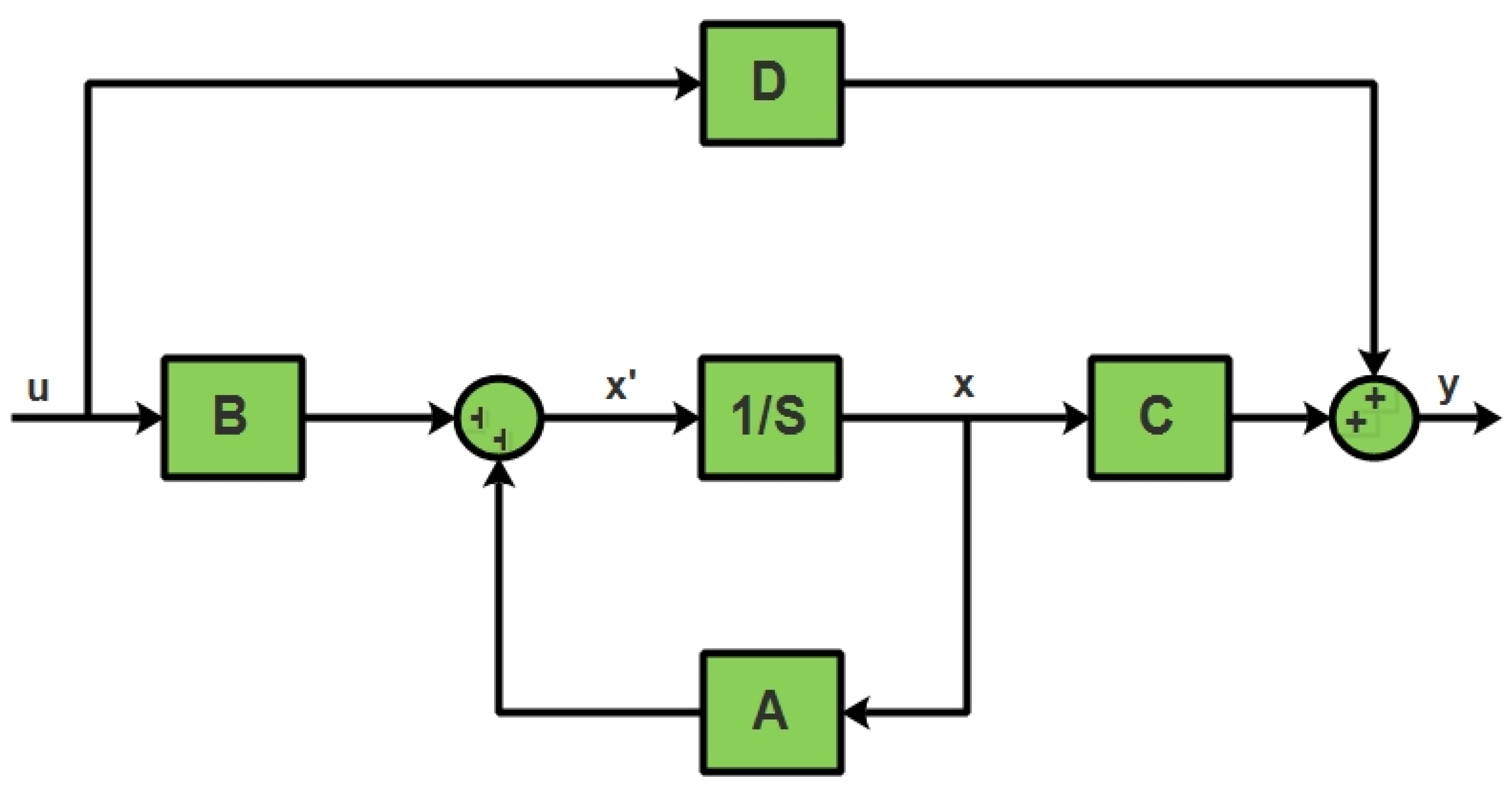
This difference equation captures the relationship between the inputs, outputs, and the time-varying error term in the ARMAX model, enabling the prediction of future forecasts based on past input–output data. A linear system that has a set of inputs, state variables, and output variables can be represented in the most common state space equation, as shown in Equation (2).
where the system matrix is denoted with A, the input matrix is denoted with B, and is the derivative of the state vector at instant k. The output vector is denoted by y(z), C is the output matrix, u(z) is the control or input matrix, and D is the feedforward matrix [9]. The state space model of the system is shown in Figure 2.
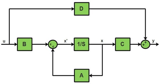
Figure 2.
State space model.
2.1. Non-Minimal State Space-Based MPC
The conventional method of MPC control based on the state space model uses a state-feedback controller and an observer. By applying the non-minimal state space technique, it is possible to avoid the use of a state observer, which improves the efficiency of the MPC scheme in terms of accuracy and convergence rate [10]. The system’s identification, in strict terms, refers to the task of estimating the parameters based on the observations and dynamics of the system. Identifying the system in broad terms refers to the many subtleties that arise when we design, execute, and interpret the results of this experiment [11]. In general, two types of techniques are adopted for constructing a model; that is, by applying the law of physics like Newton’s law or Ohm’s law, a mathematical model is designed, and the other one, called system identification, is by collecting data after performing several experiments on the system, with which we want to model this technique [12]. In the system identification technique, several inputs, u(t), are applied one by one to the system, and observe and record the output, y(t), of the corresponding inputs, u(t). The output, y(t), is a mixed signal of the output response of the system, which has some noise or disturbance, generally denoted by v(t). The block diagram of the general system identification technique is given in Figure 3a. Where input u(t) is a uniformly distributed signal, the simple parametric identification model of a system is a linear regression, which can be described below in Equation (3).
where is the estimated value of output at time t, y(t) is a measurable value, is a vector of unknown parameters, is the vector of a known quantity, and e(t) is the model error. t denotes the sampling instant. Several experiments are performed to collect the data, which are given to the system identification technique for modeling. Figure 3b shows the inputs applied to a system for identification, and Figure 3c shows the corresponding outputs of the system.

Figure 3.
System’s inputs and output response.
2.2. Model Representation
In the proposed work, an input u(t) and output y(t) are applied to a time-varying system, and these signals input u(t) and output y(t) are the discrete-time samples at k = 1, 2, 3, 4,…, N and the sampled values can be presented through a difference equation as follows:
where v(t) is the disturbance or noise if is the backward delay operator, i.e., , then the above Equation (2) can be represented as follows:
where
The system can be represented as a linear regression as follows:
If v(t) is a white noise and no input is present, then the above system becomes the following:
which is known as the AR process. The AR model is used in a stochastic process, which is used in statistics for estimations that depend on the weighted sum of the past value. There are two types of AR models. The first one is AR1 of a first-order process, meaning the existing values of the model depend on the recent preceding values. The second type AR2 depends on the past values and is called a second-order autoregressive process [13]. Another type is the ARMAX model, which is a traditional model used widely in the predicting field. Consider an ARMAX model with inputs u(t) and outputs y(t) is described as follows:
Let
Therefore
Now
where
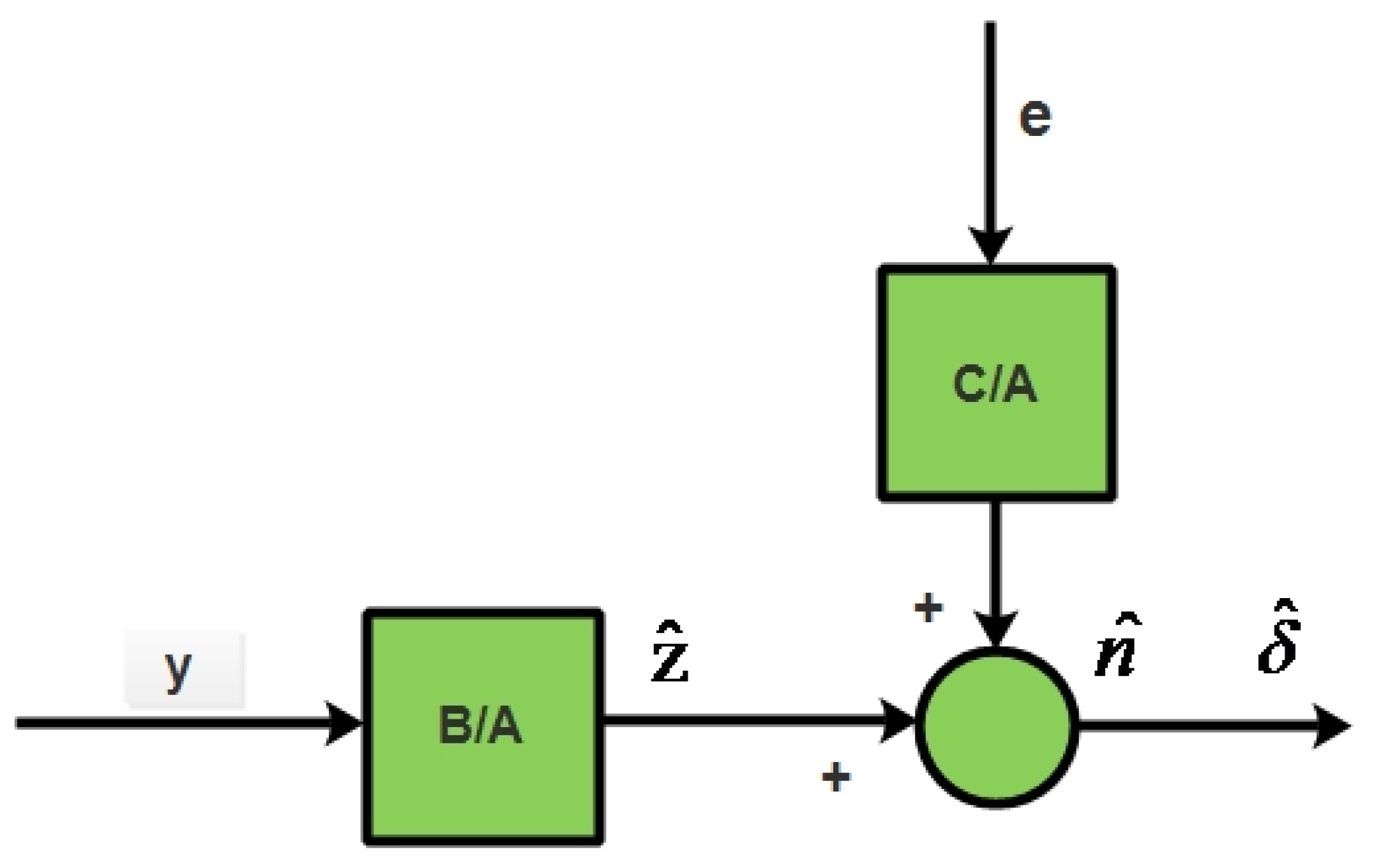
where e(t) is the white noise of sequence with variance . The ARMAX model structure can be represented in Figure 4.

Figure 4.
ARMAX mode.
2.3. Parameter Estimation
There are a lot of techniques for parameter estimation in control systems like RLS, MIRLS, Kalman filter stochastic gradient, etc. The recursive least square (RLS) is the most common technique to estimate the parameters, which recursively finds the coefficients of the parametric model. The RLS algorithm is well-known because of its high performance and fast convergence rate when dealing with a time-varying system. The RLS algorithm works excellently, but there are some issues like stability and computational burden [14]. Consider the system whose input and output data are recorded for a series of time means for a specific time span, as shown in Figure 3b,c; by analyzing these data, a mathematical model of the system can be written as under.
where is the output, is the input, and v is the disturbance at discrete-time .
This model can be written in more compact as given below:
where is the backwards shift, and A and B are the polynomials. This ARX model can be converted into regression form as follows:
where
which contains the previous outputs and inputs, and the unknown parameters can be written as follows:
In indirect adaptive control [15], we use the past information, Y(t), to estimate the parameters as shown in Equation (7).
To speed up the tracking of identification, a method called the forgetting factor can be used to converge the rate of the RLS algorithm and hence speed up the algorithm. Such a technique is commonly applied for online parameter estimation [16]. Multi-innovation recursive least square techniques are used to increase the efficiency and convergence rate of the algorithm. The MIRLS algorithm can be presented as follows:
where , , and are the innovation vectors, is the input vector, and is the covariance matrix [17]. The stochastic gradient (SG) is a popular technique due to its advantage in terms of computation burden, but the drawback of this technique is that its convergence rate is too slow, and the efficiency is also very low, especially when compared with the RLS algorithm. This algorithm can be represented in terms of a mathematical form as follows:
where , and are the innovation vectors, is the input vector, and is the covariance matrix [18].
2.4. MPC Modeling
Model selection is based on the observation and behavior of the system. MPC can define an approach for the control engineer to define their strategy according to their needs. The standard transfer function representation cannot reveal the true behavior of the states inside the system, like the controllability and observability, which is why the transfer function model cannot always be used for the stability analysis of the time-varying system. The state space model uses state feedback for control purposes. The MPC modeling scheme can also cope with constraints, such as input and output constraints [3]. Consider a single input and single output system as follows:
where u(k) is the input to the system and y(k) is the process output at sampling instant k.
Now, taking the difference operation on the above equation we receive the following:
and state variable difference is denoted by the following:
The control variable can also be represented in terms of a difference equation like the following:
after applying the difference on state variable and control variable we can modify the state space equation of the system as follows:
Now the augmented state space model, which used in the PC, is written as follows:
The triplet (A, B, C) is called the augmented model. The MPCs performance deteriorates due to constraints on the input, output, and control variables. To tackle these constraints, a quadratic optimization technique is applied in the MPC formulation to enhance its performance. If the control signal has some limitation in the system due to operational constraints in the plant, then this limitation prevents the control signal to be applied to the system when its amplitude crosses this limit. Consider the limitation on the control signal is as if ; and if where is a real number.
When this is applied to the system, and no attention is paid to the control saturation, the closed-loop response of the system may deteriorate in the presence of constraints. To handle these constraints, a small modification is required in the formulation. If the calculated value of the control signal, then and . If the calculated value of the control signal, then and . This updated is used in the observer to estimate the next state of the state variable.
This modification enhances the performance of the control system.
2.5. Non-Minimal State Space Representation
A lot of techniques are available for time-varying system modeling. In the proposed work, we used a non-minimal state space model for a time-varying system. Commonly, three types of approaches are used for MPC design, and every design approach uses a different model structure. The FIR and step-response model were popular in the past, the FIR-based model design consists of a DMC formulation, but there is a limitation in these models because they can only work for a stable system and they need a larger order [19]. In the proposed work, a non-minimal state space model of the time varying system is used to achieve the symmetric response. The advantage of the proposed non-minimal state space representation is that there is no need for an observer for the state estimation; hence it enhances the convergence rate of state estimation.
Let a system have the following form:
where the numerator and the denominator are presented in terms of backshift operator , i.e.,
Considering the model contains a time-varying error, which is a white noise of zero mean, a discrete-time model with G inputs and N outputs can capture the design used in the model by a difference equation.
Let be the variation in the error of the time-varying model.
; and . Where is the output difference and control variable. Respectively, these variation in the system can be found with the RLS algorithm [5,6]. In the similar way, the non-minimal state vector can be chosen, as shown in Equation (26).
and the above state space model can be defined as in Equation (27).
where
3. Methodology
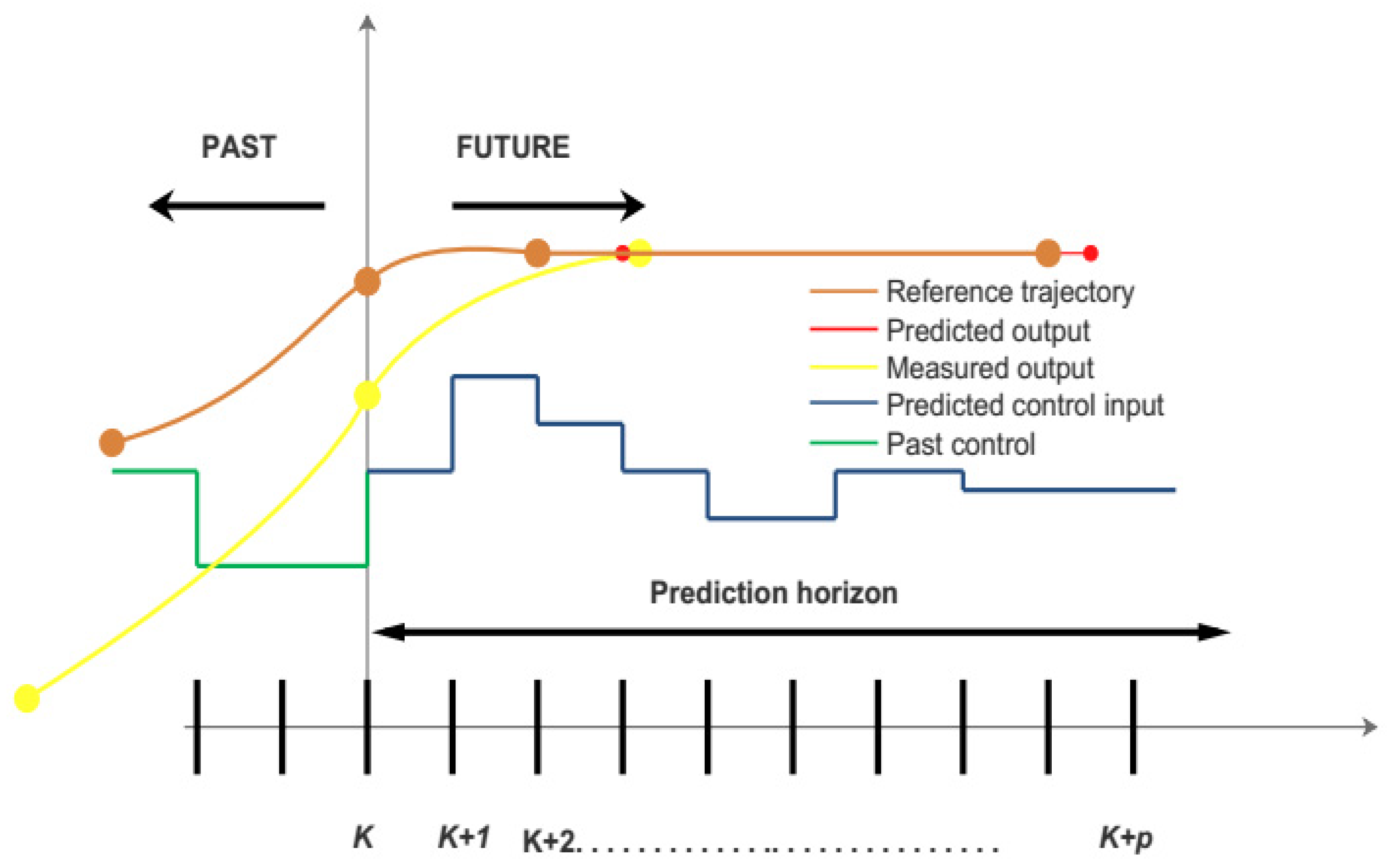
In this work, an adaptive MPC strategy is used for a system that varies over the time with input, output, and control variable constraints. These constraints are solved by a quadratic optimization technique. The MPC operates on receding horizon’s control principle; in horizon control technique, the controller solves an optimization calculation for each time instant and predicts the future control moves for the controller. The principle of receding horizon control can be visualized from the Figure 5 given below.

Figure 5.
Receding horizon control.
In receding horizon control for (RHC) the future control action of the system, an optimization calculation is solved for every sampling instant, and the first manipulated input is applied to the plant model and the same process is repeated continuously for every time instant, while length of the horizon window remains same in each interval [7]. The length of the control window is normally less than prediction horizon’s window; the length of both these windows plays very important role in the controller performance, as the smaller prediction window can decrease the controller performance. As the information currently available is used for future forecast behavior, so MPC has the online feedback and calculation, and these measurements are used to estimate the future control inputs.
The horizon control strategy can also handle the constraints of input, output, and control variables. After examining several models, we find that MPC is the most appropriate technique for calculating the future trajectory of the manipulated inputs for the desired output response of the plant. The response of a normally adopted MPC model for the LTI system is good, but for time-varying system the system’s response depends on the model’s quality. So, the adoption of AMPC is the optimum approach for time-varying system [20]. In adaptive control no a priori knowledge is required, so online identification is applied as a control approach [6]. MPC is a control technique in which the current control action can be solved at each sampling moment [21]. The MPCs main advantage is the ability to cope with rigid constraints on states and control and is, therefore, widely used in the chemical industry, as shown in Figure 6 [22]. In the proposed work, we used an ARMAX model, and MIRLS algorithm is used for the parameter estimation with MATLAB (2022b), and the model is updated at every instant for control input. In our proposed work, we use ARMAX model and transform the plant transfer function model into non-minimal state space, and the next state can be found from the current state variable matrix and output matrices, these matrices are updated for every sampling instant with the online parameter estimation technique [21].
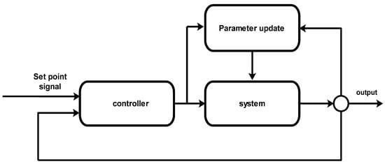
Figure 6.
Block diagram of adaptive MPC.
Due to the computational complexity, the convergence rate of the commonly adopted technique RLS for online parameter estimation is slow, so in the proposed work, we adopted a new technique, multi-innovative recursive least square algorithm, which measures the parameters more quickly, so the performance of the model is also increased, which give a better design for online parameter estimation of the time-varying system [20,21,22].
In the literature review, we consider different models of time series model prediction in which every model carries different techniques for linear and nonlinear systems, a few models are for linear systems, and some are for nonlinear systems, but they have some restrictions and limits for input, output, and control variable constraints [3]. In the proposed modeling scheme, we used a non-minimal state space model, which can capture the dynamics of the time-varying system the future parameters are identified through RLS algorithm, and quadratic optimization strategy is used for the constraints on input, output, and control variable [5]. For time, varying system the model plays an important role in the controller pre-performance [23]. A badly design model cannot generate a good estimate for the future trajectory. In the proposed work, we used an ARMAX model, which is most suitable than the ARX model and for parameter estimation, the RLS algorithm is used [5]. A lot of techniques are used for online and offline parameter estimation of LTI and time-varying. For online parameter estimation of the time-varying system, the RLS algorithm is the most suitable technique, but the convergence for parameter estimation is a little slow for time-varying system so we will use a new technique called multi-innovative recursive algorithm, which is faster than the commonly adopted RLS algorithm. With the fast parameter estimation tracking the performance of the model is also enhanced.
For single-input single-output (SISO) time-varying system, the model can be presented as in Equation (28).
where u(k) is the manipulated input to the system at time k, y(k) is the output at time k, and is the state vector by applying the difference equation, the above equation can be represented by the following:
The next states and the output can also be calculated with recursive least square algorithm. In compact form, the difference equation of the can be represented as
where
Now
where can be computed with commonly used RLS technique. is the output at time and is the input at time let the output can be find in the form of regression vector by the following:
where can be predicted with the commonly used (RLS) technique.
3.1. Online Parameter Estimation
In offline or batch processing identification, data up to some duration like t = N are first collected and then model parameters are calculated but in our proposed online or recursive identification model the parameters are required to be identified for every time t. A common control problem in the process industry where the plant dynamics changing quite significantly from one operating point to another operation points that is why the online parameter estimation is required to control the plant to obtain the desire response, the online parameter estimation problem gets much harder when there are high number of estimated parameters.
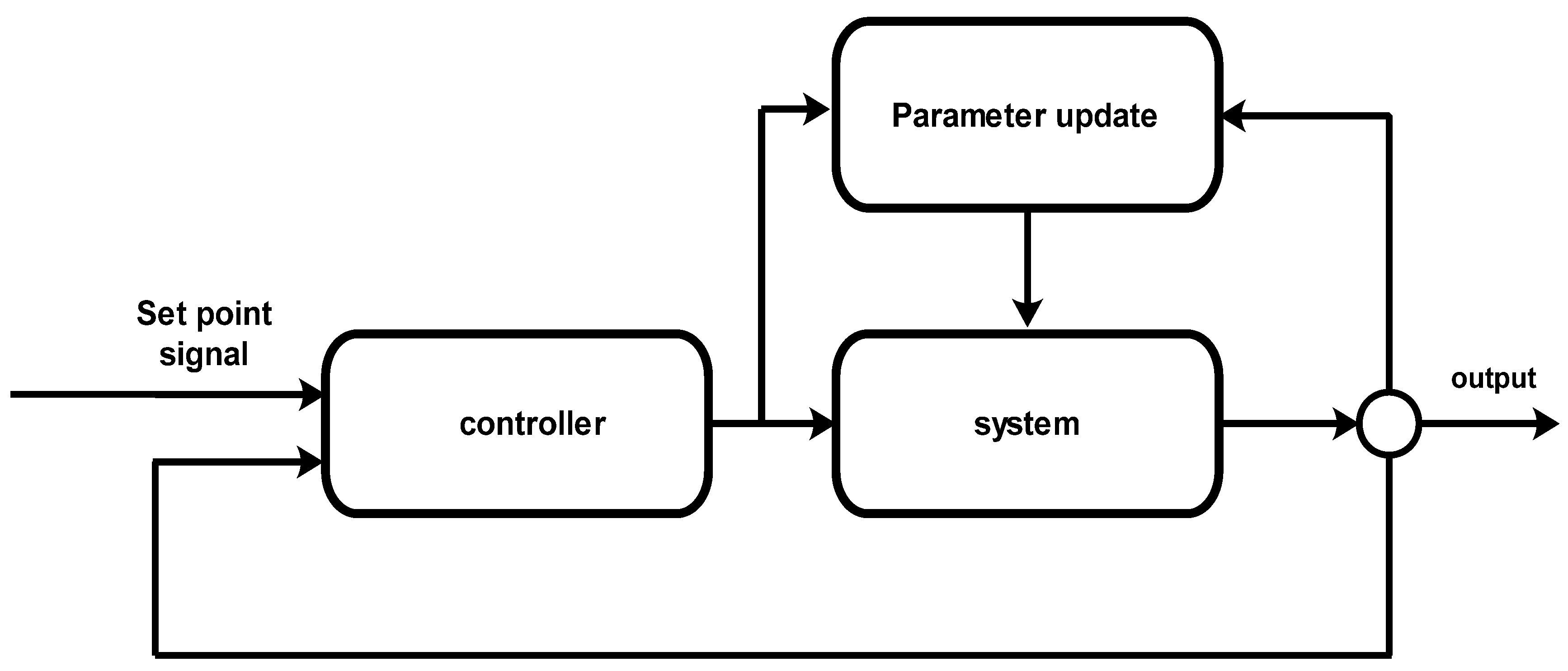
There are a lot of techniques for online parameter estimation such as RLS, MIRLS, stochastic gradient method, all these techniques have some advantages and drawbacks, it is more important that memory and the time required for computation do not increase with t. in the proposed work, we used the MIRLS algorithm due to its fast convergence rate and high efficiency. The block diagram of the online parameter estimation design is shown in Figure 7, where r is the reference signal, u is the input, and y is the output of the plant.
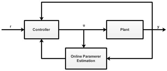
Figure 7.
Block diagram of online parameter estimation.
3.2. MIRLS
Multi-innovation recursive least square technique is used to increase the efficiency and convergence rate of the algorithm. The MIRLS algorithm can be presented as follows:
where , , and are the innovation vectors, is the input vector, and is the covariance matrix.
3.3. Parameter Estimation with Constraint
When there is a limitation on the control signal, input, or output signal then the system does not give the desired response, in the presence of constraint the closed-loop response of the system deteriorates to handle such constraint we apply the constraint control techniques [24]. Before discussing the constraint, handling technique consider a system without constraints and check the response of the system k. Consider a mathematical model of the system as follows:
From the given state we can predict the future state variable up to Np, Np is the length the prediction horizon, let the future state variables denoted by , and the future control moves by . After the augmented state space model as discussed, the relation between the state vector and control vector can be defined in such form [25].
where
where is a diagonal matrix of the output equation of the state space [22]. Let the set point trajectory of the future output is observed with a vector
where is the set point of the cost function, which can be chosen as .
The dimension of is equal to the dimension of [25]. From the above formulation, we can predict the future moves of the control variable future state vector and future output vector, but in the presence of constraints on the control variable, input variable, and output variable the performance of the MPC deteriorate. To handle this constraint, we may need an optimization formulation to enhance the performance of the MPC. In the proposed work, we apply the Hildreth quadratic optimization technique, which clearly handles these constraints.
Hildreth programming is a row-action technique for quadratic programming [26]. It is a very useful algorithm for solving large scale quadratic programs and it can also handle equality and inequality constraint problem [27].
Let us suppose we have a cost function with some constraint, and we want to minimize this function.
such that
where a, b, g, h, m, and k, are some real numbers. By using Hildreth quadratic programming we can write cast function as
In the proposed work we used Hildreth quadratic technique to handle such constraints.
4. Results and Discussion
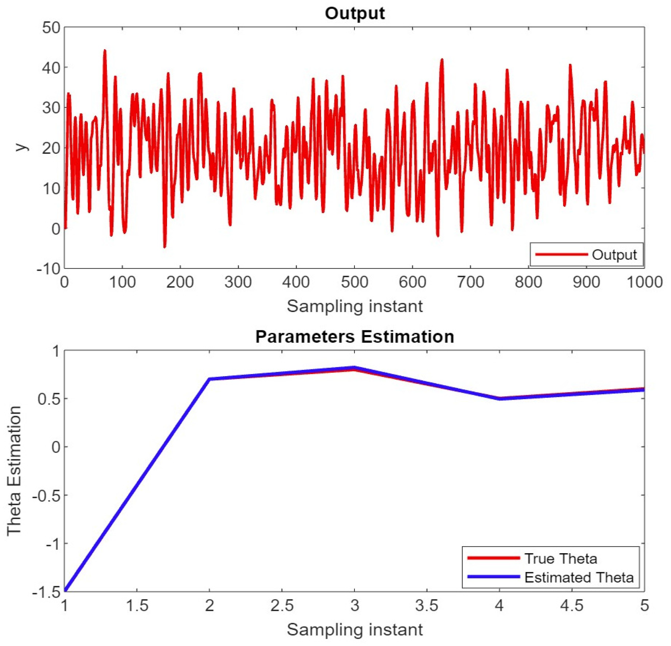
We successfully estimated the ARMAX model parameters, and the simulation results are shown in Figure 8. We used the same version of MATLAB to simulate the result of the algorithm for parameters .
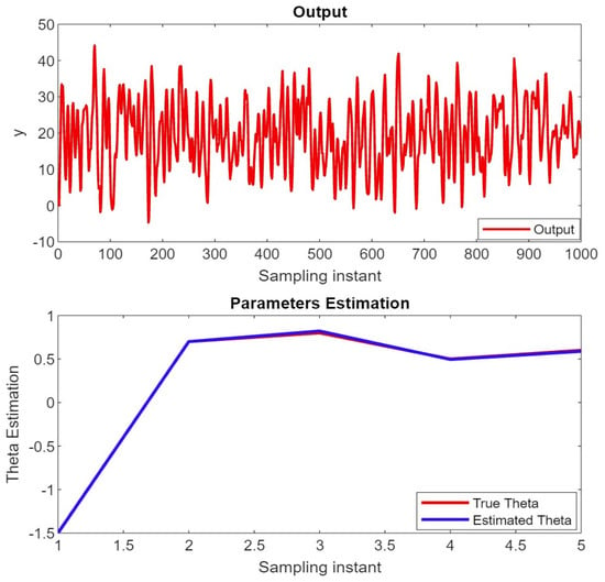
Figure 8.
Parameters estimation vector.
These parameters, [, ], [, ], and , represent the coefficients of the model, which indicate the effect of past output on the current output, the effect of output on the past input, and the influence of the current output on the input, respectively, our simulation results shows that our model estimated these parameters correctly. These parameters are used to build the mathematical model of the system which show the system’s symmetric behavior for unknown parameters estimation.
4.1. Parameter Estimation with MIRLS and Sensitivity Analysis
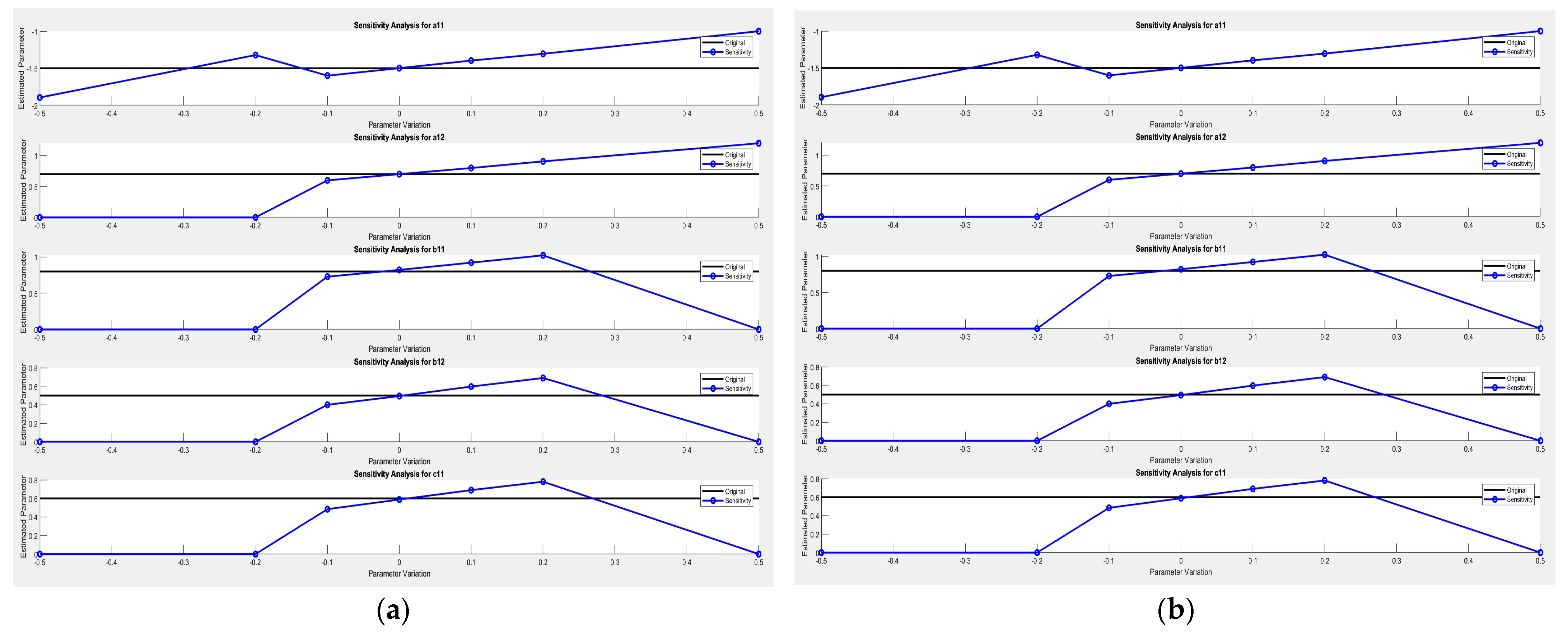
We tested the model with the parameters for p = 1, and p = 2. The results are shown in Figure 9, where p is the length of the innovation.
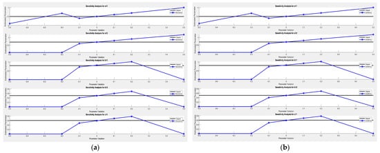
Figure 9.
Sensitivity analysis.
Figure 9a shows the model response for p = 1 and Figure 9b shows the response for p = 2. It illustrates that the MIRLS algorithm is more efficient and fast in terms of parameter estimation. By changing the length of the p, the desired estimation results can be achieved.
The system parameters, a11, a12, b11, b12, and c11, have been adjusted to different values. The new values are chosen to provide a closer alignment between the estimated parameter values and the original parameter values for sensitivity analyses, as shown in Figure 9a,b. Finding optimal parameter values for a specific need may require further experimentation and adjustment. Consider refining the parameter variations or exploring different parameter values to achieve the desired level of sensitivity and alignment in the sensitivity analysis results.
4.2. Simulation Result of Adaptive MPC
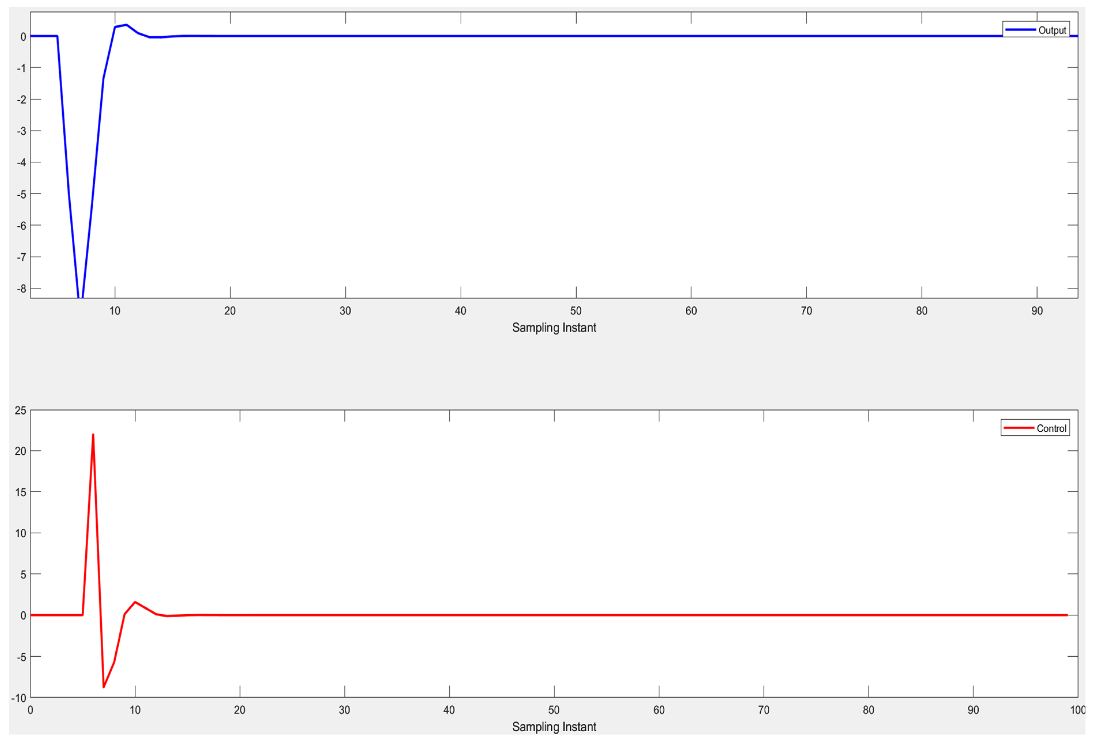
Systems output with the given parameters and the control signal is shown in Figure 10.
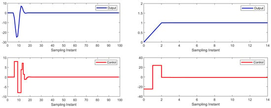
Figure 10.
NMSS MP controller.
From the simulation result, we can analyze that the controller is tracking the output of the system symmetrically and setting the control moves accordingly.
4.3. Adaptive MPC with Constraints Simulation Results
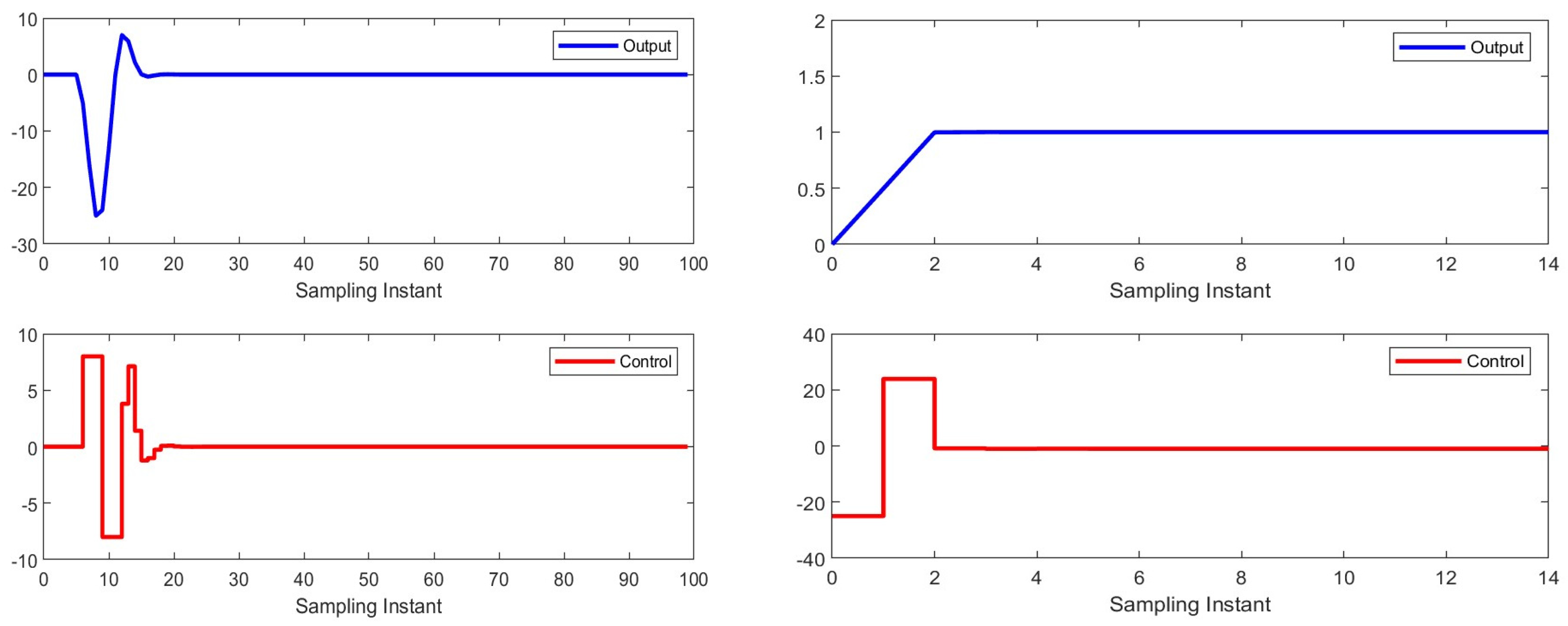
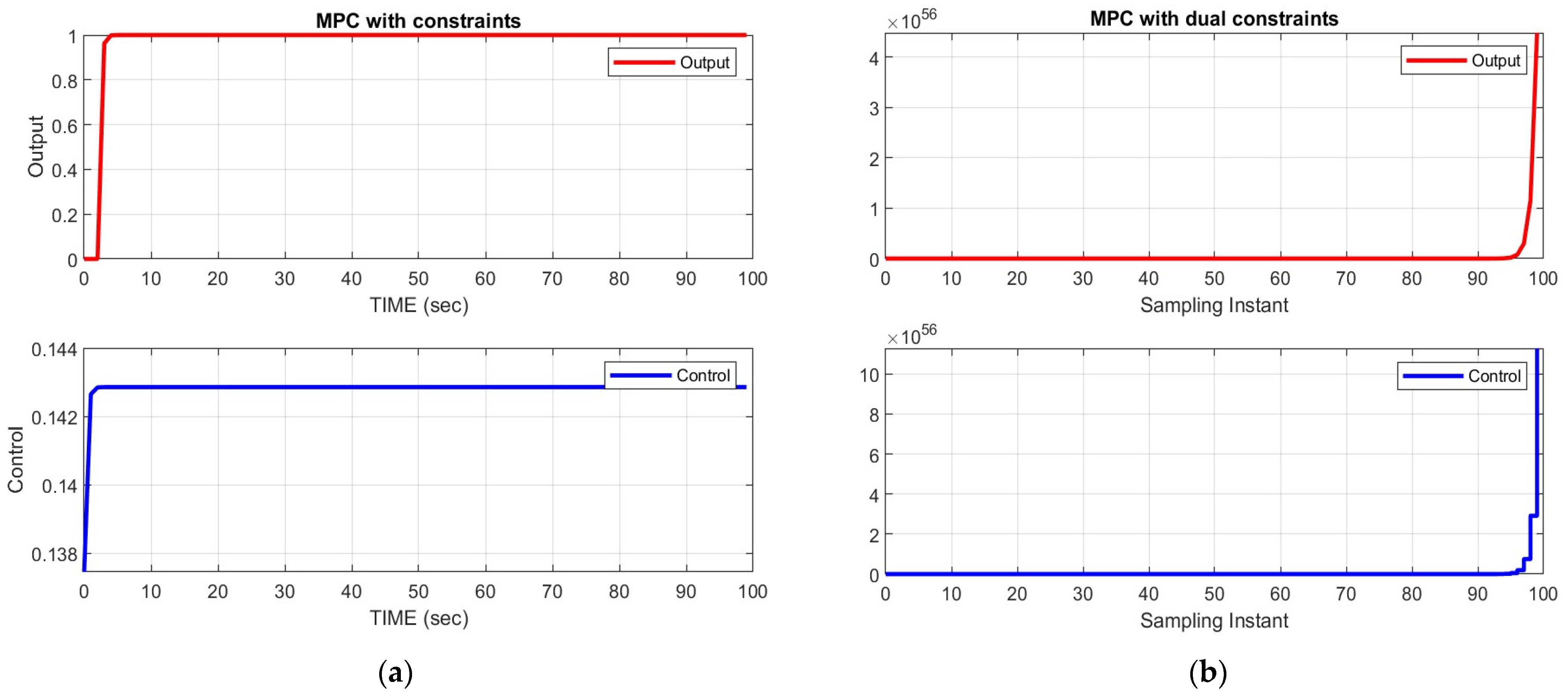
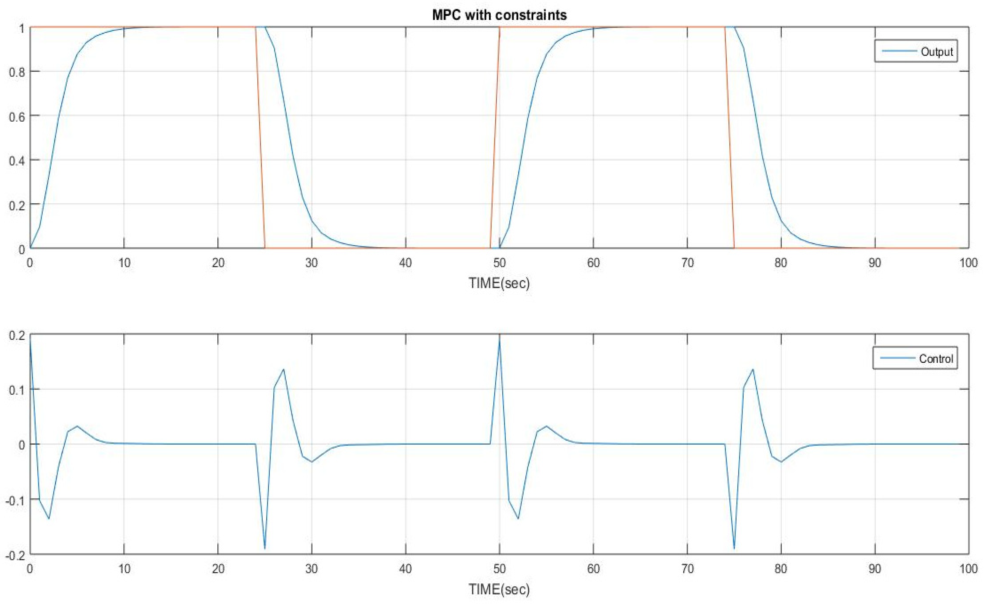
In the proposed work, we used the parameters of a plant model of an industrial weight feeder, which consists of a motorized gate control, to regulate the flow of weight feed. The objective of the proposed work is to design a controller to maintain the flow of the weight feeder, the proposed controller is tested on a system model to track the control move and set the input accordingly, as shown in Figure 11. Figure 12a shows the behavior of the output and control signal for a single constraint on the input, while Figure 12b shows the response of the system in the presence of dual constraints, both on the input and the output.
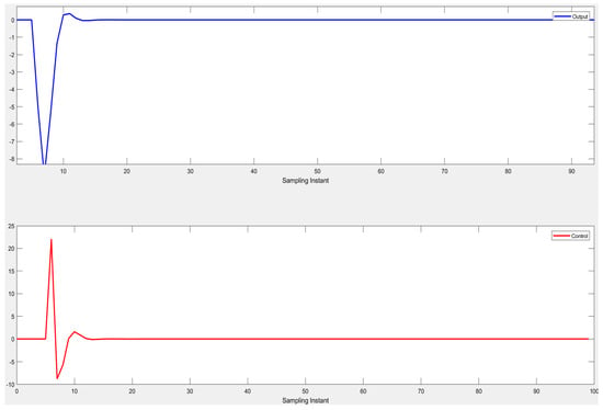
Figure 11.
Adaptive MPC with constraint.

Figure 12.
Adaptive MPC with single and dual constraints.
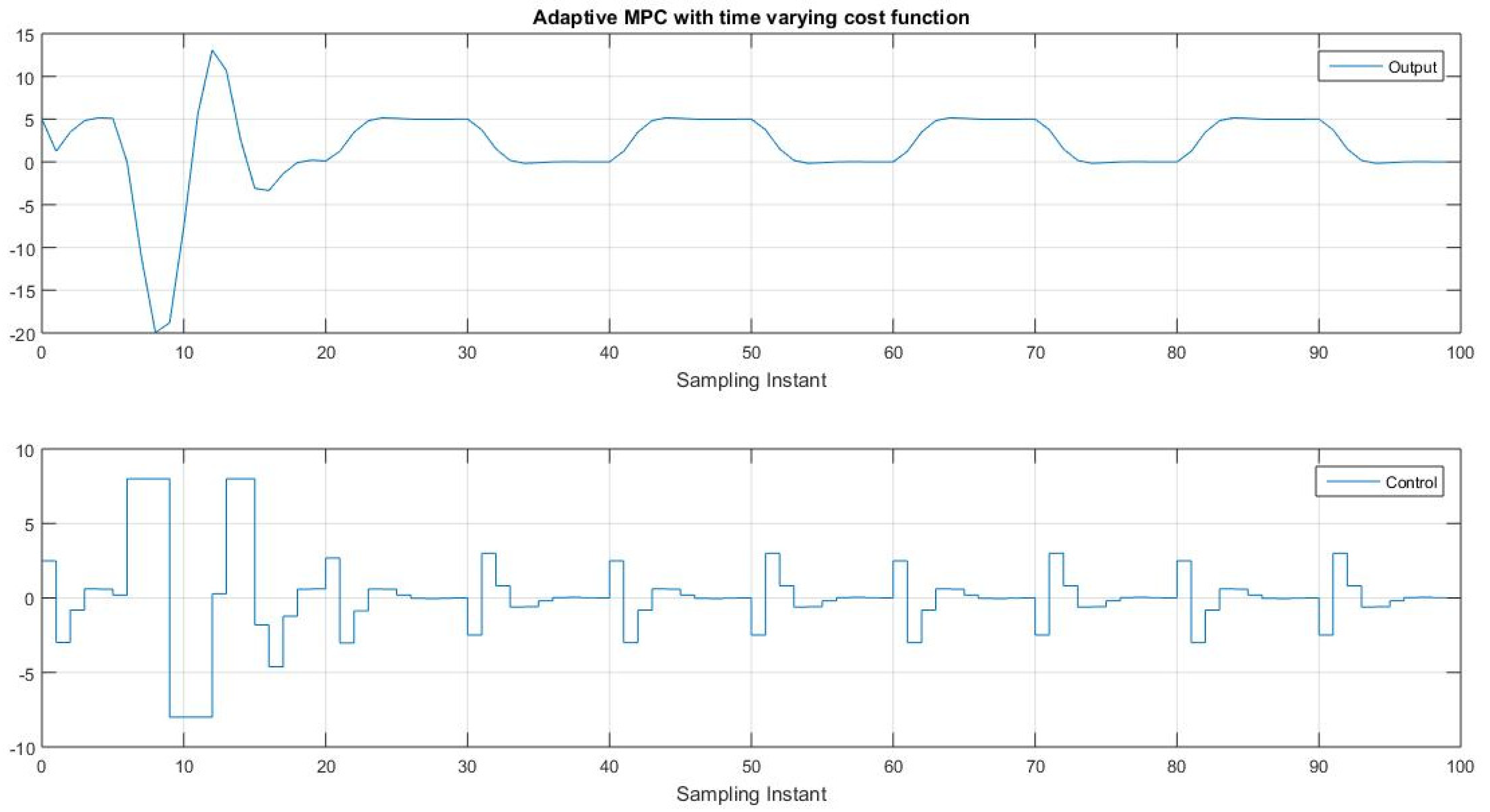
Figure 13 and Figure 14 represent the output and control signal of a time-varying model predictive controller with dual constraints. The system being controlled is a double integrator with the transfer function discretized with a time difference of one. In the graph, the top subplot displays the output signal, while the bottom subplot shows the control signal. The x-axis represents time, y-axis represents the corresponding values of the output and control and orange line in the graph shows the presence of constraints.
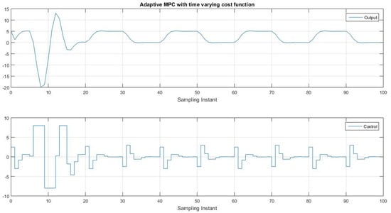
Figure 13.
AMPC with time varying cost function.
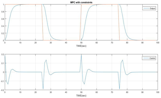
Figure 14.
AMPC with time varying cost function and constraints.
The control signal is shown in the bottom subplot, indicating the applied control action to symmetrically regulate the system. The control input follows the changes required to generate the desired output signal while considering the constraints imposed on the control horizon. The control signal satisfies the constraints and maintain the stability as well as performance of the system symmetrically.
The plot showcases the effectiveness of the time-varying adaptive model predictive controller, which tracks the desired output, and sets the control move accordingly, even when the system parameters change over time. It demonstrates the ability of the controller to adapt to dynamic conditions and enforce constraints while achieving the desired control objectives to minimize the input.
5. Conclusions and Future Work
The simulation and experimental results validate the effectiveness of an online parameter estimation and adaptive control method based on non-minimal state space. This method eliminates the need for a state observer, potentially reducing the sensitivity of the controller to model mismatch issues compared to the observer-based minimal state equivalent. In the proposed work, we present different techniques for parameter estimation of a SISO time-varying system, which integrate the controller design and enhance the efficiency and convergence rate of the parameter estimation. The proposed design minimizes the parameter estimation error variance and maximizes the efficiency of the system by changing the length of the innovation vector, the simulation results also show the improved parameter estimation of the time varying system in terms of convergence rate and efficiency, and the NMSS-AMPC can symmetrically handle the constraints very effectively. We can extend our design for a multiple-input multiple-output (MIMO) system to predict the future control moves of a time-varying system.
Author Contributions
Conceptualization, Z.U.R. and H.M.; methodology, Z.U.R. and H.M.; supervision, Z.U.R. and H.M.; investigation, Z.U.R. and M.A.A.K.; writing—original draft preparation, Z.U.R. and M.A.A.K.; writing—review and editing, Z.U.R., M.A.A.K. and M.R. All authors have read and agreed to the published version of the manuscript.
Funding
This research work was funded by the National Key Research and Development Plan of China (2018AAA0101000) and the National Science Foundation of China (62076028).
Data Availability Statement
Not applicable.
Acknowledgments
The authors sincerely thank the associate editor and the anonymous reviewers for their valuable suggestions and comments that improved the quality of our work.
Conflicts of Interest
The authors declare no conflict of interest.
References
- Sun, Z.; Qin, S.J.; Singhal, A.; Megan, L. Performance monitoring of model-predictive controllers via model residual assessment. J. Process Control 2013, 23, 473–482. [Google Scholar] [CrossRef]
- Karra, S.; Shaw, R.; Patwardhan, S.C.; Noronha, S. Adaptive Model Predictive Control of Multivariable Time-varying Systems. Ind. Eng. Chem. Res. 2008, 47, 2708–2720. [Google Scholar] [CrossRef]
- Zhu, Y. System identification for process control: Recent experience and outlook. Int. J. Model. Identif. Control 2009, 6, 89–103. [Google Scholar] [CrossRef]
- Bingül, Ö.; Yıldız, A. Fuzzy logic and proportional integral derivative based multi-objective optimization of active suspension system of a 4×4 in-wheel motor driven electrical vehicle. J. Vib. Control 2023, 29, 1366–1386. [Google Scholar] [CrossRef]
- Heirung, T.A.N.; Foss, B.; Ydstie, B.E. MPC-based dual control with online experiment design. J. Process Control 2015, 32, 64–76. [Google Scholar] [CrossRef]
- Ljung, L. System identification. In Signal Analysis and Prediction; Birkhäuser Boston: Boston, MA, USA, 1998; pp. 163–173. [Google Scholar]
- Kesson, J. MPCtools 1.0: Reference Manual; Department of Automatic Control, Lund University: Lund, Sweden, 2006. [Google Scholar]
- Duan, H.; Jia, J.; Ding, R. Two-stage recursive least squares parameter estimation algorithm for output error models. Math. Comput. Model. 2012, 55, 1151–1159. [Google Scholar] [CrossRef]
- Friedland, B. Control System Design: An Introduction to State-Space Methods; Courier Corporation: Chelmsford, MA, USA, 2012. [Google Scholar]
- Wang, L.; Young, P.C. An improved structure for model predictive control using non-minimal state space realisation. J. Process Control 2006, 16, 355–371. [Google Scholar] [CrossRef]
- Junsheng, C.; Dejie, Y.; Yu, Y. A fault diagnosis approach for roller bearings based on EMD method and AR model. Mech. Syst. Signal Process. 2006, 20, 350–362. [Google Scholar] [CrossRef]
- Gaines, B.R. System identification, approximation, and complexity. Int. J. Gen. Syst. 1977, 3, 145–174. [Google Scholar] [CrossRef]
- Sharma, T.C.; Panu, U.S. Analytical procedures for weekly hydrological droughts: A case of Canadian rivers. Hydrol. Sci. J.–J. Des Sci. Hydrol. 2010, 55, 79–92. [Google Scholar] [CrossRef]
- Ström, K.J.; Eykhoff, P. System identification—A survey. Automatica 1971, 7, 123–162. [Google Scholar] [CrossRef]
- Kersting, S.; Buss, M. Direct and indirect model reference adaptive control for multivariable piecewise affine systems. IEEE Trans. Autom. Control 2017, 62, 5634–5649. [Google Scholar] [CrossRef]
- Toplis, B.; Pasupathy, S. Tracking improvements in fast RLS algorithms using a variable forgetting factor. IEEE Trans. Acoust. Speech Signal Process. 1988, 36, 206–227. [Google Scholar] [CrossRef]
- Fedorov, V.V.; Leonov, S.L. Parameter estimation for models with unknown parameters in variance. Commun. Stat.-Theory Methods 2004, 33, 2627–2657. [Google Scholar] [CrossRef]
- Ding, F.; Liu, P.X.; Liu, G. Auxiliary model based multi-innovation extended stochastic gradient parameter estimation with colored measurement noises. Signal Process. 2009, 89, 1883–1890. [Google Scholar] [CrossRef]
- Taylor, C.J.; Chotai, A.; Young, P.C. State space control system design based on non-minimal state-variable feedback: Further generalization and unification results. Int. J. Control 2000, 73, 1329–1345. [Google Scholar] [CrossRef]
- Shouche, M.; Genceli, H.; Premkiran, V.; Nikolaou, M. Simultaneous Constrained Model Predictive Control and Identification of DARX Processes. Automatica 1998, 34, 1521–1530. [Google Scholar] [CrossRef]
- Chen, H.; Gong, Y.; Hong, X. Adaptive modelling with tunable RBF network using multi-innovation RLS algorithm assisted by swarm intelligence. In Proceedings of the 2011 IEEE International Conference on Acoustics, Speech and Signal Processing (ICASSP), Prague, Czech Republic, 22–27 May 2011; pp. 2132–2135. [Google Scholar] [CrossRef]
- Sirmatel, I.I. Adaptive Model Predictive Control of Constrained Multiple-Input Multiple-Output Systems and Its Application to the Quad Tank System. Master’s Thesis, ETH-Zürich, Zürich, Switzerland, 2014. [Google Scholar]
- Rathouský, J.; Havlena, V. MPC-based approximate dual controller by information matrix maximization. Int. J. Adapt. Control Signal Process. 2013, 27, 974–999. [Google Scholar] [CrossRef]
- Gorman, J.; Hero, A. Lower bounds for parametric estimation with constraints. IEEE Trans. Inf. Theory 1990, 36, 1285–1301. [Google Scholar] [CrossRef]
- González, A.H.; Perez, J.M.; Odloak, D. Infinite horizon MPC with non-minimal state space feedback. J. Process Control 2009, 19, 473–481. [Google Scholar] [CrossRef]
- Hildreth, C. A quadratic programming procedure. Nav. Res. Logist. Q. 1957, 4, 79–85. [Google Scholar] [CrossRef]
- Herman, G.T.; Lent, A. A family of iterative quadratic optimization algorithms for pairs of inequalities, with application in diagnostic radiology. In Mathematical Programming in Use; Springer: Berlin/Heidelberg, Germany, 1978; pp. 15–29. [Google Scholar] [CrossRef]
Disclaimer/Publisher’s Note: The statements, opinions and data contained in all publications are solely those of the individual author(s) and contributor(s) and not of MDPI and/or the editor(s). MDPI and/or the editor(s) disclaim responsibility for any injury to people or property resulting from any ideas, methods, instructions or products referred to in the content. |
© 2023 by the authors. Licensee MDPI, Basel, Switzerland. This article is an open access article distributed under the terms and conditions of the Creative Commons Attribution (CC BY) license (https://creativecommons.org/licenses/by/4.0/).

