Deep Learning Approach to Source Localization of Electromagnetic Waves in the Presence of Various Sources and Noise

Abstract

In this paper, the 3D localization and signal enhancement problem of a source in a noisy environment is addressed using an antenna array to ensure symmetry in communication engineering. The use of machine-learning-dependent convolutional recurrent neural networks (CRNN) and a minimum variance distortionless response (MVDR) beamformer for the localization of the source is developed. Furthermore, to ensure the adaptability of the signal enhancement module during deployment in a new environment or in new conditions, the training of a meta-learning model is conducted. At first, during the localization, the direction of arrival (DoA) estimation in both azimuth and elevation angles is generated. This is generated in a noisy three-dimensional plane and multi-source signal. Employing the DoA estimates, the MVDR is used for the enhancement of the signal source. Verifying the proposed method in the presence of mutual coupling, the two scenarios in communication engineering were simulated using a ray-tracing tool in the form of a real-world problem towards enhancing a signal source in a noisy environment and in the presence of various sources. The results obtained demonstrate how the proposed method outperforms the machine learning and parametric methods. In addition, the trained meta-learning model is employed to demonstrate how the proposed method is adaptable to any environment and still maintains an appreciable quality performance index after retraining with few data. Finally, the results obtained are motivating enough for the practical application of the proposed method.

1. Introduction

Source localization is a crucial topic in security [1], autonomous driving [2,3], radar, and mobile communications [3]. Source localization finds applications in 3D (three-dimensional) space, including signal tracking and detection, beamforming, and robotic navigation [2,4]. In communication engineering, direction of arrival (DoA) estimation is one of the key symmetrical factors in the design of communication links.

DoA of single and more active sources is employed to steer the directivity pattern of antenna arrays in intelligent systems [2] or wireless communications [4,5,6]. The use of an antenna array for source localization enhances the signal. In addition, the estimated DoA is employed by the beamformer for signal enhancement [4].

DoA estimation of a single source is contained in the overall technical procedure for source localization, where a particular assignment computes the plane of the active source regarding the antenna array configuration. DoA estimation methods are grouped into two classes: The first is the machine-learning-inspired methods, which use and train machine learning algorithms (such as deep learning) for the estimation of the source’s direction and position [7,8,9,10,11,12,13,14,15,16,17]. The second class is the parametric methods, such as the ones that use MUSIC (multiple signal classification), MUSIC group delay, generalized cross-correlation (GCC), adaptive eigenvalue decomposition, estimation of subspace rotational in variance technology (ESPRIT) [18], and SRP (steered-response power) [19].

Present growths in machine learning made the model’s training and validation possible and produced the ability to perform signal localization in noisy environments, even with multi-source signals. Recently, Adavanne et al. [7] employed convolutional recurrent neural networks to detect and localize imbricating sources. On the other hand, no noisy data are considered, and no signal enhancement is conducted because the study is tailored towards signal detection. This paper uses a machine-learning algorithm for the purpose of localization and signal enhancement in a noisy multi-source environment. Presently, there are various deep neural network-dependent methods with various geometries of array and input features adopted. Furthermore, the convolutional neural network having a spectrum of phases as input from linear arrays has been employed for the signal source’s azimuth angle estimation [9,10]. In addition, fully connected networks were developed in [10,11,12] for azimuth angle estimation [10,11,12,13], employing circular arrays to estimate the azimuth angle in multi-source cases. In addition, both elevation and azimuth angles are estimated by using the spectrum and magnitude of signals using the structure of CRNN [12]. A temporal convolutional network [13] was employed for the enhancement of the work in [14]. Finally, the features of the generalized cross-correlation were employed in [12,15,16,17,18,19] to conduct regression on the elevation and azimuth angles.

Achieving the directional transmission or reception of signal via antenna arrays is known as beamforming. Spatial filtering uses and produces the knowledge that those electromagnetic waves at perpendicular angles are affected by useful interference, and others are affected by harmful interference. The beamformer finds application in communications, radar, and vehicular technology. An antenna beamforming array is formulated to be more active from one or more particular directions against the signals originating from other directions. There are already designed beamformers in the literature, such as minimum variance distortionless response (MVDR) [20], linearly constrained minimum variance (LCMV) [21], and delay and sum (DAS) [22]. In the delay and sum beamformer, all the received signals originating from one direction are summed and aligned collectively using the delay to leading signals. Conversely, DAS does not consider the associated noise with the received signals. The linearly constrained minimum variance beamformer employs a weighted filter aiming at reducing the output signal received via the consideration of linear constraints modeled to reconstruct the wanted signal filtering the unwanted signals where the DoA of wanted and unwanted signals are known. The minimum variance distortionless response beamformer is a special scenario of a linearly constrained minimum variance beamformer where it attempts to minimize signals arriving from all directions and protecting the wanted signals, provided the signal remains undistorted.

Meta-learning makes small-shot learning possible, aiming to train models on various learning assignments in such a way that it exhibits good performance on other learning assignments employing few data or samples and iterations of the training [23]. This method is a good candidate where there is a scarcity of training datasets or where there is difficulty in getting datasets, or a case where the model is required to adapt to another scenario. The method is not difficult to manipulate.

Meta-learning has been employed mostly in computer vision [24,25] or language processing [26,27]. However, few studies have been reported on electromagnetic waves. Both [28] and [29] employed a small number of shot learning methods for recognizing and detecting multiple label signals. Hence, the DoA estimation problem in electromagnetics with a small number of shots employing meta-learning has not been seriously researched convincingly.

Meta-learning methods work on various approaches where the algorithms are trained via the distance-based prediction law [30,31], model-dependent approaches where a predictor with parameter is trained towards estimation of the model parameters [32,33], or gradient-dependent approaches employing gradient descent for the adaptation of the parameters of the model [34]. The last method performs well, compared to other approaches that do not depend on the structure of the model, and it’s useable for regression, reinforcement, and classification learning, which are part of the model agnostic meta-learning (MaMl) scheme [34].

The operation of the meta-learning is presented here. Consider an equation defined by function $f_{\varphi }$ having $\varphi$ values; MaMl learns the values of initialization $f_{{\varphi }_0}$ from the overall assignment sampled from the source dataset (${\mathsf{{\rm T}}}_i\in {\mathrm{Ɗ}}_s)$ in such a way that the model performs well on identical assignments sampled from target dataset (${\mathrm{Ƭ}}_i\in {\mathrm{Ɗ}}_t)$ following the small gradient descent steps. The initial values have high sensitivity to the difference in a particular task ${\mathrm{Ƭ}}_i$, where few differences in values generate appreciable enhancements on the task’s loss function when changed in the gradient direction of such loss. The objective function of MaMl is finding the ${\varphi }_0$, as shown below [34]:

$${\varphi }_0=\underset{\varphi }{\min }\sum _{{\mathsf{{\rm T}}}_i}{\mathfrak{R}\mathsf{{\rm T}}}_i\left(f_{{\varphi }_i}\right)$$

(1)

The MaMl model begins by random initialization of the parameters of the model ($\varphi {=\varphi }_0$). In the process of individual iterations of meta-learning, the event of a series of tasks ${\mathsf{{\rm T}}}_i$ are employed for updating the values of the algorithm via gradient update (check Equation (2) of [34]).

$${\widehat{\varphi }}_i=\varphi -\alpha \times {\nabla }_{\varphi }{\mathfrak{R}\mathsf{{\rm T}}}_i\left(f_{{\varphi }_i}\right)$$

(2)

$\alpha$ represents the learning hyper-parameter, and $\mathfrak{R}$ denotes the loss function. After each iteration, the meta-optimization across each assignment is computed, giving the system parameter update [34]

$${\widehat{\varphi }}_i=\varphi -\beta \times {\nabla }_{\varphi }\sum _{{\mathsf{{\rm T}}}_i}\mathfrak{R}{\mathsf{{\rm T}}}_i\left(f_{{\widehat{\varphi }}_i}\right)$$

(3)

$\beta$ denotes the meta-step size. In addition, after all the iterations, ${\varphi }_0$ produces the output of the algorithm.

Moreover, the state-of-the-art (including parametric and machine-learning-based methods) have not considered localizing a specific source of interest amidst multiple sources and noise. As such, this paper looked into this gap by developing a machine-learning-based system to localize a particular source within various sources in a noisy environment. Therefore, the major innovations of this article are highlighted below.

(i)

A machine learning algorithm for the localization of a source of interest within a multi-source and noisy environment is proposed. The model training, validation, and testing are conducted on realistic data generated from a noisy environment;

(ii)

A signal improvement pipeline that mixes the source localization with array beamforming is developed. The pipeline is tested on the real data;

(iii)

The developed model and the pipeline are compared against two machine learning methods and popular parametric methods, such as SRP-PHAT and MUSIC.

2. Mathematical Formulation of Problem

Consider an M number of sources situated at a far field of the circular antenna array of N elements, then the received signal of each element $n_i$ in the time domain is given as

$$y_i(t)=\sum _{m=1}^M{s}_m(t-t_i{(d}_m))\ast h_{im}(t)+n_i(t)$$

(4)

where $s_m\left(t\right)$ represents the targeted source in time domain from direction $d_s=\left[x_s,y_s,z_s\right]\cong [{\theta }_s,{\varphi }_s]$, corresponding to the center of the antenna array. $t_i\left(d_m\right)$ and $h_{im}$ represent propagation delay and the impulse response from the m source to the $i$th antenna, respectively, and $n_i\left(t\right)$ denotes the additive white Gaussian noise at the element $n_i$. $h\left(t\right)$ depends on signal speed, c.

$$Y=\sum _{m=1}^M{S}_m\ast H_m+N=\sum _{m=1}^M{X}_m+N$$

(5)

where $Y=\left[y_1\left(t\right),y_2\left(t\right),\dots ,y_N\left(t\right)\right],$ $X=\left[s_1\left(t\right)\ast h_1\left(t\right),s_2\left(t\right)\ast h_2\left(t\right),\dots ,s_N\left(t\right)\ast h_N\left(t\right)\right],$ and $M=\left[m_1\left(t\right),m_2\left(t\right),\dots ,m_N\left(t\right)\right]$.

If the interest is a major source (MS: m = 1), then Equation (5) becomes

$$Y=X_{MS}+\sum _{m=2}^M{X}_m+N=X_{MS}+N_E$$

(6)

where $N_E\in {\mathbb{R}}^N$ merges other sources and additive Gaussian noise.

The goal is to perform the DoA estimation in elevation and azimuth planes ${(\widehat{\theta }}_s,{\widehat{\varphi }}_s)$, and for a specific array geometry, computing the antenna array steering vector $℮({\widehat{d}}_s,f)\in {\mathbb{C}}^N$ in the direction of the major source at a particular frequency f using

$$℮\left({\widehat{d}}_s,f\right)=[e^{j2\pi f{\tau }_1\left({\widehat{d}}_s\right)},e^{j2\pi f{\tau }_2\left({\widehat{d}}_s\right)},\dots ,e^{j2\pi f{\tau }_N\left({\widehat{d}}_s\right)}]$$

(7)

where ${\tau }_N\left({\widehat{d}}_s\right)\in \mathbb{R}$ represents the time delay between the $n$th element and its middle, which can be computed using

$${\tau }_N\left({\widehat{d}}_s\right)=\frac{r}{c}\times {\widehat{a}}_n\cdot {\widehat{a}}_s$$

(8)

where r represents the radius of the circular antenna array (CAA), c denotes the signal speed, ${\widehat{a}}_n$ represents the unit vector from the center of the CAA to the $n$th element direction $({\theta }_n,{\varphi }_n)$, and ${\widehat{a}}_s$ represents unit vector at the center of the CAA to the direction of the estimated source ${\widehat{d}}_s=({(\widehat{\theta }}_s,{\widehat{\varphi }}_s)$. The unit vectors are defined as

$$\begin{gathered} {\widehat{a}}_n={\widehat{a}}_x\sin \left({\theta }_n\right)\cos \left({\varphi }_n\right)+{\widehat{a}}_y\sin \left({\theta }_n\right)\sin \left({\varphi }_n\right)+{\widehat{a}}_z\mathrm{c}\mathrm{o}\mathrm{s}\left({\theta }_n\right) \\ {\widehat{a}}_s={\widehat{a}}_x\sin \left({\widehat{\theta }}_s\right)\cos \left({\widehat{\varphi }}_n\right)+{\widehat{a}}_y\sin \left({\widehat{\theta }}_s\right)\sin \left({\widehat{\varphi }}_s\right)+{\widehat{a}}_z\mathrm{c}\mathrm{o}\mathrm{s}\left({\widehat{\theta }}_s\right) \end{gathered}$$

(9)

In conclusion, both steering vector and MVDR beamforming can be employed to improve the EM wave ${\widehat{x}}_{MS}\left(t\right)$. The signal model is given in the following section.

3. Signal Model

The system framework, as shown in Figure 1, consists of two sections. First is the DoA estimation section using the machine learning (CRNN) method. The second one is the signal enhancement section using MVDR beamforming. The electromagnetic wave impinges the CAA from a specific azimuth and elevation angles ($\theta ,\varphi )$. The signal received is sampled and framed using the Hanning filter in the time domain. The short-time Fourier transform (STFT) on all frames is performed, and the result is input into the blocks.

3.1. DoA Estimation

Phase and magnitude per frequency bin are the features extracted. Normalizing the feature, the mean is subtracted and then calibrated to unit variance per feature. $x_s,y_s,$ $z_s$ are the unit sphere labels per feature based on the actual DoAs from

$$\begin{gathered} x_s=\cos \left({\varphi }_s\right)\mathrm{s}\mathrm{i}\mathrm{n}\left({\theta }_s\right) \\ {y}_s=\sin \left({\varphi }_s\right)\mathrm{s}\mathrm{i}\mathrm{n}\left({\theta }_s\right) \\ {z}_s=\mathrm{c}\mathrm{o}\mathrm{s}\left({\theta }_s\right) \end{gathered}$$

(10)

The feature input size against the model is $G\times F\times 2H,$ where $G=128$ represents the length of the sequence, $F=256$ denotes the positive frequency bins, and $H=7$ represents elements or radiators number. The features are input into the three layers of two-dimensional CNN of $Q=64$ filters $3\times 3\times 2H$. Following the individual layer of the 2D CNN, the activation function employed is ReLU [35], and the normalization of the result is conducted by batch normalization [36]. To reduce the input dimensionality, a max-pooling layer in the frequency domain is employed. The output of CNN is modified to a size $G\times 2H$ and put into two bi-directional RNN layers; $P=128$ units of GRU is employed for all layers with a tanh activation function. The two fully connected layers are then added. Layer one has P number of nodes and individuals having linear activation, and layer two has three nodes and tanh activation. The three nodes denote the estimated source direction (${\widehat{x}}_s,{\widehat{y}}_s,$ ${\widehat{z}}_s)$ of a unit sphere. The results of the last layer have $G\times 3$ shape. The angles of azimuth and elevation ${(\widehat{\theta }}_s,{\widehat{\varphi }}_s)$ for an input feature are computed using the mean of the output via

$${\widehat{\theta }}_s=\frac{1}{G}\sum _{i=1}^G\mathrm{a}\mathrm{r}\mathrm{c}\mathrm{t}\mathrm{a}\mathrm{n}(\frac{\sqrt{{{\widehat{x}}^2}_{si}+{{\widehat{y}}^2}_{si}}}{{\widehat{z}}_{si}})$$

(11)

$${\widehat{\varphi }}_s=\frac{1}{G}\sum _{i=1}^G\mathrm{a}\mathrm{r}\mathrm{c}\mathrm{t}\mathrm{a}\mathrm{n}(\frac{{\widehat{y}}_{si}}{{\widehat{x}}_{si}})$$

(12)

The Adam stochastic gradient approach is employed to calculate each layer kernel. The mean square errors that exist between the result of the model and the labels define the loss function employed for regression.

3.2. Beamforming

MVDR beamforming depends on data and requires wanted signal DoA information and noise statistics and signal interference. It reduces the noise and interference in all directions, apart from the wanted wave DoA.

$$\mathit{Y}\left(\omega \right)={\mathit{X}}_{MS}\left(\omega \right)+{\mathit{N}}_E\left(\omega \right)$$

(13)

here $\mathit{Y},$ $\mathit{X}$, and ${\mathit{N}}_E\in {\mathbb{C}}^N$. The outputs of the MVDR beamformer produce

$${\widehat{x}}_{MS}\left(\omega \right)={\mathit{F}}_{MVDR}^H\times \mathit{Y}\left(\omega \right)$$

(14)

where ^H is the Hermitian operation and ${\mathit{F}}_{MVDR}^H\in {\mathbb{C}}^N$ is the MVDR filter in the frequency domain and computed using the optimization equation

$$\begin{gathered} F_{MVDR}=\underset{F}{\mathrm{argmax}}{\mathit{F}}^H{\varphi }_{N_E{N}_E}\mathit{F} \\ s.t.{\mathit{F}}^H℮\left(d_s\right)=1 \end{gathered}$$

(15)

where $℮\left(d_s\right)$ denotes the steering vector for source direction $d_s=\left[{\theta }_s,{\varphi }_s\right],$ and ${\varphi }_{N_E{N}_E}{\mathbb{C}}^{N\times N}$ represents the covariance matrix of the noise. Solving Equation (15) generates the form [21,22]

$$F_{MVDR}=\frac{{{\varphi }^{-1}}_{N_E{N}_E}℮}{{℮}^H{{\varphi }^{-1}}_{N_E{N}_E}℮}$$

(16)

As depicted in Figure 1, the MVDR beamforming computes the coefficient of its filter depending on Equation (16) according to the DoA ${(\widehat{\theta }}_s,{\widehat{\varphi }}_s)$ estimate from the machine learning algorithm. In addition, an improved single channel datapoint, $\widehat{x}\left(t\right),$ is generated following the ISTFT (inverse STFT).

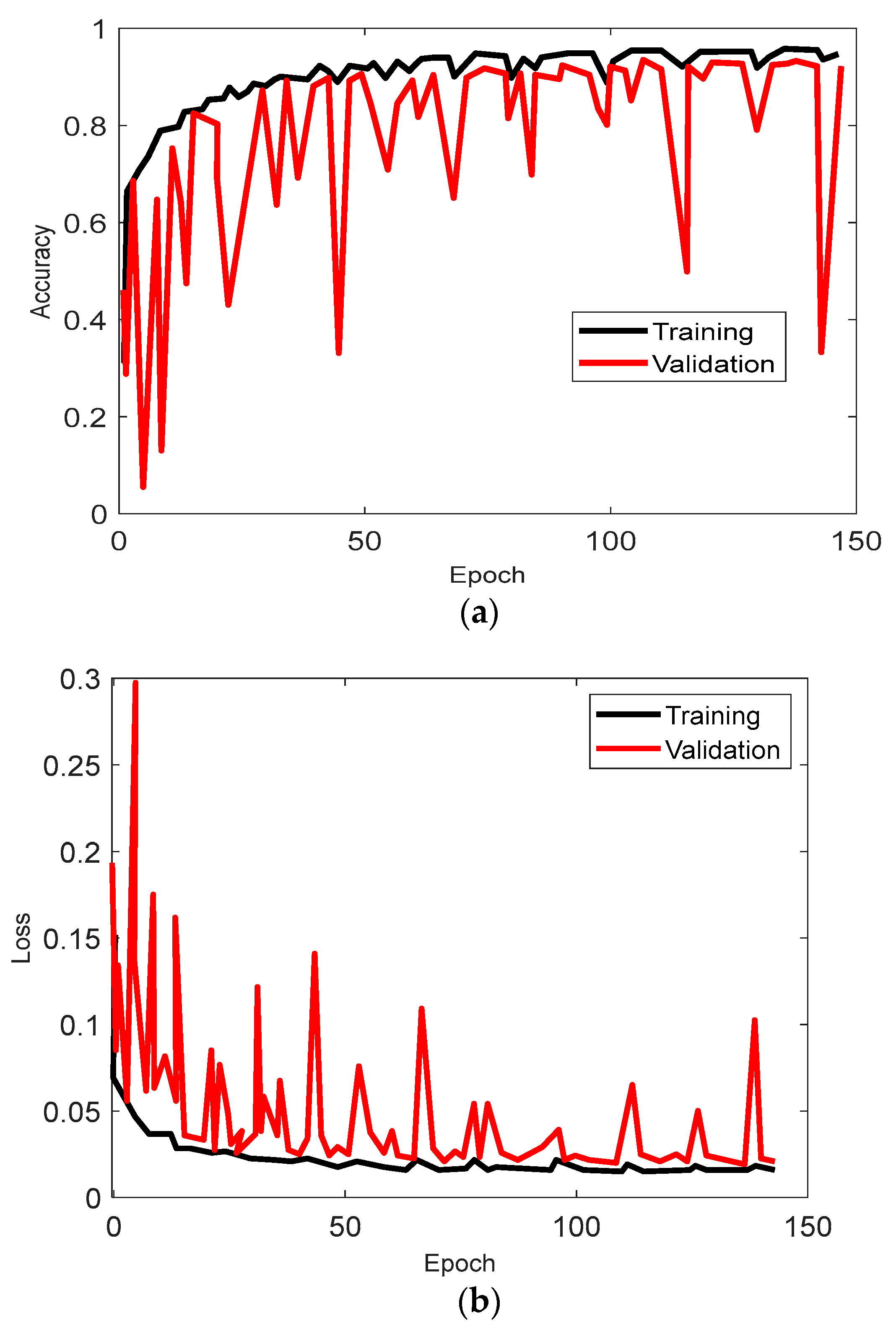
4. Dataset Generation and Numerical Analysis

The proposed method is analyzed against the CNN [12], FCN (fully connected network) [13], SRP-PHAT (steered response power phase transform) [19], and MUSIC algorithm [37] for DoA estimation in 2D space.

(A)

Dataset

The simulated data used in this article is electromagnetic radiation, which is obtained via a ray-tracing tool [38,39,40,41]. The two most popular communication scenarios (i.e., line-of-sight (LOS) and non-line-of-sight (NLOS)) in an urban region were simulated. The particular case used in this article is an urban area [42,43], and it is shown in Figure 2. The transmitter and receiver height is taken as 1.8 m. The multipath channel having four reflections and one diffraction is simulated using a 6 GHz carrier frequency. The ray-tracing simulation parameters employed for the generation of the dataset used in this work are presented in

Table 1. Ray-tracing tool parameters used for dataset generation.

Parameter	Value
Reflections	4
Diffraction	1
Transmission power	15 dB
Frequency	6 GHz
Antenna	Omnidirectional
$\mathrm{Permittivity}({\epsilon }_r$)	3.75
$\mathrm{Conductivity}(\sigma$)	0.137

. The number of simulated data for training, validation, and testing is 18,500. The positions of the main source are permutations of distances (4 m, 8 m, 12 m, 16 m) from the antenna array. Nineteen DoA azimuth angles were employed (0° to 180° with stepsize 10). Five DoA elevation angles were employed (70° to 110° with stepsize 10). Five signals from 10 sources are employed for the main signal. Random signals are taken from 14 sources from the telecommunication and signal processing dataset [44]. The dataset incorporates noise scenarios where the main source is with neighboring sources and noise. This helps in the training of the machine learning algorithm towards the identification of these signals and neglects their position, hence considering the main source.

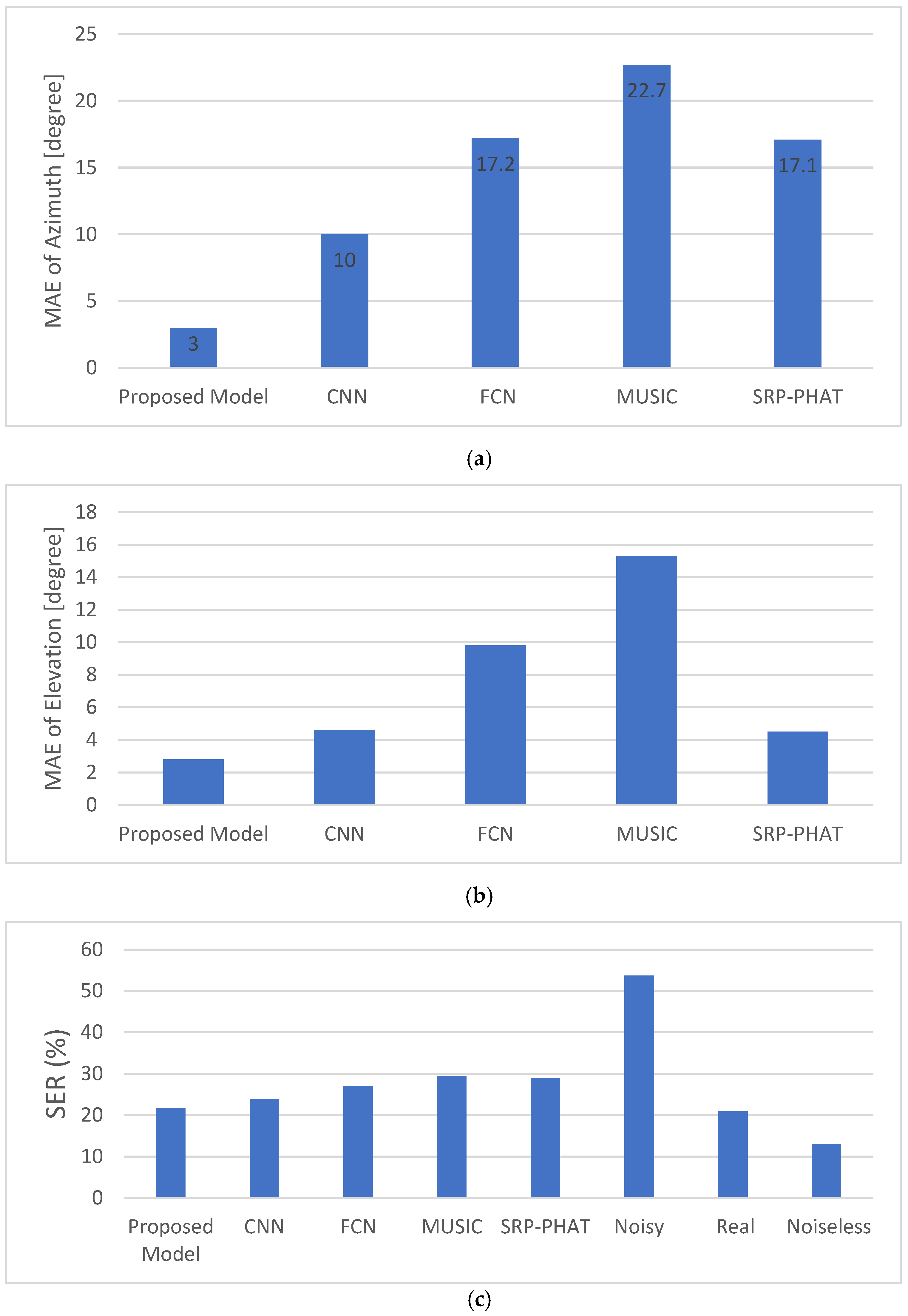
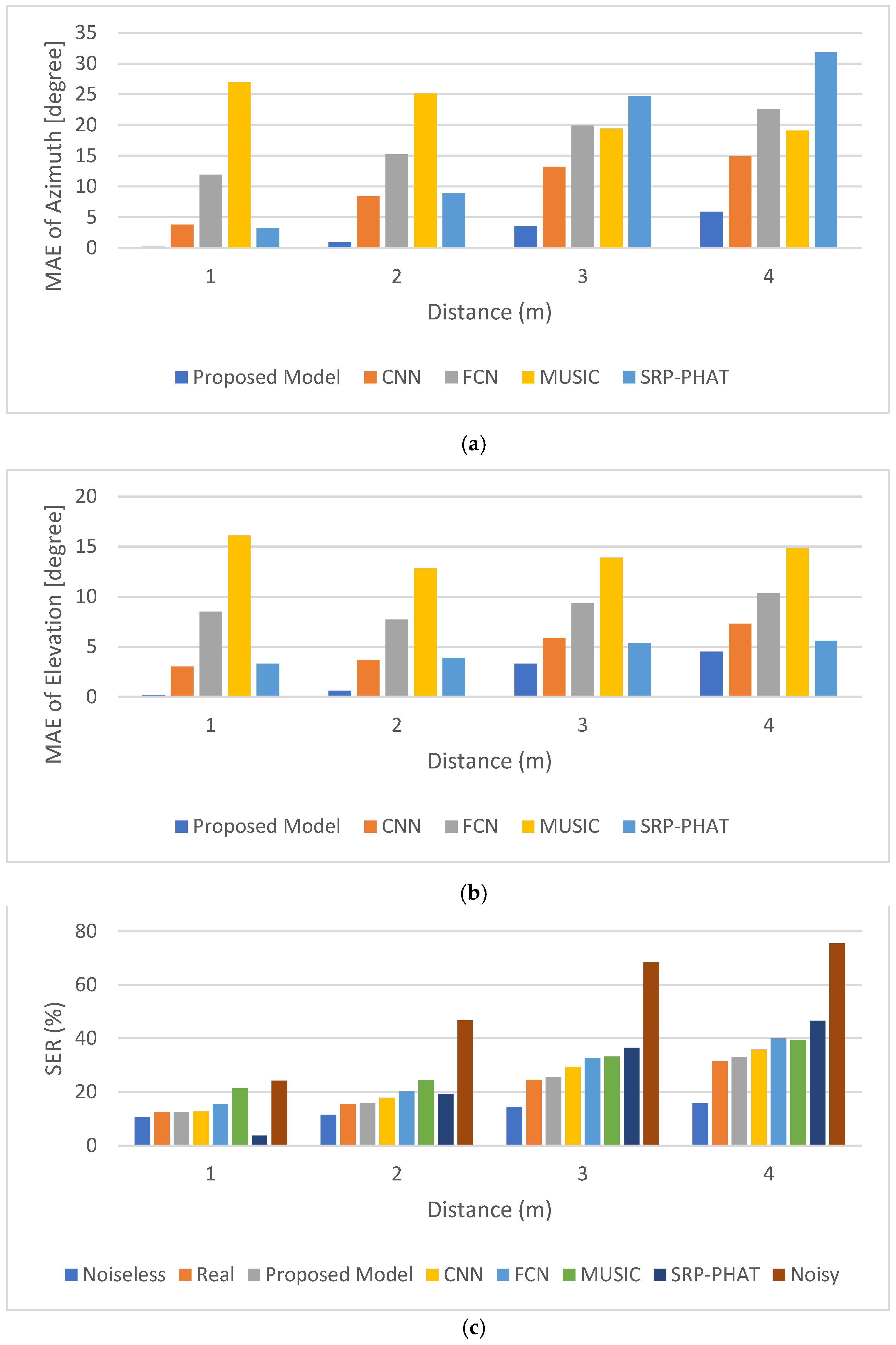
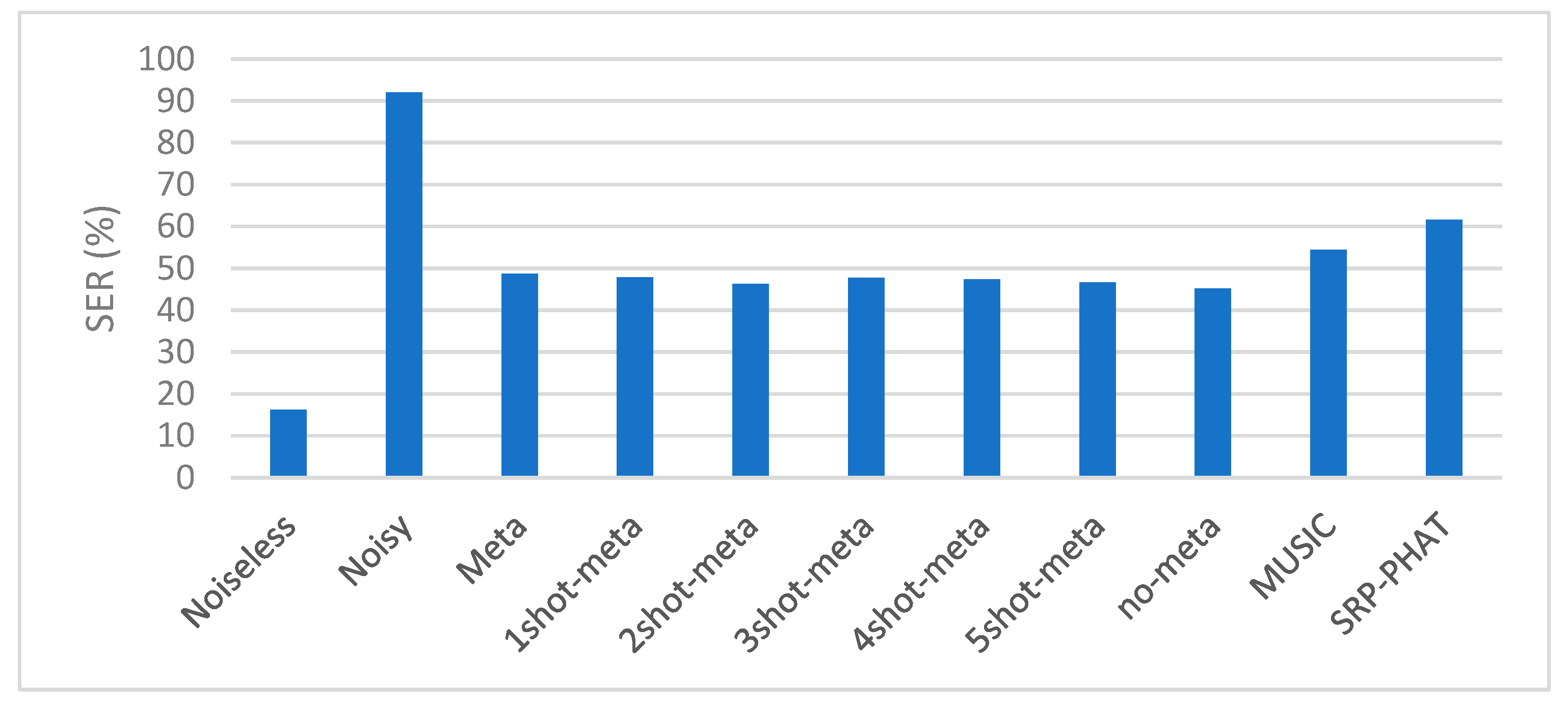
• (B) Numerical Experimental Results

The dataset is divided into three: 60% is used for training, 20% is used for validation, and 20% is used for testing. Figure 3 shows the accuracy and loss of the training and validation obtained for an asymptotic convergence using 143 epochs. When the epoch was set at 200, it was observed that the change was less than ${10}^{-4}$ for the 20 successive epochs.

The performance metrics for the DoA employed is the MAE (mean absolute error) using

$${MAE}_{\theta }=\frac{1}{M}\sum _{i=1}^M\left|{\theta }_i-{\widehat{\theta }}_i\right|$$

(17)

where M denotes the sample number and $\theta ,$ $\widehat{\theta }$ represent the true and predicted samples, respectively. Another performance metric used is the signal error rate (SER), computed in percentage [45]. SER is computed for different cases, such as the noisy, true, FCN/CNN, MUSIC/SRP-PHAT, and the proposed model.

The SER and MAE for the testing data for each distance and all kinds of noise are depicted in Figure 4. The developed approach performs better than the baseline parametric algorithms and the machine learning methods in both the elevation and azimuth angle estimation. The impact is shown in the SER results, where SRP-PHAT and MUSIC algorithms are around 7% bigger than the true dataset SER. In addition, both CNN and FCN are 4% and 7.2% higher, respectively. Meanwhile, the SER of the proposed method differs by just 0.6%.

The impact of the main source distance away from the CAA is depicted in Figure 5. The distance seriously affects the FCN and the SRP-PHAT. As the main source moved away from the antenna array, their estimated DoAs worsened. However, the proposed model is slightly affected in performance but still exhibits better performance than other methods. The impact of the MUSIC method is unclear, but it is clear that its performance is worse, particularly at lower distances. The CNN method exhibits good DoAs when the distance is short but degrades in performance as the main source moves away from the antenna array. Concerning the SER results, their behavior is impaired by distance as both the noisy and noiseless SER increases with distance. MVDR beamformer is affected by distance too. This is because the array directivity decreases with distance. In all cases, the proposed method outperforms other baseline methods.

The impact of the noises is shown in Figure 6. In SRP-PHAT and MUSIC methods, the number of active sources in each noise level is known, and the estimated angle that is nearest to the real main source is selected. In addition, two different models were trained towards the estimation of the elevation and azimuth DoA in both FCN and CNN methods. Conversely, the proposed method in terms of SER and MAE performs better than the baseline methods under the influence of noise.

Figure 7 shows the MAE of the DoA computed from the proposed method and the baseline methods. It shows how the proposed method outperforms other baseline methods at all angles. Moreover, the baseline methods exhibit bad performance in azimuth between 10 and 175 degrees. The angles incorporate other sources of DoA, which impacts the main source of DoA estimation. Conversely, the proposed method is trained to neglect two other sources, which may be coming together with the main source.

The proposed DoA estimation model is analyzed and trained via the MaML algorithm in which the overall source dataset ${\mathfrak{D}}_s$ is made up of signal samples from eight sources moving towards the antenna array from various distances and noise. In the targeted dataset ${\mathfrak{D}}_t$, two cases were chosen where DoA estimation of a close source is estimated and initiated another parameter from a new environment that was not part of the training. In conducting a meta-test, a fixed elevation angle of 80 degrees is used. Also, the close source with noise is moved away by about 1 m, and a far source that incorporates noise. This case depicts the meta-learning performance whenever the position of the trained secondary source changes or a new untrained secondary source is given. Figure 8 shows the behavior of the machine learning method. Conversely, when the position of the first neighboring source is changed, it adds errors in the estimation given in the meta-column. On the other hand, when meta-learning is employed, the error of estimation and the SER become smaller via N-shot data (training). The azimuth MAE of one-shot meta-data and five-shot meta-data are different from data with no-meta-with about 3 and 0.7 degrees, correspondingly. Figure 9 depicts the result obtained when an untrained source is added to the test dataset. When the meta-model is trained with no secondary source, its behavior is unsatisfactory and near the SRP-PHAT method but better than MUSIC. Conversely, using a meta-learning framework improves the behavior greatly. In both Figure 8 and Figure 9, the no-meta case seems to perform best because the DoA model was trained using the whole (all-shot) meta-testing dataset without MaML.

5. Conclusions

In conclusion, a system framework that conducts localization of a source of interest in the midst of various sources and noise is proposed using an alternative machine learning algorithm. Consequently, the output of the framework is employed to enhance the main source signal. Furthermore, the proposed algorithm is shown to be adaptable to various new cases via the meta-learning method. The proposed method uses CRNN for learning to localize the main source and is also trained to neglect other sources arriving at the same time and various degrees of noise. An MVDR beamformer is developed to enhance the signal. To test the proposed method, a real-world telecommunication scenario is chosen. Moreover, it is shown how meta-learning plays an important task in the generalization of the developed approach in terms of application. The results obtained show that the proposed algorithm is retainable with a small number of data for adjustment to other environments and performs better than the popular parametric algorithms (SRP-PHAT and MUSIC algorithms) and two machine learning algorithms (FCN and CNN algorithms). Generally, compared to the best baseline methods, the proposed method produces a reduction in DoA estimate by 6% in the direction of the azimuth and depicts higher resilience in difficult environments having multi-source arrangements and higher distances, therefore generating better results. The proposed machine-learning-based model finds applications in radio wave propagation modeling, telecommunications, and antenna array signal processing.

References

1. Famoriji, O.J.; Shongwe, T. Critical review of basic methods on DoA estimation of EM waves impinging a spherical antenna array. Electronics 2022, 11, 208. [Google Scholar] [CrossRef]
2. Mostajabi, A.; Karami, H.; Azadifar, M.; Ghasemi, A.; Rubinstein, M.; Rachidi, F. Single-sensor source localization using electromagnetic time reversal and deep transfer learning: Application to lightning. Sci. Rep. 2019, 9, 17372. [Google Scholar] [PubMed] [Green Version]
3. Toma, A.; Cecchinato, N.; Drioli, C.; Foresti, G.L.; Ferrin, G. CNN-based processing of radio frequency signals for augmenting acoustic source localization and enhancement in UAV security applications. In Proceedings of the 2021 International Conference on Military Communication and Information Systems (ICMCIS), The Hague, The Netherlands, 4–5 May 2021; pp. 1–5. [Google Scholar]
4. Bianco, M.J.; Gerstoft, P.; Traer, J.; Ozanich, E.; Roch, M.A.; Gannot, S.; Deledalle, C.-A. Machine learning in acoustics: Theory and applications. J. Acoust. Soc. Am. 2019, 146, 3590–3628. [Google Scholar] [PubMed]
5. Ma, W.; Bao, H.; Zhang, C.; Liu, X. Beamforming of phased microphone array for rotating sound source localization. J. Sound Vibrat. 2020, 467, 115064. [Google Scholar] [CrossRef]
6. Famoriji, O.J.; Shongwe, T. Subspace Pseudointensity Vectors Approach for DoA Estimation Using Spherical Antenna Array in the Presence of Unknown Mutual Coupling. Appl. Sci. 2022, 12, 10099. [Google Scholar] [CrossRef]
7. Adavanne, S.; Politis, A.; Nikunen, J.; Virtanen, T. Sound event localization and detection of overlapping sources using convolutional recurrent neural networks. IEEE J. Sel. Top. Signal Process. 2019, 13, 34–48. [Google Scholar] [CrossRef] [Green Version]
8. Famoriji, O.J.; Shongwe, T. Source localization of EM waves in the near-field of spherical antenna array in the presence of unknown mutual coupling. Wirel. Commun. Mob. Comput. 2021, 2021, 3237219. [Google Scholar] [CrossRef]
9. Chakrabarty, S.; Habets, E.A.P. Multi-speaker DOA estimation using deep convolutional networks trained with noise signals. IEEE J. Sel. Top. Signal Process. 2019, 13, 8–21. [Google Scholar] [CrossRef] [Green Version]
10. Famoriji, O.J.; Ogundepo, O.Y.; Qi, X. An intelligent deep learning-based direction-of-arrival estimation scheme using spherical antenna array with unknown mutual coupling. IEEE Access 2020, 8, 179259–179271. [Google Scholar] [CrossRef]
11. Yiwere, M.; Rhee, E.J. Distance estimation and localization of sound sources in reverberant conditions using deep neural networks. Int. J. Appl. Eng. Res. 2017, 12, 12384–12389. [Google Scholar]
12. Zhuang, L.; Xu, A.; Wang, X.L. A prognostic driven predictive maintenance framework based on Bayesian deep learning. Reliab. Eng. Syst. Saf. 2023, 234, 109181. [Google Scholar] [CrossRef]
13. Famoriji, O.J.; Shongwe, T. Direction-of-arrival estimation of electromagnetic wave impinging on spherical antenna array in the presence of mutual coupling using a multiple signal classification method. Electronics 2021, 10, 2651. [Google Scholar] [CrossRef]
14. He, W.; Motlicek, P.; Odobez, J.-M. Deep neural networks for multiple speaker detection and localization. In Proceedings of the 2018 IEEE International Conference on Robotics and Automation (ICRA), Brisbane, QLD, Australia, 21–25 May 2018; pp. 74–79. [Google Scholar]
15. Zhou, S.; Xu, A.; Tang, Y.; Shen, L. Fast Bayesian inference of reparameterized gamma process with random effects. IEEE Trans. Reliab. 2023; in press. [Google Scholar] [CrossRef]
16. Ferguson, E.L.; Williams, S.B.; Jin, C.T. Sound source localization in a multipath environment using convolutional neural networks. In Proceedings of the 2018 IEEE International Conference on Acoustics, Speech and Signal Processing (ICASSP), Calgary, AB, Canada, 15–20 April 2018; pp. 2386–2390. [Google Scholar]
17. Vesperini, F.; Vecchiotti, P.; Principi, E.; Squartini, S.; Piazza, F. A neural network based algorithm for speaker localization in a multi-room environment. In Proceedings of the 2016 IEEE 26th International Workshop on Machine Learning for Signal Processing (MLSP), Vietri sul Mare, Italy, 13–16 September 2016; pp. 1–6. [Google Scholar]
18. Sun, Y.; Chen, J.; Yuen, C.; Rahardja, S. Indoor sound source localization with probabilistic neural network. IEEE Trans. Ind. Electron. 2018, 65, 6403–6413. [Google Scholar] [CrossRef] [Green Version]
19. Guirguis, K.; Schorn, C.; Guntoro, A.; Abdulatif, S.; Yang, B. SELD-TCN: Sound event localization and detection via temporal convolutional networks. In Proceedings of the 2020 28th European Signal Processing Conference (EUSIPCO), Amsterdam, The Netherlands, 18–21 January 2021; pp. 16–20. [Google Scholar]
20. Johnson, D.H.; Dudgeon, D.E. Array Signal Processing: Concepts and Techniques; Simon & Schuster, Inc.: New York, NY, USA, 1992. [Google Scholar]
21. Frost, O.L. An algorithm for linearly constrained adaptive array processing. Proc. IEEE 1972, 60, 926–935. [Google Scholar] [CrossRef]
22. Capon, J. High-resolution frequency-wavenumber spectrum analysis. Proc. IEEE 1969, 57, 1408–1418. [Google Scholar] [CrossRef]
23. Vilalta, R.; Drissi, Y. A perspective view and survey of meta-learning. Artif. Intell. Rev. 2002, 18, 77–95. [Google Scholar] [CrossRef]
24. Ravi, S.; Larochelle, H. Optimization as a model for few-shot learning. In Proceedings of the International Conference on Learning Representations, Toulon, France, 24–26 April 2017. [Google Scholar]
25. Koch, G.; Zemel, R.; Salakhutdinov, R. Siamese neural networks for one-shot image recognition. In Proceedings of the ICML Deep Learning Workshop, Lille, France, 6–11 July 2015; Volume 2, pp. 1–8. [Google Scholar]
26. Yu, M.; Guo, X.; Yi, J.; Chang, S.; Potdar, S.; Cheng, Y.; Tesauro, G.; Wang, H.; Zhou, B. Diverse few-shot text classification with multiple metrics. In Proceedings of the 2018 Conference of the North American Chapter Association for Computational Linguistics: Human Language Technologies, New Orleans, LA, USA, 1–6 June 2018; pp. 1206–1215. [Google Scholar]
27. Johnson, R.; Tong, Z. Supervised and semi-supervised text categorization using LSTM for region embeddings. In Proceedings of the International Conference on Machine Learning, New York, NY, USA, 20–22 June 2016; pp. 526–534. [Google Scholar]
28. Chou, S.-Y.; Cheng, K.-H.; Jang, J.-S.R.; Yang, Y.-H. Learning to match transient sound events using attentional similarity for few-shot sound recognition. In Proceedings of the ICASSP 2019—2019 IEEE International Conference on Acoustics, Speech and Signal Processing (ICASSP), Brighton, UK, 12–17 May 2019; pp. 26–30. [Google Scholar]
29. Shi, B.; Sun, M.; Puvvada, K.C.; Kao, C.-C.; Matsoukas, S.; Wang, C. Few-shot acoustic event detection via meta learning. In Proceedings of the ICASSP 2020—2020 IEEE International Conference on Acoustics, Speech and Signal Processing (ICASSP), Barcelona, Spain, 4–8 May 2020; pp. 76–80. [Google Scholar]
30. Vinyals, O.; Blundell, C.; Lillicrap, T.; Wierstra, D. Matching networks for one shot learning. Adv. Neural Inf. Process. Syst. 2016, 29, 3637–3645. [Google Scholar]
31. Snell, J.; Swersky, K.; Zemel, R. Prototypical networks for few-shot learning. Adv. Neural Inf. Process. Syst. 2017, 30, 4080–4090. [Google Scholar]
32. Mishra, N.; Rohaninejad, M.; Chen, X.; Abbeel, P. A simple neural attentive meta-learner. In Proceedings of the International Conference on Learning Representations, Vancouver, BC, Canada, 30 April–3 May 2018. [Google Scholar]
33. Munkhdalai, T.; Yu, H. Meta networks. In Proceedings of the 34th International Conference on Machine Learning, Sydney, NSW, Australia, 6–11 August 2017; pp. 2554–2563. [Google Scholar]
34. Finn, C.; Abbeel, P.; Levine, S. Model-agnostic meta-learning for fast adaptation of deep networks. In Proceedings of the 34th International Conference on Machine Learning, Sydney, NSW, Australia, 6–11 August 2017; pp. 1126–1135. [Google Scholar]
35. Nair, G.E.; Hinton, V. Rectified linear units improve restricted boltzmann machines. In Proceedings of the 27th International Conference on Machine Learning, Haifa, Israel, 21–24 June 2010; pp. 807–814. [Google Scholar]
36. Ioffe, S.; Szegedy, C. Batch normalization: Accelerating deep network training by reducing internal covariate shift. In Proceedings of the 32nd International Conference on Machine Learning, Lille, France, 6 July–11 July 2015; pp. 448–456. [Google Scholar]
37. Schmidt, R. Multiple emitter location and signal parameter estimation. IEEE Trans. Antennas Propag. 1986, 34, 276–280. [Google Scholar] [CrossRef] [Green Version]
38. Hussain, S. Efficient Ray-Tracing Algorithms for Radio Wave Propagation in Urban Environments. Doctoral Dissertation, School of Electronic Engineering, Dublin City University, Dublin, Ireland, 2017. [Google Scholar]
39. Hussain, S.; Brennan, C. An efficient ray tracing method for propagation prediction along a mobile route in urban environments. Radio Sci. 2017, 52, 862–873. [Google Scholar] [CrossRef]
40. Hussain, S.; Brennan, C. Efficient preprocessed ray tracing for 5G mobile transmitter scenarios in urban microcellular environments. IEEE Trans. Antennas Propag. 2019, 67, 3323–3333. [Google Scholar] [CrossRef]
41. Hussain, S.; Brennan, C. A visibility matching technique for efficient millimeter-wave vehicular channel modeling. IEEE Trans. Antennas Propag. 2022; early access. [Google Scholar] [CrossRef]
42. Ahmed, K.; Hussain, S. Machine learning approaches for radio propagation modeling in urban vehicle channels. IEEE Access 2022, 10, 113690–113698. [Google Scholar] [CrossRef]
43. Famoriji, O.J.; Shongwe, T. Electromagnetic machine learning for estimation and mitigation of mutual coupling in strongly coupled arrays. ICT Express 2021, 9, 8–15. [Google Scholar] [CrossRef]
44. Kabal, P. TSP Speech Database, Database Version; McGill University: Montréal, QC, Canada, 2002; Volume 1, pp. 02–09. [Google Scholar]
45. Morris, A.C.; Maier, V.; Green, P. From WER and RIL to MER and WIL: Improved evaluation measures for connected speech recognition. In Proceedings of the Eighth International Conference on Spoken Language Processing, Jeju Island, Republic of Korea, 4–8 October 2004; pp. 2765–2768. [Google Scholar]
Figure 1. Proposed system framework. The signal arrives at the antenna array (we used a uniform circular antenna array (CMA) with seven channels as an example) from a given elevation and azimuth angles.
Symmetry 15 01534 g001
Figure 2. Simulation environment where data are generated.
Symmetry 15 01534 g002
Figure 3. The plot of accuracy (a) and loss (b) against the epoch for the developed approach.
Symmetry 15 01534 g003
Figure 4. MAE of the azimuth (a) and elevation (b) estimated, and the samples SER (c) from the testing dataset. Azimuth (a) and elevation (b) are in degrees.
Symmetry 15 01534 g004
Figure 5. MAE of the azimuth (a) and elevation (b) estimated and the associated SER (c) at various distances away from the CAA. Azimuth (a) and elevation (b) are in degrees.
Symmetry 15 01534 g005
Figure 6. MAE of the azimuth (a) and elevation (b) estimated and the associated SER (c) at various noise levels. Azimuth (a) and elevation (b) are in degrees.
Symmetry 15 01534 g006
Figure 7. MAE of the elevation (a) and azimuth (b) estimated at various angles.
Symmetry 15 01534 g007
Figure 8. The impact of meta-learning on the SER when the position is changed.
Symmetry 15 01534 g008
Figure 9. The impact of meta-learning on the SER when an untrained source is added to the environment.
Symmetry 15 01534 g009