
Studying the Dynamics of the Rumor Spread Model with Fractional Piecewise Derivative


Abstract
:1. Introduction
2. Basic Results
3. Piecewise Derivative for the Considered System
4. Existence and Uniqueness
- (C1)
- There exists . For all , we have
- (C2)
- ∃&
5. Equilibrium Points
6. Numerical Scheme
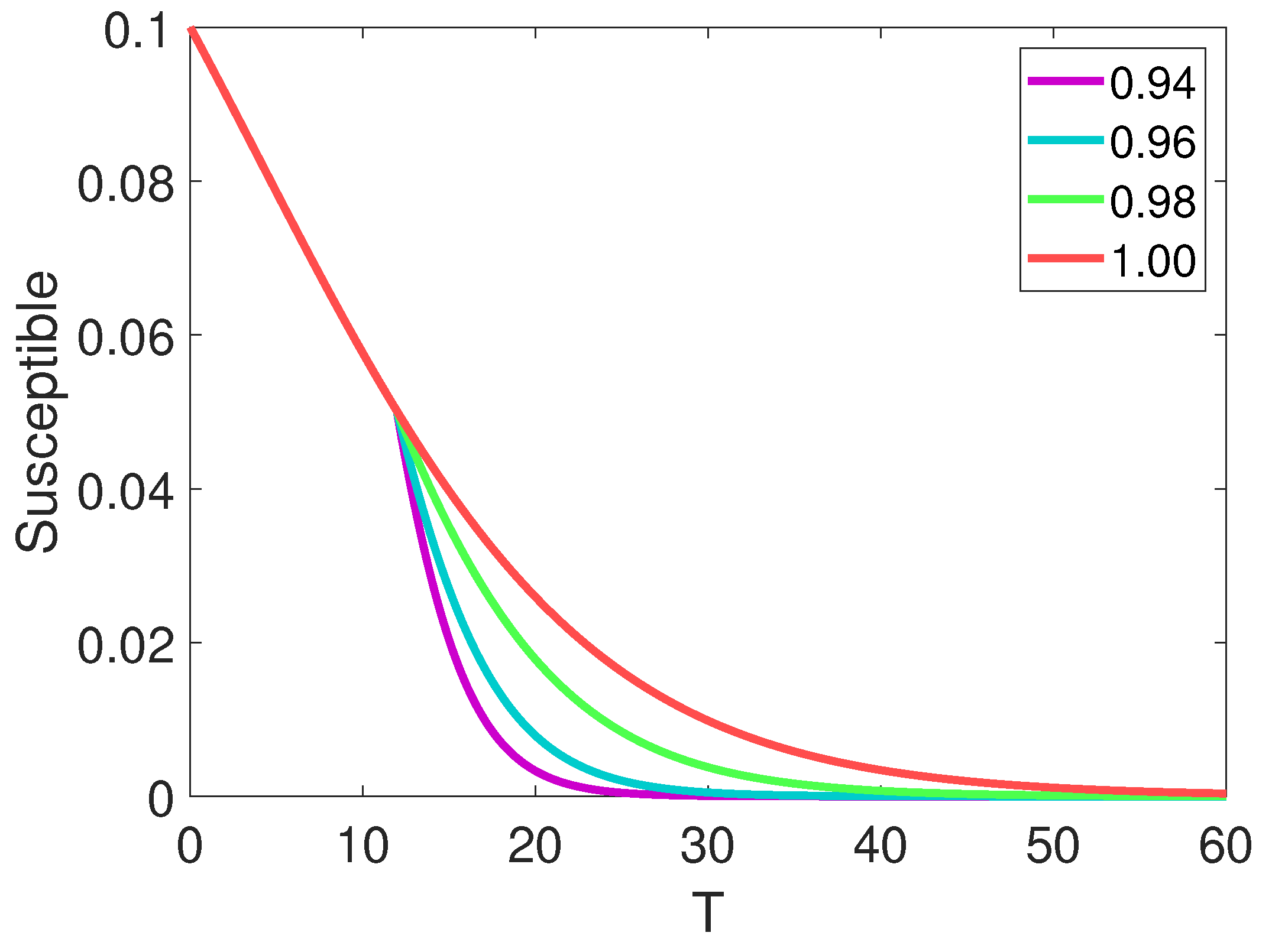
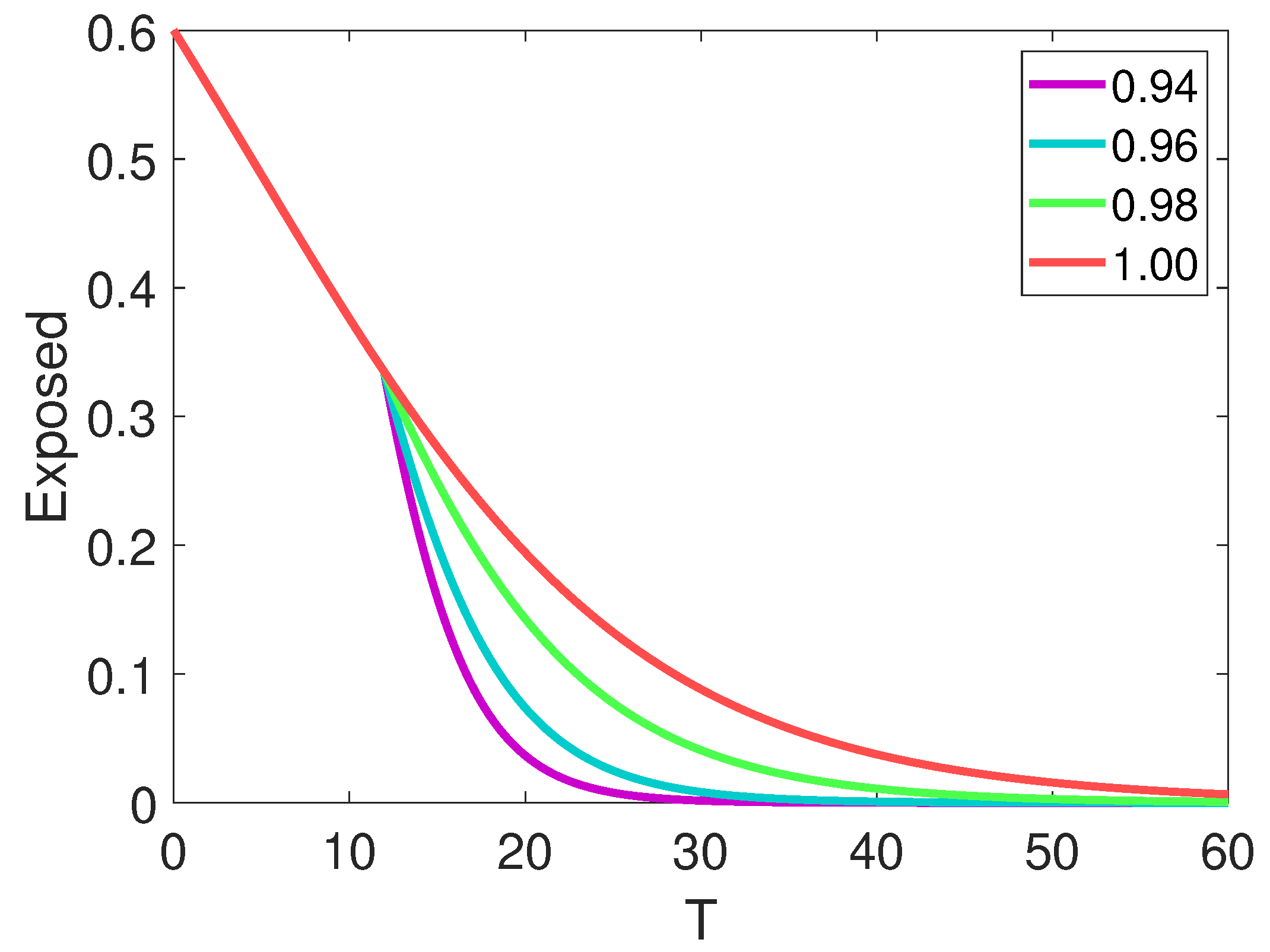
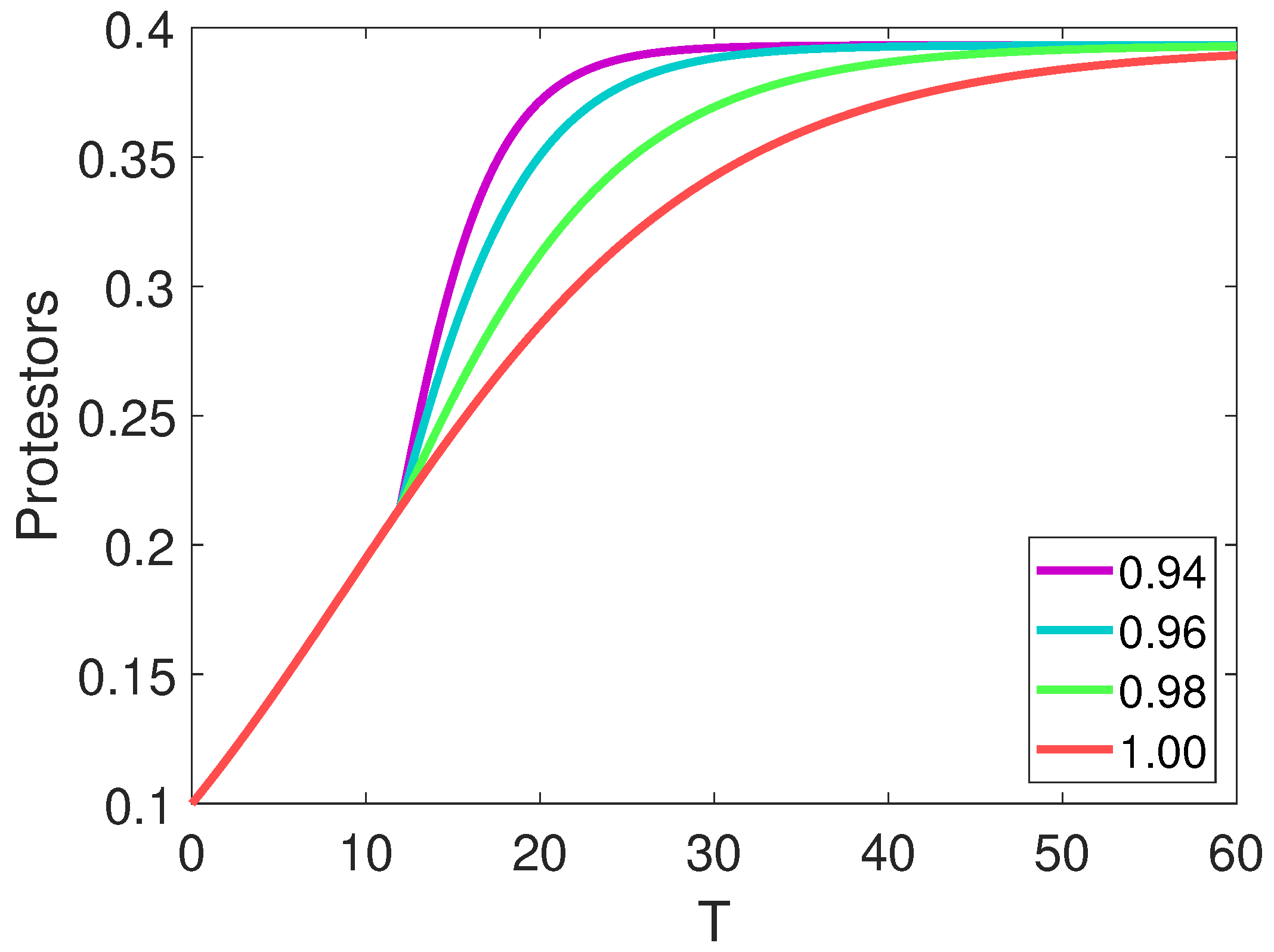
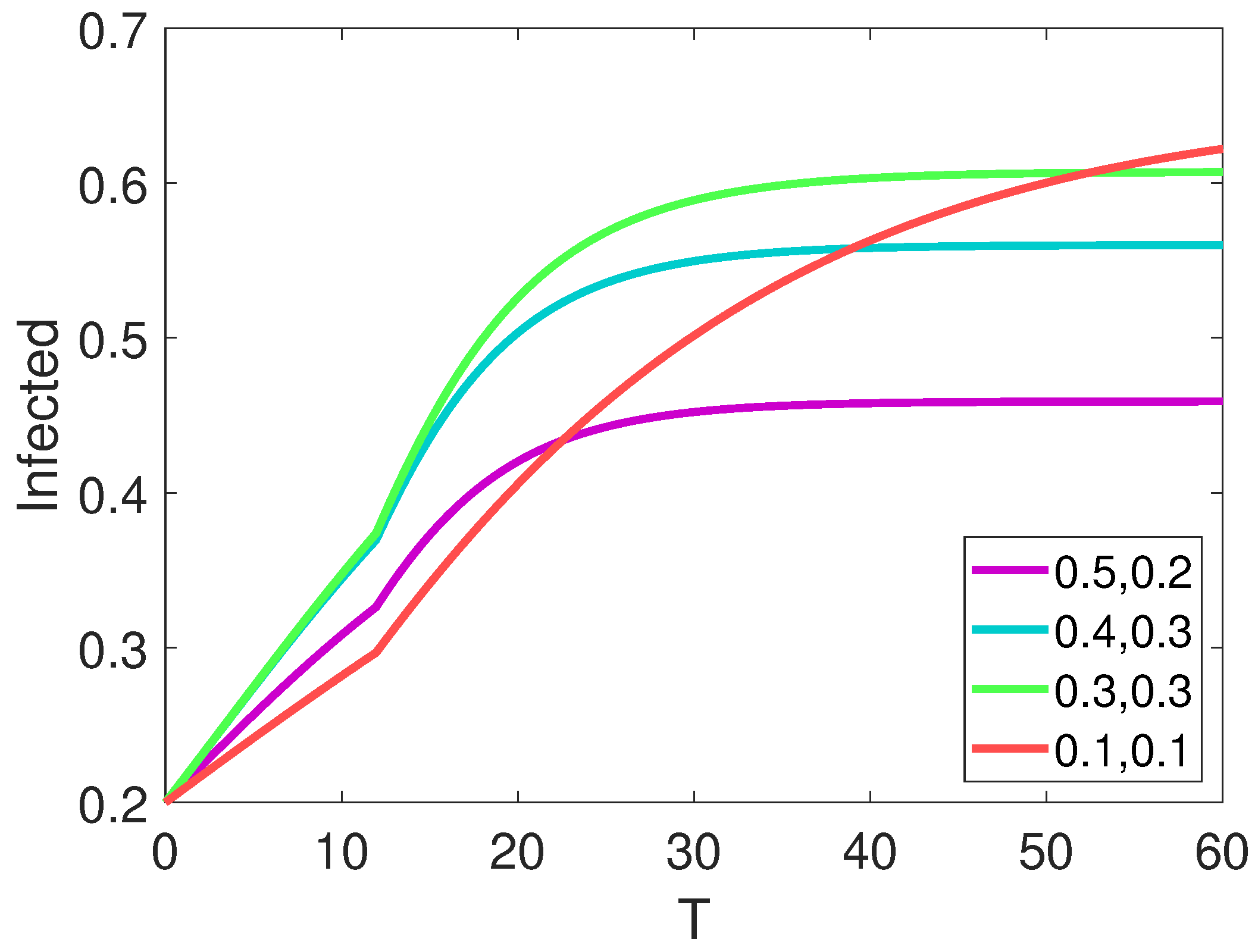
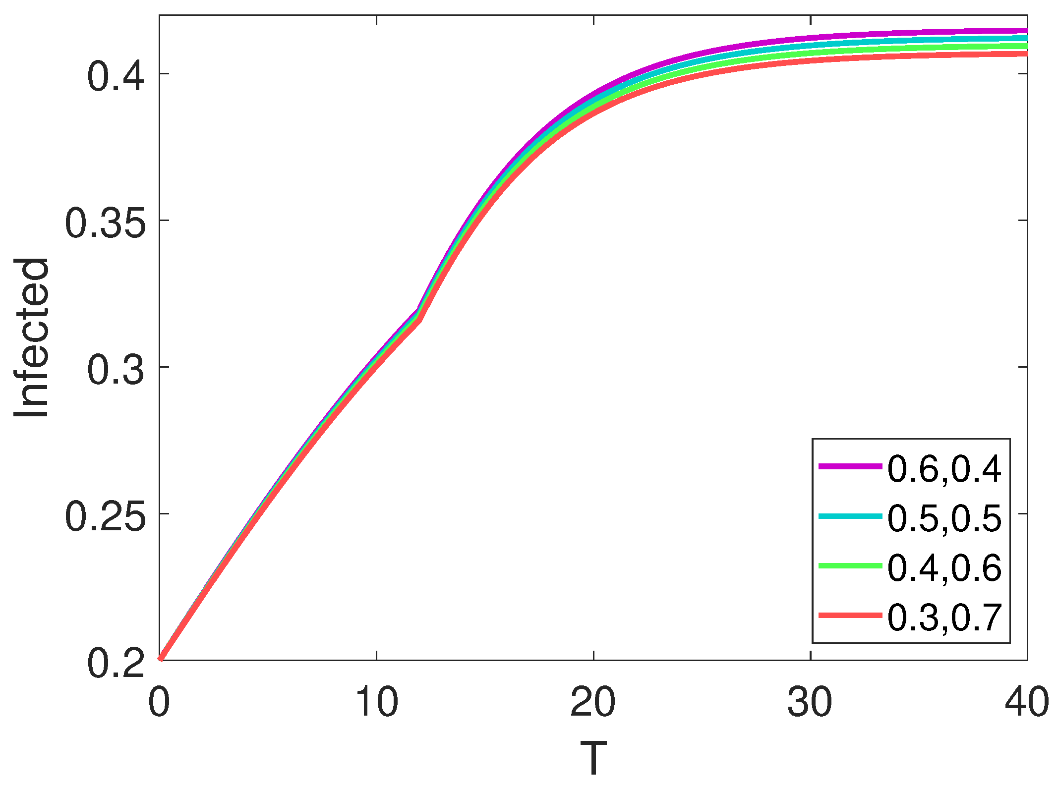
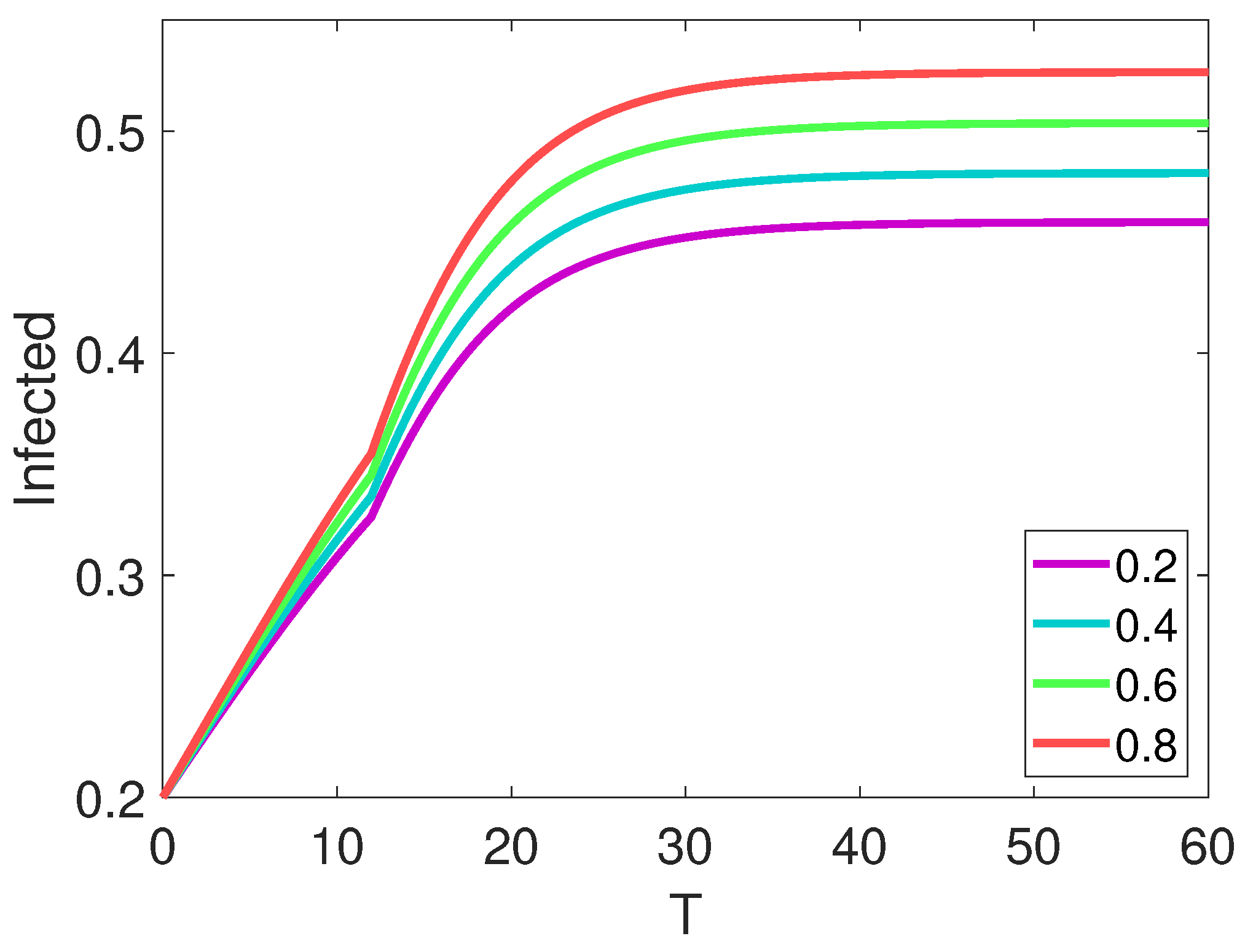
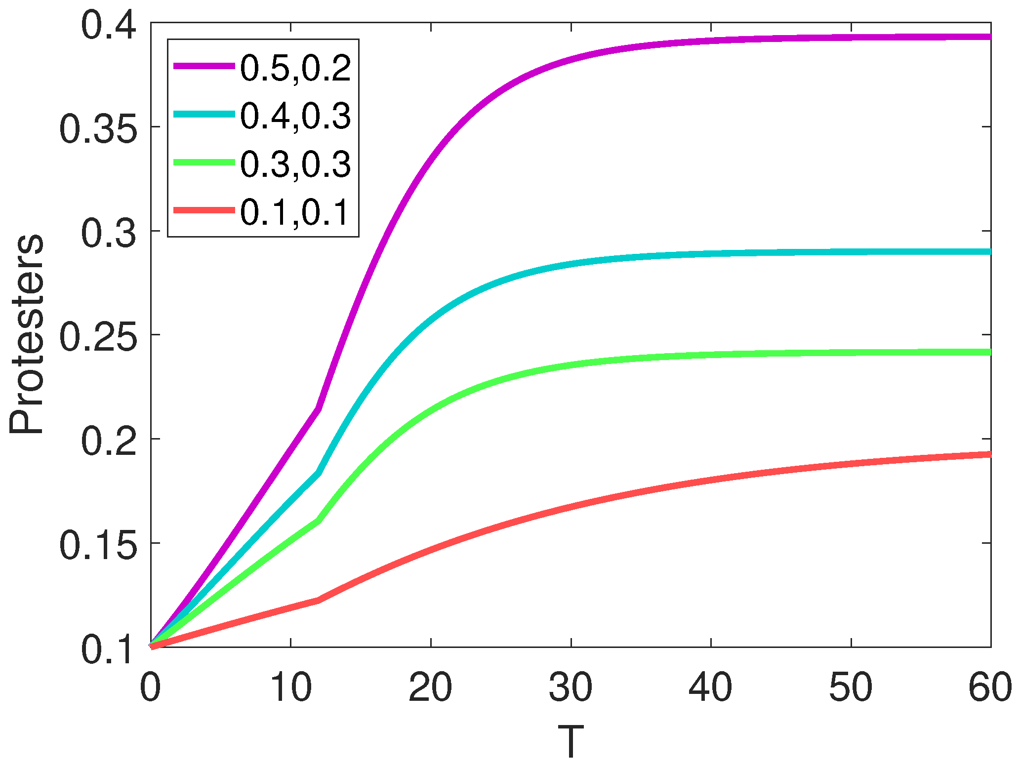
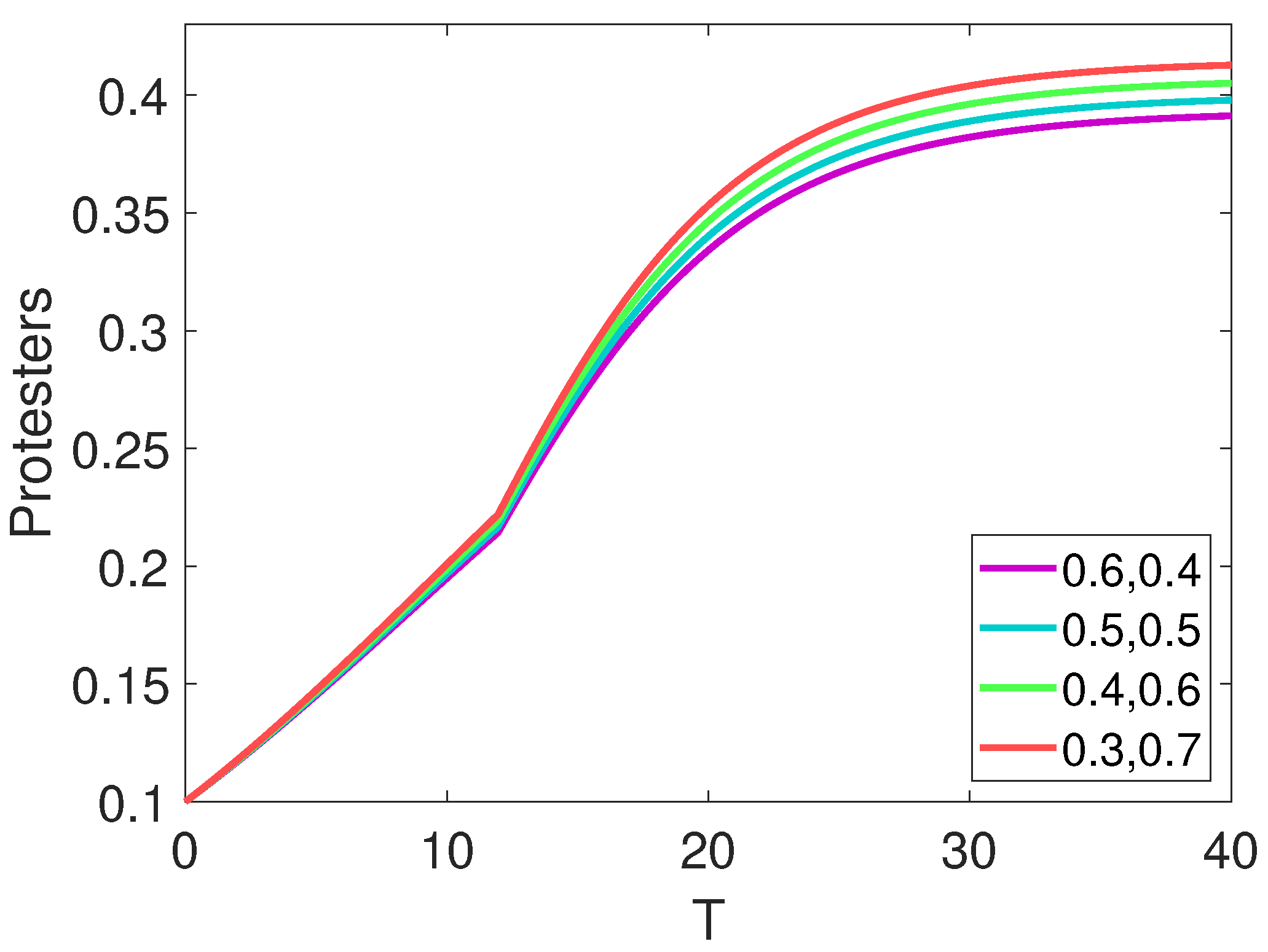
7. Results
8. Concluding Remarks
Author Contributions
Funding
Data Availability Statement
Conflicts of Interest
References
- Allport, G.W.; Postman, L. The Psychology of Rumor; Holt Rinehart and Winston: New York, NY, USA, 1947. [Google Scholar]
- Bordia, P.; Difonzo, N. Psychological motivations in rumor spread. Anal. Commer. Rumors Perspect. Mark. Manag. Rumor Preval. Eff. Control Tactics 2005, 87–101. [Google Scholar]
- Ghazzali, R.; Laaroussi, A.E.A.; Bhih, A.E.L.; Rachik, M. On the control of a reaction-diffusion system: A class of SIR distributed parameter systems. Int. J. Dyn. Control 2019, 7, 1021–1034. [Google Scholar]
- Available online: https://zephoria.com/top-15-valuable-facebook-statistics/ (accessed on 1 April 2020).
- Daley, D.J.; Kendall, D.G. Epidemics and rumors. Nature 1964, 204, 1118. [Google Scholar]
- Maki, D.P.; Thompson, M. Mathematical Models and Applications; Prentice-Hall: Englewood Cliffs, NJ, USA, 1973. [Google Scholar]
- Rapoport, A.; Rebhun, L.I. On the mathematical theory of rumor spread. Bull. Math. Biophys. 1952, 14, 375–383. [Google Scholar]
- Zheng, M.H.; Lv, L.Y.; Zhao, M. Spreading in online social networks: The role of social reinforcement. Phys. Rev. E 2013, 88, 012818. [Google Scholar]
- Fan, L.; Wu, W.; Zhai, X.; Xing, K.; Lee, W.; Du, D.-Z. Maximizing rumor containment in social networks with constrained time. Soc. Netw. Anal. Min. 2014, 4, 1. [Google Scholar]
- Jain, A.; Borkar, V.; Garg, D. Fast rumor source identification via random walks. Soc. Netw. Anal. Min. 2016, 6, 62. [Google Scholar]
- Santhoshkumar, S.; Babu, L.D.D. Earlier detection of rumors in online social networks using certainty-factorbased convolutional neural networks. Soc. Netw. Anal. Min. 2020, 10, 20. [Google Scholar]
- Ndii, M.Z.; Carnia, E.; Supriatna, A.K. Mathematical models for the spread of rumors: A review. In Proceedings of the 6th International Congress on Interdisciplinary Behavior and Social Sciences (ICIBSoS 2017), Bali, Indonesia, 22–23 July 2018. [Google Scholar]
- Goffman, W.; Newil, V.A.I. Generalization of epidemic theory: An application to the transmission of ideas. Nature 1964, 204, 225–228. [Google Scholar]
- Zhao, L.; Cui, H.; Qiu, X.; Wang, X.; Wang, J. SIR rumor spreading model in the new media age. Phys. Stat. Appl. 2013, 392, 995–1003. [Google Scholar]
- Ghazzali, R.; Bhih, A.E.; Laaroussi, A.E.A.; Rachik, M. Modeling a Rumor Propagation in Online Social Network: An Optimal Control Approach. Discret. Dyn. Nat. Soc. 2020, 2020, 6724815. [Google Scholar]
- Singh, J. A new analysis for fractional rumor spreading dynamical model in a social network with Mittag-Leffler law. Chaos: Interdiscip. J. Nonlinear Sci. 2019, 29, 013137. [Google Scholar]
- Ren, G.; Yu, Y.; Lu, Z.; Chen, W. A Fractional Order Model for Rumor Spreading in Mobile Social Networks from A Stochastic Process. In Proceedings of the 2021 9th International Conference on Systems and Control (ICSC), Caen, France, 24–26 November 2021; pp. 312–318. [Google Scholar]
- Li, B.; Liang, H.; He, Q. Multiple and generic bifurcation analysis of a discrete Hindmarsh-Rose model. Chaos Solitons Fractals 2021, 146, 10856. [Google Scholar]
- Li, B.; Eskari, Z.; Avazzadeh, Z. Dynamical behaviors of an SIR epidemic model with discrete time. Fractal Fract. 2022, 6, 659. [Google Scholar]
- Li, B.; Liang, H.; Shi, L.; He, Q. Complex dynamics of Kopel model with nonsymmetric response between oligopolists. Chaos Solitons Fractals 2022, 156, 111860. [Google Scholar]
- Eskari, Z.; Avazzadeh, Z.; Ghaziani, R.K.; Li, B. Dynamics and bifurcations of a discrete-time Lotka—Volterra model using nonstandard finite difference discretization method. Math. Methods Appl. Sci. 2022. [Google Scholar] [CrossRef]
- He, Q.; Zhang, X.; Xia, P.; Zhao, C.; Li, S. A Comparison Research on Dynamic Characteristics of Chinese and American Energy Prices. J. Glob. Inf. Manag. (JGIM) 2023, 31, 1–16. [Google Scholar]
- Zhang, X.; Ding, Z.; Hang, J.; He, Q. How do stock price indices absorb the COVID-19 pandemic shocks? N. Am. J. Econ. Financ. 2022, 60, 101672. [Google Scholar]
- Zhang, X.; Yang, X.; He, Q. Multi-scale systemic risk and spillover networks of commodity markets in the bullish and bearish regimes. N. Am. J. Econ. Financ. 2022, 62, 101766. [Google Scholar]
- Atangana, A.; Baleanu, D. New fractional derivatives with non-local and non-singular kernel. Theory Appl. Heat Transf. Model. Therm. Sci. 2016, 20, 763–769. [Google Scholar]
- Zhang, L.; ur Rahman, M.; Arfan, M.; Ali, A. Investigation of mathematical model of transmission co-infection TB in HIV community with a non-singular kernel. Results Phys. 2021, 28, 104559. [Google Scholar]
- Mahmood, T.; Al-Duais, F.S.; Sun, M. Dynamics of Middle East Respiratory Syndrome Coronavirus (MERS-CoV) involving fractional derivative with Mittag-Leffler kernel. Phys. Stat. Mech. Appl. 2022, 606, 128144. [Google Scholar]
- Li, B.; Zhang, T.; Zhang, C. Investigation of financial bubble mathematical model under fractal-fractional Caputo derivative. Fractals 2023, 31, 2350050. [Google Scholar]
- Liu, X.; Arfan, M.; Ur Rahman, M.; Fatima, B. Analysis of SIQR type mathematical model under Atangana-Baleanu fractional differential operator. Comput. Methods Biomech. Biomed. Eng. 2023, 26, 98–112. [Google Scholar]
- Liu, X.; ur Rahmamn, M.; Ahmad, S.; Baleanu, D. A new fractional infectious disease model under the non-singular Mittag–Leffler derivative. Waves Random Complex Media 2022, 1–27. [Google Scholar] [CrossRef]
- Atangana, A.; Araz, S.İ. New concept in calculus: Piecewise differential and integral operators. Chaos Solitons Fractals 2021, 145, 110638. [Google Scholar]
- Hassan, T.; Khan, J.; Saifullah, S.; Zaman, G. A novel mathematical model of smoking: An integer and piece-wise fractional approach. Eur. Phys. J. Plus 2022, 137, 1219. [Google Scholar]
- Ur Rahman, M.; Arfan, M.; Baleanu, D. Piecewise fractional analysis of the migration effect in plant-pathogen-herbivore interactions. Bull. Biomath. 2023, 1, 1–23. [Google Scholar]
- Qu, H.; Saifullah, S.; Khan, J.; Khan, A.; Ur Rahman, M.; Zheng, G. Dynamics of leptospirosis disease in context of piecewise classical-global and classical-fractional operators. Fractals 2022, 30, 2240216. [Google Scholar]
- El-Shorbagy, M.A.; ur Rahman, M.; Alyami, M.A. On the analysis of the fractional model of COVID-19 under the piecewise global operators. Math. Biosci. Eng. 2023, 20, 6134–6173. [Google Scholar]


| Variables | Description |
|---|---|
| Contact rate from to | |
| b | Contact from to |
| Contact from to | |
| Incubation rate | |
| Contact rate from to | |
| Transmission rate from to | |
| Transmission rate from to | |
| Transmission rate from to through contact with | |
| Infection rate from to through contact with | |
| Probability rate through contact with protesters | |
| Probability rate through contact with protesters | |
| Probability rate through contact with infected | |
| Probability rate through contact with infected |
| Parameters | Values | Parameters | Values |
|---|---|---|---|
| 0.1 | 0.4 | ||
| 0.1 | 0.1 | ||
| 0.5 | 0.4 | ||
| 0.03 |
Disclaimer/Publisher’s Note: The statements, opinions and data contained in all publications are solely those of the individual author(s) and contributor(s) and not of MDPI and/or the editor(s). MDPI and/or the editor(s) disclaim responsibility for any injury to people or property resulting from any ideas, methods, instructions or products referred to in the content. |
© 2023 by the authors. Licensee MDPI, Basel, Switzerland. This article is an open access article distributed under the terms and conditions of the Creative Commons Attribution (CC BY) license (https://creativecommons.org/licenses/by/4.0/).
Share and Cite
Alkahtani, B.S.T.; Alzaid, S.S. Studying the Dynamics of the Rumor Spread Model with Fractional Piecewise Derivative. Symmetry 2023, 15, 1537. https://doi.org/10.3390/sym15081537
Alkahtani BST, Alzaid SS. Studying the Dynamics of the Rumor Spread Model with Fractional Piecewise Derivative. Symmetry. 2023; 15(8):1537. https://doi.org/10.3390/sym15081537
Chicago/Turabian StyleAlkahtani, Badr Saad T., and Sara Salem Alzaid. 2023. "Studying the Dynamics of the Rumor Spread Model with Fractional Piecewise Derivative" Symmetry 15, no. 8: 1537. https://doi.org/10.3390/sym15081537
APA StyleAlkahtani, B. S. T., & Alzaid, S. S. (2023). Studying the Dynamics of the Rumor Spread Model with Fractional Piecewise Derivative. Symmetry, 15(8), 1537. https://doi.org/10.3390/sym15081537