1. Introduction
Iterative methods play a crucial role in solving complex nonlinear equations of the form
where
represents a real function defined on an open interval
D. With diverse applications spanning scientific and engineering domains, the computation of nonlinear Equation (
1) remains a common yet formidable challenge due to the lack of analytical methods. However, iterative methods provide approximate solutions to nonlinear Equation (
1) with high accuracy.
Let
be a simple root of (
1) and
be an initial approximation to
. Then,
and
. The most widely used iterative method for finding the simple root of (
1) is given below.
which is the well-known Newton method [
1]. It is a one-point without-memory method with a quadratic order of convergence.
In the past few decades, various optimal multi-point without-memory methods have been developed for the computation of approximated simple roots [
2,
3,
4,
5,
6]. The concept of an optimal without-memory method is rooted in Kung–Traub’s conjecture [
7]. This conjecture proposes that a multi-point without-memory iterative method, which requires
q function evaluations per iteration, achieves optimality when its convergence order is precisely
. The Newton method (
2) is optimal for
. However, the evaluation of the derivative in the Newton method is a setback for many problems where derivative evaluation is complicated or even does not exist.
To obtain a derivative-free variant of the Newton method (
2), the first derivative
in (
2) is approximated using the first-order Newton divided difference
where
is any real parameter, Equation (
2) can be expressed as
which corresponds to the Traub–Steffensen method [
1]. By setting
, we obtain the well-known Steffensen method [
8]. To assess the efficiency of an iterative method, Ostrowski [
9] introduced the efficiency index
, where
q represents the number of function evaluations per iteration and
p denotes the order of convergence.
The extension of without-memory methods into with-memory methods using accelerating parameters have gained much attention in recent years [
10,
11,
12,
13]. In multi-point with memory iterative methods, the order of convergence is significantly increased without any additional function evaluation by using information from the current as well as the previous iterations. In this paper, we introduce new derivative-free families of three-parametric three-point and four-parametric four-point with and without-memory methods for finding simple roots of nonlinear equations. The formulation of the methods is based on the derivative-free biparametric families of without-memory methods developed in [
14] and by using accelerating parameters without any additional function evaluations for the with-memory methods. As a result, the orders of convergence of the with-memory methods increase from 4 to 7.5311 and 8 to 15.5156. The accelerating parameters are approximated using Newton’s interpolating polynomials so as to obtain highly efficient with-memory methods.
The subsequent sections of this paper are organised as follows.
Section 2 provides the development of modified derivative-free families of without-memory methods, including an in-depth analysis of their theoretical convergence properties. In
Section 3, we delve into the derivation and convergence analysis of the derivative-free families of with-memory methods. The numerical experiments and comparative study of the proposed with and without-memory methods against existing approaches on various test functions, including real-world problems, are presented in
Section 4 to assess the effectiveness and applicability of our proposed methods. In this section, we also explore the dynamical properties of the methods through the study of basins of attraction, revealing the presence of reflection symmetry in all provided basins of attraction. Finally,
Section 5 concludes this paper with key remarks and observations.
2. Modified Families of Three- and Four-Parametric Without-Memory Methods
In this section, we present the new modified derivative-free families of three- and four-parametric multi-point without-memory methods of optimal order in two separate subsections.
2.1. Modified Families of Three-Parametric Three-Point Without-Memory Methods
First, let us consider the following two derivative-free families of biparametric three-point without-memory methods [
14].
where
and
.
From here, we introduce a new parameter
through the modification of
as follows:
Now, substituting the above Equation (
7) in Equations (
5) and (
6), we get two new three-parametric families of without memory iterative methods. These modified methods, denoted as Modified Methods (MM), are defined as follows:
Modified Method 4a (MM): Modified Method 4b (MM): These modified methods adhere to Kung–Traub’s conjecture, requiring three evaluations of the function at each iteration and exhibit an efficiency index of .
Next, we explore the theoretical convergence analysis of the newly introduced modified methods, specifically MM and MM, as outlined in the following theorem.
Theorem 1. Let an initial approximation be close enough to the root α of a sufficiently differentiable real function , where D is an open interval. Then, the modified methods MM (8) and MM (9) exhibit a fourth order of convergence for any {0}. Additionally, both the methods have the same error equation given bywhere , and is the error at iteration. Proof. The proof of Modified Method 4a (MM):
Let the error at
iteration be
. Then, employing the Taylor’s series expansion in the vicinity of
, we obtain
where
. By using
,
, expanding
using Taylor’s series yields
where
are functions of
, i.e.,
, etc.
Then, using (
11) and (
12), we have
where
are functions of
, i.e.,
etc.
Using (
11), (
12) and (
13), we can write
where
are functions of
.
Then, by employing (
14),
is obtained as follows:
With the help of (
11)–(
15), we obtain
where
are functions of
.
Now, putting the values of Equations (
11)–(
16) into the final step of Modified Method 4a (MM
) (
8), we get the following expression for the error equation:
which confirms the optimal fourth order for the Modified Method 4a (MM
) (
8). Similarly, we can prove the optimal fourth order convergence for the Modified Method 4b (MM
) (
9). The proof of the theorem is completed. □
2.2. Modified Families of Four-Parametric Four-Point Without-Memory Methods
Here, we examine the derivative-free families of biparametric four-point without-memory methods proposed in [
14].
where
and
.
Now, we introduce a new parameter
through the modification of
as follows:
Then, substituting the above Equation (
20) as well as Equation (
7) into Equations (
18) and (
19) yields two new four-parametric families of without-memory iterative methods. These modified methods, denoted as Modified Methods (MM), are defined as follows:
Modified Method 8a (MM): Modified Method 8b (MM): Modified methods MM and MM are optimal as per Kung–Traub’s conjecture, require four function evaluations per iteration, and exhibit an efficiency index of .
Next, we delve into the theoretical convergence analysis of the newly introduced modified methods, namely MM and MM, as outlined in the following theorem.
Theorem 2. Let an initial approximation be close enough to the root α of a sufficiently differentiable real function , where D is an open interval. Then, the modified methods MM (21) and MM (22) exhibit the eighth order of convergence for any {0}. In addition, the methods MM and MM have the same error equation given bywhere , and is the error at iteration. Proof. The proof of Modified Method 8a (MM):
Considering all the assumptions made in Theorems 1, from Equation (
17), we have
where
are functions of
.
Using the above Equation (
24), we have
Applying Equations (
11), (
12), (
15), (
24) and (
25), the approximation of
is obtained as follows:
where
are functions of
.
Now, substituting the values of Equations (
12), (
24)–(
26) in the last step of Equation (
21), we obtain the error equation as follows:
which confirms the optimal eight order for the Modified Method 8a (MM
) (
21). Similarly, we can prove the optimal eighth order convegence for the modified method MM
(
22). This completes the proof of the theorem. □
Remark 1. From Theorems 1 and 2, the analysis of the error Equations (10) and (23) shows that the convergence order of the new modified derivative-free families of without-memory methods (MM MM, MM MM) can be increased significantly without any additional function evaluations using the free parameters γ, β, λ and θ, i.e., by putting , , and . However, the exact values of , , , and are not known to us. So, the parameters γ, β, λ, and θ have to be approximated using known information available from the current as well as the previous iterations. This will be the basis for extending the modified derivative-free families of without-memory methods into derivative-free with-memory methods.
3. New Families of Three- and Four-Parametric With-Memory Methods
In this section, we shall discuss the extension of the new modified derivative-free families of without-memory methods presented in
Section 2 into their respective with=memory versions under two separate subsections. Using the available free parameters as accelerating parameters, we aim to increase the convergence order without any additional function evaluations per iteration thereby obtaining highly efficient multi-point with-memory methods.
Let us now discuss in detail the formulation of the methods, the approximations of the accelerating parameters, and the convergence analysis of the with-memory methods in the following subsections.
3.1. Three-Parametric Three-Point With-Memory Methods
Here, we introduce new derivative-free with-memory methods based on the newly suggested modified fourth order derivative-free families of without-memory methods MM
(
8) and MM
(
9).
From error Equation (
10), the convergence order of the methods MM
(
8), and MM
(
9) can be increased from 4 to 8 without any additional function evaluation if we take
,
and
, where
,
. However, the problem is that the exact values of
,
and
are not available to us. So, we use the approximations
,
and
, where
,
and
are the accelerating parameters computed using the available information from the current as well as the previous iterations such that the following conditions are satisfied:
Now, we consider the following approximations for the accelerating parameters
,
and
.
where
,
and
are the respective Newton’s interpolating polynomials of third, fourth, and fifth degrees passing through the best saved points, i.e.,
Now, applying the approximations of the three accelerating parameters
,
and
from (
28) in the methods MM
(
8) and MM
(
9), we obtain the following new derivative-free with-memory methods.
New With-Memory Method 4a (NWMM): For a given
,
, we have
. Then,
New With-Memory Method 4b (NWMM): For a given
,
, we have
. Then,
In order to prove the convergence order of methods NWMM
(
29) and NWMM
(
30), we first present the following lemma.
Lemma 1. If , and , , then the following estimateshold, where , , , and , , are some asymptotic constants. Proof. The proof is similar to Lemma 1 of [
12]. □
Now, we state and prove the following theorem for obtaining the R-order of convergence [
8] of the new three-point with-memory methods NWMM
(
29) and NWMM
(
30).
Theorem 3. If an initial approximation is sufficiently close to the root α of , the parameters , and are calculated by the expressions (28), then the R-order of convergence of the methods NWMM (29) and NWMM (30) is at least 7.5311. Proof. Let the sequence of approximations
produced by the method NWMM
(
29) converges to the root
with order
r. Then, we can write
where
Assuming the iterative sequences
,
have orders
, respectively, then using (
34) and (
35) gives
Using Theorem 1 and Lemma 1, we get
Now, comparing the corresponding powers of
on the right hand sides of (
37), and (
39), (
38) and (
40), (
36) and (
41), we get
This system of equations has the non-trivial solution
and
. Hence, the R-order of convergence of the method NWMM
(
29) is at least
. The R-order of convergence for the methods NWMM
(
30) can be proved in a similar manner. The proof is complete. □
3.2. Four-Parametric Four-Point With-Memory Methods
Here, we introduce new derivative-free with-memory methods which are extensions of the newly suggested modified eighth order derivative-free families of without-memory methods MM
(
21) and MM
(
22).
It is evident from error Equation (
23) that the convergence order of the methods MM
(
21), and MM
(
22) can be increased from 8 to 16 if we take
,
,
and
, where
,
,
. In a similar manner to the previous subsection, we use the approximations
,
,
, and
, where
,
,
, and
are the accelerating parameters computed using the available information from the current as well as the previous iterations such that the following conditions are satisfied:
Now, we consider the following approximations for the accelerating parameters
,
,
and
.
where
,
,
, and
are the respective Newton’s interpolating polynomials of fourth, fifth, sixth, and seventh degrees passing through the best saved points, i.e.,
Now, applying the approximations of the four accelerating parameters
,
,
, and
from (
43) in the modified methods MM
(
21) and MM
(
22), we obtain the following new derivative-free with-memory methods.
New With-Memory Method 8a (NWMM): For a given
,
,
, we have
. Then,
New With-Memory Method 8b (NWMM): For a given
,
,
, we have
. Then,
In order to prove the convergence order of methods NWMM
(
44) and NWMM
(
45), we first present the following lemma.
Lemma 2. If , , , and , , then the following estimateshold, where , , , and , , , are some asymptotic constants. Proof. The proof is similar to Lemma 1 of [
12]. □
Now, we state and prove the following theorem for obtaining the R-order of convergence [
8] of the new four-point with-memory methods NWMM
(
44) and NWMM
(
45).
Theorem 4. If an initial approximation is sufficiently close to the root α of , the parameters , , , and are calculated by the expressions (43), then the R-order of convergence of the methods NWMM (44) and NWMM (45) is at least 15.5156. Proof. Let the sequence of approximations
produced by the method NWMM
(
44) converges to the root
with order
r. Then, we can write
where
Assuming the iterative sequences
,
and
have orders
, and
, respectively, then using (
50) and (
51) gives
Using Theorem 2 and Lemma 2, we get
Now, comparing the corresponding powers of
on the right hand sides of (
53) and (
56), (
54) and (
57), (
55) and (
58), (
52) and (
59), we get
This system of equations has the non-trivial solution
,
and
. Hence, the R-order of convergence of the method NWMM
(
44) is at least
. The R-order of convergence for the methods NWMM
can be proved in similar manner. The proof is complete. □
4. Numerical Experiments
In this section, we examine the performance and the computational efficiency of the newly developed with and without-memory methods discussed in
Section 2 and
Section 3 and compare with some methods of similar nature available in the literature. In particular, we have considered for the comparison the following derivative-free three-parametric methods: FZM
(4.1) [
15], VTM
(28) [
16], and SM
(4.1) [
17], and the following four-parametric methods: AJM
[
13], ZM
(ZR1 from [
18]), and ACM
(M1 from [
19]).
All numerical tests have been executed using the multi-precision arithmetic programming software Mathematica 12.2. For all methods, we have chosen the same values of the parameters in all the test functions in order to start the initial iteration. These same values are used for the corresponding parameters of all the compared methods in order to have uniform and fair comparison in all the test functions.
Numerical test functions which comprise a standard academic example and some real-life chemical engineering problems along with their simple roots and initial guesses are presented below.
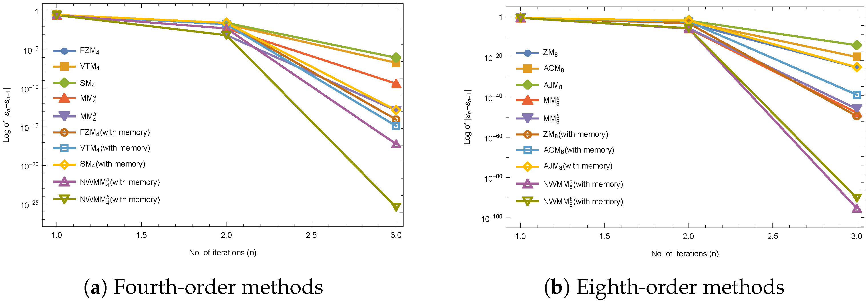
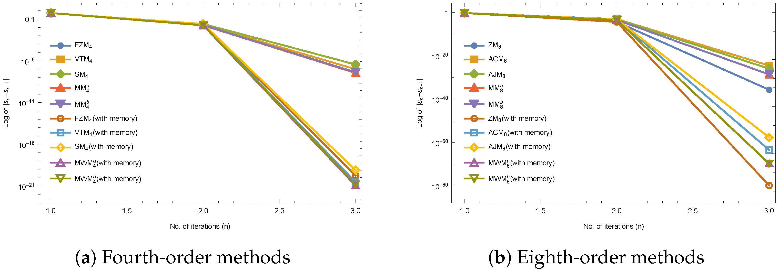
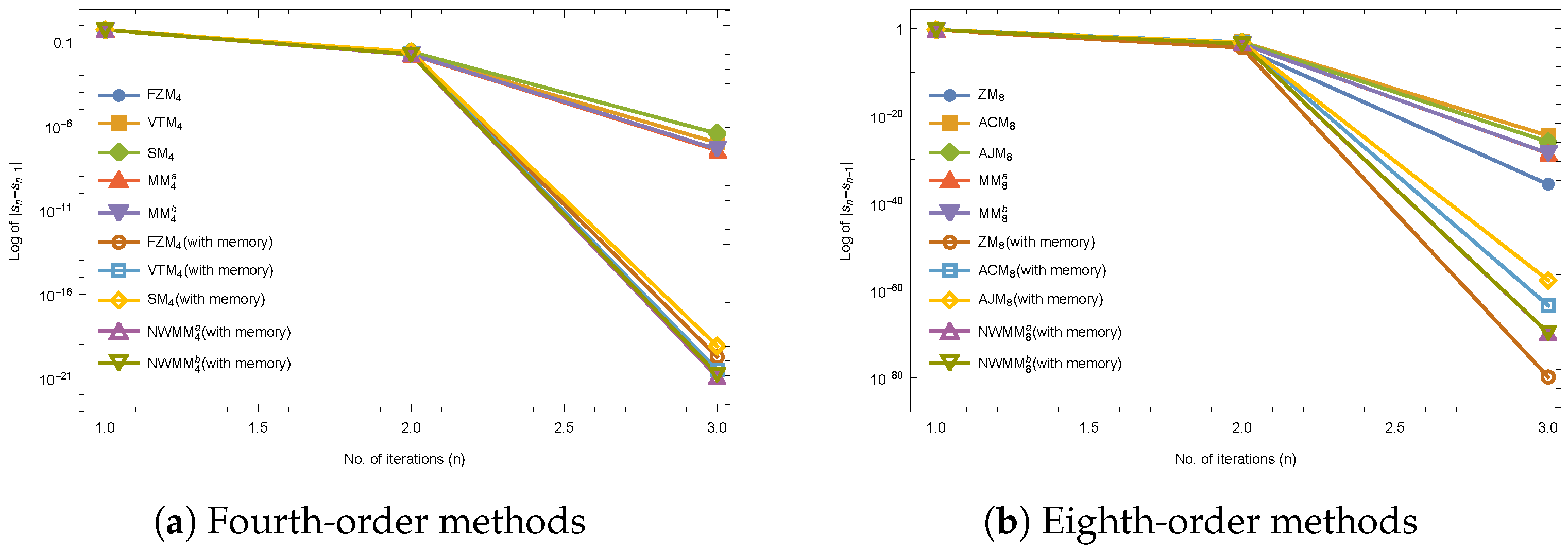
Example 1. A standard academic test function given by It has a simple root . We use as the initial guess and the results are displayed in Table 1. Example 2. The Michaelis–Menten model [20] describes the kinetics of enzyme-mediated reactions and has the following expression:where S is the substrate concentration (moles/L), is the maximum uptake rate (moles/L/d), and is the half-saturation constant, which is the substrate level at which uptake is half of the maximum (moles/L). If is the initial substrate level at , then the above equation can be solved for S as follows: For a particular case where , moles/L, moles/L/d, and moles/L, the above equation reduces to the following nonlinear function.where s denotes the substrate concentration S to be determined. The nonlinear equation has a simple root . We use as the initial guess and the results are displayed in Table 2. Example 3. Let us consider the conversion of the fraction of Nitrogen–Hydrogen feed into Ammonia, called fractional conversion, at a pressure of 250 atm and temperature of (see [21] for details). When reduced to the polynomial form, the problem has the following expression: The nonlinear equation has a simple root . We take as the initial guess and the results are displayed in Table 3. Example 4. The equation of state for a van der Waals fluid takes the following form [22]:where , and R are positive constants, P is the pressure, T is the absolute temperature, and V is the molar volume. Now, let us substitute , and , where is the critical pressure, is the critical temperature, and is the critical molar volume.
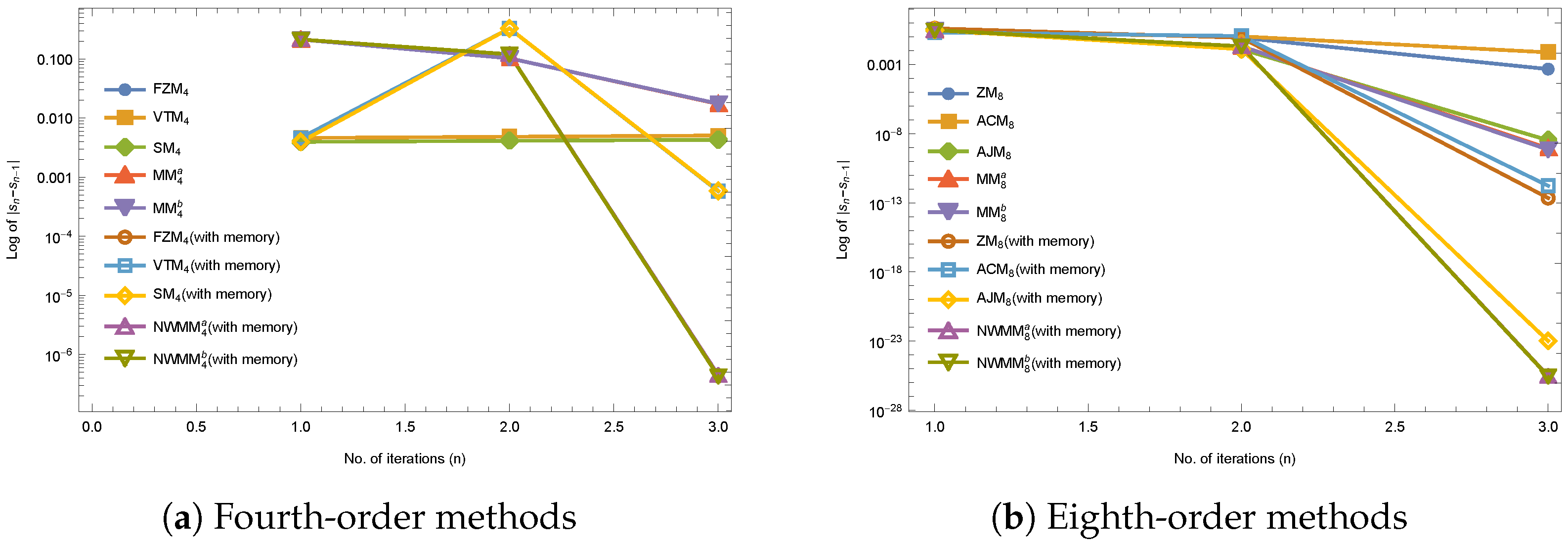
Then, the above Equation (66), in which the pressure, temperature, and volume are expressed in terms of their critical values, becomeswhere , and v are called the reduced pressure, temperature, and volume, respectively. For particular values of and , Equation (67) reduces to the following nonlinear equation.where s represents the reduced volume v to be determined. Equation (68) has a simple root . We use as the initial guess and the results are displayed in Table 4. All the results and analysis of the numerical computations are displayed in
Table 1,
Table 2,
Table 3 and
Table 4. The aim of these tables is to showcase the performance of the iterative methods in terms of their convergence speed and accuracy. We measure the convergence by tracking the number of iterations (
n) required to satisfy the stopping criterion:
where
represents the current iterate and
denotes the absolute residual error of the function. To provide further insights, we also include in the tables the estimated error in consecutive iterations,
, for the initial three iterations. Moreover, we calculate the computational order of convergence (COC) using the formula [
23]:
From
Table 1,
Table 2,
Table 3 and
Table 4, the numerical results reveal the good performance and better efficiency of the proposed with and without-memory methods, thus confirming their theoretical results. The proposed methods show better accuracy with high efficiency in terms of minimal errors after three iterations as compared to the existing methods in comparison.
Table 2,
Table 3 and
Table 4 confirm the applicability of the proposed families of methods when applied to some real world chemical problems. In addition, some of the compared methods fail to converge to the required roots and diverge away from the roots, which is not the case for the proposed families of methods, as can be observed from
Figure 1,
Figure 2,
Figure 3 and
Figure 4. Further, the numerical test results reveal that the COC supports the theoretical convergence order of the new proposed with and without-memory methods in the test functions.
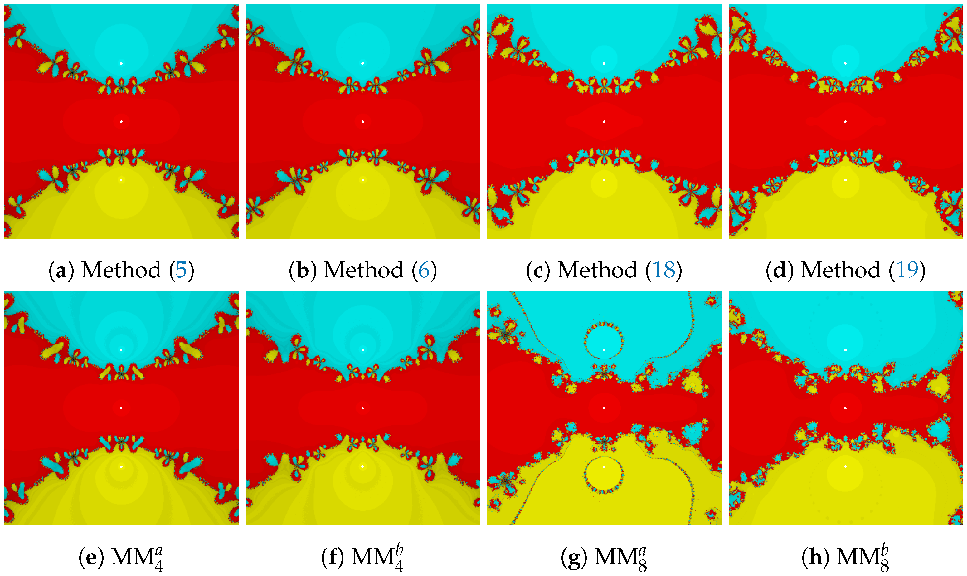
Comparison by Basins of Attraction
In this section, we explore the dynamical properties of the proposed methods discussed in
Section 2. To analyse their behaviour in the complex plane, we examine the basins of attraction associated with each method. Specifically, we compare MM
with Method (
5), MM
with Method (
6), MM
with Method (
18), and MM
with Method (
19), respectively.
We used a
grid to represent the complex plane region
. Each point
in
R was assigned a colour based on the root it converged to using an iterative method. Divergent points were marked in black if they failed to converge within 100 iterations or within a tolerance of
. Simple roots were represented by white circles. Brighter colours indicated faster convergence, while darker colours indicated slower convergence. In
Figure 5, we illustrate the basins of attraction obtained by applying the fourth and eighth-order methods to the function
. To have a fair comparison, we take the same values of the parameters
for all compared methods.
In
Figure 5, it is evident that all the compared methods exhibit large basins of attraction with only a few divergent points. However, the proposed modified methods outperform the biparametric methods due to the inclusion of additional parameters. In fact, the proposed methods MM
and MM
are the best with no divergent points.
Moreover, we can observe from
Table 5 and
Table 6 that each of the proposed methods show significant improvements in terms of fewer divergent points. In particular, MM
shows an improvement of
over method (
5), and
improvement for method MM
over method (
6). Similarly, MM
and MM
show
and
improvements over methods (
18) and (
19), respectively. Notably, both methods MM
and MM
show no divergent points, as observed from
Table 5 and
Table 6, respectively. This underscores the crucial role of the extra parameters in enhancing stability and reducing divergent points in the proposed methods.


