Abstract
The possibility of neutrinos moving at faster-than-light speeds can be modeled using terms in the Lagrangian that violate Lorentz symmetry, but the question of whether and tachyonic neutrinos exist is an empirical question. It remains unresolved despite evidence from cosmic ray and other data that the electron neutrino has an effective which would require that one or more mass states is also tachyonic. In 2013, the model of the neutrino masses, which includes one tachyonic mass state, was proposed based on supernova SN 1987A neutrino data. Here, we update evidence for tachyonic electron neutrinos and the model and discuss one test which could prove conclusive. The update of earlier evidence includes many new elements, including new data which make the earlier cosmic ray evidence more robust, new results on cosmic ray composition, the ankle of the spectrum, leptonic cosmic ray data, and the statistical significance of finding the three large neutrino masses stipulated in the model. Barring a galactic supernova, which occur only around twice a century, a decisive test of the model could involve observing an extragalactic supernova neutrino burst, that is, a cluster of neutrinos in a specific time window well beyond what chance would predict. Even though existing searches for such bursts have yielded only upper limits on the extragalactic supernova frequency within a certain distance, it is shown that the choice of a one-day window for possible neutrino clusters in time might be far more sensitive. A search using a one-day time window could be conducted using existing data, and if a signal is found it would confirm the model. Of course, the absence of any day-long neutrino burst would not disprove the model, since it could mean only that the nearest supernova during the period when detectors were active was simply too far to be detected. Finally, apart from testing the model, an alternative type of search is suggested using existing hadronic cosmic ray data (from the IceCube Collaboration) that might verify the tachyonic neutrino hypothesis.
1. Neutrinos as Tachyons?
This review article updates and strengthens the evidence that some neutrinos are tachyons, i.e., and particles [1] and it suggests several analyses of existing data that could serve as definitive tests of that hypothesis. The idea that some neutrinos might be tachyons can be traced back to a 1972 suggestion by Cawley [2]. However, it was not until Chodos, Hauser and Kostelecky proposed a model for them that the idea was taken seriously [3]. Many searches for evidence that neutrinos are tachyons have been made since then, and all have proven inconclusive [4]. The present paper is a natural extension of that earlier review, one that strengthens the evidence for tachyonic neutrinos, particularly in respect to data from cosmic rays, SN 1987A, and extragalactic supernovae. The evidence for neutrinos being tachyons is inconclusive not negative as long as no neutrinos have been shown to have either or Moreover even if an experiment should find a effective mass for the electron neutrino, and not just an upper limit, the possibility of one of the two other flavors being tachyonic would probably remain indefinitely, given the large best value and upper limit on the muon and tau neutrino masses: and [5].
The effective mass of the muon neutrino is measured in the decay and that of the tau neutrino is measured in the processes and [6]. Barring some completely novel way of measuring the masses of and it is extremely doubtful if the measurement uncertainties in the three decay processes could ever be reduced by enough to yield upper limits comparable to the scale expected for those two neutrino masses, which is why it is only for the electron flavor that matter of a possible tachyonic nature is likely to be empirically resolvable. Comparing and , it is interesting that the measurement of the tau neutrino mass is found by measuring as many as 21 quantities, i.e., the vector momentum of as many as 7 particles, while the mass of the muon neutrino can be made by measuring a single quantity, namely the magnitude of the muon kinetic energy in the decay in which the initial pion can be considered to be at rest. That is one reason for the much larger uncertainty in the mass of compared to
The negative best value of the muon neutrino mass squared cited above is, of course, of no significance, given the size of the uncertainty. For that matter, neither are the negative values found for of the electron neutrino reported in some earlier direct mass experiments, which were certainly due to systematic errors [7] Although many theorists remain highly skeptical about tachyonic neutrinos, some others including Chodos [8], Jentschura [9], Rembieliński and Ciborowski [10], Radzikowski [11], and Schwartz [12] have come up with theories for such particles, and debunked many of the theoretical arguments raised against them. Some of their theories violate Lorentz symmetry and some postulate new symmetries [8] Whatever one’s theoretical arguments for or against the existence of tachyonic neutrinos, ultimately the matter remains one for experiment and/or observations to decide.
2. Cosmic Ray Evidence for
One surprising empirical consequence of tachyonic electron neutrinos was proposed in 1992 by Chodos, Kostelecky, Potting, and Gates [13] based on certain energetically forbidden beta decays (such as a free proton undergoing ) being allowed when the initial proton has an energy above a certain threshold. The idea is that the energy E of an emitted neutrino in the proton rest frame can be expressed in terms of its lab energy, momentum and emission angle as:
Then, since when it follows that E can become more negative than the decay Q-value when is high enough, making the decay energetically allowed for a range of neutrino emission angles, The same argument would apply to the energetically forbidden (negative Q-value) alpha decay, i.e., Although Chodos et al. [13] described possible accelerator experiments, the cosmic rays provide a better test because their energies can far exceed those of existing accelerators. At high energies, the cosmic rays are primarily protons, with a small admixture of alpha particles and heavier nuclei.
2.1. Explaining the Knees
The spectrum of cosmic rays approximately follows a pure inverse cubic power law, which yields a straight line on a log–log plot. As we have noted, if electron neutrinos are tachyons, this would allow an energetically forbidden beta decay of protons or alpha particles to occur above certain threshold energies. In fact, such decays would occur in increasing numbers above their threshold, as the range of allowed decay angles increases. Thus, if the initial spectrum of cosmic rays at their source is a pure power law, we would then find an abrupt increase in the spectral index at the threshold energy for each decay process. Given this consequence of , Ehrlich [14] showed in 1999 that many features of the cosmic ray spectrum could be explained provided the electron neutrino was a tachyon of mass: or .
Suppose the energies of the first and second knees of the spectrum (energies K1 and K2 in Figure 1) represent the onset of proton decay and alpha decay, respectively, for a tachyonic electron neutrino of mass The expected threshold energies for these two decays can be found in terms of the (negative) Q-values, and the relevant masses to be [14]:
and these are just the energies labelled K1 and K2 where the two knees are observed when —see Figure 1. Data from other experiments yield slightly different values for the energies of the knees (not in perfect agreement with the predicted values), but the spectrum in Figure 1 is a particularly clean one, especially in terms of the abruptness of K1, K2, and A.
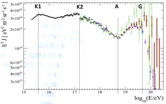
Figure 1.
Plot of the cosmic ray spectrum flux times from Figure 26 of Abassi et al. [15]. Multiplying the flux by makes departures from an power law much more visible. The data shown in four different colors are from four experiments and the Auger data have been rescaled by in energy for better agreement with the other experiments. Lines identifying the energies of four features of the spectrum have been added by the author: K1 = first knee, K2 = second knee, A = ankle, and G = predicted GZK cutoff at Figure used with permission of Tareq AbuZayyad, coauthor of ref. [15].
2.2. Explaining the Ankle
The existence and location of the ankle of the spectrum at energy A also has a natural explanation in terms of the tachyonic neutrino hypothesis. Normally, if protons could decay, one would not expect neutrons from their decay to reach Earth from distant sources, given their short (10 min) lifetime. However, in the tachyon neutrino hypothesis, one has a decay chain: with perhaps 1000 steps [14,16]. At the energy of the ankle the neutron lifetime is extended by a factor of so neutrons and protons could just begin to reach Earth from portions of the local (Virgo) cluster of galaxies (length 100 Mly). This would lead to a rise in the number of undecayed protons reaching Earth from sources located in the local cluster, and hence an upturn in the spectrum (times ) after the ankle. Since our galaxy is at the lower end of the local galaxy cluster which roughly has a linear shape (see Figure 2), the number of sources creating cosmic ray protons that survive the journey to Earth will increase in direct proportion to the energy, and that increase would explain the spectrum shape after the ankle up to the end of the spectrum—see Appendix A for more details. The last of the four features in the spectrum labelled G in Figure 1 is the GZK cut-off [17,18], which is the theoretical highest energy at which cosmic ray protons could reach Earth without being blocked by interaction with the cosmic background radiation photons. The blue data points with small error bars give a much better indication of the true cut-off energy than the black data points with very large error bars.
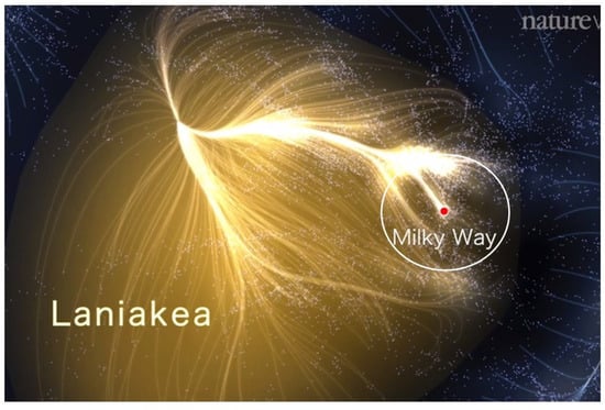
Figure 2.
Supercluster of over 100,000 galaxies known as Laniakea, with the location of the Milky Way Galaxy shown as a dot at the center of the circle is at the lower end of our “local” (Virgo) cluster shown as a line at “11 O’clock” in the diagram. Laniakea stretches 500 Mly across, and the circle (added by author) shows the maximum distance that the highest-energy cosmic rays (160 Mly) could travel to reach Earth based on the GZK cut-off. Given the scale of this map, the Milky Way Galaxy with its several hundred billion stars is about 4000 times smaller than the circle and much tinier than the dot at its center. This image used courtesy of R. Brent Tully, and his coauthors Hélène Courtois, Yehuda Hoffman, and Daniel Pomarède of ref. [19].
2.3. Composition of the Cosmic Rays
If the first knee really is due to proton decay, which is allowed above that energy if , then one would expect that (a) the spectrum just below the knee should be primarily protons, and (b) the proton fraction should be increasingly depleted for energies just above the knee. This predicted variation of the fraction of protons in the cosmic rays is exactly what is found. Thus, according to Figure 7 of ref. [20], just below the knee the spectrum is consistent with being protons and less than a decade above the knee the fraction has declined to ≈10%. Likewise, if the second knee is due to decay, then one should find a similar drop in the contribution across the second knee. According to Figure 6 in ref. [21] recent IceCube data shows that the contribution to be of the total before the second knee and it drops to near zero above the knee, which would agree with the (tachyonic neutrino) interpretation of the second knee as being due to alpha decay.
The ankle of the spectrum, unlike the knees, could not be due to a particle decay, because it is an upturn not a downturn, thus suggesting a gain of some species of particle to the total spectrum. In our earlier explanation of the ankle we noted that because of time dilation, protons could reach us undecayed from more distant sources, the higher the energy becomes, up to the very end of the spectrum. Therefore, under this hypothesis, the fraction of cosmic rays that are protons should steadily rise above the ankle. Data from the Pierre Auger collaboration show the spectrum consists of a mixture of many nuclei at the ankle, including only about protons [22]. We can infer that the proton fraction is rising above the ankle because the spectrum drops off precipitously right at the predicted GZK cut-off shown at or This fact implies the cosmic rays at this energy are nearly protons. Had the cosmic rays instead consisted of nuclei with a atomic number Z, the predicted cut-off energy would be Z times higher. Even a minimal increase from Z = 1 to Z = 2 (He nuclei) would yield a predicted cutoff energy twice as high, i.e., which is grossly inconsistent with the observed cut-off. We conclude from the variation of the proton component with energy above the ankle that the data support the idea that protons are being added to the spectrum from more distant sources as the energy rises above the ankle, as would be expected in our neutrino model. One further important piece of support for our interpretation of the ankle is the expected change in spectral index occurring there, which is described in Appendix A. This result is shown to follow from the linear shape of the Virgo galaxy cluster shown in Figure 2.
In summary, the observed energy of each spectral feature (two knees, ankle, and GZK cut-off) all can be interpreted as supporting a tachyonic electron neutrino of mass . Similarly, the observed changes in spectral composition above and below each of these features also supports that hypothesis.
2.4. IceCube Data and Neutrons?
If an electron neutrino gives rise to proton decay for energies above the knee there should be some evidence of neutrons from those decays in the cosmic rays. Neutrons being unaffected by galactic magnetic fields can reveal their presence because they would mostly point back to their sources. The result would be small regions (“hot spots”) in an otherwise isotropic distribution. Cold spots are another type of small-scale anisotropy, but they would not arise from such cosmic ray neutrons. Given the hypothesized neutron–proton decay chain, hot spots would be largely confined to an energy region just above the first knee. Small-scale regions of excess flux for cosmic rays just above the first knee have in fact been reported, [23] most prominently in IceCube, a very high statistics experiment (577 billion cosmic ray events) [24]. Unlike large-scale anisotropies, those having a small angular scale are surprising and very difficult to account for in any cosmic ray models [25], but they are as noted a natural consequence of the decay
In ref. [24] the IceCube Collaboration shows maps of small-scale anisotropies for a series of nine energy intervals or bins from 10 TeV to In all but one of the energy bins there are few small-scale regions showing hot spots of a magnitude as large as In contrast, the only energy bin just above the knee, i.e., , shows a significant number of such regions, more than any other energy band—see the dark red regions in Figure 3 (bottom map). Importantly, we note that for cold spots there is not any major difference between the energy bin just above the knee and that just below it. Under the conventional explanation of the first knee (being the transition from galactic to extragalactic cosmic rays), one might expect still higher energy bands would show similarly high levels of small scale anisotropy—both hot and cold spots. On the other hand, for the tachyonic neutrino hypothesis, with its“pile-up” of neutrons just above the knee, the hot spots would be limited to that energy region. In fact, earlier data from other limited statistics experiments support this latter possibility [16,23]. Even though IceCube has no data with energies higher than the energy bin, one might be able to use the archived IceCube data, with over half a trillion events, to see if the presence of hot spots is (or is not) confined to the region just above the knee. To test this possibility, one could examine the energy distribution of all the cosmic rays in Figure 3 which are in the dark red (and dark blue) regions, i.e., regions having . If the energy distribution for the hot spots showed a significant peak just above the knee (at ) and that for the cold spots did not, such an outcome would lend significant credibility to the neutron “pile-up” hypothesis, which is a direct consequence of
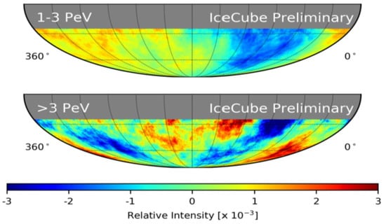
Figure 3.
Small-scale anisotropies observed by the IceCube Collaboration for cosmic rays having an energy range just below the knee (top map) and just above the knee (bottom map). The largest anisotropies observed are at a level of and they are shown in dark red (+) and dark blue (−). Both maps are in equatorial coordinates. Figure is used courtesy of the IceCube Collaboration.
2.5. Leptonic Cosmic Rays: e and
We have seen that many features of the hadronic cosmic ray spectrum have shown consistency with a tachyonic electron neutrino, so one might wonder whether leptonic cosmic rays might confirm or refute this possibility. Consider, for example, the energetically forbidden decay of electrons, i.e., whose predicted threshold would be which would lead to a knee in the spectrum there. As of 2023, measurements of the cosmic ray combined electron and positron spectrum have been made using space and ground-based detectors only up to the 10 TeV energy range. Observing the spectrum shape above 100 TeV might be possible in the future, but it would require improvements in background discrimination beyond those currently envisioned [26].
The spectrum of cosmic ray neutrinos also in principle might provide evidence for the electron neutrino being tachyonic. In Equation (6) of ref. [27] the threshold for the energetically forbidden process is found to be Regrettably, this energy is at the lower end of the sensitivity range of the IceCube experiment, so it is not possible at present to say anything from IceCube (or other currently available) data whether cosmic ray neutrino spectra in fact show the predicted knee at Thus, leptonic cosmic rays neither support not contradict the possibility of a tachyonic electron neutrino.
3. Wanted: A New Neutrino Model
The three flavor state masses for the electron, muon, and tau neutrinos are usually referred to as “effective masses”, because each can be expressed in terms of the three mass state masses according to for In the conventional view, it is assumed based on oscillation data that the three mass state masses are separated by at most in either the normal or inverted hierarchies, that is by about It is important to recall the original basis of this rarely questioned assumption, which is that (a) no third oscillations are observed besides those corresponding to the atmospheric and solar mass differences ( and ) and (b) oscillations having are empirically indistinguishable from those with While the latter is certainly true, the former is not, based on short baseline (SBL) experiments that suggest a third wavelength corresponding to Furthermore, attempts to reconcile these SBL oscillations within the conventional mass hierarchies by adding one or more sterile neutrinos have not been successful, given a tension between appearance and disappearance data, which may call for beyond-standard-model physics, or perhaps instead abandoning the model in which the three active neutrino masses are nearly degenerate.
3.1. The Tachyonic Neutrino Model
The model was published by the author [28] in 2013. The model stipulated three active–sterile neutrino pairs having specific masses, with one pair being tachyons, i.e., The model was inconsistent with the conventional mass hierarchies of the neutrino masses, in which it is assumed that the three active masses are separated by at most . Specifically, the model suggests much more widely separated and larger values for the three masses—see numerical values for and in Figure 4.
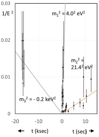
Figure 4.
Plot of versus arrival times t for 30 neutrinos recorded in four detectors on the date of SN 1987A. Note the use of ksec for the five Mont Blanc neutrinos arriving at times prior to the bursts seen in the other three detectors. For clarity, the arrival times for those five neutrinos are shown slightly displaced from each other even though they are all in a 5 s interval. Note that all 30 neutrinos cluster about one (and only one) of the three straight lines shown, and most fall no more than one standard deviation from that line. In the model, each of the three masses is that of an active–sterile doublet having the same fractional mass splitting,
In order to be consistent with the values seen in oscillation experiments, the mass splittings of the three active–sterile doublets are given by and The model further stipulates a constant fractional splitting, i.e., for In ref. [29], ways have been suggested so that the large masses in the model need not be in conflict with either cosmological upper limits on or with upper limits on the electron neutrino mass from the KATRIN experiment. In fact, previously released KATRIN data have been found to fit the model slightly better than the conventional single effective electron neutrino mass [30].
3.2. Origin of Model from SN 1987A Data
The model arose from a striking regularity observed in the SN 1987A neutrino data. Normally, it is assumed that the data can only be used to set an upper limit on the neutrino masses, not actual values. However if the supernova neutrino emissions are nearly simultaneous (to within 1 to 2 s), as Vissani and Rosso [31] have suggested, then from the spread in neutrino travel times and their energies we can compute the masses of neutrinos. Here, T is the light travel time from the supernova, t is the neutrino arrival time relative to a photon, and would apply to tachyonic neutrinos. To see how masses are computed for individual neutrinos, note that in a plot of versus neutrinos of a given mass will be found to lie on straight lines through the origin of slope [32].
In Figure 4 we see the plot for 30 neutrinos (actually mostly antineutrinos) observed on the day of SN 1987A in four detectors. In addition to those seen in Kamiokande, IMB, and Baksan, we have also included the five neutrino events in the Mont Blanc detector, which are normally ignored. The Mont Blanc burst is usually ignored not just because of their 4.8 h early arrival within a 5 s time window, but mainly because no such early burst was detected in the other three detectors. However, this absence can be explained in terms of the very low energies of the five Mont Blanc neutrinos, and the much lower energy threshold of that detector compared to the other three. Thus, the average visible energy was for the 5 Mont Blanc neutrinos, yielding neutrino energies averaging At this low energy, the Kamiokande II detector, the largest of the four, had a detection efficiency of only around 20% [33]. In addition the four detectors were not precisely synchronized, and small bursts in those other detectors could easily be hidden by the background.
3.3. Statistical Significance of Finding Three Masses
How can one estimate the chances of 30 events or 30 pairs just randomly falling on three straight lines passing through the origin as Figure 4 shows? One way would be to generate simulated data by making all possible interchanges between the t-coordinates between pairs of events—thereby generating sets of 30 simulated events. We could then see how often the fit to three straight lines in the simulated data is better than the actual data. This procedure has the virtue of keeping the distribution of points in both t and E the same as the actual data. Among the 1.3 trillion simulated data sets, the fit improves about 1200 times. Thus, one would expect 30 randomly chosen points to give a better fit to three straight lines in only one case out of i.e., one time in a billion.
3.4. Initial Rejection of Mont Blanc Burst
When the model was first proposed in 2013 [28], it was expected that at least one neutrino mass state needed to be tachyonic based on the earlier interpretation of the cosmic ray data suggesting the electron neutrino was a tachyon, having a mass . However, the idea that the Mont Blanc neutrinos could be that tachyonic state was foolishly initially rejected by the author. This rejection was because, as seen in Figure 4, they would need to have been virtually monochromatic (i.e., a spectral line) to within At that time there was no known model suggesting the possibility of a neutrino line being present in supernova spectra. In retrospect, it should have been clear the five Mont Blanc neutrinos really were the tachyonic mass state. First, their measured energies were all consistent with a single value within uncertainties. And secondly, the inferred based on the negatively sloped line in Figure 4 was consistent (within a factor of two) with the value hypothesized in the model.
3.5. Evidence for an 8 MeV Neutrino Line
Although the idea of monochromatic 8 MeV neutrinos from SN 1987A was originally considered “inconceivable” by the author, such a model was later suggested by him based on the existence of the Z’ or X-17 boson, and the hypothesized existence of dark matter X-particles of mass being abundantly present in the core of the SN precursor stars [29]. The idea is that during core collapse such cold dark matter particles would produce 8 MeV monochromatic neutrinos and antineutrinos during annihilation: How can this possibility be tested? Feng [34] has shown that the Z’ decay could also occur via so the annihilation would also proceed via Evidence has been presented [29] for the existence of this latter process in the form of a fit to the gamma ray spectrum from the galactic center, where it can be assumed dark matter X-particles might reside. Specifically, a fit to this gamma-ray data yielded a value for consistent with the hypothesized [29].
Further evidence for the existence of an 8 MeV neutrino line from SN 1987A was also published [29] based on the data in Kamiokande II by showing that the presumed background data recorded during eight 17 min time intervals on the day of SN 1987A actually consisted of an 8 MeV neutrino line sitting atop a background—see Figure 5. This claim by the author is obviously highly tenuous, given that the line comes right at the peak of the background, and its shape is not very different from that of the background. However, in defense of the existence of such an 8 MeV line, the height of the background can be deduced from events recorded by the detector in the months before and after SN 1987A, and also by fitting the background shape in Figure 5 to the data on the wings of the distribution away from the peak. In addition, recall that the 8 MeV neutrino line had been specifically predicted, and its observed width is exactly what would be expected, given the detector resolution.
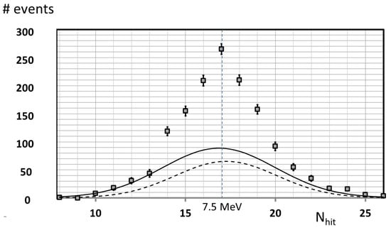
Figure 5.
Kamiokande II neutrino data on 24 February 1987. Histogram of values for 997 events in Figure 4 in ref. [33]. is the number of photomultipliers hit and is a proxy for the neutrino energy. The solid and dashed curves are two versions of the background for the detector. The dashed one was extracted from published data on a search for solar neutrinos—see Appendix A in ref. [29] for details. The solid background curve is based on a fit to this data using a Gaussian for the ten data points with and The value corresponds to MeV.
Among the reasons for being suspicious about the existence of the 8 MeV neutrino line depicted in Figure 5 is that some of the eight 17 min time intervals that contributed data were before (when the main neutrino burst occurred), and some were hours afterwards, and there was no difference in the excess counts above background for these various data subsets. Because of this lack of variation in signal strength it was concluded in ref. [35] that if the 8 MeV line were real then its luminosity would need to last over a time interval of one day. Such a long emission time is not part of any standard supernova model, but it might be possible if a significant component of the precursor star were made of dark matter, which could play a significant role in the core collapse [36]. Recall that the 8 MeV line was claimed to be due to XX annihilation, and of course dark matter heats up and cools down much more slowly than normal matter.
For the remainder of this paper, let us assume the background shown in Figure 5 is correct and the 8 MeV line is real, in which case it would have a statistical significance of around 30 sigma, although of course no such claim can be made without knowing the background shown is correct. Since the data shown is from , if the same luminosity were present for an entire day, the statistical significance of the neutrino line would become times greater had a one-day interval been examined, i.e., about 100 sigma.
4. Extragalactic Supernova Bursts
The physics and astronomy world eagerly awaits the next supernova in our galaxy. Such an event will either validate the model or alternatively show that it was an absurd fantasy of the author. There is also the possibility of observing a neutrino burst from an extragalactic supernova. Although about 20,000 extragalactic supernovae are observed each year visually, no neutrino bursts have yet been seen from these sources, given their great distances. For example, the nearest large galaxy outside our own is Andromeda, which at is 15 times further than SN 1987A was. Thus, any signal from SNe in Andromeda would be 225 times less due to the inverse square law. Even with Super-Kamiokande being 16 times the mass of Kamiokande II, a neutrino signal of the strength of SN 1987A would be roughly 14 times weaker, and presumably undetectable. Recall that for SN 1987A, ten events were recorded in a 10 s interval, so for a supernova in Andromeda, we might see one or two neutrinos in that same time window, which would be indistinguishable from background.
On the other hand, there are many dwarf and satellite galaxies closer than Andromeda, so it makes sense to look for evidence of possible neutrino bursts that might be present in existing detectors. One recent search using Super-Kamiokande IV, however, yielded only upper limits on the rate of SNe [37]. In this search for event clusters in time, they used three time windows, the longest of which was 10 s, and found no clear candidate for an extragalactic supernova neutrino burst, after weeding out imposters from about 150,000 initial clusters with a variety of cuts. Two other searches for supernova neutrino bursts conducted using the LVD detector [38] and the Baksan detector [39] also found only upper limits for neutrino clusters using time windows of 100 and 20 s, respectively.
4.1. Search for a Day-Long Burst
The possibility that the 8 MeV neutrino line is real with a luminosity lasting around a day suggests the need for a new look at previously published data using a 1-day time window to look for event clusters. Given the large number of spurious background clusters found with searches using seconds long time windows, it would be wise to use a strict screening criterion when searching for day-long clusters—perhaps selecting only ones that had a five sigma excess over the average number of neutrinos observed in one day. It is useful to estimate the distance out to which one might expect to see a five-sigma neutrino signal in a one-day time window, and to compare this with the time windows previously used in an actual search.
Suppose we have a signal of S neutrinos created from a supernova at a distance The signal is recorded with a background of B neutrinos in a detector of mass Its statistical significance would be where H (for hypernova) allows us to boost the signal strength by some factor for these more luminous supernovae. Based on the inverse square law we can express the statistical significance of a detection in terms of the detector mass background , and statistical significance for the SN 1987A observation as:
so that:
In the preceding equation or 10 depending on whether the core collapse is a supernova or a hypernova, whose luminosity is 10 to 100 times greater, due its large-mass precursor star (). In Equations (4) and (5) since Kamiokande II observed 10 neutrinos in a time window of 10 s when approximately 2 would be expected, based on Figure 4 of Hirata et al. [33]. Using Equation (5), we show in Table 1 the distance in Mly for which a supernova could be observed with the same significance as SN 1987A.

Table 1.
The distance r in million light-years (Mly) at which a supernova (SN) or hypernova (HN) could be detected in Super-Kamiokande (SK) or in Hyper-Kamiokande (HK) with the same statistical significance as SN 1987A was found with Kamiokande II. Two time windows are shown: 10 s, and 1 day.
The 8 rows of Table 1 are for both hypernovae and supernovae, for both a future (20 times larger) Hyper-Kamiokande and the present Super-Kamiokande, and finally, for the conventional 10 s time window, and the postulated day-long time window, based on the speculative 8 MeV neutrino line, having a day-long luminosity. For the latter case we assume
4.2. Observing Hypernovae at 4.81 Mly?
The most striking possibility in Table 1 is the observability of a hypernova as far as 4.81 Mly using existing Super-Kamiokande data with a 1 day burst time window at a level of The distance might even be as large as 11.1 Mly if one assumes a hypernova luminosity of not 10 but 100 times a typical SN, as was the case for the first HN ever observed [40]. To give a sense of the number of possible SN and HN sources within 4.81 Mly from Earth, we have to bear in mind there are roughly two supernovae per century in our galaxy, and there are 114 galaxies (many dwarfs or satellites) within 4.81 Mly of Earth. It should be noted, however, that hypernovae are rather rare events, which might occur in less than a few percent of core collapses [41].
Of course, one might expect to find a very substantial background with such a large time window as 1 day. In the case of SN 1987, Figure 5 shows that Kamiokande II recorded around 1000 events found over a two-hour period, with roughly half being the claimed 8 MeV signal and half background. Thus, in the 16-times-larger Super-Kamiokande during a one day time window with a signal, we might expect to find a background neutrino events and a signal of events for a hypernova at Were such a signal seen in the data one could test whether it is genuine by examining the spatial directions of all events in the 1-day time window, and seeing if they were concentrated along a particular direction in the sky. A candidate HN or SN might look something like Figure 6, if one were to assume that the 1600 signal events were to be centered at the direction with an angular resolution [42] and with a background of events uniformly distributed in direction. It is simplistic to assume a background evenly distributed in direction because many background events are not due to neutrinos at all, but instead background radiation and muons or instrumental effects, which might be reduced by various cuts, as ref. [42] has shown. Once such cuts are made, if the background was not uniformly distributed in direction, one could judge whether there were sky regions showing excesses by comparing the background on a given day with the days just before and after the day showing the excess. There is one other test a day-long neutrino burst would need to satisfy in order to confirm the model (with its 8 MeV neutrino line). It is necessary that the magnitude of the excess events above background having energy E falling in the interval: be greater than the excess for events outside that energy interval. In Super-Kamiokande the energy resolution at 10 MeV [42].
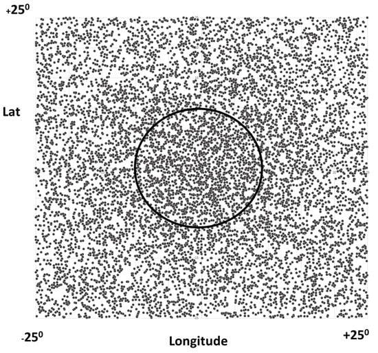
Figure 6.
Image showing 1600 simulated signal events centered at (0, 0) with a directional resolution of 18 degrees and background events uniformly distributed in (Lat, Long). The excess above the constant background inside the circle is
Even though the possibility of seeing a neutrino burst using a day-long time window may seem remote, is it not worth taking a look using existing data? Not only would such a detection be the first extragalactic neutrino burst ever seen, but it would also confirm the neutrino model, with its 8 MeV neutrino line and tachyonic neutrino mass state.
Funding
This research received no external funding.
Data Availability Statement
This research relied only on previously published data.
Acknowledgments
The author is grateful to Alan Chodos, Robert Ellsworth, Donald Gelman, and Howard “Flash” Gordon for their helpful comments.
Conflicts of Interest
The author declares no conflict of interest.
Appendix A. More Support for the Explanation of the Ankle
If the interpretation of the ankle of the spectrum is correct, namely undecayed protons reaching Earth from more and more distant sources due to time dilation at energies above the ankle, several things would have to be true. First, those highest-energy cosmic rays should have some residual anisotropy associated with their sources lying on the linear segment of the Virgo cluster. This “local” cluster contains 2000 galaxies and terminates at the Milky Way (at 11 o’clock in Figure 2). According to the Pierre Auger Collaboration, the data for cosmic rays having an energy above the ankle do in fact show a small-scale anisotropy, but the direction to the source for a maximum number of excess cosmic rays is model-dependent. According to Allard et al. for the model known as “JF12 + Planck GMF”, the direction of excess events does appear to come from the direction of the Virgo galaxy cluster—see Figure 2 in ref. [43]. It is unsurprising that their other model used shows a different source direction since their “Sun + Planck GMF” model strongly de-magnifies the sources in the Virgo direction.
If our interpretation of the ankle is correct, this should also have an observable consequence regarding the change in spectral index at the ankle. It turns out that the linear shape of the Virgo cluster almost all the way from the Milky Way out to the GZK cut-off may play a key role in this regard. If the gain in flux times after the ankle is due to undecayed protons reaching Earth from more and more distant sources, and if those sources lie along the linear segment of the Virgo cluster in Figure 2, then their number increases in proportion to the first power of their distance, and hence the first power of energy (since the mean free path before decay is proportional to the energy). Thus, if the spectrum before the ankle is a power law the added protons from more distant sources would lead to a spectrum after the ankle. Had the sources instead been distributed uniformly thoughout space in all directions, the result would have been To find the spectral index change at the ankle, we need to also take into account that while protons will be added from more and more distant sources, many will be removed from the spectrum due to decay, or at least be observed at lower energies because of it. This effect was what caused the change in spectral index at the energy of the first knee by about If that same proton loss is taken into account at the ankle the net change in spectral index (both gain and loss) would be: which agrees reasonably well with the actual spectral index change observed at the ankle
References
- Bilaniuk, O.M.P.; Deshpande, V.K.; Sudarshan, E.C.G. “Meta” relativity. Am. J. Phys. 1962, 30, 718. [Google Scholar] [CrossRef]
- Cawley, R.G. Neutrino mass bounds. Lett. Nuovo C 1972, 3, 523–525. [Google Scholar] [CrossRef]
- Chodos, A.; Hauser, A.I.; Kostelecký, V.A. The neutrino as a tachyon. Phys. Lett. B 1985, 150B, 6. [Google Scholar] [CrossRef]
- Ehrlich, R. A Review of Searches for Evidence of Tachyons. Symmetry 2022, 14, 1198. [Google Scholar] [CrossRef]
- Particle Data Group; Workman, R.L.; Burkert, V.D.; Crede, V.; Klempt, E.; Thoma, U.; Tiator, L.; Agashe, K.; Aielli, G.; Allanach, B.C.; et al. Review of Particle Properties. Prog. Theor. Exp. Phys. 2022, 2022, 083C01. [Google Scholar]
- Aleph Collaboration; Barate, R. An upper limit on the tau neutrino mass from three- and five-prong tau decays. Eur. Phys. J. C 1998, 2, 395–406. [Google Scholar] [CrossRef]
- Natarajan, A.; Zentner, A.R.; Battaglia, N.; Trac, H. Systematic errors in the measurement of neutrino masses due to baryonic feedback processes: Prospects for stage IV lensing surveys. Phys. Rev. D 2014, 90, 063516. [Google Scholar] [CrossRef]
- Chodos, A. Tachyons as a Consequence of Light-Cone Reflection Symmetry. Symmetry 2022, 14, 1947. [Google Scholar] [CrossRef]
- Nicasio, J.; Jentschura, U. Dispersion of Ultrarelativistic Tardyonic and Tachyonic Wave Packets on Cosmic Scales. Symmetry 2022, 14, 2596. [Google Scholar] [CrossRef]
- Rembieliński, J.; Caban, P.; Ciborowski, J. Quantum field theory of space-like neutrino. Eur. Phys. J. C 2021, 81, 716. [Google Scholar] [CrossRef]
- Radzikowski, M. CPT and Lorentz Symmetry; World Scientific: Singapore, 2010; pp. 224–228. [Google Scholar]
- Schwartz, C. A Consistent Theory of Tachyons with Interesting Physics for Neutrinos. Symmetry 2022, 14, 1172. [Google Scholar] [CrossRef]
- Chodos, A.; Kostelecky, V.A.; Potting, R.; Gates, E. Null experiments for neutrino masses. Mod. Phys. Lett. A 1992, 7, 467–476. [Google Scholar] [CrossRef]
- Ehrlich, R. Implications for the cosmic ray spectrum of a negative electron neutrino mass. Phys. Rev. D 1999, 60, 17302. [Google Scholar] [CrossRef]
- Abassi, R.U. The Cosmic Ray Energy Spectrum between 2 PeV and 2 EeV Observed with the TALE Detector in Monocular Mode. ApJ 2018, 865, 74. [Google Scholar] [CrossRef]
- Ehrlich, R. Is There a 4.5 PeV Neutron Line in the Cosmic Ray Spectrum? Phys. Rev. D 1999, 60, 73005. [Google Scholar] [CrossRef]
- Greisen, K. End to the cosmic-ray spectrum? Phys. Rev. Lett. 1966, 16, 748–750. [Google Scholar] [CrossRef]
- Zatsepin, G.T.; Kuz’min, V.A. Upper limit of the spectrum of cosmic rays. J. Exp. Theor. Phys. Lett. 1966, 4, 78–80. [Google Scholar]
- Tully, R.B.; Courtois, H.; Hoffman, Y.; Pomerede, D. The Laniakea supercluster of galaxies. Nature 2014, 513, 71–73. [Google Scholar] [CrossRef]
- Arsene, N. Cosmic ray mass composition at the knee using azimuthal fluctuations of air shower particles detected at ground by the KASCADE experiment, submitted to JCAP. arXiv 2023, arXiv:2303.09889. [Google Scholar]
- Plum, M.; The IceCube Collaboration. Measurements of Cosmic Ray Mass Composition with the IceCube Neutrino Observatory. EPJ Web Conf. 2023, 283, 02007. [Google Scholar] [CrossRef]
- Mollerach, S.; Roulet, E. Ultrahigh energy cosmic rays from a nearby extragalactic source in the diffusive regime. Phys. Rev. D 2019, 99, 103010. [Google Scholar] [CrossRef]
- Ehrlich, R. Possible evidence for a 5.86 PeV cosmic ray enhancement. arXiv 2014, arXiv:1307.3944. [Google Scholar]
- Aartsen, M.G.; The IceCube Collaboration. Observation of cosmic ray anisotropy with nine years of IceCube data. In Proceedings of the Science, 32nd Cosmic Ray Conference, Berlin, Germany, 23 July 2021. [Google Scholar]
- Ahlers, M.; Metsch, P. Origin of small-scale anisotropies in Galactic cosmic rays. Prog. Part. Nucl. Phys. 2017, 94, 184–216. [Google Scholar] [CrossRef]
- Neronov, A.; Semikoz, D. Possibility of measurement of cosmic ray electron spectrum up to 100 TeV with two-layer water Cherenkov detector array. arXiv 2021, arXiv:2102.08456. [Google Scholar]
- Jentschura, U.; Ehrlich, R. Lepton-pair Cerenkov radiation emitted by tachyonic neutrinos: Lorentz-covariant approach and IceCube data. Adv. High Energy Phys. 2016, 2016, 4764981. [Google Scholar] [CrossRef]
- Ehrlich, R. Tachyonic neutrinos and the neutrino masses. Astropart. Phys. 2013, 41, 1–6. [Google Scholar] [CrossRef]
- Ehrlich, R. The Mont Blanc neutrinos from SN 1987A: Could they have been monochromatic (8 MeV) tachyons. Astropart. Phys. 2018, 99, 21–29. [Google Scholar] [CrossRef]
- Ehrlich, R. First results of the KATRIN neutrino mass experiment and their consistency with an exotic 3 + 3 model. arXiv 2019, arXiv:1910.06158. [Google Scholar] [CrossRef]
- Vissani, F.; Rosso, A.G. On the time distribution of supernova antineutrino flux. Symmetry 2021, 13, 1851. [Google Scholar] [CrossRef]
- Ehrlich, R. Evidence for two neutrino mass eigenstates from SN 1987A and the possibility of superluminal neutrinos. Astropart. Phys. 2012, 35, 625–628. [Google Scholar] [CrossRef][Green Version]
- Hirata, K.; Kajita, T.; Koshiba, M.; Nakahata, M.; Oyama, Y.; Sato, N.; Suzuki, A.; Takita, M.; Totsuka, Y.; Kifune, T.; et al. Kamiokande result on a neutrino burst from the supernova SN 1987a. Phys. Rev. D 1988, 38, 448–458. [Google Scholar] [CrossRef] [PubMed]
- Feng, J.L.; Fornal, B.; Galon, I.; Gardner, S.; Smolinsky, J.; Tait, T.M.; Tanedo, P. Protophobic Fifth-Force Interpretation of the Observed Anomaly in Nuclear Transitions. Phys. Rev. Lett. 2016, 117, 071803. [Google Scholar] [CrossRef] [PubMed]
- Ehrlich, R. 5 Reasons to expect an 8 MeV line in the SN 1987A neutrino spectrum. arXiv 2021, arXiv:2101.08128. [Google Scholar] [CrossRef]
- Fayette, P.; Hooper, D.; Sigl, G. Constraints on light dark matter from core collapse supernovae. Phys. Rev. Lett. 2006, 96, 211302. [Google Scholar] [CrossRef] [PubMed]
- Mori1, M.; Abe, K.; Hayato, Y.; Hiraide, K.; Ieki, K.; Ikeda, M.; Imaizumi, S.; Kameda, J.; Kanemura, Y.; Kaneshima, R.; et al. Searching for Supernova Bursts in Super-Kamiokande IV. Astrophys. J. 2022, 938, 35. [Google Scholar]
- Vigorito, C.; Bruno, G.; Fulgione, W.; Molinario, A. Supernova Neutrinos search with the LVD experiment: The 2019 update. In Proceedings of the 36th International Cosmic Ray Conference, ICRC, Madison, WI, USA, 24 July 2019. [Google Scholar]
- Kochkarov, M.M.; Boliev, M.M.; Dzaparova, I.M.; Kurenya, A.N.; Novoseltsev, Y.F.; Novoseltseva, R.V.; Petkov, V.B.; Striganov, P.S.; Yanin, A.F. The Search for Neutrino Bursts at the Baksan Underground Scintillation Telescope: 37 Years of Exposure. Bull. Russ. Acad. Sci. Phys. 2019, 83, 923–926. [Google Scholar] [CrossRef]
- Bloom, J.S. The Host Galaxy of GRB 970508. Astrophys. J. 1998, 507, L25–L28. [Google Scholar] [CrossRef]
- Podsiadlowski, P.; Mazzali, P.A.; Nomoto, K.; Lazzati, D.; Cappellaro, E. The rates of hypernovae and gamma-ray bursts: Implications for their progenitors. Astrophys. J. 2004, 607, L17. [Google Scholar] [CrossRef]
- Suzuki, Y. Superkamiokande Collaboration, The Super-Kamiokande experiment. Eur. Phys. J. C 2019, 79, 298. [Google Scholar] [CrossRef]
- Allard, D.; Aublin, J.; Baret, B.; Parizot, E. What can be learnt from UHECR anisotropies observations. Astron. Astrophys. 2022, 664, A120. [Google Scholar] [CrossRef]


Disclaimer/Publisher’s Note: The statements, opinions and data contained in all publications are solely those of the individual author(s) and contributor(s) and not of MDPI and/or the editor(s). MDPI and/or the editor(s) disclaim responsibility for any injury to people or property resulting from any ideas, methods, instructions or products referred to in the content. |
© 2023 by the author. Licensee MDPI, Basel, Switzerland. This article is an open access article distributed under the terms and conditions of the Creative Commons Attribution (CC BY) license (https://creativecommons.org/licenses/by/4.0/).