A Semi-Discretization Method Based on Finite Difference and Differential Transform Methods to Solve the Time-Fractional Telegraph Equation

Abstract

The telegraph equation is a hyperbolic partial differential equation that has many applications in symmetric and asymmetric problems. In this paper, the solution of the time-fractional telegraph equation is obtained using a hybrid method. The numerical simulation is performed based on a combination of the finite difference and differential transform methods, such that at first, the equation is semi-discretized along the spatial ordinate, and then the resulting system of ordinary differential equations is solved using the fractional differential transform method. This hybrid technique is tested for some prominent linear and nonlinear examples. It is very simple and has a very small computation time; also, the obtained results demonstrate that the exact solutions are exactly symmetric with approximate solutions. The results of our scheme are compared with the two-dimensional differential transform method. The numerical results show that the proposed method is more accurate and effective than the two-dimensional fractional differential transform technique. Also, the implementation process of this method is very simple, so its computer programming is very fast.

1. Introduction

The differential transform method (DTM) is an iterative method based on Taylor’s series. DTM has been used to solve various differential equations. It was first applied to solve electrical circuit problems. After that, it was used to solve ordinary differential equations (ODEs), partial differential equations (PDEs), fuzzy PDEs, fractional-order ODEs and PDEs, systems of ODEs, systems of PDEs, differential-algebraic equations, and eigenvalue problems [1,2,3,4,5,6,7]. Additionally, fractional DTM, which is based on a generalized Taylor’s series, has been applied to solve various differential, differential-algebraic, and integral equations of fractional order [8,9,10,11,12,13,14]. In this paper, we intend to apply a combination of the finite difference (FD) and fractional differential transform (FDT) methods (FD-FDTM) to solve the one-dimensional time-fractional telegraph equation (FTE).

We consider the FTE in the following form [15,16,17]:

$$\begin{array}{cc}\hfill {\displaystyle \frac{{\partial }^{2\gamma }v(x,t)}{\partial t^{2\gamma }}}+2\lambda {\displaystyle \frac{{\partial }^{\gamma }v(x,t)}{\partial t^{\gamma }}}+\mu v(x,t)& =\nu {\displaystyle \frac{{\partial }^{2}v(x,t)}{\partial x^2}}+q(x,t),a<x<b,t\ge 0,\hfill \end{array}$$

(1)

with initial conditions

$$\begin{array}{cc}\hfill v(x,0)& =f_1\left(x\right),v_t(x,0)=f_2\left(x\right),a<x<b,\hfill \end{array}$$

(2)

and boundary conditions

$$\begin{array}{cc}\hfill v(a,t)& =g_1\left(t\right),v(b,t)=g_2\left(t\right),t\ge 0.\hfill \end{array}$$

(3)

where $0<\gamma <1$, $\lambda ,\mu ,$ and $\nu$ are arbitrary positive constants and $f_1,f_2,g_1$, and $g_2$ are known functions.

Also, ${\displaystyle \frac{{\partial }^{2\gamma }v(x,t)}{\partial t^{2\gamma }}}$ and ${\displaystyle \frac{{\partial }^{\gamma }v(x,t)}{\partial t^{\gamma }}}$ denote the Caputo fractional derivative of order $2\gamma$ and $\gamma$, respectively. The $\gamma$-order Caputo fractional derivative of the function f for $\gamma >0,n-1<\gamma <n$, is defined as follows:

$$\begin{array}{c}\hfill D_0^{\gamma }f\left(x\right)={\displaystyle \frac{1}{\Gamma (n-\gamma )}}{\int }_0^x{(x-t)}^{n-\gamma -1}{f}^{\left(n\right)}\left(t\right)dt.\end{array}$$

The telegraph equation is a hyperbolic PDE that has many applications in physics and engineering, for example, in signal analysis, random walk theory, anomalous diffusion processes, wave phenomena, and wave propagation of the electrical signal in the cable of a transmission line. Different numerical and analytical techniques have been used to solve fractional-order telegraph equations [15,16,17,18,19,20,21,22,23,24,25,26,27,28,29,30,31,32,33].

This work aims to obtain an approximate solution to the FTE (1) using a hybrid method. In 2008, a hybrid method based on the combination of DTM and FDM was presented to solve a nonlinear heat conduction differential equation [34]. Also, in 2012, some nonlinear PDEs were solved with the hybrid method [35]. Arsalan (2020) applied a hybrid scheme to solve the one-dimensional integer-order telegraph equations [36,37].

We organize the rest of the paper as follows. In Section 2, we present the FDTM and related theorems. We propose our hybrid method to solve FTE in Section 3 and prove its convergence in Section 4. Also, in Section 5, we give some examples and solve them with the proposed method, we draw a conclusion in Section 6.

2. Fractional Differential Transform Method

The fractional differential transform method (or generalized differential transform method) is based on the fractional Taylor’s formula. The $\alpha$-order fractional Taylor expansion of function $u\left(t\right)$ about point $t=t_0$ is defined as [38]

$$u\left(t\right)=\sum _{k=0}^{\infty }{\displaystyle \frac{{(t-t_0)}^{k\alpha }}{\Gamma (k\alpha +1)}}{\left({\displaystyle \frac{d^{\alpha }}{d{t}^{\alpha }}}\right)}^{k}u\left(t\right){\mid }_{t=t_0},$$

(4)

where ${\displaystyle \frac{d^{\alpha }}{d{t}^{\alpha }}}$ is the $\alpha$-order Caputo fractional derivative and ${\left({\displaystyle \frac{d^{\alpha }}{d{t}^{\alpha }}}\right)}^k=\underset{k-times}{\underbrace{{\displaystyle \frac{d^{\alpha }}{d{t}^{\alpha }}}\cdots {\displaystyle \frac{d^{\alpha }}{d{t}^{\alpha }}}}}$.

The $\alpha$-order FDT of the function $u\left(t\right)$ about $t=t_0$ is denoted by $U^{\alpha }\left(k\right)$ and defined as $U^{\alpha }\left(k\right)={\displaystyle \frac{1}{\Gamma (k\alpha +1)}}{\left({\displaystyle \frac{d^{\alpha }}{d{t}^{\alpha }}}\right)}^{k}u\left(t\right){\mid }_{t=t_0}$, and the inverse transform is $u\left(t\right)={\sum }_{k=0}^{\infty }{U}^{\alpha }\left(k\right){(t-t_0)}^{k\alpha }$ [9]. Therefore, at $t=0$, we have

$$u\left(t\right)=\sum _{k=0}^{\infty }{U}^{\alpha }\left(k\right)t^{k\alpha }=\sum _{k=0}^{\infty }{\phi }_k\left(t\right),$$

(5)

where ${\phi }_k\left(t\right)=U^{\alpha }\left(k\right)t^{k\alpha }$.

Also, the m-approximation fractional differential transform of $u\left(t\right)$ is defined as

$$U^m\left(t\right)=\sum _{k=0}^m{U}^{\alpha }\left(k\right)t^{k\alpha }=\sum _{k=0}^m{\phi }_k\left(t\right).$$

Theorem 1 

([39]). Suppose that $F^{\alpha }\left(k\right)$, $G^{\alpha }\left(k\right)$, and $H^{\alpha }\left(k\right)$ are the differential transformations of the functions $f\left(t\right)$, $g\left(t\right)$, and $h\left(t\right)$, respectively. Then we have

(a) 

if $f\left(t\right)=g\left(t\right)\pm h\left(t\right)$, then $F^{\alpha }\left(k\right)=G^{\alpha }\left(k\right)\pm H^{\alpha }\left(k\right)$,

(b) 

if $f\left(t\right)={(t-t_0)}^q$, then $F^{\alpha }\left(k\right)=\delta (k-{\displaystyle \frac{q}{\alpha }})$, where $\delta \left(k\right)=\{\begin{array}{cc}1,\hfill & ifk=0\hfill \\ 0.\hfill & ifk\ne 0\hfill \end{array}$

(c) 

if $f\left(t\right)=g\left(t\right)h\left(t\right)$, then $F^{\alpha }\left(k\right)={\sum }_{l=0}^k{G}^{\alpha }\left(l\right)H^{\alpha }(k-l)$,

Theorem 2 

([39]). Suppose that $f\left(t\right)=t^{\lambda }g\left(t\right)$, where $\lambda >-1$ and $g\left(t\right)$ has the generalized power series expansion $g\left(t\right)={\sum }_{n=0}^{\infty }{a}_n{(t-t_0)}^{n\alpha }$ with radius of convergence $R>0$, $0<\alpha \le 1$. Then

$$D_a^{\gamma }{D}_a^{\beta }f\left(t\right)=D_a^{\gamma +\beta }f\left(t\right),$$

for all $t\in (0,R)$ if:

(a) 

$\beta <\lambda +1$ and α arbitrary or

(b) 

$\beta \ge \lambda +1$, γ arbitrary, and $a_k=0$ for $k=0,1,\dots ,m-1$, where $m-1<\beta \le m$.

Theorem 3 

([39]). If $f\left(t\right)=D_{t_0}^{\gamma }g\left(t\right)$, $m-1<\gamma \le m$, and the function $g\left(t\right)$ satisfies the conditions in theorem (2), then

$$F^{\alpha }\left(k\right)={\displaystyle \frac{\Gamma (k\alpha +\gamma +1)}{\Gamma (k\alpha +1)}}{G}^{\alpha }(k+{\displaystyle \frac{\gamma }{\alpha }}).$$

3. FD-FDTM for Solving the FTE

Consider the FTE (1). If the x-derivative at $(x,t)$ is replaced by ${\displaystyle \frac{1}{h^2}}\left\{v(x-h,t)-2v(x,t)+v(x+h,t)\right\}+O\left(h^2\right)$ and x is considered as a constant, Equation (1) can be written as the following ordinary differential equation

$$\begin{array}{cc}\hfill {\displaystyle \frac{d^{2\gamma }v\left(t\right)}{d{t}^{2\gamma }}}+2\lambda {\displaystyle \frac{d^{\gamma }v\left(t\right)}{d{t}^{\gamma }}}+\mu v\left(t\right)& =\nu {\displaystyle \frac{1}{h^2}}\left\{v(x-h,t)-2v(x,t)+v(x+h,t)\right\}+O\left(h^2\right)+q(x,t).\hfill \end{array}$$

(6)

We subdivide the interval $[a,b]$ into N equal subintervals of step-length $h={\displaystyle \frac{b-a}{N}}$. Thus, the mesh points $x_i=a+ih$, $i=0,1,\dots ,N$ are obtained. Now, we write Equation (6) at the mesh point $x_i,i=1,\dots ,N-1$, along with time level t. If we discard the local truncation error $O\left(h^2\right)$ and denote $u_i\left(t\right)$ as the approximate solution of $v_i\left(t\right)=v(x_i,t)$, we have the following system of ODEs:

$$\begin{array}{cc}\hfill {\displaystyle \frac{d^{2\gamma }{u}_i\left(t\right)}{d{t}^{2\gamma }}}+2\lambda {\displaystyle \frac{d^{\gamma }{u}_i\left(t\right)}{d{t}^{\gamma }}}+\mu u_i\left(t\right)& ={\displaystyle \frac{\nu }{h^2}}\left\{u_{i-1}\left(t\right)-2u_i\left(t\right)+u_{i+1}\left(t\right)\right\}+q_i\left(t\right),i=1,\dots ,N-1.\hfill \end{array}$$

(7)

We solve the system (7) using FDTM. For this purpose, we consider the solution of equation, $u_i\left(t\right)$, as follows:

$$u_i\left(t\right)=\sum _{k=0}^{\infty }{U}_i^{\alpha }\left(k\right)t^{k\alpha },$$

(8)

where the unknown coefficients $U_i^{\alpha }\left(k\right)$ are the FDT of $u_i\left(t\right)$ and should be obtained.

By choosing a suitable value for $\alpha$, assuming $q_i^{\alpha }\left(k\right)$ as the $\alpha$-fractional differential transform of $q_i\left(t\right)$, and by using Theorems 2 and 3, the fractional differential transform of Equation (7) leads to the following relation:

$$\begin{array}{c}\hfill {\displaystyle \frac{\Gamma (k\alpha +2\gamma +1)}{\Gamma (k\alpha +1)}}{U}_i^{\alpha }(k+{\displaystyle \frac{2\gamma }{\alpha }})+2\lambda {\displaystyle \frac{\Gamma (k\alpha +\gamma +1)}{\Gamma (k\alpha +1)}}{U}_i^{\alpha }(k+{\displaystyle \frac{\gamma }{\alpha }})+\mu U_i^{\alpha }\left(k\right)=\\ \hfill {\displaystyle \frac{\nu }{h^2}}\{U_{i-1}^{\alpha }\left(k\right)-2U_i^{\alpha }\left(k\right)+U_{i+1}^{\alpha }\left(k\right)\}+q_i^{\alpha }\left(k\right).\end{array}$$

(9)

Now, suppose that $G_1^{\alpha }\left(k\right)$ and $G_2^{\alpha }\left(k\right)$ are the fractional differential transforms of the functions $g_1\left(t\right)$ and $g_2\left(t\right)$, respectively. Therefore, by applying the FDTM to conditions (2) and (3), we have the initial conditions

$$\begin{array}{c}\hfill U_i^{\alpha }\left(0\right)=f_1\left(x_i\right),\\ \hfill U_i^{\alpha }\left({\displaystyle \frac{1}{\alpha }}\right)=f_2\left(x_i\right),\end{array}$$

(10)

and the boundary conditions

$$\begin{array}{c}\hfill U_0^{\alpha }\left(k\right)=G_1^{\alpha }\left(k\right),\\ \hfill U_N^{\alpha }\left(k\right)=G_2^{\alpha }\left(k\right),\end{array}$$

(11)

We rewrite relations (9)–(11) as follows:

$$\begin{array}{cc}\hfill U_i^{\alpha }(k+{\displaystyle \frac{2\gamma }{\alpha }})={\displaystyle \frac{\Gamma (k\alpha +1)}{\Gamma (k\alpha +2\gamma +1)}}& \left[\nu {\displaystyle \frac{U_{i-1}^{\alpha }\left(k\right)-2U_i^{\alpha }\left(k\right)+U_{i+1}^{\alpha }\left(k\right)}{h^2}}-\mu U_i^{\alpha }\left(k\right)+q_i^{\alpha }\left(k\right)\right]\hfill \end{array}$$

$$\begin{array}{c}\hfill -2\lambda {\displaystyle \frac{\Gamma (k\alpha +\gamma +1)}{\Gamma (k\alpha +2\gamma +1)}}{U}_i^{\alpha }(k+{\displaystyle \frac{\gamma }{\alpha }}),\forall k\ge 0\end{array}$$

(12)

$$\begin{array}{c}\hfill U_i^{\alpha }\left(0\right)=f_1\left(ih\right),\\ \hfill U_i^{\alpha }\left({\displaystyle \frac{1}{\alpha }}\right)=f_2\left(ih\right),\end{array}$$

(13)

$$\begin{array}{c}\hfill U_0^{\alpha }\left(k\right)=G_1^{\alpha }\left(k\right),\\ \hfill U_N^{\alpha }\left(k\right)=G_2^{\alpha }\left(k\right).\end{array}$$

(14)

Also, according to [9], the unknown coefficients $U_i^{\alpha }\left(1\right),U_i^{\alpha }\left(2\right),\dots ,U_i^{\alpha }({\displaystyle \frac{2\gamma }{\alpha }}-1)$, will be available as follows:

$$U_i^{\alpha }\left(k\right)=\left\{\begin{array}{c}{\displaystyle \frac{1}{\Gamma (k\alpha +1)}}{\left[{\displaystyle \frac{d^{k\alpha }}{d{t}^{k\alpha }}}{u}_i\left(t\right)\right]}_{t=0},\mathrm{if}k\alpha \in {\mathbb{Z}}^{+}\hfill \\ \hfill & \forall k=0,1,\dots ({\displaystyle \frac{2\gamma }{\alpha }}-1).\hfill \\ 0,\mathrm{if}k\alpha \notin {\mathbb{Z}}^{+}\hfill \end{array}\right.$$

(15)

Therefore, all the unknown coefficients $U_i^{\alpha }\left(k\right),i=0,1,2,\dots ,N$,$\forall k\ge 0$ are calculated according to the recursive formula (12) and relations (13)–(15).

4. Convergence of FD-FDTM for FTE

Here, we discuss the convergence of FD-FDTM for solving the FTE (1). First, we present the following lemma [40].

Lemma 1. 

Suppose that for some $k_0\in {\mathbb{N}}_0$ and for every $j\ge k_0$, there exist $0<{\delta }_j<1$ such that $\parallel {\phi }_{j+1}\parallel \le {\delta }_{j+1}\parallel {\phi }_j\parallel$, $(\parallel {\phi }_j\parallel =ma{x}_t|{\phi }_j\left(t\right)\left|\right)$. Then the series ${\sum }_{k=0}^{\infty }{\phi }_k\left(t\right)$ converges to $u\left(t\right)$.

Proof. 

Consider the sequence $s_0,s_1,s_2,\dots$, where $s_n={\sum }_{k=0}^n{\phi }_k\left(t\right)$. To prove the lemma, we show the sequence $s_n$ is a Cauchy sequence in $(C\left[[0,1]\right],\parallel .{\parallel }_{\infty })$.

For $0<{\delta }_j<1$, we can write

$$\parallel s_j-s_{j-1}\parallel = \parallel {\phi }_j\parallel \le {\delta }_j\parallel {\phi }_{j-1}\parallel \le {\delta }_j{\delta }_{j-1}\parallel {\phi }_{j-2}\parallel \le \dots \le {\delta }_j{\delta }_{j-1}\dots {\delta }_{k_0}\parallel {\phi }_{k_0}\parallel ,$$

Thus, for $n\ge m\ge k_0$, we have

$$\parallel s_n-s_m\parallel = \parallel \sum _{j=m+1}^n(s_j-s_{j-1})\parallel \le \sum _{j=m+1}^n\parallel s_j-s_{j-1}\parallel \le \sum _{j=m+1}^n{\delta }_j{\delta }_{j-1}\dots {\delta }_{k_0}\parallel {\phi }_{k_0}\parallel ,$$

If we let $\delta =max\{{\delta }_{k_0},{\delta }_{k_0+1},\dots ,{\delta }_m,{\delta }_{m+1},\dots ,{\delta }_n\}$, the following relation is obtained:

$$\parallel s_n-s_m\parallel \le \sum _{j = m+1}^n{\delta }^{j-k_0+1}\parallel {\phi }_{k_0}\parallel \le \parallel {\phi }_{k_0}\parallel {\delta }^{m-k_0+2}\left[1+\delta +{\delta }^2+\cdots +{\delta }^{n-m-1}\right]={\displaystyle \frac{1-{\delta }^{n-m}}{1-\delta }}{\delta }^{m-k_0+2}\parallel {\phi }_{k_0}\parallel .$$

(16)

Since $0\le \delta <1$, we can derive ${lim}_{n,m\to \infty }\parallel s_n-s_m\parallel =0$, which means ${\left\{s_n\right\}}_{n=0}^{\infty }$ is a Cauchy sequence in $(C\left[I\right],\parallel .{\parallel }_{\infty })$. Since the space $C\left[I\right]$ with ${\parallel .\parallel }_{\infty }$ is a Banach space, we can derive that the series ${\sum }_{k=0}^{\infty }{\phi }_k\left(t\right)$ is convergent to $u\left(t\right)$. □

Theorem 4. 

Suppose that $v(x_i,t)$ is the exact solution of the FTE at point $(x_i,t),u_i\left(t\right)$ is the exact solution of Equation (7), and $U_i^m\left(t\right)={\sum }_{k=0}^m{\phi }_k\left(t\right)$, is the m-approximation of $u_i\left(t\right)$ as the approximate solution of FTE at point $(x_i,t)$. Also, suppose for some $k_0\in {\mathbb{N}}_0$ and for every $n\ge m\ge k_0,\exists 0<{\delta }_i<1$, such that $\parallel {\phi }_{i+1}\parallel \le {\delta }_{i+1}\parallel {\phi }_i\parallel$, where $\parallel {\phi }_i\parallel =ma{x}_t\left|{\phi }_i\left(t\right)\right|$. Then the solution $U_i^m\left(t\right)$ converges to the exact solution, $v_i\left(t\right)$, as $m\to \infty$. Furthermore, for some $a<\xi <b$ the maximum absolute error of the m-series, $U_i^m\left(t\right)$, as an approximation of the FTE’s exact solution satisfies the following relation:

$$\parallel v(x_i,t)-U_i^m\left(t\right)\parallel \le {\displaystyle \frac{h^2}{12}}{\displaystyle \frac{{\partial }^{4}u(\xi ,t)}{\partial x^4}}+{\displaystyle \frac{1}{1-\delta }}{\delta }^{m-k_0+2}\parallel {\phi }_{k_0}\parallel ,$$

where $\delta =max\{{\delta }_{k_0},{\delta }_{k_0+1},\dots ,{\delta }_n\}$.

Proof. 

We can write

$$\parallel v(x_i,t)-U_i^m\left(t\right)\parallel = \parallel v(x_i,t)-u_i\left(t\right)+u_i\left(t\right)-U_i^m\left(t\right)\parallel \le \parallel v(x_i,t)-u_i\left(t\right)\parallel + \parallel u_i\left(t\right)-U_i^m\left(t\right)\parallel ,$$

(17)

where $v(x_i,t)$ and $u_i\left(t\right)$ are the solutions of Equations (6) and (7), respectively.

Also, Equation (6) has been obtained by replacing the second x-derivative of $v(x,t)$ with the central FD formula in Equation (1). Therefore, for some $a<\xi <b$ we can write

$$\parallel v(x_i,t)-u_i\left(t\right)\parallel \le {\displaystyle \frac{h^2}{12}}{\displaystyle \frac{{\partial }^{4}u(\xi ,t)}{\partial x^4}}$$

(18)

From relation (16), for $n\ge m\ge k_0$, we have

$$\parallel s_n-s_m\parallel \le {\displaystyle \frac{1-{\delta }^{n-m}}{1-\delta }}{\delta }^{m-k_0+2}\parallel {\phi }_{k_0}\parallel ,$$

and since $0\le \delta <1$, then $1-{\delta }^{n-m}<1$, so we have

$$\parallel s_n-s_m\parallel \le {\displaystyle \frac{1}{1-\delta }}{\delta }^{m-k_0+2}\parallel {\phi }_{k_0}\parallel .$$

If n approaches ∞, then $s_n\to u_i\left(t\right)$ and we have

$$\parallel u_i\left(t\right)-s_m\parallel \le {\displaystyle \frac{1}{1-\delta }}{\delta }^{m-k_0+2}\parallel {\phi }_{k_0}\parallel ,$$

in the other words,

$$\parallel u_i\left(t\right)-U_i^m\left(t\right)\parallel \le {\displaystyle \frac{1}{1-\delta }}{\delta }^{m-k_0+2}\parallel {\phi }_{k_0}\parallel .$$

(19)

By replacing relations (18) and (19) in relation (17), the theorem is proved. □

5. Numerical Examples

In this section, we give some examples to show the efficiency and convenience of the mentioned method. The examples include linear and non-linear FTEs. We present the results of FD-FDTM for solving the examples and calculate the maximum absolute error (MAE) for different values of N using the following formula:

$$\begin{array}{c}\hfill E\left(N\right)=\underset{1\le i\le N}{max}|v(x_i,t)-U_i^m\left(t\right)|.\end{array}$$

Also, we compare the results of FD-FDTM with two-dimensional FDTM (2D-FDTM). Moreover, we obtain the rate of convergence (ROC) of FD-FDTM with the following formula:

$$\begin{array}{c}\hfill ROC={log}_2\left(\frac{E\left(N\right)}{E\left(2N\right)}\right).\end{array}$$

Example 1. 

Consider the following linear FTE [30]:

$$\begin{array}{cc}\hfill {\displaystyle \frac{{\partial }^{2\gamma }v(x,t)}{\partial t^{2\gamma }}}+2{\displaystyle \frac{{\partial }^{\gamma }v(x,t)}{\partial t^{\gamma }}}+v(x,t)& ={\displaystyle \frac{{\partial }^{2}v(x,t)}{\partial x^2}},0<\gamma <1,0<x<1,t>0,\hfill \end{array}$$

(20)

with the following conditions

$$\begin{array}{cc}\hfill v(x,0)& =e^x,v_t(x,0)=-2e^x,\hfill \end{array}$$

(21)

$$\begin{array}{cc}\hfill v(0,t)& =e^{-2t},v(1,t)=e^{1-2t},\hfill \end{array}$$

(22)

which has the exact solution $v(x,t)=e^{x-2t}$ for $\gamma =1$.

We describe the mentioned method to solve Equations (20)–(22) for $\gamma =0.75$, $\alpha =0.25$, and $h=0.1$ ($N=10$). Using Theorem 3, we can obtain the differential transform of the derivatives in Equation (20) as follows:

$$\begin{array}{cc}\hfill {\displaystyle \frac{{\partial }^{1.5}v(x,t)}{\partial t^{1.5}}}& \to {\displaystyle \frac{\Gamma (0.25k+2.5)}{\Gamma (0.25k+1)}}{U}_i^{0.25}(k+6),\hfill \\ \hfill {\displaystyle \frac{{\partial }^{0.75}v}{\partial t^{0.75}}}& \to {\displaystyle \frac{\Gamma (0.25k+1.75)}{\Gamma (0.25k+1)}}{U}_i^{0.25}(k+3),\hfill \\ \hfill v(x,t)& \to U_i^{0.25}\left(k\right),\hfill \\ \hfill {\displaystyle \frac{{\partial }^{2}v}{\partial x^2}}& \to {\displaystyle \frac{U_{i-1}^{0.25}\left(k\right)-2U_i^{0.25}\left(k\right)+U_{i+1}^{0.25}\left(k\right)}{h^2}}.\hfill \end{array}$$

According to relation (13), for the initial conditions we have

$$\begin{array}{cc}\hfill v(x,0)=e^x& \to U_i^{0.25}\left(0\right)=e^{x_i},\forall i=0,1,\dots ,10,\hfill \\ \hfill v_t(x,0)=-2e^x& \to U_i^{0.25}\left(4\right)=-2e^{x_i},\forall i=0,1,\dots ,10,\hfill \end{array}$$

and according to relation (15), we have

$$\begin{array}{cc}\hfill U_i^{0.25}\left(1\right)=U_i^{0.25}\left(2\right)=U_i^{0.25}\left(3\right)=U_i^{0.25}\left(5\right)=0,& \forall i=0,1,2,\dots ,10.\hfill \end{array}$$

Also, we use relation (14) for the boundary conditions, and for the right side of these relations, we use the FDT of the $e^{-2t}$, $e^{1-2t}$ functions, so we obtain

$$v(0,t)=e^{-2t}\to U_0^{0.25}\left(k\right)=\left\{\begin{array}{ccc}{\displaystyle \frac{{(-2)}^{{\displaystyle \frac{k}{4}}}}{\Gamma ({\displaystyle \frac{k}{4}}+1)}},\hfill & if{\displaystyle \frac{k}{4}}\in {\mathbb{Z}}^{+}& \\ & & \forall k\ge 0\hfill \\ 0.\hfill & if{\displaystyle \frac{k}{4}}\notin {\mathbb{Z}}^{+}\hfill & \end{array}\right.$$

$$v(1,t)=e^{1-2t}\to U_{10}^{0.25}\left(k\right)=\left\{\begin{array}{cccc}e\times {\displaystyle \frac{{(-2)}^{{\displaystyle \frac{k}{4}}}}{\Gamma ({\displaystyle \frac{k}{4}}+1)}},\hfill & if& {\displaystyle \frac{k}{4}}\in {\mathbb{Z}}^{+}& \\ & & & \forall k\ge 0\hfill \\ 0.\hfill & if\hfill & {\displaystyle \frac{k}{4}}\notin {\mathbb{Z}}^{+}\hfill & \end{array}\right.$$

By replacing the above relations in Equation (20), we obtain the following recursive relationship:

$$\begin{array}{cc}\hfill U_i^{0.25}(k+6)={\displaystyle \frac{\Gamma (0.25k+1)}{\Gamma (0.25k+2.5)}}& \left[{\displaystyle \frac{U_{i-1}^{0.25}\left(k\right)-2U_i^{0.25}\left(k\right)+U_{i+1}^{0.25}\left(k\right)}{h^2}}-U_i^{0.25}\left(k\right)\right]\hfill \\ & -2{\displaystyle \frac{\Gamma (0.25k+1.75)}{\Gamma (0.25k+2.5)}}{U}_i^{0.25}(k+3).\forall i\ge 1\hfill \end{array}$$

Thus, the solution in $(x_i,t)$, $i=0,1,\cdots ,10$ is obtained as follows:

$$\begin{array}{cc}\hfill x_0=0,u_0\left(t\right)& =\sum _{k=0}^{\infty }{U}_0^{0.25}\left(k\right)t^{0.25k}=U_0^{0.25}\left(0\right)+U_0^{0.25}\left(1\right)t^{0.25}+U_0^{0.25}\left(2\right)t^{0.5}+U_0^{0.25}\left(3\right)t^{0.75}+U_0^{0.25}\left(4\right)t+\dots ,\hfill \\ \hfill & =1+0t^{0.25}+0t^{0.5}+0t^{0.75}-2t+\dots ,\hfill \\ \hfill x_1=0.1,u_1\left(t\right)& =\sum _{k=0}^{\infty }{U}_1^{0.25}\left(k\right)t^{0.25k}=U_1^{0.25}\left(0\right)+U_1^{0.25}\left(1\right)t^{0.25}+U_1^{0.25}\left(2\right)t^{0.5}+U_1^{0.25}\left(3\right)t^{0.75}+U_1^{0.25}\left(4\right)t+\dots \hfill \\ \hfill & =e^{0.1}+0t^{0.25}+0t^{0.5}+0t^{0.75}-2e^{0.1}t+\dots ,\hfill \\ \hfill & ⋮\hfill \\ \hfill x_{10}=1,u_{10}\left(t\right)& =\sum _{k=0}^{\infty }{U}_{10}^{0.25}\left(k\right)t^{0.25k}=U_{10}^{0.25}\left(0\right)+U_{10}^{0.25}\left(1\right)t^{0.25}+U_{10}^{0.25}\left(2\right)t^{0.5}+U_{10}^{0.25}\left(3\right)t^{0.75}+U_{10}^{0.25}\left(4\right)t+\dots ,\hfill \\ \hfill & =e+0t^{0.25}+0t^{0.5}+0t^{0.75}-2et+\dots .\hfill \end{array}$$

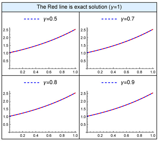
We show the results of our method for solving Example 1 in Table 1 and Table 2. Table 1 contains the maximum absolute error of the obtained solution using the FD-FDTM for $\gamma =1$, $m=3$, and different values of N at $t=0.001$. Also, we compared the results of FD-FDTM with two-dimensional FDTM. Table 1 shows the our method is more accurate than the two-dimensional DTM. Also, we can see that as N increases, the error decreases and the numerical ROC confirms the theoretical ROC. Table 2 compares the approximate solution of FD-FDTM and 2D-FDTM at $t=0.01$, for $\gamma =0.75$, $m=10$, and $N=10$. Figure 1 shows the comparison between the exact solution for $\gamma =1$ and the results of FD-FDTM for $\gamma =0.5,0.7,0.8,0.9$.

Table 1. The MAE for Example 1 at $t=0.001$, for $\gamma =1$, $m=3$, and different values of N.

N	$\mathbf{MAE}\mathbf{of}\mathbf{FD}$-$\mathbf{FDTM}(\mathit{\gamma }=1)$	ROC	$\mathbf{CPU}\mathbf{Time}$	$\mathbf{MAE}\mathbf{of}2\mathbf{D}$-$\mathbf{DTM}(\mathit{\gamma }=1)$	$\mathbf{CPU}\mathbf{Time}$
	$\mathbf{for}\mathit{\alpha }=\mathbf{1}$			$\mathbf{for}\mathit{\alpha }=\mathbf{1}$
10	$1\times {10}^{-9}$	—	$0.11$	$3.3\times {10}^{-2}$	$0.09$
20	$2.7\times {10}^{-10}$	1.89	$0.11$	$4.1\times {10}^{-2}$	$0.09$
40	$6.7\times {10}^{-11}$	2.01	$0.11$	$4.6\times {10}^{-2}$	$0.09$
80	$1.5\times {10}^{-11}$	2.16	$0.11$	$4.8\times {10}^{-2}$	$0.11$
160	$2.6\times {10}^{-12}$	2.51	$0.16$	$5.01\times {10}^{-2}$	$0.14$

Table 2. The approximate solution of Example 1 obtained with FD-FDTM and 2D-FDTM at $t=0.01$, for $\gamma =0.75$, $\alpha =0.25$, $m=10$, and $N=10$.

${\mathit{x}}_{\mathit{i}}$	FD-FDTM	2D-FDTM	$\mathbf{Exact} \mathbf{Solution}$
	$\mathit{\gamma }=\mathbf{0.75}$	$\mathit{\gamma }=\mathbf{0.75}$	$\mathit{\gamma }=\mathbf{1}$
$0.1$	$1.08391073378$	$1.08391006915$	$1.08328706767$
$0.2$	$1.19790662077$	$1.19790588623$	$1.19721736312$
$0.3$	$1.32389155984$	$1.32389074805$	$1.32312981233$
$0.4$	$1.46312645063$	$1.46312555346$	$1.46228458943$
$0.5$	$1.617004802$	$1.61700381117$	$1.61607440219$
$0.6$	$1.7870666823$	$1.7870655864$	$1.78603843075$
$0.7$	$1.9750141259$	$1.9750129144$	$1.9738777322$
$0.8$	$2.1827281748$	$2.1827268341$	$2.1814722654$
$0.9$	$2.41228770087$	$2.412286213$	$2.4108997064$

Figure 1. Comparison between the exact solution of Example 1 for $\gamma =1$ and numerical solutions for $\gamma =0.5,0.7,0.8,0.9$.

Example 2. 

In this example, we consider a non-homogeneous FTE [17]

$$\begin{array}{c}\hfill {\displaystyle \frac{{\partial }^{2\gamma }v(x,t)}{\partial t^{2\gamma }}}+40{\displaystyle \frac{{\partial }^{\gamma }v(x,t)}{\partial t^{\gamma }}}+100v(x,t)={\displaystyle \frac{{\partial }^{2}v(x,t)}{\partial x^2}}+23e^{-2t}sinh\left(x\right),0<\gamma <1,0<x<1,t>0,\end{array}$$

(23)

with the following conditions:

$$\begin{array}{c}\hfill v(x,0)=sinh\left(x\right),v_t(x,0)=-2sinh\left(x\right),\end{array}$$

(24)

$$\begin{array}{c}\hfill v(0,t)=0,v(1,t)=e^{-2t}sinh\left(1\right).\end{array}$$

(25)

The exact solution of (23) for $\gamma =1$ with conditions (24) and (25) is $v(x,t)=e^{-2t}sinh\left(x\right)$.

For example, we put $\gamma =0.6$ in (23) and consider $h=0.1$ and $\alpha =0.1$. For these values of $\gamma ,h$, and α, we can write

$$\begin{array}{cc}\hfill {\displaystyle \frac{{\partial }^{1.2}v(x,t)}{\partial t^{1.2}}}& \to {\displaystyle \frac{\Gamma (0.1k+2.2)}{\Gamma (0.1k+1)}}{U}_i^{0.1}(k+12),\hfill \\ \hfill {\displaystyle \frac{{\partial }^{0.6}v}{\partial t^{0.6}}}& \to {\displaystyle \frac{\Gamma (0.1k+1.6)}{\Gamma (0.1k+1)}}{U}_i^{0.1}(k+6),\hfill \\ \hfill v(x,t)& \to U_i^{0.1}\left(k\right),\hfill \\ \hfill {\displaystyle \frac{{\partial }^{2}v}{\partial x^2}}& \to {\displaystyle \frac{U_{i-1}^{0.1}\left(k\right)-2U_i^{0.1}\left(k\right)+U_{i+1}^{0.1}\left(k\right)}{h^2}}.\hfill \end{array}$$

According to relation (13), for the initial conditions we have:

$$\begin{array}{cc}\hfill v(x,0)=sinh\left(x\right)& \to U_i^{0.1}\left(0\right)=sinh\left(x_i\right),\forall i=0,1,2,\dots ,10,\hfill \\ \hfill v_t(x,0)=-2sinh\left(x\right)& \to U_i^{0.1}\left(10\right)=-2sinh\left(x_i\right),\forall i=0,1,2,\dots ,10,\hfill \end{array}$$

and according to (15), we have

$$\begin{array}{cc}\hfill U_i^{0.1}\left(1\right)=U_i^{0.1}\left(2\right)=\dots =U_i^{0.1}\left(9\right)=U_i^{0.1}\left(11\right)=0,& \forall i=0,1,\dots ,10.\hfill \end{array}$$

We use relation (14) for the boundary conditions, and for the right side of the boundary conditions, we use the FDT of the $e^{-2t}sinh\left(1\right)$ function. Therefore, we have

$$v(0,t)=0\to U_0^{0.1}\left(k\right)=0,\forall k\ge 0$$

$$U_{10}^{0.1}\left(k\right)=\left\{\begin{array}{cc}sinh\left(1\right)\times {\displaystyle \frac{{(-2)}^{{\displaystyle \frac{k}{10}}}}{\Gamma ({\displaystyle \frac{k}{10}}+1)}},\hfill & \hspace{1em}if\hspace{1em}{\displaystyle \frac{k}{10}}\in {\mathbb{Z}}^{+}\hfill \\ \hspace{1em}\hspace{1em}\hspace{1em}\hspace{1em}\hspace{1em}\hfill & \hspace{1em}\hspace{1em}\hspace{1em}\hspace{1em}\hspace{1em}\hspace{1em}\hspace{1em}\forall k\ge 0\hfill \\ 0.\hfill & \hspace{1em}if\hspace{1em}{\displaystyle \frac{k}{10}}\notin {\mathbb{Z}}^{+}\hfill \end{array}\right.$$

By putting the above relations in Equation (23), we conclude the following recursive relationship:

$$\begin{array}{cc}\hfill U_i^{0.1}(k+12)={\displaystyle \frac{\Gamma (0.1k+1)}{\Gamma (0.1k+2.2)}}& \left[23E^{0.1}\left(k\right)sinh\left(x_i\right)-100U_i^{0.1}\left(k\right)+{\displaystyle \frac{U_{i-1}^{0.1}\left(k\right)-2U_i^{0.1}\left(k\right)+U_{i+1}^{0.1}\left(k\right)}{h^2}}\right]\hfill \\ \hfill & -40{\displaystyle \frac{\Gamma (0.1k+1.6)}{\Gamma (0.1k+2.2)}}{U}_i^{0.1}(k+6),\hfill \end{array}$$

where $E^{0.1}\left(k\right)$ is the fractional differential transform of $e^{-2t}$ and can be obtained as follows:

$$E^{0.1}\left(k\right)=\left\{\begin{array}{cc}{\displaystyle \frac{{(-2)}^{{\displaystyle \frac{k}{10}}}}{\Gamma ({\displaystyle \frac{k}{10}}+1)}},\hfill & \hspace{1em}if\hspace{1em}{\displaystyle \frac{k}{10}}\in {\mathbb{Z}}^{+}\hfill \\ \hspace{1em}\hspace{1em}\hspace{1em}\hspace{1em}\hspace{1em}\hfill & \hspace{1em}\hspace{1em}\hspace{1em}\hspace{1em}\hspace{1em}\hspace{1em}\hspace{1em}\forall k\ge 0\hfill \\ 0.\hfill & \hspace{1em}if\hspace{1em}{\displaystyle \frac{k}{10}}\notin {\mathbb{Z}}^{+}\hfill \end{array}\right.$$

Thus, in the points $(x_i,t),i=0,1,\cdots ,N$, we can write:

$$\begin{array}{cc}\hfill x_0=0,u_0\left(t\right)& =\sum _{k=0}^{\infty }{U}_0^{0.1}\left(k\right)t^{0.1k}=U_0^{0.1}\left(0\right)+U_0^{0.1}\left(1\right)t^{0.1}+U_0^{0.1}\left(2\right)t^{0.2}+U_0^{0.1}\left(3\right)t^{0.3}+U_0^{0.1}\left(4\right)t^{0.4}+\dots ,\hfill \\ \hfill & =0+0t^{0.1}+0t^{0.2}+0t^{0.3}+0t^{0.4}+\dots ,\hfill \\ \\ \hfill x_1=0.1,u_1\left(t\right)& =\sum _{k=0}^{\infty }{U}_1^{0.1}\left(k\right)t^{0.1k}=U_1^{0.1}\left(0\right)+U_1^{0.1}\left(1\right)t^{0.1}+U_1^{0.1}\left(2\right)t^{0.2}+\dots +U_1^{0.1}\left(9\right)t^{0.9}+U_1^{0.1}\left(10\right)t+\dots ,\hfill \\ \hfill & =sinh\left(0.1\right)+0t^{0.1}+0t^{0.2}+\dots +0t^{0.9}-2sinh\left(0.1\right)t+\dots ,\hfill \\ \hfill & ⋮\hfill \\ \hfill x_{10}=1,u_{10}\left(t\right)& =\sum _{k=0}^{\infty }{U}_{10}^{0.1}\left(k\right)t^{0.1k}=U_{10}^{0.1}\left(0\right)+U_{10}^{0.1}\left(1\right)t^{0.1}+U_{10}^{0.1}\left(2\right)t^{0.2}+\dots +U_{10}^{0.1}\left(9\right)t^{0.9}+U_{10}^{0.1}\left(10\right)t+\dots ,\hfill \\ \hfill & =sinh\left(1\right)+0t^{0.1}+0t^{0.2}+\dots +0t^{0.9}-2sinh\left(1\right)t+\dots .\hfill \end{array}$$

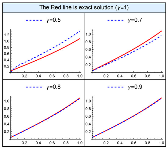
To compare the exact and numerical solution of Example 2 obtained using FD-FDTM and 2D-FDTM, we compute the MAE of the obtained solution at $t=0.001$, and present them in Table 3. Also, we show the results of the FD-FDTM and 2D-FDTM at $t=0.001$, for $\gamma =0.6$, $m=15$, and $N=10$ in Table 4. Figure 2 shows the comparison between the exact solution for $\gamma =1$ and the numerical solution for $\gamma =0.5,0.7,0.8,0.9$.

Table 3. The MAE for Example 2 at $t=0.001$, for $\gamma =1$, $m=3$, and different values of N.

N	$\mathbf{MAE}\mathbf{of}\mathbf{FD}$-$\mathbf{FDTM}$	ROC	$\mathbf{CPU}\mathbf{Time}$	$\mathbf{MAE}\mathbf{of}2\mathbf{D}$-$\mathbf{FDTM}$	$\mathbf{CPU}\mathbf{Time}$
	$\mathbf{for}\mathit{\alpha }=\mathbf{1}$			$\mathbf{for}\mathit{\alpha }=\mathbf{1}$
10	$4.2\times {10}^{-10}$	—	$0.11$	$9.1\times {10}^{-1}$	$0.14$
20	$1.1\times {10}^{-10}$	1.8	$0.12$	$9.5\times {10}^{-1}$	$0.12$
40	$2.8\times {10}^{-11}$	1.97	$0.11$	$9.7\times {10}^{-1}$	$0.11$
80	$6.7\times {10}^{-12}$	2.06	$0.14$	$9.8\times {10}^{-1}$	$0.11$
160	$1.09\times {10}^{-12}$	2.61	$0.17$	$9.9\times {10}^{-1}$	$0.17$

Table 4. The approximate solution for Example 2 at $t=0.001$, for $\gamma =0.6$, $\alpha =0.1$, $m=15$, and values of $N=10$.

${\mathit{x}}_{\mathit{i}}$	FD-FDTM	2D-FDTM	$\mathbf{Exact} \mathbf{Solution}$
	$\mathit{\gamma }=\mathbf{0.6}$	$\mathit{\gamma }=\mathbf{0.6}$	$\mathit{\gamma }=\mathbf{1}$
$0.1$	$0.097705$	$0.0164227$	$0.099966$
$0.2$	$0.19633389$	$0.0330099$	$0.2009337$
$0.3$	$0.297038$	$0.049763$	$0.30391186$
$0.4$	$0.40066$	$0.0666829$	$0.409931642$
$0.5$	$0.508292$	$0.083771$	$0.52005415$
$0.6$	$0.621011$	$0.101028$	$0.63538154$
$0.7$	$0.739945$	$0.118456$	$0.757068$
$0.8$	$0.866285$	$0.136056$	$0.8863315$
$0.9$	$1.0013$	$0.153829$	$1.024465743$

Figure 2. Comparison between the exact solution of Example 2 for $\gamma =1$ and numerical solutions for $\gamma =0.5,0.7,0.8,0.9$.

Example 3. 

In this example, we solve the following nonlinear FTE [23]:

$$\begin{array}{c}\hfill {\displaystyle \frac{{\partial }^{2\gamma }v(x,t)}{\partial t^{2\gamma }}}+2{\displaystyle \frac{{\partial }^{\gamma }v(x,t)}{\partial t^{\gamma }}}+u^2(x,t)={\displaystyle \frac{{\partial }^{2}v(x,t)}{\partial x^2}}+e^{2x-4t}-e^{x-2t},0<\gamma <1,0<x<1,t>0,\end{array}$$

(26)

with the following conditions

$$\begin{array}{c}\hfill v(x,0)=e^x,v_t(x,0)=-2e^x,\end{array}$$

(27)

$$\begin{array}{c}\hfill v(0,t)=e^{-2t},v(1,t)=e^{1-2t}.\end{array}$$

(28)

The exact solution of Equation (26) for $\gamma =1$ with conditions (27) and (28) is $v(x,t)=e^{x-2t}$.

To explain the FD-FDTM, we put $\gamma =0.75$ in (26) and consider $h=0.1$ and $\alpha =0.25$. For these values of $\gamma ,h$, and α, we can write

$$\begin{array}{cc}\hfill {\displaystyle \frac{{\partial }^{1.5}v(x,t)}{\partial t^{1.5}}}& \to {\displaystyle \frac{\Gamma (0.25k+2.5)}{\Gamma (0.25k+1)}}{U}_i^{0.25}(k+6),\hfill \\ \hfill {\displaystyle \frac{{\partial }^{0.75}v}{\partial t^{0.75}}}& \to {\displaystyle \frac{\Gamma (0.25k+1.75)}{\Gamma (0.25k+1)}}{U}_i^{0.25}(k+3),\hfill \\ \hfill v(x,t)& \to U_i^{0.25}(i,k),\hfill \\ \hfill {\displaystyle \frac{{\partial }^{2}v}{\partial x^2}}& \to {\displaystyle \frac{U_{i-1}^{0.25}\left(k\right)-2U_i^{0.25}\left(k\right)+U_{i+1}^{0.25}\left(k\right)}{h^2}}.\hfill \end{array}$$

According to relation (13), for the initial conditions we have

$$\begin{array}{cc}\hfill v(x,0)=e^x& \to U_i^{0.25}\left(0\right)=e^{x_i},\forall i=0,1,\dots ,10,\hfill \\ \hfill v_t(x,0)=-2e^x& \to U_i^{0.25}\left(4\right)=-2e^{x_i},\forall i=0,1,\dots ,10.\hfill \end{array}$$

From relationship (15), we can write

$$\begin{array}{c}\hfill U_i^{0.25}\left(1\right)=U_i^{0.25}\left(2\right)=U_i^{0.25}\left(3\right)=U_i^{0.25}\left(5\right)=0,\forall i=0,1,2,\dots ,10.\end{array}$$

We use relation (14) for the boundary conditions and an FDT of $e^{-2t}$, $e^{1-2t}$ for the right side of the boundary conditions. Therefore, we have

$$v(0,t)=e^{-2t}\to U_0^{0.25}\left(k\right)=\left\{\begin{array}{cc}{\displaystyle \frac{{(-2)}^{{\displaystyle \frac{k}{4}}}}{\Gamma ({\displaystyle \frac{k}{4}}+1)}},\hfill & \hspace{1em}if\hspace{1em}{\displaystyle \frac{k}{4}}\in {\mathbb{Z}}^{+}\hfill \\ \hspace{1em}\hspace{1em}\hspace{1em}\hspace{1em}\hspace{1em}\hfill & \hspace{1em}\hspace{1em}\hspace{1em}\hspace{1em}\hspace{1em}\hspace{1em}\hspace{1em}\forall k\ge 0\hfill \\ 0.\hfill & \hspace{1em}if\hspace{1em}{\displaystyle \frac{k}{4}}\notin {\mathbb{Z}}^{+}\hfill \end{array}\right.$$

$$v(1,t)=e^{1-2t}\to U_{10}^{0.25}\left(k\right)=\left\{\begin{array}{cc}e\times {\displaystyle \frac{{(-2)}^{{\displaystyle \frac{k}{4}}}}{\Gamma ({\displaystyle \frac{k}{4}}+1)}},\hfill & \hspace{1em}if\hspace{1em}{\displaystyle \frac{k}{4}}\in {\mathbb{Z}}^{+}\hfill \\ \hspace{1em}\hspace{1em}\hspace{1em}\hspace{1em}\hspace{1em}\hfill & \hspace{1em}\hspace{1em}\hspace{1em}\hspace{1em}\hspace{1em}\hspace{1em}\hspace{1em}\forall k\ge 0\hfill \\ 0.\hfill & \hspace{1em}if\hspace{1em}{\displaystyle \frac{k}{4}}\notin {\mathbb{Z}}^{+}\hfill \end{array}\right.$$

In Example 3, we have $q(x,t)=e^{2x-4t}-e^{x-2t}$, so by using FD-FDTM, we have:

$$\begin{array}{c}\hfill q_i^{0.25}\left(k\right)=e^{2x_i}\times E_1^{0.25}\left(k\right)-e^{x_i}\times E_2^{0.25}\left(k\right),\forall i=0,1,\dots ,10,\end{array}$$

where $E_1^{0.25}\left(k\right)$ and $E_2^{0.25}\left(k\right)$ are the FDT of the $e^{-4t}$ and $e^{-2t}$ functions, respectively, and are obtained as follows:

$$E_1^{0.25}\left(k\right)=\left\{\begin{array}{cc}{\displaystyle \frac{{(-4)}^{{\displaystyle \frac{k}{4}}}}{\Gamma ({\displaystyle \frac{k}{4}}+1)}},\hfill & \hspace{1em}if\hspace{1em}{\displaystyle \frac{k}{4}}\in {\mathbb{Z}}^{+}\hfill \\ \hspace{1em}\hspace{1em}\hspace{1em}\hspace{1em}\hspace{1em}\hfill & \hspace{1em}\hspace{1em}\hspace{1em}\hspace{1em}\hspace{1em}\hspace{1em}\hspace{1em}\forall k\ge 0\hfill \\ 0,\hfill & \hspace{1em}if\hspace{1em}{\displaystyle \frac{k}{4}}\notin {\mathbb{Z}}^{+}\hfill \end{array}\right.$$

and

$$E_2^{0.25}\left(k\right)=\left\{\begin{array}{cc}{\displaystyle \frac{{(-2)}^{{\displaystyle \frac{k}{4}}}}{\Gamma ({\displaystyle \frac{k}{4}}+1)}},\hfill & \hspace{1em}if\hspace{1em}{\displaystyle \frac{k}{4}}\in {\mathbb{Z}}^{+}\hfill \\ \hspace{1em}\hspace{1em}\hspace{1em}\hspace{1em}\hspace{1em}\hfill & \hspace{1em}\hspace{1em}\hspace{1em}\hspace{1em}\hspace{1em}\hspace{1em}\hspace{1em}\forall k\ge 0\hfill \\ 0.\hfill & \hspace{1em}if\hspace{1em}{\displaystyle \frac{k}{4}}\notin {\mathbb{Z}}^{+}\hfill \end{array}\right.$$

By substituting the above relations in Equation (26), we obtain the following recursive formula

$$\begin{array}{cc}\hfill U_i^{0.25}(k+6)={\displaystyle \frac{\Gamma (0.25k+1)}{\Gamma (0.25k+2.5)}}& \left[q_i^{0.25}\left(k\right)+{\displaystyle \frac{U_{i-1}^{0.25}\left(k\right)-2U_i^{0.25}\left(k\right)+U_{i+1}^{0.25}\left(k\right)}{h^2}}-\sum _{j=0}^k{U}_i^{0.25}\left(j\right)U_i^{0.25}(k-j)\right]\hfill \\ & -2{\displaystyle \frac{\Gamma (0.25k+1.75)}{\Gamma (0.25k+2.5)}}{U}_i^{0.25}(k+3).\forall i\ge 1\hfill \end{array}$$

In the points $(x_i,t),i=0,1,\cdots ,N$, we have:

$$\begin{array}{cc}\hfill x_0=0,u_0\left(t\right)& =\sum _{k=0}^{\infty }{U}_0^{0.25}\left(k\right)t^{0.25k}=U_0^{0.25}\left(0\right)+U_0^{0.25}\left(1\right)t^{0.25}+U_0^{0.25}\left(2\right)t^{0.5}+U_0^{0.25}\left(3\right)t^{0.75}+U_0^{0.25}\left(4\right)t+\dots \hfill \\ \hfill & =1+0t^{0.25}+0t^{0.5}+0t^{0.75}-2t+\dots ,\hfill \\ \hfill x_1=0.1,u_1\left(t\right)& =\sum _{k=0}^{\infty }{U}_1^{0.25}\left(k\right)t^{0.25k}=U_1^{0.25}\left(0\right)+U_1^{0.25}\left(1\right)t^{0.25}+U_1^{0.25}\left(2\right)t^{0.5}+U_1^{0.25}\left(3\right)t^{0.75}+U_1^{0.25}\left(4\right)t+\dots \hfill \\ \hfill & =e^{0.1}+0t^{0.25}+0t^{0.5}+0t^{0.75}-2e^{0.1}t+\dots ,\hfill \\ \hfill & ⋮\hfill \\ \hfill x_{10}=1,u_{10}\left(t\right)& =\sum _{k=0}^{\infty }{U}_{10}^{0.25}\left(k\right)t^{0.25k}=U_{10}^{0.25}\left(0\right)+U_{10}^{0.25}\left(1\right)t^{0.25}+U_{10}^{0.25}\left(2\right)t^{0.5}+U_{10}^{0.25}\left(3\right)t^{0.75}+U_{10}^{0.25}\left(4\right)t+\dots \hfill \\ \hfill & =e+0t^{0.25}+0t^{0.5}+0t^{0.75}-2et+\dots .\hfill \end{array}$$

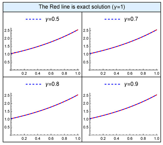
We show the results of our method for solving Example 3 in Table 5. Table 5 contains the MAE of the solution obtained using FD-FDTM, for $\gamma =1$, $m=3$, and different values of N at $t=0.01$. Also, we compared the results of FD-FDTM with two-dimensional FDTM. Table 5 shows that the FD-FDTM is more accurate than the two-dimensional FDTM. Figure 3 compares the exact solution for $\gamma =1$ with the numerical solution for $\gamma =0.5,0.7,0.8,0.9$.

Table 5. The MAE for Example 3 at $t=0.01$, for $\gamma =1$, $m=3$, and different values of N.

N	$\mathbf{MAE}\mathbf{of}\mathbf{FD}$-$\mathbf{FDTM}$	$\mathbf{CPU}\mathbf{Time}$	$\mathbf{MAE}\mathbf{of}2\mathbf{D}$-$\mathbf{DTM}$	$\mathbf{CPU}\mathbf{Time}$
	$\mathbf{for}\mathit{\alpha }=\mathbf{1}$		$\mathbf{for}\mathit{\alpha }=\mathbf{1}$
10	$7.04\times {10}^{-9}$	$0.11$	$3.1\times {10}^{-1}$	$0.11$
20	$8.64\times {10}^{-9}$	$0.12$	$4.1\times {10}^{-2}$	$0.11$
40	$9.3\times {10}^{-9}$	$0.12$	$4.62\times {10}^{-2}$	$0.11$
80	$9.59\times {10}^{-9}$	$0.16$	$4.88\times {10}^{-2}$	$0.11$
160	$9.72\times {10}^{-9}$	$0.17$	$5.01\times {10}^{-2}$	$0.12$

Figure 3. Comparison between the exact solution of Example 3 for $\gamma =1$ and numerical solutions for $\gamma =0.5,0.7,0.8,0.9$.

Example 4. 

Consider the following time-fractional multi-term wave equation [32]:

$$\begin{array}{cc}\hfill {\displaystyle \frac{{\partial }^{1.7}v(x,t)}{\partial t^{1.7}}}-{\displaystyle \frac{1}{2}}{\displaystyle \frac{\partial v(x,t)}{\partial t}}& ={\displaystyle \frac{{\partial }^{2}v(x,t)}{\partial x^2}},0<x<4,t>0,\hfill \end{array}$$

(29)

with initial conditions

$$\begin{array}{cc}\hfill v(x,0)& =sin\left(\pi x\right),v_t(x,0)=0,\hfill \end{array}$$

(30)

and boundary conditions

$$\begin{array}{cc}\hfill v(0,t)& =0,v(4,t)=0,\hfill \end{array}$$

(31)

We describe the mentioned method to solve Equations (29)–(31) for $\alpha =0.1$ By using theorem (3), we can obtain the differential transform of the derivatives in Equation (29) as follows:

$$\begin{array}{cc}\hfill {\displaystyle \frac{{\partial }^{1.7}v(x,t)}{\partial t^{1.7}}}& \to {\displaystyle \frac{\Gamma (0.1k+2.7)}{\Gamma (0.1k+1)}}{U}_i^{0.1}(k+17),\hfill \\ \hfill {\displaystyle \frac{\partial v}{\partial t}}& \to {\displaystyle \frac{\Gamma (0.1k+2)}{\Gamma (0.1k+1)}}{U}_i^{0.1}(k+10),\hfill \\ \hfill {\displaystyle \frac{{\partial }^{2}v}{\partial x^2}}& \to {\displaystyle \frac{U_{i-1}^{0.1}\left(k\right)-2U_i^{0.1}\left(k\right)+U_{i+1}^{0.1}\left(k\right)}{h^2}}.\hfill \end{array}$$

According to relation (13), for the initial conditions we have

$$\begin{array}{cc}\hfill v(x,0)=sin\left(\pi x\right)& \to U_i^{0.1}\left(0\right)=sin\left(\pi x_i\right),\forall i=0,1,\dots ,N,\hfill \\ \hfill v_t(x,0)=0& \to U_i^{0.1}\left(10\right)=0,\forall i=0,1,\dots ,N,\hfill \end{array}$$

and according to relation (15) we have

$$\begin{array}{cc}\hfill U_i^{0.1}\left(1\right)=U_i^{0.1}\left(2\right)=\dots =U_i^{0.1}\left(15\right)=U_i^{0.1}\left(16\right)=0,& \forall i=0,1,\dots ,N,\hfill \end{array}$$

and

$$\begin{array}{c}\hfill v(0,t)=0\to U_0^{0.1}\left(k\right)=0,\\ \hfill v(4,t)=0\to U_N^{0.1}\left(k\right)=0.\end{array}$$

By replacing the above relations in Equation (29), we obtain the following recursive relationship:

$$\begin{array}{cc}\hfill U_i^{0.1}(k+17)={\displaystyle \frac{\Gamma (0.1k+1)}{\Gamma (0.1k+2.7)}}& \left({\displaystyle \frac{U_{i-1}^{0.1}\left(k\right)-2U_i^{0.1}\left(k\right)+U_{i+1}^{0.1}\left(k\right)}{h^2}}\right)\hfill \\ & +{\displaystyle \frac{1}{2}}{\displaystyle \frac{\Gamma (0.1k+2)}{\Gamma (0.1k+2.5)}}{U}_i^{0.1}(k+10).\forall i\ge 1\hfill \end{array}$$

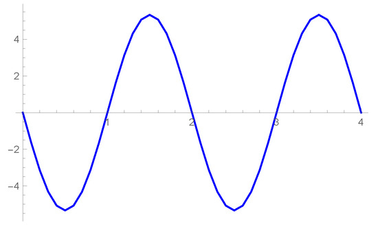
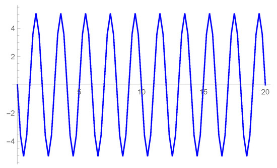
We show the results of our method for solving Example 4 in Figure 4 and Figure 5 for $t=1$.

Figure 4. Solution of Example 4 for $N=40,m=20$.

Figure 5. Solution of Example 4 for $N=80,m=20$.

6. Conclusions

In this work, a hybrid method has been used to solve the linear and non-linear time-fractional telegraph equation approximately. The central difference method has been applied to discretize the spatial derivative and the fractional differential transform method has been used to solve the obtained system of fractional ordinary equations. A convergence analysis of the mentioned method has been conducted. The numerical results show that the proposed hybrid method is more accurate and effective than two-dimensional FDTM. Also, the implementation process of this method is very simple, so its computer programming is very fast.

References

- Chen, C.K.; Ho, S.H. Application of differential transformation to eigenvalue problems. Appl. Math. Comput. 1996, 79, 173–188. [Google Scholar] [CrossRef]
- Zhou, J.K. Differential Transformation and Its Applications for Electrical Circuits; Huazhong University Press: Wuhan, China, 1986. [Google Scholar]
- Jang, M.J.; Chen, C.L.; Liy, Y.C. On solving the initial-value problems using the differential transformation method. Appl. Math. Comput. 2000, 115, 145–160. [Google Scholar] [CrossRef]
- Ayaz, F. Applications of differential transform method to differential-algebraic equations. Appl. Math. Comput. 2004, 152, 649–657. [Google Scholar] [CrossRef]
- Hassan, I.A.H. On solving some eigenvalue problems by using a differential transformation. Appl. Math. Comput. 2002, 127, 1–22. [Google Scholar]
- Alquran, M.T. Applying differential transform method to nonlinear partial differential equations: A modified approach. Appl. Appl. Math. Int. J. (AAM) 2012, 7, 10. [Google Scholar]
- Mirzaee, F.; Yari, M.K. A novel computing three-dimensional differential transform method for solving fuzzy partial differential equations. Ain Shams Eng. J. 2016, 7, 695–708. [Google Scholar] [CrossRef]
- Ertürk, V.S.; Momani, S. Solving systems of fractional differential equations using differential transform method. J. Comput. Appl. Math. 2008, 215, 142–151. [Google Scholar] [CrossRef]
- Odibat, Z.; Momani, S. A generalized differential transform method for linear partial differential equations of fractional order. Appl. Math. Lett. 2008, 21, 194–199. [Google Scholar] [CrossRef]
- Ibis, B.; Bayram, M.; Agargun, A.G. Applications of fractional differential transform method to fractional differential-algebraic equations. Eur. J. Pure Appl. Math. 2011, 4, 129–141. [Google Scholar]
- Ertürk, V.S. Computing eigenelements of Sturm–Liouville problems of fractional order via fractional differential transform method. Math. Comput. Appl. 2011, 16, 712–720. [Google Scholar] [CrossRef]
- Secer, A.; Akinlar, M.A.; Cevikel, A. Efficient solutions of systems of fractional PDEs by the differential transform method. Adv. Differ. Equ. 2012, 2012, 1–7. [Google Scholar] [CrossRef]
- Zain, F.A.S. Comparison study between differential transform method and Adomian decomposition method for some delay differential equations. Int. J. Phys. Sci. 2013, 8, 744–749. [Google Scholar]
- Rahimi, E.; Taghvafard, H.; Erjaee, G.H. Fractional differential transform method for solving a class of weakly singular Volterra integral equations. Iran. J. Sci. Technol. 2014, 38, 69. [Google Scholar]
- Hosseini, V.R.; Chen, W.; Avazzadeh, Z. Numerical solution of fractional telegraph equation by using radial basis functions. Eng. Anal. Bound. Elem. 2014, 38, 31–39. [Google Scholar] [CrossRef]
- Asghari, M.; Ezzati, R.; Allahviranloo, T. Numerical solutions of time-fractional order telegraph equation by Bernstein polynomials operational matrices. Math. Probl. Eng. 2016, 2016, 1683849. [Google Scholar] [CrossRef]
- Akram, T.; Abbas, M.; Ismail, A.I.; Ali, N.H.M.; Baleanu, D. Extended cubic B-splines in the numerical solution of time fractional telegraph equation. Adv. Differ. Equ. 2019, 2019, 365. [Google Scholar] [CrossRef]
- Orsingher, E.; Beghin, L. Time-fractional telegraph equations and telegraph processes with Brownian time. Probab. Theory Relat. Fields 2004, 128, 141–160. [Google Scholar] [CrossRef]
- Chen, J.; Liu, F.; Anh, V. Analytical solution for the time-fractional telegraph equation by the method of separating variables. J. Math. Anal. Appl. 2008, 338, 1364–1377. [Google Scholar] [CrossRef]
- Biazar, J.; Eslami, M. Analytic solution for telegraph equation by differential transform method. Phys. Lett. A 2010, 374, 2904–2906. [Google Scholar] [CrossRef]
- Garg, M.; Manohar, P.; Kalla, S.L. Generalized differential transform method to space-time fractional telegraph equation. Int. J. Differ. Equ. 2011, 2011, 548982. [Google Scholar] [CrossRef]
- Zhao, Z.; Li, C. Fractional difference/finite element approximations for the time-space fractional telegraph equation. Appl. Math. Comput. 2012, 219, 2975–2988. [Google Scholar] [CrossRef]
- Srivastava, V.K.; Awasthi, M.K.; Tamsir, M. RDTM solution of Caputo time fractional-order hyperbolic telegraph equation. AIP Adv. 2013, 3, 032142. [Google Scholar] [CrossRef]
- Kumar, S. A new analytical modelling for fractional telegraph equation via Laplace transform. Appl. Math. Model. 2014, 38, 3154–3163. [Google Scholar] [CrossRef]
- Joice Nirmala, R.; Balachandran, K. Analysis of solutions of time fractional telegraph equation. J. Korean Soc. Ind. Appl. Math. 2014, 18, 209–224. [Google Scholar] [CrossRef]
- Saadatmandi, A.; Mohabbati, M. Numerical solution of fractional telegraph equation via the tau method. Math. Rep. 2015, 17, 155–166. [Google Scholar]
- Li, H. A new analytical modelling for fractional telegraph equation via Elzaki transform. J. Adv. Math. 2015, 11, 5617–5625. [Google Scholar] [CrossRef]
- Dhunde, R.R.; Waghmare, G.L. Double Laplace transform method for solving space and time fractional telegraph equations. Int. J. Math. Math. Sci. 2016, 2016, 1414595. [Google Scholar] [CrossRef]
- Eltayeb, H.; Abdalla, Y.T.; Bachar, I.; Khabir, M.H. Fractional telegraph equation and its solution by natural transform decomposition method. Symmetry 2019, 11, 334. [Google Scholar] [CrossRef]
- Khan, H.; Shah, R.; Kumam, P.; Baleanu, D.; Arif, M. An efficient analytical technique, for the solution of fractional-order telegraph equations. Mathematics 2019, 7, 426. [Google Scholar] [CrossRef]
- Abdel-Rehim, E.A.; El-Sayed, A.M.A.; Hashem, A.S. Simulation of the approximate solutions of the time-fractional multi-term wave equations. Comput. Math. Appl. 2017, 73, 1134–1154. [Google Scholar] [CrossRef]
- Abdel-Rehim, E.A.; Hashem, A.S. Simulation of the Space-Time-Fractional Ultrasound Waves with Attenuation in Fractal Media. In Fractional Calculus, Proceedings of the ICFDA 2018, Amman, Jordan, 16–18 July 2019; Springer: Singapore, 2019; pp. 173–197. [Google Scholar]
- Abdel-Rehim, E.A. The approximate and analytic solutions of the time-fractional intermediate diffusion wave equation associated with the fokker–planck operator and applications. Axioms 2021, 10, 230. [Google Scholar] [CrossRef]
- Chu, H.-P.; Chen, C.-L. Hybrid differential transform and finite difference method to solve the nonlinear heat conduction problem. Commun. Nonlinear Sci. Numer. Simul. 2008, 13, 1605–1614. [Google Scholar] [CrossRef]
- Süngü, I.Ç.; Demir, H. Application of the hybrid differential transform method to the nonlinear equations. Sci. Res. 2012, 3, 246–250. [Google Scholar] [CrossRef][Green Version]
- Arsalan, D. The numerical study of a hybrid method for solving telegraph equation. Appl. Math. Nonlinear Sci. 2020, 5, 293–302. [Google Scholar] [CrossRef]
- Du, Y.; Qin, B.; Zhao, C.; Zhu, Y.; Cao, J.; Ji, Y. A novel spatio-temporal synchronization method of roadside asynchronous MMW radar-camera for sensor fusion. IEEE Trans. Intell. Transp. Syst. 2021, 23, 22278–22289. [Google Scholar] [CrossRef]
- Odibat, Z.; Shawagfeh, N. Generalized Taylor’s formula. Appl. Math. Comput. 2007, 186, 286–293. [Google Scholar] [CrossRef]
- Erturk, V.S.; Momani, S.; Odibat, Z. Application of generalized differential transform method to multi-order fractional differential equations. Commun. Nonlinear Sci. Numer. Simul. 2008, 13, 1642–1654. [Google Scholar] [CrossRef]
- Odibat, Z.; Kumar, S.; Shawagfeh, N.; Alsaedi, A.; Hayat, T. A study on the convergence conditions of generalized differential transform method. Math. Methods Appl. Sci. 2016, 40, 40–48. [Google Scholar] [CrossRef]
Disclaimer/Publisher’s Note: The statements, opinions and data contained in all publications are solely those of the individual author(s) and contributor(s) and not of MDPI and/or the editor(s). MDPI and/or the editor(s) disclaim responsibility for any injury to people or property resulting from any ideas, methods, instructions or products referred to in the content. |
© 2023 by the authors. Licensee MDPI, Basel, Switzerland. This article is an open access article distributed under the terms and conditions of the Creative Commons Attribution (CC BY) license (https://creativecommons.org/licenses/by/4.0/).