Abstract
In the process of human–robot collaborative assembly, robots need to recognize and predict human behaviors accurately, and then perform autonomous control and work route planning in real-time. To support the judgment of human intervention behaviors and meet the need of real-time human–robot collaboration, the Fast Spatial–Temporal Transformer Network (FST-Trans), an accurate prediction method of human assembly actions, is proposed. We tried to maximize the symmetry between the prediction results and the actual action while meeting the real-time requirement. With concise and efficient structural design, FST-Trans can learn about the spatial–temporal interactions of human joints during assembly in the same latent space and capture more complex motion dynamics. Considering the inconsistent assembly rates of different individuals, the network is forced to learn more motion variations by introducing velocity–acceleration loss, realizing accurate prediction of assembly actions. An assembly dataset was collected and constructed for detailed comparative experiments and ablation studies, and the experimental results demonstrate the effectiveness of the proposed method.
1. Introduction
After the concept of Industry 4.0 (I 4.0) was introduced, the significance of collaborative robots in the sector of production and manufacturing have gradually increased, and collaborative robots have become one of the main drivers of Industry 4.0 [1]. Traditional industrial robots are typically “hard-coded” and assigned highly specified and repetitive tasks. In contrast, collaborative robots are expected to be “intelligent” and possess higher levels of initiative, mobility, and flexibility. Robots will share the same workspace with workers and perform tasks together seamlessly and efficiently, resulting in increased productivity and the development of large-scale personalized manufacturing.
In a shared workspace, collaborative robots can physically interact with humans and perform various manufacturing tasks like assembly and disassembly. In order to achieve the goal of integrating collaborative robots into the manufacturing process, there is a need to develop a robotic system that safely works with humans under minimal human supervision. Safety is one of the key factors for human–robot collaborative system [2,3], because workers are the direct partners of collaborative robots, and robots possess greater strength and speed. When collisions occur, the worker may be injured. In order to reduce the probability of collisions between robots and workers, and to protect the workers’ safety, robots must have the ability to understand correctly the behavior and intentions of humans and make predictions actively to support reasonable and safe path planning. Taking collaborative assembly as an example, when a worker’s hand performs an assembly action, the robot should recognize the current hand position in real time and accurately predict the subsequent movement to avoid the potential target position of the human hand in path planning and minimize the probability of collisions. Therefore, it is crucial to investigate a rapid and accurate method for human motion prediction (HMP) in human–robot collaboration.
Advances in deep learning have led to increasing accuracy in human motion prediction, and recurrent neural networks (RNNs) or graph convolutional networks (GCNs) have been used to model in many previous works. However, RNNs lack the ability to capture spatial features and suffer from long-term memory decay. GCNs are better at learning human structural features and usually work together with temporal convolutional networks (TCNs) [4], but the temporal receptive field in TCNs is not wide enough, leading to weak long-term prediction. This paper addresses the challenge of predicting long-term human motion in assembly scenarios and introduces a novel Transformer-based network for making long-term predictions about upper body motion during assembly. The main contributions of this paper include the following: (1) A Transformer-based model for HMP, the Fast Spatial–Temporal Transformer network, is introduced in this work. By simplifying and optimizing the structure of the vanilla Transformer, the computational complexity has been reduced, and the single-layer network is equipped with the ability of simultaneous extraction of spatial–temporal features to model long-term human body motion. (2) Noting the individual differences in motion during the assembling process, and taking the rate of motion as the key point, the introduction of velocity–acceleration loss contributes to improving the ability of motion dynamic learning and symmetry between predicted motion and ground truth. (3) By recording the assembly process of multiple people, an assembly dataset has been created, and detailed comparative experiments and ablation studies have been carried out. The experiments results demonstrate that the proposed model outperforms the comparative methods, and meets the needs of real time and accuracy in human–robot collaboration.
The contents of the following sections are as follows: in Section 2, related works will be present briefly; in Section 3, the proposed method will be described in detail; in Section 4, the dataset, metrics, implement details, and experiment results will be shown; ablation experiments and discussions are in Section 5, and the overall conclusions are in Section 6.
2. Related Works
To achieve a more interactive collaboration process, proactive HRC requires collaborative robots to perform prospective planning, and human motion prediction is one of the crucial aspects [5]. Predicting the future movement of the cooperation object in advance is conducive to the robot performing more reasonable path planning, which is important for work efficiency and safety. Many researchers have conducted important explorations to achieve this goal. Some work on motion prediction in human–robot collaboration will be introduced.
2.1. Machine Learning-Based Predition
Unhelkar et al. [6] predicted human movement trajectories via a Multiple-Predictor System (MPS) and used the predicted trajectories to plan the movement of a single-axis robot. Three-dimensional vision sensors were used to acquire human skeleton data in [7], and the cost function for the robot’s moving target and the position of the human body was optimized by using the rapidly exploring random tree method, and a hybrid Gaussian process was used to predict the human movement and compute the optimal trajectory of the robot from the current position to the target position. Vianello et al. [8] predicted human pose in a probabilistic form for a given robot trajectory executed in a collaborative scenario. The key idea was to learn the null spatial distribution of the Jacobian matrix and the weighted weights of the pseudo-inverse from the demonstrated human movement, so that consistency between the predicted pose and the robot end-effector position could be ensured. In [9,10], the human transition model was approximated by a feed-forward neural network, whereby two inputs had been leveraged, human pose estimation and action labels. The output layer of the network was adapted online using recursive least squares parameter adaption algorithm (RLS-PAA) to address the challenges of time-varying characteristic of human trajectories.
2.2. Recursive Neural Networks
RNNs process the time series sequentially and learn time correlation between frames, and they are widely used in HMP. Fragkiadaki et al. [11] proposed an Encoder–Recycle–Decoder (EDR) architecture and implemented it using LSTM, which is one of the earliest works to use RNNs to predict human motion. Prediction was achieved by inputting a single-frame feature vector at each step, where the elements of the feature vector are body joint angles. Noise has been added to the output of the current step as the input for the next prediction. But this mode is subject to cumulative error. Kartzer et al. [12] trained two RNN networks simultaneously to analyze the placeability affordance and graspability affordance of the scene, and they optimized the trajectory prediction results of the two different tasks of grasping and placing, respectively. Zhang et al. [13] divided the human skeleton into five parts (two arms, two legs, and torso), designed the “Component” module to extract features based on an RNN, and designed the “Coordination” module to strengthen the inner-component connections. The outputs of the multi-layer RNN were processed through two dense layers to predict human body poses. Ivanovic et al. [14] proposed a sequence-to-sequence CVAE architecture which utilized an RNN to process the temporal data for predicting the human body’s trajectory. The interaction history and robot trajectory were projected into the latent space by encoder. Prediction samples are generated based on the latent space state and the current human posture, and a decoder was used for outputs. Lyu et al. [15] utilized LSTM to create an encoder–decoder model for predicted human arm and hand trajectories during HRC. To enhance early prediction accuracy, a Gaussian Mixture Model (GMM) was utilized to combine the observed and predicted hand trajectories for forecasting the current arm motion target.
2.3. Graph Convolutional Networks
Due to a graph being a suitable mathematical representation for the human skeleton, GCNs [16] have become increasingly popular in motion prediction. Initially, GCNs were utilized for human motion recognition based on skeletal data [17], Mao et al. [18] later introduced multilayer GCNs into HMP for short-term prediction. Cui et al. [19] proposed a novel graph network as a generator. A learnable global graph was used not only to explicitly learn the weights between joint pairs with a connection, but also to implicitly connect geometrically separated joints to enhance the feature extraction capability of the network. Dang et al. [20] used a hierarchical strategy to simplify the human skeleton and proposed a multi-scale residual graph convolution network MSR-GCN, where multilevel graph features were fused for predicting future motions. Sofianos et al. [21] considered interactions between joints and time, and the space-time-separable graph convolution network (STS-GCN) was proposed. The temporal and spatial interaction matrices were decomposed into a product of time and space matrices, and the graph convolution was able to extract skeletal graph features based on the spatial–temporal interaction matrix. Li et al. [22] pointed out the spectrum band loss issue of deep graph convolution networks and introduced the skeletal-parted graph scattering network (SPGSN) to solve it. The model’s core is the cascaded multi-part graph scattering blocks (MPGSBs) which applied a set of scattering filters to the adjacency matrices of the skeletal graph to obtain various spectrum bands. As a result, multilevel graph convolution can extract features from different spectrum bands, and richer spatial information was included in the prediction process. Sampieri et al. [23] proposed the separable sparse graph convolutional network (SeS-GCN), which employed a “teacher–student” framework to learn sparse graph adjacency matrices, and tested the approach in an industrial laboratory.
In summary, RNNs and GCNs are the mainstream methods for motion prediction in HRC. Both types of networks have low parameter counts and low computation costs to ensure a real-time response for proactive HRC, but each has its own shortcomings. The RNN-based methods focus on temporal modeling, but long-term memory decay and error accumulation pose challenges for researchers; the GCNs-based methods mine the human body structure from various perspectives and establish joint spatial relationships, but somewhat lack attention to temporal features. The Transformer [24] is a powerful universal module which has a strong automatic correlation mining capability and has been applied on some human action related works in recent years [25,26,27,28,29]. But the Transformer has more parameters than RNNs and GCNs, its computational costs may not meet the needs of the HRC system, and its simplification is rarely considered in HMP. Additionally, the velocity and acceleration information are often ignored in many works, this paper addresses these two points in its research.
3. Methodology
3.1. Action Definition
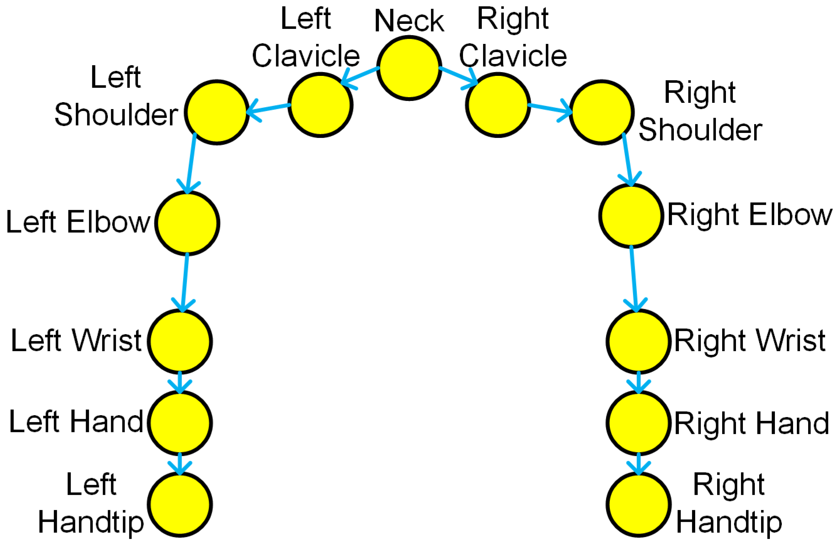
The human hands are the primary interaction objects for the robot during human–robot collaborative assembly process. To prevent collisions with human hands and upper body during robot motion, it is essential to predict the next future positions of the worker’s arms. Focusing on hand trajectory predicting during assembly process, this work considers the joints of a worker’s upper body, including neck, left (right) clavicle, left (right) shoulder, left (right) elbow, left (right) wrist, left (right) hand, and left (right) fingertip, representing a total of 13 joints which form a symmetrical structure. The human upper body skeleton is shown in Figure 1.

Figure 1.
Upper body skeleton.
The historical observation for frame length is represented as , where is the number of joints and represents the human pose at frame consisting of the 3D coordinates of joints, . The future human motion of length is . Given historical observation , human motion prediction aims to predict the future skeletal position sequence and to maximum the symmetry between and the ground truth .
3.2. Discrete Cosine Transform
The discrete cosine transform (DCT) transforms the joint coordinate trajectories from Cartesian space to trajectory space with a set of pre-constructed discrete orthogonal bases, and the original joint trajectories are then converted to linear combinations of the base trajectories. The DCT operation could extract both current and periodic temporal properties from the motion sequences, which more intuitively represents the motion dynamics of the joints and is beneficial for obtaining continuous motions [30]. In [18], the DCT operation was firstly applied to the motion prediction problem, and its effectiveness was verified. Therefore, keeping precedents [18], the DCT transform is firstly used to process the joint trajectory sequence.
Given an -frame motion sequence , the sequence is projected to the DCT domain via the DCT operation:
where is the predefined DCT basis and is the DCT coefficients. As the DCT transform is an orthogonal transform, the inverse discrete cosine transform iDCT can be used to recover the trajectory sequence based on the DCT coefficients. iDCT uses the transpose of as the basis matrix:
Considering the requirement of rapid response for HRC and the smoothness property of human motion, only the first rows of and are selected for the transformation denoted as , and an -frame trajectory is compressed into an -dimensional coefficient vector. Although this operation is a lossy compression of the original trajectory, it offers two benefits to MHP: (1) the high-frequency part of the motion dynamics is discarded, the subtle jitter of the prediction results will be reduced, and the predicted trajectory becomes smoother; and (2) by compressing the length of the sequence, computation costs during the training and inference are reduced, and the real-time performance is enhanced [18].
3.3. Fast Spatial–Temporal Transformer Network
The inter-joint spatial–temporal relationship in movement plays a vital role in human action prediction, and which were always modeled with RNNs or spatial–temporal GCNs. However, RNNs cannot understand the spatial structure well, and GCNs have limited temporal receptive field, which leads to their poor future prediction ability. On the full spatial–temporal resolution, Transformer models have stronger spatial–temporal perception and inference ability. However, due to the large number of linear layers, the model parameter number s is larger than RNNs or GCNs, which causes higher computing power requirements on HRC devices.
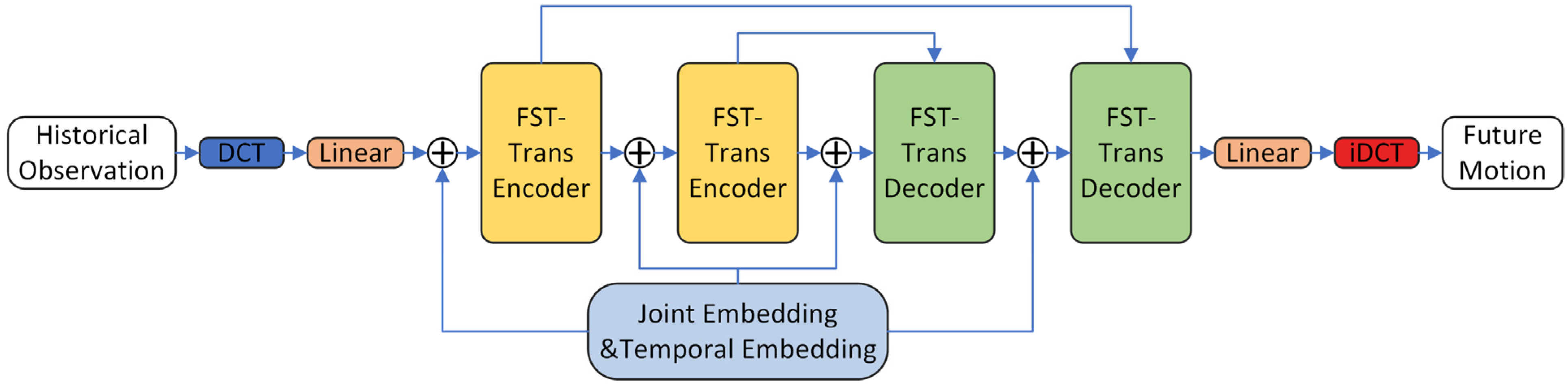
This work proposes the Fast Spatial–Temporal Transformer Network (FST-Trans) to address the above two issues. The FST-Transformer Network is designed with a symmetrical encoder–decoder structure, as shown in Figure 2:
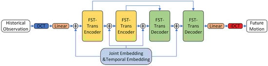
Figure 2.
Network structure.
Firstly, the historical observation is padded with its final frame to obtain an -frame sequence . After DCT transformation, the DCT coefficients are fed into the network. Feature embedding is performed by single linear layer, and the initial feature is obtained by adding the temporal position encoding and joints position encoding :
where , are both the learnable parameters, and represents the hidden dimension. The initial feature goes through layers of FST-Transformer block to obtain the final feature , using another single linear layer as the prediction head to get the DCT coefficients of the predicted trajectory:
Via an iDCT operation, a joint 3D coordinate trajectory can be obtained , and is the future motion estimation.
Both the encoder and decoder consist of FST-Trans blocks, and skip-layer connections are applied to minimize feature degeneracy. The sub-modules of single FST-Trans block include a temporal multi-head attention, a spatial multi-head attention, and a feed-forward neural network, and its computational flow is:
For the layer FST-Trans block, the input features are layer normalized by [31] firstly, and then the joint attention coefficients matrix and temporal attention coefficients matrix are computed, respectively, are all learnable weights for the feature vectors in the attention mechanism. and are computed via the multi-head attention method [24], and stands for operation:
After linear projection , the normalized feature is multiplied with the attention coefficient matrices and , and then added to the origin layer input feature to form the residual connection, and the layer normalization is performed to obtain the feature , which is used as the inputs for the feed-forward neural network (Equations (10) and (11)). In Equation (10), represents the GELU activation function [32], are two learnable weights, and are the learnable bias. The output of feed forward neural network is added to the layer input to obtain the block output feature .
The structure difference between FST-Trans block and 2-layer vanilla Transformer is demonstrated in Figure 3. To achieve spatial–temporal decoupled modeling [28,29], two Transformer blocks are usually necessary for single layer; spatial and temporal features are extracted in different latent spaces, respectively. Inspired by these results [33,34,35], this work tries to simplify and merge two vanilla Transformer Blocks for better feature extraction and computational efficiency. In FTS-Trans, the spatial attention mechanism shares vectors with the temporal attention. This design means the two attention coefficient matrices and act in the same latent space to fuse of the spatial–temporal features in a more compact manner. If the feature is reshaped into a 2D tensor , the application of the attention mechanism in the dimension can also achieve the simultaneous extraction of spatial–temporal features. Usually, the number of joints is pre-fixed, the size of attention coefficient matrix will be mainly influenced by the temporal dimension . To make longer-term predictions, the expanded temporal dimension will increase the runtime costs, affecting the real-time performance of HRC system. There are 10 learnable parameter matrices ( 2 each) in 2 Transformer blocks, and only 1 feed-forward neural network is kept in the FST-Trans block, so the number of learnable weights is reduced to 7. The number of layer normalization and activation functions are halved, which reduces the overall computational complexity significantly.
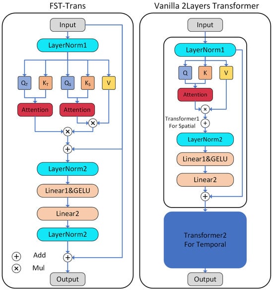
Figure 3.
FST-Trans block.
3.4. Loss Function
To train the proposed model, the reconstruction loss function is firstly defined as the average L2 distance between the real future joint motion and the predicted result, for one sample, which is calculated as follows:
where is joint’s prediction of 3D coordinates at frame, and is the corresponding ground truth.
Then, the spatial position of human pose is only one of the characteristics of human action, and the rate of movement and rate changes are also very distinctive human movement characteristics. When different individuals perform the same assembly process, the motion rate is often inconsistent due to various factors such as individual physical conditions and proficiency. To make the model learn the motion dynamic better, the velocity–acceleration loss was introduced, and the velocity of joint at the frame is:
and the acceleration is:
With the velocity–acceleration of real trajectory and predicted , the velocity–acceleration loss is:
where is the velocity–acceleration ground truth of the joint at the frame, and is the corresponding prediction value. The overall loss function is the sum of the reconstruction loss and the velocity–acceleration loss:
4. Experiment
Experiments are conducted on an assembly action dataset to evaluate the effectiveness of proposed model.
4.1. Dataset
The assembly dataset consists of 47 assembly videos with durations ranging from 10 to over 20 s. The following assembly actions are performed by nine different people: (1) taking and installing an interface; (2) taking the wrench to tighten the interface, and putting the wrench back in its original position after completion; (3) taking a bolt and installing it; (4) taking a nut and installing it; (5) taking the screwdriver to screw the bolt, and putting it back in its original position after completion. The videos were recorded using an Azure Kinect DK camera at 1080p@30FPS, and the 3D coordinates of the joints were extracted by the Kinect human body tracking SDK. A total of 40 videos were randomly selected as the training set, totaling 21,122 frames, while the remaining 7 videos were used for the test set, totaling 3123 frames. An example of data acquisition is shown in Figure 4.
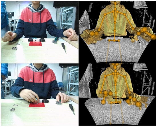
Figure 4.
Example of assembly dataset.
4.2. Metrics
Following previous works, two metrics are used as evaluation metrics: (1) Mean Per-Joint Position Error (MPJPE) is the average L2 distance between the predicted future joint position and the ground truth, computed in the same way as the loss function. (2) Final Displacement Error (FDE) is the L2 distance between the last frame of the prediction result and the corresponding ground truth. The lower the values of two indicators, the more accurate of the model prediction.
4.3. Implementation Details
The experimental model is composed of a four-layer FST-Trans Block with 256 hidden dimensions and eight attention heads. The model is trained on the training set for 300 Epochs with batch size of 64 by the Adam optimizer. The velocity–acceleration loss coefficient is set 0.1. The learning rate is initially 3 × 10⁻⁴, and a multistep learning rate decay strategy is adopted with a decay rate of 0.9. The dropout technique was applied on the attention coefficient matrix and the feed forward neural network to reduce overfitting with a dropout rate of 0.2. The object of this paper is long-term assembly motion prediction, so 25 frames (about 0.83 s) were selected as the historical motion, and 100 frames (about 3.3 s) were predicted, and the first 20 rows of the DCT matrix were taken for DCT operation. In terms of data processing, the results of the Kinect human body tracking SDK are in millimeters (mm) as the basic unit, and in order to prevent the gradient explosion caused by values that are too large, the original value is divided by 1000 to convert the unit to meters (m). The network model was implemented based on Pytorch [36] and trained on experimental platforms with 9700k CPU, 32GB RAM, and a single RTX4090 GPU.
4.4. Experiments Results
The comparison methods are a 12-layer GCN [18], skeletal-parted graph scattering network (SPGSN) [22], and spatial–temporal separatable graph convolutional network (STSGCN) [21], and the model settings follow the original work.
From Table 1, the lowest MPJPE (0.2473) and FDE (0.3011) values are both obtained by the proposed FST-Transformer Network, and the second lowest MPJPE (0.3288) and FDE (0.4083) values are obtained by the 12-layer GCN. The Transformer architecture models the overall spatial–temporal dynamics, and the motion feature extraction acts on the full spatial–temporal resolution, which results in a better overall motion perception capability. Comparison methods mostly use GCN for spatial modeling and TCN or T-GCN in temporal dimension where the receptive field only focuses on a local time period, resulting in insufficient long-term motion capture ability and then poor prediction results.

Table 1.
Experimental results of quantitative results.
The training time is the computational time consumption of one iteration of the train set with same batch size, the testing time is time consumption of whole test set. From Table 2, SPGSN has the largest number of parameters the highest training time and test inference time, while the parameters of STSGCN is smallest, and so is the time consumption. STSGCN’s low parameter number results in a lack of expression ability and poor prediction performance. Although the parameter number of the proposed FST-Trans is several times as that of STSGCN, the testing time and inference speed of FST-Trans are about the same as STSGCN with a higher prediction accuracy.
Table 2.
Parameters number and computation time costs.
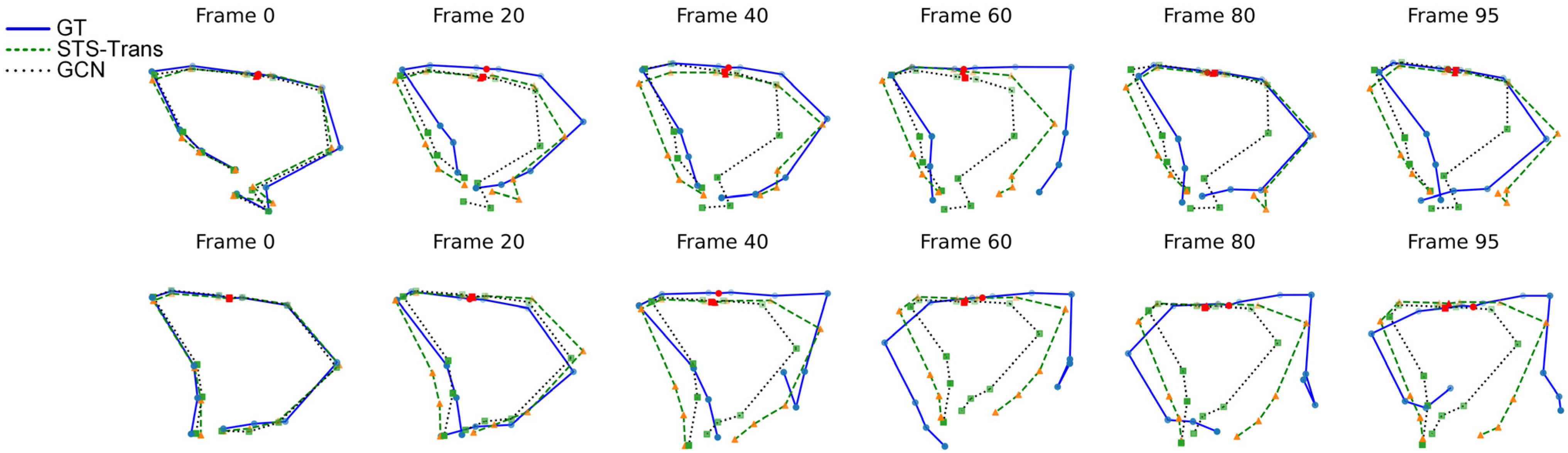
Figure 5 shows the visualization of the prediction results for the ground truth (blue straight line), FST-Trans (green dashed), and 12-layer GCN [18] (black dotted). It shows that the predicted poses of FST-Trans are closer to the ground truth than that of GCN, and the amplitude of the pose changes is also larger than that of GCN, which indicates that the proposed architecture has a stronger capability of modeling motion dynamics. However, when the prediction time span is large (after 60 frames), both results have a large deviation from the ground truth. In some cases, FTS-Trans can make predictions in line with the actual motion, but an accurate long-term prediction is still more difficult. The end hand position change is more difficult to capture, and how to predict the small range of subtle displacement better is a challenge in HMP. In summary, from both quantitative and qualitative result, it is clear that the proposed model outperformers than the comparison methods.
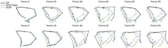
Figure 5.
Visualization results.
5. Ablation Discussion
For the proposed FST-Trans, ablation studies are discussed in five aspects, namely architecture design, hidden layer dimension , number of network layers , DCT coefficient dimension , and loss function, in order to verify the effectiveness of network design.
Comparison with vanilla Transformer. In this experiment, the 4-layer vanilla Transformer and FST-Trans’ hidden dimensions are both 256, and the number of layers is 4. In each layer of the comparison model, there are two Transformer blocks, respectively, for extracting features in joint and temporal dimensions, resulting in a total of eight original Transformer Blocks. From Table 3, The FST-Trans achieved a better prediction accuracy with fewer parameters, which indicates that the structural design of FST-Trans is more concise and effective.
Table 3.
Four-layer vanilla Transformer vs. FST-Trans.
Hidden Dimension. In Table 4, when is 512, the minimal FDE is 0.2905; and the MPJPE is smallest when is 256. Usually, an increase in the hidden dimension will increase the network characterization ability. In the experimental environment of this work, the performance is not significantly improved when the hidden layer dimension increases; instead, it works best when . Therefore, considering the dataset size and computational complexity, 256 is chosen as the optimal hidden dimension.
Table 4.
Hidden dimension.
The number of network layers. From Table 5, when the number of network layers is 2, both MPJPE and FDE are at their maximum, and the prediction performance is the worst; the min-MPJPE value is in the 4-layer network, and the min-FDE value is in the 6-layer network. The prediction performance does not increase significantly with the increase in the network layers, and the characterization ability of the 4-layer FST-Trans network with 256 hidden dimensions can satisfy the requirement.
Table 5.
The number of network layers.
DCT coefficients dimension. In Table 6, when the first 25 rows of the DCT matrix are taken for transformation, the MPJPE rises to 0.2555 and the FDE rises to 0.3057; when the first 15 rows of the DCT matrix are taken, the MPJPE rises to 0.2577 and the FDE rises to 0.3130. The best result is achieved when , and any change in the DCT domain coefficients can negatively affect the motion prediction.
Table 6.
DCT coefficients dimension.
In Table 7, without DCT, the network takes 125-frame trajectory sequences (25 frames of history and 100 frames of padding) as the input. Due to the expansion of the temporal dimension by a factor of 6.25, the training time goes up by a factor of 6.95 consequently, and the MPJPE goes up by a factor of 0.0147, and the bias of prediction results increases. Therefore, the use of DCT not only reduces the computation costs, but also helps to improve the prediction accuracy.
Table 7.
Ablation w/ or w/o DCT transform.
The effect of the velocity–acceleration loss coefficient α on the prediction performance is demonstrated in Table 8. When , the min-MPJPE value is 0.2473 and the min-FDE value is 0.3011. Increasing α to 0.2, the model shows a slight performance degradation. α = 0 represents the non-use of velocity–acceleration loss. Comparing with , the MPJPE of α = 0 rises by 0.01, while the FDE decreases by 0.0081. The introduction of the velocity–acceleration loss has a positive impact on the prediction performance. Considering that the MPJPE reflects the overall similarity of the trajectories, it is more appropriate to take to be 0.1.
Table 8.
Vel–acc loss coefficient.
6. Conclusions and Discussion
In this work, a network model for predicting hand motion in human–robot collaborative assembly is introduced. The model utilizes the FST-Trans block, a simplified version of vanilla Transformer, to extract spatial–temporal features in a unified latent space. Additionally, the introduction of velocity–acceleration loss improves the model’s ability to learn temporal dynamic, finally achieving rapid and accurate motion prediction for human–robot collaborative assembly. As can be seen from the evaluation metrics and visualization of the results, the 4-layer FST-Trans network with a hidden dimension of 256 and DCT coefficient achieves the optimal results with an MPJPE of 0.2473 on the assembly dataset, which is better than the second lowest MPJPE of 0.3288 via the 12-layer GCN [18]. Compared with the vanilla Transformer, not only do the parameters of the proposed model decrease by about 12.5%, but also the prediction accuracy improves. The testing time of the proposed model is only slightly larger than of STSGCN [21], which has the least number of parameters. Other ablation experiments’ results have shown that the method performance decreases when DCT and velocity–acceleration loss are removed, and thus, the initial hypothesis has been verified.
Although the effectiveness of the network design has been verified, as shown in the visualization of results, there is significant deviation in hand position especially when the prediction time is long. Accurately depicting tiny hand displacements remains a challenge. As hand movements are mainly involved in the assembly process, the movements of the shoulders and other joints are less significant. Therefore, the motion prediction model should pay more attention to hands, and improving the weight of hand movements could be a promising direction. A larger dataset size may bring a performance gain, and the size of the assembly dataset will be expanded in the future. And the combination of motion prediction and robot path planning will also be a future research focus. Reinforcement learning, a method of learning decision-making strategies in response to changes in the environment, is commonly used to enhance collaboration between humans and robots [37,38,39,40,41]. Accurate motion prediction is for better human–robot collaboration, and the feedback of HRC maybe also helpful to HMP. Reinforcement learning could act as a bridge between HMP and HRC.
Author Contributions
Conceptualization, Y.Z., P.L. and L.L.; methodology, Y.Z.; software, Y.Z.; validation, P.L. and L.L.; formal analysis, Y.Z.; investigation, Y.Z. and L.L.; resources, P.L. and L.L.; data curation, Y.Z.; writing—original draft preparation, Y.Z.; writing—review and editing, P.L. and L.L.; visualization, Y.Z.; supervision, P.L.; project administration, P.L.; funding acquisition, P.L. All authors have read and agreed to the published version of the manuscript.
Funding
This work was supported by the Fundamental Research Funds for the Central Universities (22120220666).
Data Availability Statement
The datasets presented in this article are not readily available because the data are part of an ongoing study. Requests to access the datasets should be directed to the authors.
Acknowledgments
The authors are grateful to the other graduate and doctoral students of our team for their equipment support and data capture assistance.
Conflicts of Interest
The authors declare no conflicts of interest.
References
- Weiss, A.; Wortmeier, A.K.; Kubicek, B. Cobots in industry 4.0: A roadmap for future practice studies on human–robot collaboration. IEEE Trans. Hum. Mach. Syst. 2021, 51, 335–345. [Google Scholar] [CrossRef]
- Bragança, S.; Costa, E.; Castellucci, I.; Arezes, P.M. A brief overview of the use of collaborative robots in industry 4.0: Human role and safety. Occup. Environ. Saf. Health 2019, 202, 641–650. [Google Scholar]
- Goel, R.; Gupta, P. Robotics and industry 4.0. A Roadmap to Industry 4.0: Smart Production. In Sharp Business and Sustainable Development; Springer: Berlin/Heidelberg, Germany, 2020; pp. 157–169. [Google Scholar]
- Lea, C.; Vidal, R.; Reiter, A.; Hager, G.D. Temporal convolutional networks: A unified approach to action segmentation. In Proceedings of the Computer Vision–ECCV 2016 Workshops, Amsterdam, The Netherlands, 8–10 October 2016; Part III 14. pp. 47–54. [Google Scholar]
- Choi, A.; Jawed, M.K.; Joo, J. Preemptive motion planning for human-to-robot indirect placement handovers. In Proceedings of the 2022 International Conference on Robotics and Automation, Philadelphia, PA, USA, 23–27 May 2022; pp. 4743–4749. [Google Scholar]
- Unhelkar, V.V.; Lasota, P.A.; Tyroller, Q.; Buhai, R.D.; Marceau, L.; Deml, B.; Shah, J.A. Human-aware robotic assistant for collaborative assembly: Integrating human motion prediction with planning in time. IEEE Robot. Autom. Lett. 2018, 3, 2394–2401. [Google Scholar] [CrossRef]
- Khawaja, F.I.; Kanazawa, A.; Kinugawa, J.; Kosuge, K. A Human-Following Motion Planning and Control Scheme for Collaborative Robots Based on Human Motion Prediction. Sensors 2021, 21, 8229. [Google Scholar] [CrossRef] [PubMed]
- Vianello, L.; Mouret, J.B.; Dalin, E.; Aubry, A.; Ivaldi, S. Human posture prediction during physical human-robot interaction. IEEE Robot. Autom. Lett. 2021, 6, 6046–6053. [Google Scholar] [CrossRef]
- Cheng, Y.; Zhao, W.; Liu, C.; Tomizuka, M. Human motion prediction using semi-adaptable neural networks. In Proceedings of the 2019 American Control Conference, Philadelphia, PA, USA, 10–12 July 2019; pp. 4884–4890. [Google Scholar]
- Cheng, Y.; Sun, L.; Liu, C.; Tomizuka, M. Towards efficient human-robot collaboration with robust plan recognition and trajectory prediction. IEEE Robot. Autom. Lett. 2020, 5, 2602–2609. [Google Scholar] [CrossRef]
- Fragkiadaki, K.; Levine, S.; Felsen, P.; Malik, J. Recurrent network models for human dynamics. In Proceedings of the 2015 IEEE International Conference on Computer Vision, Santiago, Chile, 7–13 December 2015; pp. 4346–4435. [Google Scholar]
- Kratzer, P.; Midlagajni, N.B.; Toussaint, M.; Mainprice, J. Anticipating human intention for full-body motion prediction in object grasping and placing tasks. In Proceedings of the 29th IEEE International Conference on Robot and Human Interactive Communication (RO-MAN), Naples, Italy, 31 August–4 September 2020; pp. 1157–1163. [Google Scholar]
- Zhang, J.; Liu, H.; Chang, Q.; Wang, L.; Gao, R.X. Recurrent neural network for motion trajectory prediction in human-robot collaborative assembly. CIRP Ann. 2020, 69, 9–12. [Google Scholar] [CrossRef]
- Ivanovic, B.; Leung, K.; Schmerling, E.; Pavone, M. Multimodal deep generative models for trajectory prediction: A conditional variational autoencoder approach. IEEE Robot. Autom. Lett. 2020, 6, 295–302. [Google Scholar] [CrossRef]
- Lyu, J.; Ruppel, P.; Hendrich, N.; Li, S.; Görner, M.; Zhang, J. Efficient and collision-free human-robot collaboration based on intention and trajectory prediction. IEEE Trans. Cogn. Dev. Syst. 2023, 15, 1853–1863. [Google Scholar] [CrossRef]
- Kipf, T.N.; Welling, M. Semi-supervised classification with graph convolutional networks. arXiv 2016, arXiv:1609.02907. [Google Scholar]
- Yan, S.; Xiong, Y.; Lin, D. Spatial temporal graph convolutional networks for skeleton-based action recognition. In Proceedings of the AAAI Conference on Artificial Intelligence, New Orleans, LA, USA, 27 April 2018; Volume 32. [Google Scholar]
- Mao, W.; Liu, M.; Salzmann, M.; Li, H. Learning trajectory dependencies for human motion prediction. In Proceedings of the IEEE/CVF International Conference on Computer Vision, Seoul, Republic of Korea, 27 October–2 November 2019; pp. 9489–9497. [Google Scholar]
- Cui, Q.; Sun, H.; Yang, F. Learning dynamic relationships for 3d human motion prediction. In Proceedings of the 2020 IEEE/CVF Conference on Computer Vision and Pattern Recognition, Seattle, WA, USA, 19 June 2020; pp. 6518–6526. [Google Scholar]
- Dang, L.; Nie, Y.; Long, C.; Zhang, Q.; Li, G. Msr-gcn: Multi-scale residual graph convolution networks for human motion prediction. In Proceedings of the IEEE/CVF International Conference on Computer Vision, Montreal, QC, Canada, 10–17 October 2021; pp. 11467–11476. [Google Scholar]
- Sofianos, T.; Sampieri, A.; Franco, L.; Galasso, F. Space-time-separable graph convolutional network for pose forecasting. In Proceedings of the IEEE/CVF International Conference on Computer Vision, Montreal, QC, Canada, 10–17 October 2021; pp. 11209–11218. [Google Scholar]
- Li, M.; Chen, S.; Zhang, Z.; Xie, L.; Tian, Q.; Zhang, Y. Skeleton-parted graph scattering networks for 3d human motion prediction. In Proceedings of the European Conference on Computer Vision, Tel Aviv, Israel, 23–27 October 2022; pp. 18–36. [Google Scholar]
- Sampieri, A.; di Melendugno, G.M.D.A.; Avogaro, A.; Cunico, F.; Setti, F.; Skenderi, G.; Cristani, M.; Galasso, F. Pose forecasting in industrial human-robot collaboration. In Proceedings of the European Conference on Computer Vision, Tel Aviv, Israel, 23–27 October 2022; pp. 51–69. [Google Scholar]
- Vaswani, A.; Shazeer, N.; Parmar, N.; Uszkoreit, J.; Jones, L.; Gomez, A.N.; Kaiser, Ł.; Polosukhin, I. Attention is all you need. In Proceedings of the 31st International Conference on Neural Information Processing Systems, Long Beach, CA, USA, 4–9 December 2017; pp. 6000–6010. [Google Scholar]
- Lucas, T.; Baradel, F.; Weinzaepfel, P.; Rogez, G. Posegpt: Quantization-based 3d human motion generation and forecasting. In Proceedings of the European Conference on Computer Vision, Tel Aviv, Israel, 23–27 October 2022; pp. 417–435. [Google Scholar]
- Mao, W.; Liu, M.; Salzmann, M. Weakly-supervised action transition learning for stochastic human motion prediction. In Proceedings of the IEEE/CVF Conference on Computer Vision and Pattern Recognition, New Orleans, LA, USA, 18–24 June 2022; pp. 8151–8160. [Google Scholar]
- Tevet, G.; Raab, S.; Gordon, B.; Shafir, Y.; Cohen-Or, D.; Bermano, A.H. Human motion diffusion model. arXiv 2022, arXiv:2209.14916. [Google Scholar]
- Zhu, W.; Ma, X.; Liu, Z.; Liu, L.; Wu, W.; Wang, Y. Motionbert: A unified perspective on learning human motion representations. In Proceedings of the IEEE/CVF International Conference on Computer Vision, Paris, France, 1–6 October 2023; pp. 15085–15099. [Google Scholar]
- Yu, C.; Ma, X.; Ren, J.; Zhao, H.; Yi, S. Spatio-temporal graph transformer networks for pedestrian trajectory prediction. In Proceedings of the European Conference on Computer Vision, Glasgow, UK, 23–28 August 2020; Part XII 16. pp. 507–523. [Google Scholar]
- Akhter, I.; Sheikh, Y.; Khan, S.; Kanade, T. Nonrigid structure from motion in trajectory space. In Proceedings of the 21st International Conference on Neural Information Processing Systems, Vancouver, BC, Canada, 8–10 December 2008; pp. 41–48. [Google Scholar]
- Ba, J.L.; Kiros, J.R.; Hinton, G.E. Layer normalization. arXiv 2016, arXiv:1607.06450. [Google Scholar]
- Hendrycks, D.; Gimpel, K. Gaussian error linear units (gelus). arXiv 2016, arXiv:1606.08415. [Google Scholar]
- Hayou, S.; Clerico, E.; He, B.; Deligiannidis, G.; Doucet, A.; Rousseau, J. Stable resnet. In Proceedings of the International Conference on Artificial Intelligence and Statistics, Virtual, 13–15 April 2021; pp. 1324–1332. [Google Scholar]
- He, B.; Martens, J.; Zhang, G.; Botev, A.; Brock, A.; Smith, S.L.; Teh, Y.W. Deep Transformers without Shortcuts: Modifying Self-attention for Faithful Signal Propagation. In Proceedings of the Eleventh International Conference on Learning Representations, Virtual, 25–29 April 2022. [Google Scholar]
- He, B.; Hofmann, T. Simplifying Transformer Blocks. arXiv 2023, arXiv:2311.01906. [Google Scholar]
- Paszke, A.; Gross, S.; Massa, F.; Lerer, A.; Bradbury, J.; Chanan, G.; Killeen, T.; Lin, Z.; Gimelshein, N.; Antiga, L.; et al. Pytorch: An imperative style, high-performance deep learning library. In Proceedings of the 33rd International Conference on Neural Information Processing Systems, Vancouver, BC, Canada, 8–14 December 2019; pp. 8026–8037. [Google Scholar]
- Mohammed, W.M.; Nejman, M.; Castaño, F.; Lastra, J.L.M.; Strzelczak, S.; Villalonga, A. Training an Under-actuated Gripper for Grasping Shallow Objects Using Reinforcement Learning. In Proceedings of the 2020 IEEE Conference on Industrial Cyberphysical Systems (ICPS), Tampere, Finland, 10–12 June 2020; Volume 1, pp. 493–498. [Google Scholar]
- Goel, P.; Mehta, S.; Kumar, R.; Castaño, F. Sustainable Green Human Resource management practices in educational institutions: An interpretive structural modelling and analytic hierarchy process approach. Sustainability 2022, 14, 12853. [Google Scholar] [CrossRef]
- Zhang, R.; Lv, Q.; Li, J.; Bao, J.; Liu, T.; Liu, S. A reinforcement learning method for human-robot collaboration in assembly tasks. Robot. Comput. Integr. Manuf. 2022, 73, 102227. [Google Scholar] [CrossRef]
- Oliff, H.; Liu, Y.; Kumar, M.; Williams, M.; Ryan, M. Reinforcement learning for facilitating human-robot-interaction in manufacturing. J. Manuf. Syst. 2020, 56, 326–340. [Google Scholar] [CrossRef]
- El-Shamouty, M.; Wu, X.; Yang, S.; Albus, M.; Huber, M.F. Towards safe human-robot collaboration using deep reinforcement learning. In Proceedings of the 2020 IEEE international conference on robotics and automation (ICRA), Paris, France, 31 May–31 August 2020; pp. 4899–4905. [Google Scholar]


Disclaimer/Publisher’s Note: The statements, opinions and data contained in all publications are solely those of the individual author(s) and contributor(s) and not of MDPI and/or the editor(s). MDPI and/or the editor(s) disclaim responsibility for any injury to people or property resulting from any ideas, methods, instructions or products referred to in the content. |
© 2024 by the authors. Licensee MDPI, Basel, Switzerland. This article is an open access article distributed under the terms and conditions of the Creative Commons Attribution (CC BY) license (https://creativecommons.org/licenses/by/4.0/).